Probing large distance higher dimensional gravity from lensing data.

Abstract

The modifications induced in the standard weak-lensing formula if Newtonian gravity differs from inverse square law at large distances are studied. The possibility of putting bounds on the mass of gravitons from lensing data is explored. A bound on graviton mass, esitmated to be about 100 Mpc^-1 is obtained from analysis of some recent data on gravitational lensing.

Ever since the successful unification of weak and e.m. interactions into an ‘electroweak’ theory, hopes have been raised for extensions of these ideas to strong interactions ( Grand Unified Theories) and even further to a full unified theory including Gravitation as well. One of the foremost difficulties in incorporating gravity with the electroweak theory concerns the so called ‘hierarchy’ problem namely the huge difference in the scales of the electroweak theory which is $\sim$ 1 TeV, with that of quantum gravity which is much higher at $10^{19}$ GeV. During the last four years, an attractive idea has been introduced [1] to overcome the hierarchy problem based on a higher dimensional space time scenario. In the earliest of such approaches, space-time is (4+n) dimensional with the n-extra spatial dimensions compact. Matter through Standard Model (SM) - fields is proposed to be confined to the 4-dimensional slice while gravity being the metric field is all over. There is only one basic Planck scale in the theory comparable to the TeV-scale electroweak scale. The weakness of gravitational interactions in our 4-dimensional world comes about through the celebrated relation:

$$M_{Pl,4-\mbox{{\scriptsize dim}}}^{2}=M_{Pl,(4+n)-\mbox{{\scriptsize dim}}}^{2+n}R^{n}$$ (1)

where R is the size of the compact dimensions. The law of gravity remains practically unchanged with a 4-dimensional Planck scale for distances $r>>R$ whereas for $r<<R$ the gravitational law changes to a $\frac{1}{r^{1+n}}$ potential with a scale determined by $M_{Pl}^{4+n}$. Thus, as far as the validity of Newton’s law is concerned, deviations can be explored in the small distance region, lower than the current experimental limits.[9] 

Subseqently, Randall and Sundrum(RS) [2] proposed a somewhat different higher dimensional scenario which once again solves the hierarchy problem. The RS construction is in a total of 5-dimensions, with the fifth dimension in the form of a compact torus with opposite points identified. At the fixed points of the $S^{1}/Z_{2}$ orbifold, one has two 3-branes wherein the SM fields are confined at one end and a ’hidden’ world is confined in the other. It is further assumed that there is a negative tension in our brane and a positive tension in the other and also a bulk cosmological constant. With the tensions in the brane and bulk finely tuned , one can solve the 5- dimensional Einstein equations to get a non- factorizable metric with an exponential ‘warp’ factor. The five dimensional Planck scale in this model is comparable to our Planck scale but the ‘warp’ factor effectively reduces all mass scales in our theory including the vev of the scalar field in the electroweak theory to the TeV range. The hierarchy problem is thus solved indirectly. Once again in this theory there are no deviations of the gravitation law at large distance. 

The RS scenario above is in a matter free universe. In the presence of matter, complications arise in the form of the theory not being able to reproduce standard cosmological results like the dependence of the Hubble constant on the matter density. This arises essentially because, in this model, we live in the negative tension brane. It is in this context, that extensions of the RS scenario have been proposed [4] wherein there are more branes and we live in a positive tension brane. The most notable feature of these extensions is the possibility of deviations from Newtonian gravity at large distances. Thus , in the model of Kogan et.al., in addition to a massless graviton one also has a massive graviton with a tiny mass which is coupled strongly relative to the massless one. The effective Planck scale that we see, $M_{Pl}$, gets related to the Planck scale of the theory, $M$, by the relation:

$$\frac{1}{M_{Pl}^{2}}=\frac{1}{M^{2}}.\big{[}1+\frac{1}{w^{2}}\big{]}$$ (2)

where $w$ is the ’warp’ factor typical of the RS kind of scenario. Since $w$ is a small number compared to unity, gravity is essentially dominated by the graviton with a tiny mass rather than by the massless one. This would imply that at large distances gravity will fall like an Yukawa potential rather than a pure 1/r law. The theory is unable to give any estimate of the mass of this graviton. Laboratory experiments to put bounds on this of course are useless since we know that Newtonian gravity works very well at least upto planetary scales. One thus has to look into possible cosmological measurables to detect possible violations of Newtonian gravity law. 

In a number of other models which have a modification of gravity at large distances [5], the transition can be modelled as a Yukawa modification of the Newtonian potential, and can be analysed as if one has a finite graviton mass.

It is in the context of the motivation outlined above that we address the question of the sensitivity of gravitational lensing measurements to possible deviations from Newtonian gravity. Admittedly, cosmological theories do not have the same theoretical precision of theories like the SM but it will still be useful to know the nature of deviations from Newtonian gravity that current precision of gravitational lensing data can accomodate.  

In this note we focus our attention to a very recent measurement of gravitational lensing parameters by a cluster of stars at around an average redshift of $z=1.2$ [3] to evaluate the compatibility of the data with a ‘massive’ graviton. We follow the standard treatment of the relationship between the ‘lensing’ parameters and density fluctuations [6]. In the standard gravitational scenario, the power spectrum $P_{\kappa}(l)$ of the effective convergence is given by, assuming a flat universe:[6]

$$P_{\kappa}(l) = \frac{9H_{0}^{4}\Omega_{m}^{2}}{4c^{4}}\int_{0}^{w_{H}}dw\frac{W^{2}(w)}{a^{2}(w)}P_{\delta}(\frac{l}{w},w)$$ (3)

In the last equation, $\Omega_{m}$ is the matter density scaled to the critical density, $w_{H}$ is the horizon distance, $a(w)$ is the scale factor related to the redshift by the relation $a^{-1}=(1+z)$, $W(w)$ is related to the normalized source distribution function G(w) by

$$W(w)=\int_{w}^{w_{H}}dw^{\prime}G(w^{\prime})\big{(}1-\frac{w}{w^{\prime}}\big{)}$$ (4)

and $P_{\delta}(k,w)$ is the density contrast function at a distance $w$. For a single source at $w=w_{s}$ , we have

$$G(w)=\delta(w-w_{s})$$

and $P_{\kappa}$ reduces to

$$P_{\kappa}=\frac{9H_{0}^{4}\Omega_{m}^{2}}{4c^{4}}\int_{0}^{w_{s}}dw\big{(}1-\frac{w}{w_{s}}\big{)}^{2}\frac{1}{a^{2}(w)}P_{\delta}(\frac{l}{w},w)$$ (5)

The modification of this last equation, if the graviton has a mass m is easily obtained by observing that the density contrast function enters the rhs of the equation through the relation between the gravitational potential $\Phi$ and the density fluctation $\delta$:

$$\nabla^{2}\Phi=\frac{3H_{0}^{2}\Omega_{m}^{2}}{2a}\delta$$ (6)

which becomes a simple multiplicative relation in Fourier space. This last equation gets modified, if the gravitation field has the Yukawa form $\frac{e^{-\mu r}}{r}$ instead of a pure 1/r form, into

$$\big{(}\nabla^{2}-m^{2}\big{)}\Phi=\frac{3H_{0}^{2}\Omega_{m}^{2}}{2a}\delta$$ (7)

so that the power spectrum $P_{\kappa}(l)$ gets modified t $P_{\kappa}^{m}(l)$ given by

$$P_{\kappa}^{m}(l)=\frac{9H_{0}^{4}\Omega^{2}}{4c^{4}}\int_{0}^{w_{s}}dw\frac{P_{\delta}(\frac{l}{w},w)}{a^{2}(w)}\Big{[}\frac{\frac{l^{2}}{w^{2}}}{\frac{l^{2}}{w^{2}}+m^{2}}\Big{]}^{2}$$ (8)

The equations for $P_{\kappa}$ and $P_{\kappa}^{m}$ are the two basic results that we shall use to compute the effect of massive gravitons. For this purpose, we focus our attention on a recent extensive measurement of lensing data from a cluster at around an average redshift of z=1.2. In particular we shall concentrate on the measured values of the variance of the power spectrum $\gamma^{2}$ smoothed over a filter of radius $\theta$ which is related to the $P_{\kappa}$ by:

$$\gamma^{2}(\theta)=\frac{2}{\pi\theta^{2}}\int_{0}^{\infty}dlP_{\kappa}(l)J_{1}^{2}(l\theta),$$ (9)

where for simplicity we ignore the variation of the redshifts of the sources and assume that the entire cluster is at z=1.2. For the density contrast spectrum $P_{\delta}$, we assume a form:

$$P_{\delta}(k,w) = N.kT_{k}^{2}(q)a^{2}(w)$$

$$q = \frac{k}{\Omega h^{2}},$$ (10)

where N is the normalization constant and $T_{k}(q)$ is given by [8]

$$T_{k}(q)=\frac{log(1+2.34q)}{2.34q}[1+3.89q+(16.1q)^{2}+(5.46q)^{3}+(6.71q)^{4}]^{-\frac{1}{4}}$$ (11)

N is determined as usual by a $\sigma_{8}$ normalization procedure so that it is determined with the value of $\sigma_{8}$ as a parameter. To account for the non-linear evolution, we do not use the expression for $P_{\delta}(k,w)$ as above directly but use it to determine the expression for the density power spectrum evolved according to the HKLM procedure.[8] This involves defining an integration variable $k_{nl}$ in the integrals above and a non-linear power-spectrum $\Delta^{2}_{nl}(k_{nl})$ as follows:[8]

$$\Delta^{2}_{l}(k_{l},w) = \frac{k_{l}^{3}}{2\pi^{2}}P_{\delta}(k,w)$$

$$\Delta^{2}_{nl}(k_{nl},w) = f_{nl}(\Delta^{2}_{l}(k_{l},w))$$

$$f_{nl}(x) = x\big{[}\frac{1+N(x)}{1+D(x)}\big{]}^{\frac{1}{\beta}}$$

$$N(x) = B\beta x+\big{(}Ax\big{)}^{\alpha\beta}$$

$$D(x) = \Big{[}\frac{(Ax)^{\alpha}g^{3}(\Omega)}{V\sqrt{(}x)}\Big{]}^{\beta}.$$ (12)

The constants A, B, V, $\alpha$, $\beta$ and g are defined as follows:[10]

$$A = 0.482(1+n/3)^{-0.947}$$

$$B = 0.226(1+n/3)^{-1.778}$$

$$\alpha = 3.310(1+n/3)^{-0.344}$$

$$\beta = 0.862(1+n/3)^{-0.287}$$

$$V = 11.55(1+n/3)^{-0.423}$$

$$g = \frac{5}{2}\Omega_{m}\big{[}\Omega_{m}^{\frac{4}{7}}-\Omega_{v}+(1+\frac{1}{2}\Omega_{m})(1+\frac{\Omega_{v}}{70})\big{]}^{-1}.$$ (13)

$\Omega$ in the above equations is the sum of the matter density $\Omega_{m}$ and the vacuum contribution $\Omega_{v}$. Finally the spectral index n used above is determined as a function of k via the equation

$$n=\frac{dlog(P_{\delta(k)})}{dlog(k)}.$$ (14)

The numerical calculation above thus involves four parameters, $\sigma_{8}$, h, and $\Omega_{m}$ assuming a flat universe and also assuming the form of the Dark matter spectrum given above. At first it seems hopeless to obtain any useful information for the mass m but it is not actually so. Looking at the graph of the measured variable $\gamma^{2}$ versus the angle $\theta$ as shown in Fig.1, it is clear that at low angles the value of $\gamma^{2}$ is not affected by the presence of the mass or otherwise. In other words, we can use the value of $\gamma^{2}$ in effect to fix our parameters. With the parameters fixed thus, we can estimate the values of the same quantity $\gamma^{2}$ at larger angles which now is sensitive to the presence or otherwise of a graviton mass. 

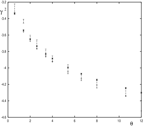
Figure 1: Our fit to the variance data referred to in the text for values of h=0.21, $\sigma_{8}$=0.85 and $\Omega_{m}$= 0.3. The points marked * refer to the usual Newtonian gravity whereas the points marked + uses a modified Newtonian law with a mass m chosen to be $m^{-1}$=100 Mpc; this value is chosen so that the spread of the points at the higher angle values along the x-axis approximately equals the error bars.

Figure 1 summarizes our result for the best fit obtained with values of h=0.21, $\sigma_{8}$=0.85 and $\Omega_{m}=0.3$ in the context of our flat universe model. Using these, we see that at higher values of the angle, the precision of the experimental values is compatible with mass m such that

$$m^{-1}=100Mpc$$ (15)

or higher i.e. masses heavier than about the inverse of 100 Mpc seem to be ruled out. A similar limit has been found in an analysis of planetry orbits by Gruzinov [11]. It has been estimated by Binetruy and Silk [7] that current precision of Cosmic microwave background gives some kind of a limit once again on the effective graviton mass, which according to their estimate is

$$m^{-1}\geq r_{h,ls}$$ (16)

where $r_{h,ls}$ is the horizon distance at last scattering, which is of order 3 Mpc for a Hubble Constant of 75 Km s^-1 Mpc^-1. Our estimate, although less direct, provides a better limit to this quantity. 

In conclusion, gravitational lensing data provides a window for the detection of deviations from Newtonian gravity at large distances . A present crude estimate is deviations if at all can occur at distances beyond 100 Mpc. With more refined data and some more definitive estimates of various cosmological parameters, this can certainly be improved.

References

- [1] N. Arkani-Hamed, S. Dimopoulos and G. R. Dvali, Phys. Lett. B 429, 263 (1998) [arXiv:hep-ph/9803315]; N. Arkani-Hamed, S. Dimopoulos and G. R. Dvali, Phys. Rev. D 59, 086004 (1999) [arXiv:hep-ph/9807344]; I. Antoniadis, N. Arkani-Hamed, S. Dimopoulos and G. R. Dvali, Phys. Lett. B 436, 257 (1998) [arXiv:hep-ph/9804398].
- [2] L. Randall and R. Sundrum, Phys. Rev. Lett. 83, 3370 (1999) [arXiv:hep-ph/9905221].
- [3] L. V. Waerbeke et al., arXiv:astro-ph/0101511.
- [4] I. I. Kogan, S. Mouslopoulos, A. Papazoglou and G. G. Ross, Nucl. Phys. B 595, 225 (2001) [arXiv:hep-th/0006030].
- [5] See for example G. R. Dvali, G. Gabadadze, M. Kolanovic and F. Nitti, Phys. Rev. D 65, 024031 (2002) [arXiv:hep-th/0106058]; G. R. Dvali, G. Gabadadze, M. Kolanovic and F. Nitti, Phys. Rev. D 64, 084004 (2001) [arXiv:hep-ph/0102216]; G. R. Dvali, G. Gabadadze and M. Porrati, Phys. Lett. B 485, 208 (2000) [arXiv:hep-th/0005016].
- [6] M. Bartelmann and P. Schneider, Physics Reports 340,291(2001) (1999); P. Schneider et.al., MNRAS,296,873 (1998).
- [7] P. Binetruy and J. Silk, Phys. Rev. Lett. 87, 031102 (2001) [arXiv:astro-ph/0007452].
- [8] J. A. Peacock, “Cosmological Physics,” Cambridge, UK: Univ. Pr. (1999) 682 p.
- [9] C. D. Hoyle, U. Schmidt, B. R. Heckel, E. G. Adelberger, J. H. Gundlach, D. J. Kapner and H. E. Swanson, Phys. Rev. Lett. 86, 1418 (2001) [arXiv:hep-ph/0011014].
- [10] J. A. Peacock and S. J. Dodds , MNRAS 280 ,L19 (1996)
- [11] A. Gruzinov, arXiv:astro-ph/0112246.