Recent experimental data and the size of
 
the quark in the Constituent Quark Model

Abstract

We use the Constituent Quark Model (CQM) to describe CDF data on double parton cross section and HERA data on the $\,J\,/\,\Psi$ ratio cross section of elastic and inelastic diffractive productions. Our estimate shows that the radius of the constituent quark turns out to be rather small, $R^{2}_{quark}\,\approx\,0.1\,Gev^{-2}$, in accordance with the assumption on which CQM is based.

TAUP - 2700-2002

1 Introduction

One of the most challenging problems of QCD is to find correct degrees of freedom for high energy “soft” interaction. In other words, the question is what set of quantum numbers diagonalizes the interaction matrix at high energies. On the one hand, the observation of the diffraction production in all “soft” processes including the photoproduction [1] is a direct experimental indication that hadrons are not correct degrees of freedom. On the other hand, at short distances we know that colour dipoles are the correct degrees of freedom [2] (see also Refs. [3] ). Frankly speaking, these two facts exhaust our solid theoretical knowledge on the subject.

In this paper we are going to examine an old model for the degrees of freedom at high energy: the Constituent Quark Model[4], in which the constituent quarks play the rôle of the correct degrees of freedom. In spite of the naivity of this model it works and describes a lot of “soft” data in the first approximation [5].

Different theoretical arguments have also been expressed in favour of the existence of two sizes in hadrons, e.g. in instanton models of QCD vacuum [6] and it has been included as an essential ingredient in the non-perturbative QCD approach for the high energy scattering [7]. The CQM gives a constructive way to build an approach which introduces two dimensional scales inside a hadron: the size of the hadron, built of the constituent quarks and the size of the constituent quark itself.

We wish to re-examine this model because of two beautiful pieces of the experimental data.

1. CDF double parton cross section at the Tevatron [8]. The CDF collaboration has measured the process of inclusive production of two pairs of “hard” jets with almost compensating transverse momenta in each pair, and with values of rapidity that are very similar. Such pairs can only be produced in double parton shower interactions (double parton collisions, see Fig. 1). The cross section of this interaction can be calculated using Mueller diagrams (as shown in Fig. 1) in CQM.

Figure 1: The Mueller diagram for the double parton shower interaction.

The double parton scattering cross section can be written in the form [8]

$$\sigma_{DP}\,\,=\,\,m\,\frac{\sigma_{incl}(2\,jets)\,\,\sigma_{incl}(2\,jets)}{2\,\,\sigma_{eff}}\,\,,$$ (1)

where the factor $m$ is equal to two for different pairs of jets and to one for identical pairs. The experimental value of $\sigma_{eff}\,\,=\,\,14.5\,\pm\,1.7\,\pm\,2.3\,\,\,mb$ [8]. This value is about 6 $\div$ 7 times less than the total $p\bar{p}$ cross section at the Tevatron and this itself shows that we have a small scale inside the proton. The idea is that this small size is related to the proper size of the constituent quark. We are going to check this idea in the paper.

2.  HERA data on inclusive diffraction production with nucleon excitation.

HERA data for both inclusive and exclusive diffractions, show that the nucleon excitations give at least 30% - 40% of the cross section [9] in the region of small $t$ ($t<1.5\,GeV^{2}$). In CQM these two processes of the diffraction production are presented in Fig. 2. One can see that they also give an information about the size of the constituent quark.

Figure 2: The inclusive diffraction in DIS in CQM.

The main goal of this paper is to extract the value of the proper size of the quark using these two sets of data, using the simplest assumptions on the quark-quark interaction. We assume that (i) only the Pomeron exchange [10] contributes to the amplitude of the quark-quark interaction at high energies, and (ii) that we can calculate the inclusive cross section using the Mueller diagrams [11] and the AGK cutting rules [12].

In Section 2 we discuss in more detail our approach; we calculate the value $\sigma_{eff}$ in Eq. (1) and the ratio

$$R(t)\,\,=\,\,\frac{\frac{d\sigma^{DIS}_{el}(\gamma^{*}+p\rightarrow X+p)}{dt}}{\frac{d\sigma^{DIS}_{inel}(\gamma^{*}+p\rightarrow X+N^{*})}{dt}}$$ (2)

for the single Pomeron exchange model. In Section 3 we introduce the possibility of triple Pomeron interactions and re-analyze $\sigma_{eff}$ and $R$. We present our conclusions and suggestions for further experiments in the last section.

2 Single Pomeron exchange in CQM.

2.1 Quark - quark scattering in the Pomeron approach

As we said, the key ingredient of the CQM is the quark-quark (antiquark) amplitude at high energies. In the single Pomeron model this amplitude can be written in terms of the single Pomeron exchange as shown in Fig. 3:

Figure 3: The quark - quark amplitude and the quark - quark inclusive cross section in the CQM.

In order to calculate the contribution of the diagrams in Fig. 3, we have to know the main parameters of the Pomeron which we choose in the following way.

• For the exchange of the “soft” Pomeron we have

  $$P\left(Y,q^{2}\right)=e^{\Delta Y-\alpha^{\prime}\,\,q^{2}\,Y},$$ (3)

  where $Y=\ln s$ is the rapidity of the elastic process.

• We found the intercept and the slope of the Pomeron trajectory by fitting the data of the total, elastic and diffractive cross sections (we will show this later).

  $$\Delta=0.08\,-\,0.09\,;\quad\,\quad\alpha^{\prime}_{P}(0)\,\,\approx\,\,0.2\,\,GeV^{-2}\,\,;\quad\quad\alpha_{P}(0)\,=\,1\,\,+\,\,\Delta$$ (4)

• The vertices of the Pomeron-Quark interactions

  $$g^{2}_{P-Q}=g^{2}_{0}\,\approx\,8\,-\,9\,\,GeV^{-2}.$$ (5)

• The vertex for the inclusive emission of the hadron ($a$ in Fig. 3) is taken from the inclusive proton-proton scattering to be equal

  $$a\,\,\approx\,\,2.$$ (6)

• It is common in the two processes we are going to discuss here that they are both due to the exchange of the so-called “hard” Pomeron (gluon “ladder” in perturbative QCD, as shown in Fig. 1 and Fig. 2). We accept here a rather simplified way of describing such a “hard” Pomeron. We assume the same formulae as for the “soft” one (see Eq. (3) and Eq. (4), but $\Delta_{H}\,\,>\,\,\Delta_{S}$ given by Eq. (4) and $\alpha^{\prime}_{P}(0)\,=\,0$.

We use a very simple model for the wave function of the constituent quark inside a hadron, namely,

$$\Psi=\frac{\alpha}{\pi\sqrt{3}}\,e^{-\frac{\alpha}{2}\left(\sum\,x^{2}_{i}\right)}$$ (7)

where the constant $\alpha$ is connected to the electromagnetic radius of proton $R^{2}_{electr}$ :

$$\alpha=1/R^{2}_{electr},$$ (8)

and we take $R^{2}_{electr}=15.6\,\,GeV^{-2}$.

2.2 $\mathbf{\sigma_{eff}}$ in the CQM

Armed with the knowledge that was discussed above, we can calculate the contributions of the single Pomeron exchange to our processes (see Fig. 4).

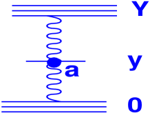
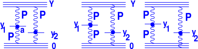
Fig.4-a	Fig. 4-b

Figure 4: The single inclusive (Fig. 4-a ) and double inclusive (Fig.4-b) cross sections in the single Pomeron exchange model in the CQM.

In the case of the single inclusive process we have only one diagram, of Fig. 4-a, all other contributions are cancelled due to the AGK cutting rules [12]. This diagram gives us

$$f_{1}(Y)\,\,=\,\,\frac{d\sigma}{dy}\,\,=\,\,18\,g_{0}^{2}\,a\,\,e^{\Delta Y};$$ (9)

we have here a combinatorial factor 9 for three quarks in each proton, and an additional factor 2. Indeed, we use the s-channel unitarity equation in the form:

$$2\,Im\,A_{el}\,=\,|\,A_{el}\,|^{2}\,+\,G_{in}\,\,,$$ (10)

and we see that for the one Pomeron exchange, which is related to the $G_{in}$ and therefore to the cut Pomeron, we have an additional 2. This will be our usual prescription for the cut Pomeron. For the double inclusive cross section we have contributions of several diagrams, given in Fig. 4-b.

1. Let us demonstrate, step by step, how to perform the calculations in this model. We have for Fig. 4-b :

   $$D_{1}(y_{1},y_{2})\,=4\,\cdot\,9\,\int\,\frac{dt}{16\,\pi}\,e^{2\,\Delta\,Y}\,e^{-|t|(4\,R^{2}_{quark}+2\alpha^{\prime}_{P}\,Y)}\,.$$ (11)

   Here 9 is a combinatorial factor, 4 comes from the AKG rules (2 for each cut Pomeron). We introduce also the constituent quark radius $R^{2}_{quark}$ in order to take into account the $t$ - dependence of the quark - Pomeron vertex, which we parametrize in the simplest Gaussian form: $g_{q-P}(t)=g_{0}\exp[R^{2}_{quark}\,t]$. Integrating this expression over $|t|$, we obtain

   $$D_{1}(y_{1},y_{2})\,=\,\frac{9}{8\,\pi}\,\frac{g_{0}^{4}\,a^{2}\,\alpha\,e^{2\,\Delta\,Y}}{\,\alpha^{\prime}_{P}\,Y\,+\,R^{2}_{quark}}.$$ (12)

2. The second diagram of Fig. 4-b is somewhat more complicated. First of all, we define the form factor for this type of diagrams:

   $$\int\,|\,\Psi\,\left(\,x_{1}\,x_{2}\,x_{3}\,\right)\,|^{2}\,\delta\left(\,\vec{x}_{1}+\vec{x}_{2}+\vec{x}_{3}\,\right)\,e^{i\,q\,x_{1}\,-i\,q\,x_{2}}\,dx_{1}\,dx_{2}\,dx_{3}\,=\,e^{-\frac{|t|}{2\,\alpha}}\,\,$$ (13)

   This gives

   $$D_{2}(y_{1},y_{2})\,=4\,\cdot\,36\,\int\,\frac{dt}{16\,\pi}\,e^{2\,\Delta\,Y}\,e^{-|t|\,2\,(\,\alpha^{\prime}_{P}\,Y\,+\,\frac{1}{2\,\alpha})}\,,$$ (14)

   where 36 is the combinatorial factor for this type of configurations, and we obtain for this diagram:

   $$D_{2}(y_{1},y_{2})\,=\,\frac{9}{\pi}\,\frac{g_{0}^{4}\,a^{2}\,\alpha\,e^{2\,\Delta\,Y}}{1+2\alpha\,\alpha^{\prime}_{P}\,Y}.$$ (15)

3. The third diagram in Fig. 4-b gives

   $$D_{3}(y_{1},y_{2})\,=4\,\cdot\,36\,\int\,\frac{dt}{16\,\pi}\,e^{2\,\Delta\,Y}\,e^{-|t|\,(2\,\alpha^{\prime}_{P}\,Y\,+\,2\,R^{2}_{quark}+\,\frac{1}{2\,\alpha})}\,.$$ (16)

   Here we used the same vertex, and after the integration we get

   $$D_{3}(y_{1},y_{2})\,=\,\frac{9}{\pi}\,\frac{g_{0}^{4}\,a^{2}\,\alpha\,e^{2\,\Delta\,Y}}{1+4\alpha\,\left(\alpha^{\prime}_{P}\,Y+\,R^{2}_{quark}\right)}.$$ (17)

Now we are ready to use our equation ( 1) and to estimate the possible dependence of $\sigma_{eff}$ on the quark radius $R^{2}_{quark}$. For the $\sigma_{eff}$ we can write

$$\sigma_{eff}\,\,=\,\,m\,\frac{f(y_{1})\,\,f(y_{2})}{2\,\left(D_{1}\left(R^{2}_{quark}\right)\,+\,D_{2}\left(R^{2}_{quark}\right)\,+\,D_{3}\,\right)}\,\,.$$ (18)

In Fig. 5 we plot the value of $\sigma_{eff}$ from Eq. (1) as a function of $R^{2}_{quark}$ for $m=1$, $y_{1}=y_{2}=Y/2$. One can see that at any value of the unknown size of the constituent quark the value of $\sigma_{eff}$ turns out to be larger than the experimental value.

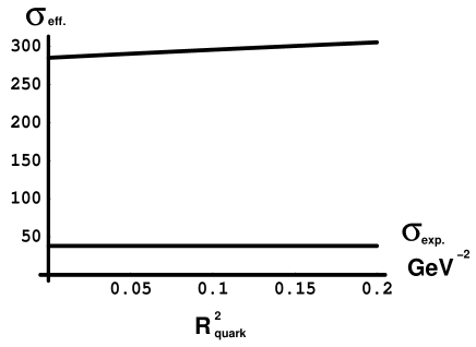
Fig.5-a	Fig. 5-b

Figure 5: $\sigma_{eff}$ (in $GeV^{-2}$) versus $R^{2}_{quark}$ (in $GeV^{-2}$) for $\alpha^{\prime}_{P}=0.25\,GeV^{-2}$ (Fig.5-a) and for $\alpha^{\prime}_{P}=0$(Fig.5-b) .The straight line in Fig. 5-b shows the experimental value of $\sigma_{eff}$.

The conclusion we derive from this simple model is quite obvious: in CQM the “soft” Pomeron exchange for quark-quark scattering cannot explain the CDF result of the double parton cross section. However, the experimental value of $\sigma_{eff}$ obtained from the high $p_{t}$ jet production can be described by a “hard” Pomeron. Indeed, in this case we have to consider $\alpha^{\prime}_{P}=0$ and Fig. 5-b shows that we have $\sigma_{eff}\,\approx\,15\,mb$ for $R^{2}_{quark}\,\approx 0.05\,GeV^{-2}$. We would like to emphasize that the double parton shower cross section $\sigma_{eff}$ is very sensitive to the size of the constituent quark in the CDF kinematics since the CDF measures the jet production by “hard” Pomeron for which $\alpha^{\prime}_{P}(0)=0$.

2.3 $\mathbf{R(t)\,\,=\,\,\frac{d\sigma^{DIS}_{el}/dt}{d\sigma^{DIS}_{inel}/dt}\,\,\,in\,\,\,the\,\,\,CQM}$

In the single Pomeron exchange model the cross section for DIS diffraction and elastic scattering can be described by two diagrams in Fig. 6.

Figure 6: The total inclusive diffraction cross section for a single Pomeron exchange in the CQM.

The first diagram in Fig. 6 leads to

$$\frac{d\sigma^{D}_{1}}{dt}\,\,=\,\,3g^{2}_{0}\,e^{2\,\Delta\,Y}\,e^{-2|t|(\alpha^{\prime}_{H}\,Y+R^{2}_{quark})}\,\,.$$ (19)

In this process the “hard” Pomeron contributes, so $\Delta=\Delta_{H}\,\approx\,0.3$ and $\alpha^{\prime}_{H}(0)=0$. It should also be stressed that the contribution of this diagram to the total cross section (integrated over $t$) is very sensitive to the value of $R_{quark}$ ($D_{1}\,\,\propto\,\,1/R^{2}_{quark}$) since this contribution is proportional to $1/(\alpha^{\prime}_{P}\,Y\,\,+\,\,R^{2}_{quark})$, and for the “hard ” Pomeron $\alpha^{\prime}_{P}(0)=0$.

Figure 7: $R(t)$ versus $t$, experimental data were taken from [1].

The second diagram in Fig. 6 depends only slightly on the value of the quark radius, and can be described as follows:

$$\frac{d\sigma^{D}_{2}}{dt}\,\,=\,\,6g^{2}_{0}\,e^{2\,\Delta\,Y}\,e^{-|t|\left(\,\frac{1}{2\alpha}\,+\,2\,(\,\alpha^{\prime}_{H}\,Y\,\,+\,\,R^{2}_{quark})\,\right)}\,\,.$$ (20)

For the elastic cross section we have

$$\frac{d\sigma^{el}_{2}}{dt}\,\,=\,\,9g^{2}_{0}\,e^{2\,\Delta\,Y}\,e^{-|t|\left(\,\frac{1}{3\alpha}\,+\,2(\,\alpha^{\prime}_{H}\,Y\,\,+\,\,R^{2}_{quark})\,\right)}\,\,.$$ (21)

Here we used the expression for the simplest form factor in this model:

$$\int\,|\,\Psi\,\left(\,x_{1}\,,x_{2}\,,x_{3}\,\right)\,|^{2}\,\delta\left(\,\vec{x_{1}}+\vec{x_{2}}+\vec{x_{3}}\,\right)\,\,e^{i\,q\,x_{1}}\,dx_{1}\,dx_{2}\,dx_{3}\,=\,e^{-\frac{|t|}{6\,\alpha}}\,\,.$$ (22)

Now we define our $d\sigma^{DIS}_{inel}/dt$ as a difference between these two contributions. Fig. 7 shows the value of the ratio $R(t)$ , given by Eq. (2). One can easily see that this ratio depends neither on the value of $R_{quark}$, nor on the value of the “hard” Pomeron intercept $\Delta$. Hence, it can be considered as a crucial test of our model.

Comparing two pictures: Fig. 5 and Fig. 7, we conclude that $\sigma_{eff}$ can be described using the small value of $R_{quark}$ and the “hard” Pomeron approach with $\alpha^{\prime}_{P}=0$, while $R$ does not depend on $R_{quark}$ and $\alpha^{\prime}_{P}=0$, and the obtained shape of R for a given t is close to the experimental graph in [1]. It follows from this simple exercise that we have to check the description of high energy scattering in the CQM including the ”triple” Pomeron vertex. But before doing this, in order to clarify the question of the possible value of triple Pomeron vertex and other parameters in this model, we will examine our model by fitting the data on total, elastic and diffractive dissociation cross sections.

2.4 Total, elastic and diffractive dissociation processes in the CQM

Let us check, how well our model, CQM, describes experimental data on total, elastic and diffractive dissociation processes. In the simplest case, without the triple Pomeron vertex corrections and additional Pomeron exchanges, we have the following contribution for the total cross section:

$$\sigma_{total}\left(\,Y\,\right)=18\,g_{0}^{2}\,e^{\Delta\,Y}\,\,.$$ (23)

Due to our s-channel unitarity constraint we write here again an additional factor two for the cut Pomeron. For the elastic cross section one can obtain

$$\sigma_{Elastic}\left(\,Y\,\right)=\frac{81}{16\,\pi}\,\frac{g_{0}^{4}\,e^{2\,\Delta\,Y}}{2\,\alpha^{\prime}_{P}\,Y\,+\,4\,R^{2}_{quark}+2/(3\,\alpha)}\,\,.$$ (24)

We define also how to calculate the diffractive dissociation process. First of all, we take into account the sum of diffractive and elastic processes. We have to calculate several types of diagrams, see Fig. 8. The answer for these diagrams is the following:

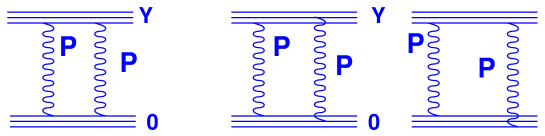
Figure 8: Diagrams for diffractive and elastic cross sections in the first order .

$$\sigma\,\left(\,Y\,\right)=\frac{9}{32\,\pi}\,\frac{g_{0}^{4}\,e^{2\,\Delta\,Y}}{\alpha^{\prime}_{P}\,Y\,+\,2\,R^{2}_{quark}}\,+\,\frac{9}{4\,\pi}\,\frac{g_{0}^{4}\,\alpha\,e^{2\,\Delta\,Y}}{1+2\,\alpha\,\alpha^{\prime}_{P}\,Y\,}\,+\,\frac{9}{2\,\pi}\,\frac{g_{0}^{4}\,\alpha\,e^{2\,\Delta\,Y}}{1+4\,\alpha\,(\alpha^{\prime}_{P}\,Y\,+\,R^{2}_{quark})}\,.$$ (25)

The experimental value of the diffractive dissociation cross section, single and double together, is equal to:

$$\sigma_{Diffr}\,\left(\,Y\,\right)\,=\,\sigma\left(\,Y\,\right)\,-\sigma_{Elastic}\left(\,Y\,\right)\,\,.$$ (26)

The result of the fitting is presented in Figs. 10 -   12. We see that we have to include into our consideration the diagrams of the next order, with the triple Pomeron vertex and with the double Pomeron exchange. Taking into account these corrections, which are given by diagrams of the type of Fig. 9, we obtain better a fit, see Figs. 10 -  12.

Figure 9: Higher order corrections.

We present the analytical expressions for these contributions in the Appendix; they are rather simple. Let us note also that we calculated both the single and double diffractive dissociation processes, and we plotted a graph with single diffractive dissociation data. Hence, it is not surprising that the obtained curve is above the experimental points. So, in this model we obtained the following parameters: for the Pomeron-quark vertex and intercept $g_{P-Q}^{2}\,=\,8\,-\,9\,GeV^{-2}$ ,$\Delta\,=\,0.08\,-\,0.09\,$, and for the value of the triple Pomeron vertex $\frac{\gamma}{{\rm g}_{0}}\,=\,0.013\,-\,0.015\,$. The conclusion is that the value of the triple Pomeron vertex is not small and the contribution of next order corrections is important.

Fig.10-a	Fig. 10-b

Figure 10: Total cross section of p-p interaction in CQM without $\gamma$, Fig.10-a, and with $\gamma$ corrections, Fig.10-b.

Fig.11-a	Fig. 11-b

Figure 11: Elastic cross section of p-p interaction in CQM without $\gamma$, Fig.11-a, and with $\gamma$ corrections, Fig.11-b.

Fig.12-a	Fig. 12-b

Figure 12: Diffractive dissociation cross section of p-p interaction in CQM without $\gamma$, Fig.12-a, and with $\gamma$ corrections, Fig.12-b.

3 Triple Pomeron interaction in CQM

In this section we are going to calculate the same processes as in the previous section, but taking into account the triple Pomeron interaction. We would like to see how this interaction changes the $R_{quark}$ dependence of the amplitude, and we will try to find a reasonable value of the quark radius to be used in the CQM based phenomenology.

3.1 $\mathbf{\sigma_{eff}}$ in one loop calculation

The triple Pomeron interaction leads to a number of new diagrams presented in Fig. 13 which we have to add to the Fig. 4 diagrams. It should be stressed that there are many diagrams which, due to the AGK cancellations [12], do not contribute to double inclusive production.

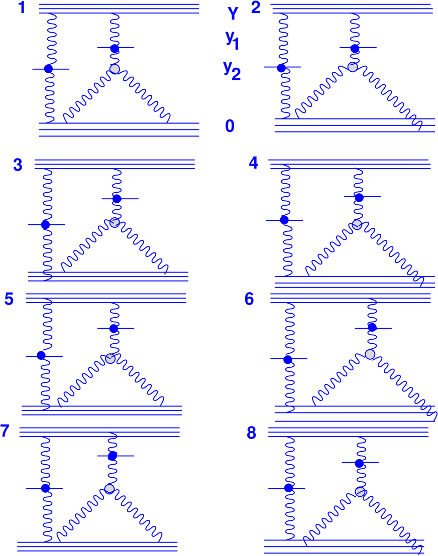
Figure 13: Diagrams incorporating the triple Pomeron interaction for $\sigma_{eff}$.

The diagrams with triple Pomeron interaction in the case of a single inclusive process are presented in Fig. 14. These diagrams are the simplest ones with the triple Pomeron vertex, which we denote by $\gamma$, and where we take $y_{1}=y_{2}=Y/2$. So, we have the following additional contributions to the single inclusive process.

1. The first diagram of Fig. 14 is

   $$f_{2}(Y)\,=\,\frac{9}{8\,\pi}\,\,g_{0}^{4}\,e^{\Delta\,Y}\,\left(\frac{\gamma}{g_{0}}\right)\,\int_{0}^{Y/2}\,\frac{dx\,e^{\Delta\,x}}{R_{quark}^{2}+\alpha^{\prime}_{P}\,x}.$$ (27)

2. The second diagram of Fig. 14 gives

   $$f_{3}(Y)\,=\,\frac{9}{\pi}\,\,g_{0}^{4}\,e^{\Delta\,Y}\,\alpha\,\left(\frac{\gamma}{g_{0}}\right)\,\int_{0}^{Y/2}\,\frac{dx\,e^{\Delta\,x}}{1+4\,\alpha\,\alpha^{\prime}_{P}\,x}.$$ (28)

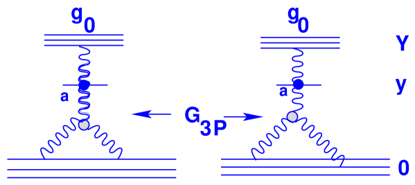
Figure 14: The diagrams with $\gamma$ contributing to the single inclusive process.

We have more complicated contributions for the double inclusive cross section. Indeed, these are all diagrams of Fig. 13 and Fig. 15. The analytical expressions for these diagrams are given in the Appendix.

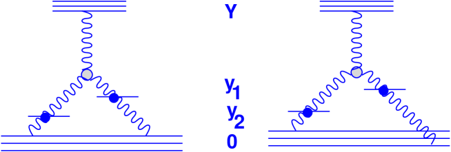
Figure 15: The simplest diagrams with $\gamma$ contributing to the double inclusive process.

Now, using Eq. (1) again, we estimate the dependence of $\sigma_{eff}$ on $R_{quark}^{2}$ in the case of one Pomeron loop. We have:

$$\sigma_{eff}\,\,=\,\,m\,\frac{\left(f_{1}(y_{1})\,+\,f_{2}(y_{1})\,+\,f_{3}(y_{1})\right)\left(f_{1}(y_{2})\,+\,f_{2}(y_{2})\,+\,f_{3}(y_{2})\right)}{2\,\left(D_{1}+D_{2}+D_{3}+D_{4}+D_{5}+D_{6}+D_{7}+D_{8}+D_{9}+D_{10}+D_{11}+D_{12}+D_{13}\right)}\,.$$ (29)

We calculate the case of symmetrical pair production, where $m=1$ and $y_{1}=y_{2}=\frac{Y}{2}$, and we take a “hard” Pomeron in this calculation, $\alpha^{\prime}_{P}=0$. We have already considered the important question of the numerical value of the triple Pomeron vertex $\gamma$. Fitting the diffraction dissociation data we obtained that $\frac{\gamma}{g_{0}}\,\sim\,0.014\,$. This is not such a small number, the one loop corrections influence and change our results. Indeed, in Fig. 16 the value of $\sigma_{eff}$ is plotted as a function $R^{2}_{quark}$, where we used Eq. 29 for the calculations.

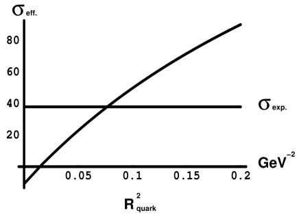
Figure 16: $\sigma_{eff}$ (in $GeV^{-2}$) versus $R^{2}_{quark}$ (in $GeV^{-2}$) for $\alpha^{\prime}_{P}=0$(Fig.5-b) .The straight line shows the experimental value of $\sigma_{eff}$.

We see that indeed, the corrections change the result, obtained in the previous calculation. However, the change is not so crucial. For a “hard” Pomeron the value of $\sigma_{eff}\,\approx\,15mb$ is achieved for $R_{quark}^{2}\,\approx\,0.08\,-\,0.07\,\,GeV^{-2}$. The conclusion is that in order to explain the CDF result for the double parton cross section we need the triple Pomeron vertex, but the value of $R_{quark}^{2}$ still remains very small.

3.2 R(t) in one loop calculation

In the case of triple Pomeron interaction we have an additional number of diagrams which contribute to the elastic cross section of DIS and to the inelastic diffraction in DIS. First of all, consider the diagrams of DIS, presented in Figs. 17 and  18, which describe elastic and proton diffraction processes together. The expressions corresponding to these diagrams are also presented in the Appendix.

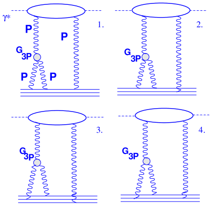
Figure 17: The $\gamma$ corrections to the inelastic diffraction in DIS .

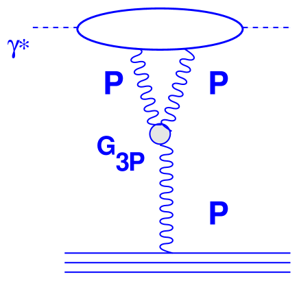
Figure 18: Inelastic diffraction diagram in DIS .

In these diagrams we defined by $\Delta_{S}\,\approx\,0.08$ and $\alpha^{\prime}_{P}\,\approx\,0.2$ the intercept and the slope of the “soft” Pomeron, and by $\Delta\,\approx\,0.3$ and $\alpha^{\prime}_{H}\,\approx\,0$ the intercept and the slope of the “hard” Pomeron. We also introduced $\tilde{\Delta}\,=\,2\,\Delta_{S}\,-\,\Delta$.

The calculation of the elastic cross section in DIS for one loop leads to:

$$\frac{d\sigma^{el}_{2}}{dt}\,\,=-\,\,\frac{9}{8\,\pi}g^{4}_{0}\,e^{2\,\Delta\,Y}\,\left(\frac{\gamma}{g_{0}}\right)\,\int_{0}^{Y}\,\frac{dx\,e^{\tilde{\Delta}\,x}}{\alpha^{\prime}_{P}\,x\,+\,\frac{1}{4\,\alpha}}\,e^{-|t|(2\,\alpha^{\prime}_{H}\,Y+R^{2}_{quark}-\,\alpha^{\prime}_{H}\,x\,+\frac{\alpha^{\prime}_{P}\,x}{2}+\frac{7}{24\,\alpha})}\,-$$

$$-\frac{9}{16\,\pi}g^{4}_{0}\,e^{2\,\Delta\,Y}\,\left(\frac{\gamma}{g_{0}}\right)\,\int_{0}^{Y}\,\frac{dx\,e^{\tilde{\Delta}\,x}}{\alpha^{\prime}_{P}\,x\,+\,R_{quark}^{2}}\,e^{-|t|(2\,\alpha^{\prime}_{H}\,Y+\frac{3\,R^{2}_{quark}}{2}-\,\alpha^{\prime}_{H}\,x\,+\frac{\alpha^{\prime}_{P}\,x}{2}+\frac{1}{6\,\alpha})}\,\,.$$ (30)

Here $\frac{d\sigma^{DIS}_{inel}}{dt}$ is considered as the difference between the contributions of diagrams of Figs. 17,  18 and of the elastic cross section. Now we are ready get the ratio $R(t)$, which is given by Eq. (2). The result is shown in Fig. 19-a. Actually, there is a fast exponential fall of the curve, due the parametrization chosen for our vertices. Therefore we present also the graph Fig. 19-b, where, instead of the simplest Gaussian parametrization $e^{t\,R^{2}_{quark}}$, we introduce a more realistic form factor $F_{elastic}(|t|)=1/(1\,+\,|t|\,/\,0.72\,)^{2}$ for the calculation of the elastic cross section. For the calculation of the diffraction dissociation cross section we also take a different form factor $F_{diffr}(|t|)=1/(1\,+\,|t|/2\alpha)$, which is the first term of the expansion of $e^{-|t|/2\alpha}$, which we used before as the parametrization for the form factor in the case of diffractive dissotiacion at the “tree” level.

We see, that we obtain here a better fit.

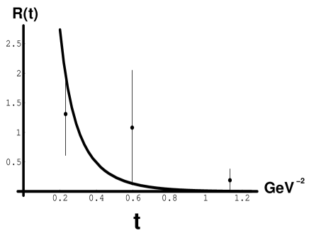
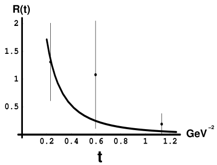
Fig.19-a	Fig. 19-b

Figure 19: $R(t)$ versus t in one loop calculation for the case of our parametrization of the Pomeron-quark interaction vertex, Fig.19-a and for the case of a more realistic parameterization, Fig.19-b.

The obtained result for the one loop calculation is, in this simplest estimations, not so different from the “tree” calculation, in spite of the fact that in one loop calculation the radius of the quark, $R^{2}_{quark}\approx\,0.08\,-\,0.1\,\,GeV^{-2}$ is involved. And it seems that in the order to obtain a better fit to this data, we have to consider corrections, where more realistic form factors will be taken into account.

4 Conclusion

In this paper we demonstrate that the new beautiful experimental data on double parton shower effective cross section (CDF, Tevatron) and on the ratio of elastic and inelastic diffraction production in DIS (ZEUS, HERA) can be described in the framework of the naive Constituent Quark Model (CQM). The value of the quark radius turns out to be small: it is equal to $R^{2}_{quark}\,=\,0.07-\,0.1\,GeV^{-2}$. This smallness can be considered as an argument supporting the idea that constituent quarks are the correct degrees of freedom for soft (long distance) interactions. It should be stressed also that we reached a satisfactory description of the experimental data by introducing only the triple Pomeron interaction. This means that the constituent quarks do not exhaust all degrees of freedom of soft high energy interaction. Much work is needed to build a comprehensive theoretical approach for long distance interaction and we consider the fact that the CQM describes all data of soft interaction, as our small contribution to the solution of this complicated problem.

5 Acknowledgments

We would like to thank Asher Gotsman, Uri Maor and Eran Naftali for many informative and encouraging discussions on the sabject of this paper. The research of S.B. and E.L. was supported in part by the GIF grant # I-620-22.14/1994, by the BSF grant # 9800276 and by the Israel Science Foundation founded by the Israeli Academy of Science and Humanities.

Appendix

Appendix A The next order corrections

The next order corrections are the corrections where the double Pomeron exchange and triple Pomeron vertex are included. In the case of the total cross section there are the following additional contributions:

$$\sigma_{total}^{1}\,\left(\,Y\,\right)=-\frac{9}{32\,\pi}\,\frac{g_{0}^{4}\,e^{2\,\Delta\,Y}}{\alpha^{\prime}_{P}\,Y\,+\,2\,R^{2}_{quark}}\,-\,\frac{9}{4\,\pi}\,\frac{g_{0}^{4}\,\alpha\,e^{2\,\Delta\,Y}}{1+2\,\alpha\,\alpha^{\prime}_{P}\,Y\,}\,-\,\frac{9}{2\,\pi}\,\frac{g_{0}^{4}\,\alpha\,e^{2\,\Delta\,Y}}{1+4\,\alpha\,(\alpha^{\prime}_{P}\,Y\,+\,R^{2}_{quark})}\,-\,$$

$$\,\frac{9}{8\,\pi}\,\,g_{0}^{4}\,e^{\Delta\,Y}\,\left(\frac{\gamma}{g_{0}}\right)\,\int_{0}^{Y}\,\frac{dx\,e^{\Delta\,x}}{R_{quark}^{2}+\alpha^{\prime}_{P}\,x}-\,\frac{9}{\pi}\,\,g_{0}^{4}\,e^{\Delta\,Y}\,\alpha\,\left(\frac{\gamma}{g_{0}}\right)\,\int_{0}^{Y/2}\,\frac{dx\,e^{\Delta\,x}}{1+4\,\alpha\,\alpha^{\prime}_{P}\,x}\,\,+$$

$$\,\frac{9}{128\,\pi^{2}}\,\,g_{0}^{6}\,e^{2\,\Delta\,Y}\,\left(\frac{\gamma}{g_{0}}\right)\,\int_{0}^{Y}\,\frac{dx\,e^{\Delta\,x}}{\left(2\,\alpha^{\prime}\,Y+\frac{7\,R_{quark}^{2}}{2}-\frac{\alpha^{\prime}_{P}\,x}{2}\right)\,\left(R_{quark}^{2}+\alpha^{\prime}_{P}\,x\right)}\,+$$

$$\,\frac{9}{64\,\pi^{2}}\,\,g_{0}^{6}\,e^{2\,\Delta\,Y}\,\left(\frac{\gamma}{g_{0}}\right)\,\int_{0}^{Y}\,\frac{dx\,e^{\Delta\,x}}{\left(2\,\alpha^{\prime}\,Y+\frac{7\,R_{quark}^{2}}{2}-\frac{\alpha^{\prime}_{P}\,x}{2}+\frac{1}{2\,\alpha}\right)\,\left(R_{quark}^{2}+\alpha^{\prime}_{P}\,x\right)}\,+$$

$$\,\frac{9}{32\,\pi^{2}}\,\,g_{0}^{6}\,e^{2\,\Delta\,Y}\,\left(\frac{\gamma}{g_{0}}\right)\,\int_{0}^{Y}\,\frac{dx\,e^{\Delta\,x}}{\left(4\,\alpha^{\prime}\,Y+3\,R_{quark}^{2}-\alpha^{\prime}_{P}\,x+\frac{1}{\alpha}\right)\,\left(R_{quark}^{2}+\alpha^{\prime}_{P}\,x\right)}\,+$$

$$\,\frac{9}{16\,\pi^{2}}\,\,g_{0}^{6}\,e^{2\,\Delta\,Y}\,\left(\frac{\gamma}{g_{0}}\right)\,\int_{0}^{Y}\,\frac{dx\,e^{\Delta\,x}}{\left(4\,\alpha^{\prime}\,Y+3\,R_{quark}^{2}-\alpha^{\prime}_{P}\,x+\frac{3}{2\,\alpha}\right)\,\left(R_{quark}^{2}+\alpha^{\prime}_{P}\,x\right)}\,+$$

$$\,\frac{9}{64\,\pi^{2}}\,\,g_{0}^{6}\,e^{2\,\Delta\,Y}\,\left(\frac{\gamma}{g_{0}}\right)\,\int_{0}^{Y}\,\frac{dx\,e^{\Delta\,x}}{\left(\left(3\,R_{quark}^{2}+2\,\alpha^{\prime}_{P}\,Y\right)\left(\frac{1}{4\,\alpha}+\alpha^{\prime}_{P}\,x\right)-\frac{\alpha^{{}^{\prime}2}_{P}\,x^{2}}{2}\right)}\,-$$

$$\,\frac{9}{64\,\pi^{2}}\,\,g_{0}^{6}\,e^{2\,\Delta\,Y}\,\left(\frac{\gamma}{g_{0}}\right)\,\int_{0}^{Y}\,\frac{dx\,e^{\Delta\,x}}{\left(2\,\alpha^{\prime}\,Y+2\,R_{quark}^{2}-\frac{\alpha^{\prime}_{P}\,x}{2}+\frac{3}{8\,\alpha}\right)\,\left(\frac{1}{4\,\alpha}+\alpha^{\prime}_{P}\,x\right)}\,+$$

$$\,\frac{9}{32\,\pi^{2}}\,\,g_{0}^{6}\,e^{2\,\Delta\,Y}\,\left(\frac{\gamma}{g_{0}}\right)\,\int_{0}^{Y}\,\frac{dx\,e^{\Delta\,x}}{\left(2\,\alpha^{\prime}_{P}\,Y-\frac{\alpha^{\prime}_{P}\,x}{2}+\frac{7}{8\,\alpha}\right)\,\left(\frac{1}{4\,\alpha}+\alpha^{\prime}_{P}\,x\right)}\,+$$

$$\,\frac{9}{32\,\pi^{2}}\,\,g_{0}^{6}\,e^{2\,\Delta\,Y}\,\left(\frac{\gamma}{g_{0}}\right)\,\int_{0}^{Y}\,\frac{dx\,e^{\Delta\,x}}{\left(\left(R_{quark}^{2}+2\,\alpha^{\prime}_{P}\,Y+\frac{1}{2\,\alpha}\right)\left(\frac{1}{4\,\alpha}+\alpha^{\prime}_{P}\,x\right)-\frac{\alpha^{{}^{\prime}2}_{P}\,x^{2}}{2}\right)}\,.$$ (31)

For the elastic cross section we have in the next order:

$$\sigma_{Elastic}^{1}\,\left(\,Y\,\right)=-\,\frac{81}{128\,\pi^{2}}\,\,g_{0}^{6}\,e^{2\,\Delta\,Y}\,\left(\frac{\gamma}{g_{0}}\right)\,\int_{0}^{Y}\,\frac{dx\,e^{\Delta\,x}}{\left(2\,\alpha^{\prime}\,Y+\frac{3\,R_{quark}^{2}}{2}-\frac{\alpha^{\prime}_{P}\,x}{2}+\frac{1}{6\,\alpha}\right)\,\left(R_{quark}^{2}+\alpha^{\prime}_{P}\,x\right)}\,-$$

$$\,\frac{81}{64\,\pi^{2}}\,\,g_{0}^{6}\,e^{2\,\Delta\,Y}\,\left(\frac{\gamma}{g_{0}}\right)\,\int_{0}^{Y}\,\frac{dx\,e^{\Delta\,x}}{\left(2\,\alpha^{\prime}\,Y+R_{quark}^{2}-\frac{\alpha^{\prime}_{P}\,x}{2}+\frac{13}{24\,\alpha}\right)\,\left(\frac{1}{4\,\alpha}+\alpha^{\prime}_{P}\,x\right)}\,.$$ (32)

And for sum of elastic and diffractive dissotiation cross sections we have:

$$\sigma_{Elastic+diffr}^{1}\,\left(\,Y\,\right)=\,\frac{9}{8\,\pi}\,\,g_{0}^{4}\,e^{\Delta\,Y}\,\left(\frac{\gamma}{g_{0}}\right)\,\int_{0}^{Y}\,\frac{dx\,e^{\Delta\,x}}{R_{quark}^{2}+\alpha^{\prime}_{P}\,x}.+\,\frac{9}{\pi}\,\,g_{0}^{4}\,e^{\Delta\,Y}\,\alpha\,\left(\frac{\gamma}{g_{0}}\right)\,\int_{0}^{Y/2}\,\frac{dx\,e^{\Delta\,x}}{1+4\,\alpha\,\alpha^{\prime}_{P}\,x}\,\,-$$

$$\,\frac{27}{128\,\pi^{2}}\,\,g_{0}^{6}\,e^{2\,\Delta\,Y}\,\left(\frac{\gamma}{g_{0}}\right)\,\int_{0}^{Y}\,\frac{dx\,e^{\Delta\,x}}{\left(2\,\alpha^{\prime}\,Y+\frac{7\,R_{quark}^{2}}{2}-\frac{\alpha^{\prime}_{P}\,x}{2}\right)\,\left(R_{quark}^{2}+\alpha^{\prime}_{P}\,x\right)}\,-$$

$$\,\frac{27}{64\,\pi^{2}}\,\,g_{0}^{6}\,e^{2\,\Delta\,Y}\,\left(\frac{\gamma}{g_{0}}\right)\,\int_{0}^{Y}\,\frac{dx\,e^{\Delta\,x}}{\left(2\,\alpha^{\prime}\,Y+\frac{7\,R_{quark}^{2}}{2}-\frac{\alpha^{\prime}_{P}\,x}{2}+\frac{1}{2\,\alpha}\right)\,\left(R_{quark}^{2}+\alpha^{\prime}_{P}\,x\right)}\,-$$

$$\,\frac{27}{32\,\pi^{2}}\,\,g_{0}^{6}\,e^{2\,\Delta\,Y}\,\left(\frac{\gamma}{g_{0}}\right)\,\int_{0}^{Y}\,\frac{dx\,e^{\Delta\,x}}{\left(4\,\alpha^{\prime}\,Y+3\,R_{quark}^{2}-\alpha^{\prime}_{P}\,x+\frac{1}{\alpha}\right)\,\left(R_{quark}^{2}+\alpha^{\prime}_{P}\,x\right)}\,-$$

$$\,\frac{27}{16\,\pi^{2}}\,\,g_{0}^{6}\,e^{2\,\Delta\,Y}\,\left(\frac{\gamma}{g_{0}}\right)\,\int_{0}^{Y}\,\frac{dx\,e^{\Delta\,x}}{\left(4\,\alpha^{\prime}\,Y+3\,R_{quark}^{2}-\alpha^{\prime}_{P}\,x+\frac{3}{2\,\alpha}\right)\,\left(R_{quark}^{2}+\alpha^{\prime}_{P}\,x\right)}\,-$$

$$\,\frac{27}{64\,\pi^{2}}\,\,g_{0}^{6}\,e^{2\,\Delta\,Y}\,\left(\frac{\gamma}{g_{0}}\right)\,\int_{0}^{Y}\,\frac{dx\,e^{\Delta\,x}}{\left(\left(3\,R_{quark}^{2}+2\,\alpha^{\prime}_{P}\,Y\right)\left(\frac{1}{4\,\alpha}+\alpha^{\prime}_{P}\,x\right)-\frac{\alpha^{{}^{\prime}2}_{P}\,x^{2}}{2}\right)}\,-$$

$$\,\frac{27}{64\,\pi^{2}}\,\,g_{0}^{6}\,e^{2\,\Delta\,Y}\,\left(\frac{\gamma}{g_{0}}\right)\,\int_{0}^{Y}\,\frac{dx\,e^{\Delta\,x}}{\left(2\,\alpha^{\prime}\,Y+2\,R_{quark}^{2}-\frac{\alpha^{\prime}_{P}\,x}{2}+\frac{3}{8\,\alpha}\right)\,\left(\frac{1}{4\,\alpha}+\alpha^{\prime}_{P}\,x\right)}\,-$$

$$\,\frac{27}{32\,\pi^{2}}\,\,g_{0}^{6}\,e^{2\,\Delta\,Y}\,\left(\frac{\gamma}{g_{0}}\right)\,\int_{0}^{Y}\,\frac{dx\,e^{\Delta\,x}}{\left(2\,\alpha^{\prime}_{P}\,Y-\frac{\alpha^{\prime}_{P}\,x}{2}+\frac{7}{8\,\alpha}\right)\,\left(\frac{1}{4\,\alpha}+\alpha^{\prime}_{P}\,x\right)}\,-$$

$$\,\frac{27}{32\,\pi^{2}}\,\,g_{0}^{6}\,e^{2\,\Delta\,Y}\,\left(\frac{\gamma}{g_{0}}\right)\,\int_{0}^{Y}\,\frac{dx\,e^{\Delta\,x}}{\left(\left(R_{quark}^{2}+2\,\alpha^{\prime}_{P}\,Y+\frac{1}{2\,\alpha}\right)\left(\frac{1}{4\,\alpha}+\alpha^{\prime}_{P}\,x\right)-\frac{\alpha^{{}^{\prime}2}_{P}\,x^{2}}{2}\right)}\,.$$ (33)

Appendix B Diagrams which contribute to the double inclusive cross section

1. First diagram of Fig. 15:

   $$D_{4}(Y)\,=\,\frac{9}{4\,\pi}\,\,g_{0}^{4}\,e^{\Delta\,Y}\,\left(\frac{\gamma}{g_{0}}\right)\,\int^{Y}_{Y/2}\,\frac{dx\,e^{\Delta\,x}}{R_{quark}^{2}+\alpha^{\prime}_{P}\,x}.$$ (34)

2. Second diagram of Fig. 15:

   $$D_{5}(Y)\,=\,\frac{18}{\pi}\,\,g_{0}^{4}\,e^{\Delta\,Y}\,\alpha\,\left(\frac{\gamma}{g_{0}}\right)\,\int^{Y}_{Y/2}\,\frac{dx\,e^{\Delta\,x}}{1+4\alpha\,\alpha^{\prime}_{P}\,x}.$$ (35)

3. First diagram of Fig. 13

   $$D_{6}(Y)\,=-\,\frac{9}{64\,\pi^{2}}\,\,g_{0}^{6}\,e^{2\,\Delta\,Y}\,\left(\frac{\gamma}{g_{0}}\right)\,\int_{0}^{Y/2}\,\frac{dx\,e^{\Delta\,x}}{\left(2\,\alpha^{\prime}\,Y+\frac{7\,R_{quark}^{2}}{2}-\frac{\alpha^{\prime}_{P}\,x}{2}\right)\,\left(R_{quark}^{2}+\alpha^{\prime}_{P}\,x\right)}.$$ (36)

4. Second diagram of Fig. 13 gives

   $$D_{7}(y)\,=-\,\frac{9}{32\,\pi^{2}}\,\,g_{0}^{6}\,e^{2\,\Delta\,Y}\,\left(\frac{\gamma}{g_{0}}\right)\,\int_{0}^{Y/2}\,\frac{dx\,e^{\Delta\,x}}{\left(2\,\alpha^{\prime}\,Y+\frac{7\,R_{quark}^{2}}{2}-\frac{\alpha^{\prime}_{P}\,x}{2}+\frac{1}{2\,\alpha}\right)\,\left(R_{quark}^{2}+\alpha^{\prime}_{P}\,x\right)}.$$ (37)

5. Third diagram of Fig. 13 gives

   $$D_{8}(Y)\,=-\,\frac{9}{16\,\pi^{2}}\,\,g_{0}^{6}\,e^{2\,\Delta\,Y}\,\left(\frac{\gamma}{g_{0}}\right)\,\int_{0}^{Y/2}\,\frac{dx\,e^{\Delta\,x}}{\left(4\,\alpha^{\prime}\,Y+3\,R_{quark}^{2}-\alpha^{\prime}_{P}\,x+\frac{1}{\alpha}\right)\,\left(R_{quark}^{2}+\alpha^{\prime}_{P}\,x\right)}.$$ (38)

6. Fourth diagram of Fig. 13

   $$D_{9}(Y)\,=-\,\frac{9}{8\,\pi^{2}}\,\,g_{0}^{6}\,e^{2\,\Delta\,Y}\,\left(\frac{\gamma}{g_{0}}\right)\,\int_{0}^{Y/2}\,\frac{dx\,e^{\Delta\,x}}{\left(4\,\alpha^{\prime}\,Y+3\,R_{quark}^{2}-\alpha^{\prime}_{P}\,x+\frac{3}{2\,\alpha}\right)\,\left(R_{quark}^{2}+\alpha^{\prime}_{P}\,x\right)}.$$ (39)

7. Fifth diagram of Fig. 13

   $$D_{10}(Y)\,=-\,\frac{9}{32\,\pi^{2}}\,\,g_{0}^{6}\,e^{2\,\Delta\,Y}\,\left(\frac{\gamma}{g_{0}}\right)\,\int_{0}^{Y/2}\,\frac{dx\,e^{\Delta\,x}}{\left(\left(3\,R_{quark}^{2}+2\,\alpha^{\prime}_{P}\,Y\right)\left(\frac{1}{4\,\alpha}+\alpha^{\prime}_{P}\,x\right)-\frac{\alpha^{{}^{\prime}2}_{P}\,x^{2}}{2}\right)}.$$ (40)

8. Sixth diagram of Fig. 13

   $$D_{11}(Y)\,=-\,\frac{9}{32\,\pi^{2}}\,\,g_{0}^{6}\,e^{2\,\Delta\,Y}\,\left(\frac{\gamma}{g_{0}}\right)\,\int_{0}^{Y/2}\,\frac{dx\,e^{\Delta\,x}}{\left(2\,\alpha^{\prime}\,Y+2\,R_{quark}^{2}-\frac{\alpha^{\prime}_{P}\,x}{2}+\frac{3}{8\,\alpha}\right)\,\left(\frac{1}{4\,\alpha}+\alpha^{\prime}_{P}\,x\right)}.$$ (41)

9. Seventh diagram of Fig. 13

   $$D_{12}(Y)\,=-\,\frac{9}{16\,\pi^{2}}\,\,g_{0}^{6}\,e^{2\,\Delta\,Y}\,\left(\frac{\gamma}{g_{0}}\right)\,\int_{0}^{Y/2}\,\frac{dx\,e^{\Delta\,x}}{\left(2\,\alpha^{\prime}_{P}\,Y-\frac{\alpha^{\prime}_{P}\,x}{2}+\frac{7}{8\,\alpha}\right)\,\left(\frac{1}{4\,\alpha}+\alpha^{\prime}_{P}\,x\right)}.$$ (42)

10. Eighth diagram of Fig. 13

    $$D_{13}(Y)\,=-\,\frac{9}{16\,\pi^{2}}\,\,g_{0}^{6}\,e^{2\,\Delta\,Y}\,\left(\frac{\gamma}{g_{0}}\right)\,\int_{0}^{Y/2}\,\frac{dx\,e^{\Delta\,x}}{\left(\left(R_{quark}^{2}+2\,\alpha^{\prime}_{P}\,Y+\frac{1}{2\,\alpha}\right)\left(\frac{1}{4\,\alpha}+\alpha^{\prime}_{P}\,x\right)-\frac{\alpha^{{}^{\prime}2}_{P}\,x^{2}}{2}\right)}.$$ (43)

Appendix C Diagrams wich contribute to the total inelastic diffraction in DIS

1. The first diagram of Fig. 17 gives

   $$\frac{d\sigma^{D}_{3}}{dt}\,\,=-\,\,\frac{3}{16\,\pi}g^{4}_{0}\,e^{2\,\Delta\,Y}\,\left(\frac{\gamma}{g_{0}}\right)\,\int_{0}^{Y}\,\frac{dx\,e^{\tilde{\Delta}\,x}}{\alpha^{\prime}_{P}\,x\,+\,R_{quark}^{2}}\,e^{-|t|(2\,\alpha^{\prime}_{H}\,Y+\frac{3\,R^{2}_{quark}}{2}-\,\alpha^{\prime}_{H}\,x\,+\frac{\alpha^{\prime}_{P}\,x}{2})}\,\,.$$ (44)

2. From second diagram of Fig. 17 we obtain

   $$\frac{d\sigma^{D}_{4}}{dt}\,\,=-\,\,\frac{3}{8\,\pi}g^{4}_{0}\,e^{2\,\Delta\,Y}\,\left(\frac{\gamma}{g_{0}}\right)\,\int_{0}^{Y}\,\frac{dx\,e^{\tilde{\Delta}\,x}}{\alpha^{\prime}_{P}\,x\,+\,R_{quark}^{2}}\,e^{-|t|(2\,\alpha^{\prime}_{H}\,Y+\frac{3\,R^{2}_{quark}}{2}-\,\alpha^{\prime}_{H}\,x\,+\frac{\alpha^{\prime}_{P}\,x}{2}+\frac{1}{2\,\alpha})}\,\,.$$ (45)

3. Third diagram of Fig. 17

   $$\frac{d\sigma^{D}_{5}}{dt}\,\,=-\,\,\frac{3}{8\,\pi}g^{4}_{0}\,e^{2\,\Delta\,Y}\,\left(\frac{\gamma}{g_{0}}\right)\,\int_{0}^{Y}\,\frac{dx\,e^{\tilde{\Delta}\,x}}{\alpha^{\prime}_{P}\,x\,+\,\frac{1}{4\,\alpha}}\,e^{-|t|(2\,\alpha^{\prime}_{H}\,Y+R^{2}_{quark}-\,\alpha^{\prime}_{H}\,x\,+\frac{\alpha^{\prime}_{P}\,x}{2}+\frac{3}{8\,\alpha})}\,\,.$$ (46)

4. Fourth diagram of Fig. 17 gives

   $$\frac{d\sigma^{D}_{6}}{dt}\,\,=-\,\,\frac{3}{8\,\pi}g^{4}_{0}\,e^{2\,\Delta\,Y}\,\left(\frac{\gamma}{g_{0}}\right)\,\int_{0}^{Y}\,\frac{dx\,e^{\tilde{\Delta}\,x}}{\alpha^{\prime}_{P}\,x\,+\,\frac{1}{4\,\alpha}}\,e^{-|t|(2\,\alpha^{\prime}_{H}\,Y+R^{2}_{quark}-\,\alpha^{\prime}_{H}\,x\,+\frac{\alpha^{\prime}_{P}\,x}{2}+\frac{1}{8\,\alpha}-\frac{1}{8\,\alpha+32\,\alpha^{2}\,\alpha^{\prime}_{P}\,x})}\,\,,$$ (47)

5. And the last diagram of Fig. 18 leads to:

   $$\frac{d\sigma^{D}_{7}}{dt}\,\,=6\,g^{2}_{0}\,\left(\frac{\gamma}{g_{0}}\right)\,e^{-|t|\,R^{2}_{quark}}\,\frac{1\,-\,e^{-(2\Delta-\Delta_{S})\,Y}}{2\Delta-\Delta_{S}}\,\,.$$ (48)

References

-
[1]
K. Goulianos, Nucl. Phys. Proc. Suppl. 99 (2001) 37;
E. A. De Wolf, “Diffractive scattering,” hep-ph/0203074,Talk given at New Trends in HERA Physics 2001, Ringberg Castle, Tegernsee, Germany, 17-22 Jun 2001;
H. Kowalski, “Inclusive Diffraction at HERA”, p.361, G. Grindhammer, B.A. Kniehl and G. Kramer (Eds.), “New Trends in HERA Physics 1999”, Springer 1999, Ringberg Workshop, 30 May - 4 June, Tegernsee, Germany;
K. Mauritz, “Hard Diffraction at the Tevatron”, p.381, G. Grindhammer, B.A. Kniehl and G. Kramer (Eds.), “New Trends in HERA Physics 1999”, Springer 1999, Ringberg Workshop, 30 May - 4 June, Tegernsee, Germany;
H. Abramowicz and A. Caldwell, Rev.Mod.Phys. 71 (1999) 1275;
J.Breitweg et.al., ZEUS collobaration, HERA : DESY 99-160;
K. Goulianos, Phys. Rep. 101 (1983) 171; A. B. Kaidalov, Phys. Rep. 50 (1979) 157. - [2] A. H. Mueller, Nucl. Phys. B335 (1990) 115.
-
[3]
A. Zamolodchikov, B. Kopeliovich and L. Lapidus, JETP Lett. 33
(1981) 595;
E.M. Levin and M.G. Ryskin, Sov. J. Nucl. Phys. 45 (1987) 150. -
[4]
E. Levin and L. Frankfurt, JETP Lett. 2 (1965) 65;
H. J. Lipkin and F. Scheck, Phys. Rev. Lett. 16 (1966) 71. -
[5]
J.J.J. Kokkedee, “ The Quark Model”, NY, W.A. Benjamin, 1969;
V.V. Anisovich, M.N. Kobrinsky, J. Nyiri and Yu.M. Shabelski, “Quark model and high energy collisions” , WS, Singapore (1985);
V.M. Braun and Yu.M. Shabelski, Int.J.Mod.Phys. A3 (1988) 2417. - [6] T.Shfer, E.V.Shuryak, Rev.Mod.Phys. 70 (1998) 323 and references therein.
-
[7]
O.Nachtmann, “ High Energy Collisions and Nonperturbative QCD”,
HP-THEP-96-38, hep-ph/9609365 and references
therein;
H. G. Dosch, “Space-Time Picture Of High Energy Scattering”, in Shifman, M. (ed.): “At the frontier of particle physics”, vol. 2, pp. 1195-1236;
A. Donnachie and H G Dosch, Phys.Rev. D65 (2002) 014019, H.G. Dosch, O. Nachtmann, T. Paulus and S. Weinstock, Eur.Phys.J. C21 (2001) 339, H. G. Dosch, Acta Phys.Polon. B30 (1999) 3813-3835 and references therein. - [8] F.Abe et.al., The CDF Collaboration: FERMILAB-PUB-97/083-E.
-
[9]
A. M. Cooper-Sarkar, R. C. E. Devenish and A. De Roeck, Int. J. Mod.
Phys. A13 (1998) 33;
H. Abramowicz and A. Caldwell, Rev.Mod.Phys. 71 (1999) 1275;
H1 Collaboration: C. Adloff et al., Z. Phys. C76:97 (613); Phys. Lett. B483(2000) 36;
ZEUS Collaboration: J. Breitweg et al., Eur. Phys. J. C6 (1999) 43; Eur. Phys. J. C14 (2000) 213. -
[10]
. B. Kaidalov,
“Regge poles in QCD”, hep-ph/0103011 Shifman, M.
(ed.): At the frontier of particle physics”, vol. 1,pp.
603-636;
E. Levin, ”Everything about Reggeons”, DESY 97-213 , hep-ph/9710546 and references therein;
L. Caneschi (ed): “ Regge Theory of Low - Hadronic Reactions”, North-Holland, 1989. - [11] A.H. Mueller, Phys. Rev. D2 (1970) 2963; D4 (1971) 855.
- [12] V.A. Abramovsky, V.N. Gribov and O,V. Kancheli, Sov. J. Nucl. Phys. 18 (1973) 308.
- [13] A. Donnachie, P. V. Landshoff, Phys. Lett. B296 (1992) 227; B437(1998) 408 and references therein.
-
[14]
L. V. Gribov,
E. M. Levin and M. G. Ryskin, Phys.Rep. 100, 1 (1983);
A. H. Mueller and J.-W. Qiu, Nucl. Phys. B268 (1986) 427;
L. McLerran and R. Venogopalan, Phys. Rev. D49 (1994) 2233, 3352.