ON THE INFLUENCE OF EINSTEIN–PODOLSKY–ROSEN EFFECT ON THE DOMAIN WALL FORMATION
DURING THE COSMOLOGICAL PHASE TRANSITIONS

Abstract. Search for the mechanisms suppressing formation of Higgs field defects (e.g. domain walls) during the cosmological phase transitions is one of key problems in explanation of the observed large-scale uniformity of the space–time. One of the possible solutions can be based on accounting for Einstein–Podolsky–Rosen (EPR) correlations. Namely, if a coherent quantum state of the Higgs field was formed in the course of its previous evolution, then reduction to the state with broken symmetry during the phase transition should be correlated even at the scales exceeding the local cosmological horizons. Detailed consideration of the simplest one-dimensional cosmological model with $Z_{2}$ Higgs field demonstrates that, at certain parameters of the Lagrangian, EPR-correlations really result in a substantial suppression of spontaneous formation of the domain walls.

1 History and Present-Day Status of the Domain Wall Problem
in Cosmology

The first mention about the problem of domain walls in field theories with spontaneous symmetry breaking was done by Bogoliubov at the conference held in Pisa (Italy) in 1964. As was written later in his report $\!{{\bf??}}$, “it is hard to admit, for example, that the ‘phases’ are the same everywhere in the space. So it appears necessary to consider such things as ‘domain structure’ of the vacuum.”

The next important step was done about 10 years later by Zel’dovich, Kobzarev, and Okun $\!{{\bf??}}$, who presented a first detailed consideration of the role of domain walls in the astrophysical context and pointed both to the positive aspects and difficulties arising in the cosmological models involving spontaneous symmetry breaking.

At last, the problem of domain walls and other Higgs field defects became one of the central topics of cosmology in the early 1980s, after appearance of the inflationary models, whose first versions were substantially based on the dynamics of Higgs fields in the course of their phase transitions. One of the principal difficulties of such models was associated with the fact that the observed region of the Universe consists of a large number of subregions that were causally-disconnected during the phase transition. Their stable vacuum states, in general, should be different and, therefore, separated by the domain walls, involving considerable energy density. But subsequent evolution and decay of these domain walls should result in dramatic irregularity of the space–time, contradicting to observational data.

Even after development of the “new” and “chaotic” inflation scenarios $\!{{\bf??}}$, which avoid the domain wall formation at the earliest stages of cosmological evolution, this problem still remains important for the phase transitions occurring at the later times and less energies.

Moreover, the problem of domain walls became even more pressing in the late 1990s, when detailed measurements of fluctuations in the cosmic microwave background radiation (CMBR) pointed to the absence of contribution to the large-scale structure from the processes of disintegration of Higgs field defects.

There is a quite large number of works aimed at solving the above-mentioned problem. Unfortunately, their most objectionable feature is introduction of some arbitrary modifications to the theory of elementary particles, having no experimental (laboratory) confirmations. The main aim of the present report is to describe an alternative approach, which is based on accounting for EPR correlations and can be justified by, at least, some indirect laboratory experiments.

2 EPR Correlations and Macroscopic Quantum Phenomena:
Their Probable Role in Cosmology

In the general case, Einstein–Podolsky–Rosen (EPR) effect $\!{{\bf??}}$ can be defined as a correlated character of quantum processes in the “causally-disconnected” (i.e., separated by a space-like interval) regions provided that they refer to a single (coherent) quantum state of the system. The simplest and most well-known example is a correlated measurement of the polarization states of two photons emitted by the same source, as shown in the left panel of Fig. 1.

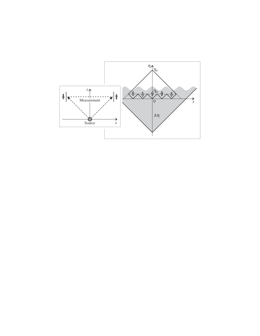
Figure 1: A scheme of laboratory EPR experiment (left panel) and conformal diagram of the space–time involving a phase transition of Higgs field (right panel).

Moreover, there are some indirect experimental evidences (the most remarkable of which were obtained in the recent years) pointing to a possibility of EPR correlations even in macroscopic systems. Particularly, we should mention
(1) the quantum-optical experiments, confirming a presence of EPR correlations of photon pairs at considerable ($\sim$10 km) distances;
(2) the experiments with ultra-cooled gases, demonstrating that Bose condensate of a macroscopic number of particles behaves exactly as a single coherent state, according to all predictions of quantum mechanics; and, especially,
(3) the experiments on propagation of ultra-short laser pulses through amplifying media, showing a superluminal reduction of macroscopic coherent photon states, caused by a stimulated emission (e.g. see review $\!{{\bf??}}$).

On the basis of the above-listed facts, it is reasonable to assume that EPR correlations can also manifest themselves in Bose condensate of Higgs fields at the early stages of cosmological evolution.

3 One-Dimensional Cosmological Model
Involving a Phase Transition

To estimate efficiency of EPR effect, we shall consider a simplest one-dimensional Friedmann–Robertson–Walker (FRW) cosmological model with metric

$$ds^{2}=\>dt^{2}-a^{2}(t)\,dx^{2}\,$$ (1)

and Higgs field whose Lagrangian possesses $Z_{2}$ symmetry group

$${\cal L}\,(x,t)\,=\,\frac{1}{2}\,\Big{[}{\left({\partial}_{t}\varphi\right)}^{2}-\>{\left({\partial}_{x}\varphi\right)}^{2}\Big{]}\,-\,\frac{\lambda}{4}\,{\Big{[}{\varphi}^{2}-\left({\mu}^{2}/\lambda\right)\Big{]}}^{2}.$$ (2)

As is known, the stable vacuum states of the field (2) are

$${\varphi}_{0}=\,\pm\,\mu\,/\sqrt{\lambda}\>\>,$$ (3)

and the structure of a domain wall between them is described as

$$\varphi\,(x)=\,\pm\,{\varphi}_{0}\tanh\Big{[}\frac{\mu}{\sqrt{2}}\,(x-x_{0})\Big{]}\,;$$ (4)

so that the energy concentrated in the domain wall (4) equals

$$E=\,\frac{2\,\sqrt{2}}{3}\,\frac{{\mu}^{3}}{\lambda}\;.$$ (5)

Next, by introduction of the conformal time $\eta=\!\int dt/a(t)\,$, the space–time metric (1) can be reduced to the conformally flat form (e.g. $\!{{\bf??}}$):

$$ds^{2}=a^{2}(t)\,[\,d{\eta}^{2}-dx^{2}\,]\,;$$ (6)

so that the light rays ($ds^{2}\!=\!0$) will be described by the straight lines inclined at $\pm\pi/4\,$: $x=\pm\eta+{\rm const}$.

If $\eta=0$ and $\eta={\eta}_{0}$ are the beginning and end of the phase transition, respectively, and $\eta={\eta}_{*}$ is the instant of observation, then, as is seen in the conformal diagram drawn in the right panel of Fig. 1,

$$N\,=\,({\eta}_{*}-{\eta}_{0})/{\eta}_{0}\,\approx\,{\eta}_{*}/{\eta}_{0}\quad(\mbox{at large }N)$$ (7)

is the number of spatial subregions causally-disconnected during the phase transition. (Their final vacuum states are arbitrarily marked by the arrows.)

A probability of phase transition without formation of the domain walls is usually estimated as a ratio of the number of Higgs field configurations without domain walls to the total number of field configurations:

$$P_{N}^{0}\,=\,2\,/\,2^{N}\,,$$ (8)

and this quantity tends to zero very sharply at $N\to\infty\,$.

On the other hand, if a sufficiently long interval of the conformal time

$$\Delta\eta\,\geq\,{\eta}_{*}$$ (9)

preceded the phase transition, then a coherent state of the Higgs field (shown by the lower dashed triangle) will be formed by the instant $\eta=0$ in the entire region observable at ${\eta}_{*}$ (which is shown by the upper triangle).

The inequality (9) can be satisfied, particularly, in the case of sufficiently long de Sitter stage (which is typical for an overcooled state of the Higgs field just before its phase transition). Really, if $\,a(t)=\exp(Ht)$, then

$$\eta\,=\,-\,\frac{1}{H}\,e^{-Ht}+{\rm const}\,\to\,-\infty\quad\mbox{at}\quad t\,\to\,-\infty\,;$$ (10)

so that $\Delta\eta$ can be quite large.

Next, if condition (9) is satisfied, it is reasonable to assume that EPR correlations may occur between the all $N$ subregions. In such case, the probability $P_{N}^{0}$ should be calculated with an account of Gibbs factors for the field configurations involving domain walls:

$$P_{N}^{0}\,=\,2\,/\,Z\>,$$ (11)

where

$$Z\,=\>\sum_{\textstyle i=1}^{N}\;\sum_{\textstyle s_{i}=\pm 1}\exp\left\{\vphantom{\frac{A}{A}}\right.\!-\frac{E}{T}\,\sum_{j=1}^{N}\,\frac{1}{2}\,(1-s_{j}s_{j+1})\left.\vphantom{\frac{A}{A}}\right\}.$$ (12)

Here, $s_{j}$ is the spin-like variable describing a sign of vacuum state in $j$-th subregion, $E$ is the domain wall energy, given by (5), and $T$ is some characteristic temperature of the phase transition.

From a formal point of view, statistical sum (12) is exactly the same as in the Ising model, well studied in the condensed matter physics. By using the respective formulas (e.g. from $\!{{\bf??}}$), a final result can be written in the form:

$$P_{N}^{0}\,=\,\frac{2}{{\left[1+e^{-E/T}\right]}^{N}+{\left[1-e^{-E/T}\right]}^{N}}\>.$$ (13)

As can be easily shown by analyzing (13), when $E/T$ increases, $P_{N}^{0}$ becomes a very gently decreasing function of $N$. Therefore, just the large energy concentrated in the domain walls turns out to be the factor substantially suppressing the probability of their formation.  This fact is pictorially illustrated in Fig. 2 ($E/T=0$ refers to the case when there are no EPR correlations at all).

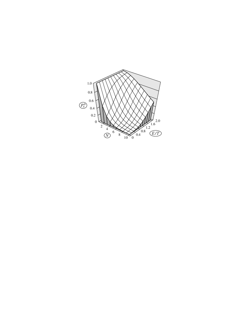
Figure 2: A probability of phase transition without formation of domain walls $P_{N}^{0}$ as function of the number of disconnected subregions $N$ and the ratio of the domain wall energy to the phase transition temperature $E/T$.

The probability of absence of the domain walls becomes on the order of unity (for example, 1/2) if $E/T\geq\ln N$, or, with an account of (5) and (7),

$$\frac{{\mu}^{3}}{\lambda\,T}\>\geq\>\ln\frac{{\eta}_{*}}{{\eta}_{0}}\,.$$ (14)

Because of a very weak logarithmic dependence in the right-hand side of inequality (14), this condition can be satisfied for some particular kinds of the Lagrangians. Therefore, EPR correlations may be an efficient mechanism of the domain wall suppression in a certain class of field theories.

In conclusion, it should be emphasized that the same approach, based on accounting for EPR correlations, can be used to refine a concentration of other Higgs field defects (e.g., magnetic monopoles), which is one of key aspects of the modern astroparticle physics $\!{{\bf??}}$. The refined concentrations, in general, should be less than the commonly accepted ones, and therefore the cosmological constraints on the parameters of the respective field theories will be less tight.

References

References

- [1] N.N.Bogoliubov, Suppl. Nuovo Cimento (Ser. prima) 4, 346 (1966).
- [2] Ya.B.Zel’dovich, I.Yu.Kobzarev, and L.B.Okun, Zh.Eksp.Teor.Fiz. 67, 3 (1974) [Sov.Phys.—JETP 40, 1 (1975)].
- [3] A.D.Linde, Usp.Fiz.Nauk 144, 177 (1984) [Rep.Prog.Phys. 47, 925 (1984)].
- [4] A.Einstein, B.Podolsky, and N.Rosen, Phys.Rev. 47, 777 (1935).
- [5] A.N.Oraevsky, Usp.Fiz.Nauk 168, 1311 (1998) [Phys.—Usp. 41, 1199 (1998)].
- [6] C.W.Misner, Phys.Rev.Lett. 22, 1071 (1969).
- [7] A.Isihara, “Statistical Physics” (Academic Press, NY), 1971.
- [8] Yu.V.Dumin, in “Hot Points in Astrophysics” (Proceedings of the International Workshop), JINR, Dubna, 114, 2000.
- [9] H.V.Klapdor-Kleingrothaus and K.Zuber, “Particle Astrophysics” (Inst. Phys.Publ., Bristol), 1997.