We analyze the CP problem in the context of a supersymmetric extension of the standard model with universal strength of Yukawa couplings. A salient feature of these models is that the CP phases are constrained to be very small by the hierarchy of the quark masses and the pattern of CKM mixing angles. This leads to a small amount of CP violation from the usual KM mechanism and a significant contribution from supersymmetry is required. Due to the large generation mixing in some of the supersymmetric interactions, the electric dipole moments impose severe constraints on the parameter space, forcing the trilinear couplings to be factorizable in matrix form. We find that the $LL$ mass insertions give the dominant gluino contribution to saturate $\varepsilon_{K}$. The chargino contributions to $\varepsilon^{\prime}/\varepsilon$ are significant and can accommodate the experimental results. In this framework, the standard model gives a negligible contribution to the CP asymmetry in B–meson decay, $a_{J/\psi K_{S}}$. However, due to supersymmetric contributions to $B_{d}-\bar{B}_{d}$ mixing, the recent large value of $a_{J/\psi K_{S}}$ can be accommodated.

1 Introduction

The understanding of the origin of fermion families and the observed pattern of fermion masses and mixings, together with the origin of CP violation, are among the major outstanding problems in particle physics. In the standard model (SM), since the flavour structure of the Yukawa couplings is not defined by the gauge symmetry, fermion masses and mixings are arbitrary parameters, to be fixed by experiment. A salient feature of the pattern of quark masses and mixings is the fact that the spectrum is strongly hierarchical and the mixings are small.

Concerning CP violation, it arises in the SM from complex Yukawa couplings which lead to a physical $\delta_{CKM}$ phase in the Cabibbo-Kobayashi-Maskawa (CKM) matrix. The strength of CP violation in the SM is given by ${\mathrm{Im}}\,|Q_{CP}|$, with $Q_{CP}$ denoting any rephasing invariant quartet of the CKM matrix. If one considers the quartet $Q_{CP}=(V_{us}V_{cb}V_{ub}^{*}V_{cs}^{*})$, the experimental value of the moduli entering in this quartet constrains $|Q_{CP}|$ to be of order $10^{-5}$, while the observed strength of CP violation in the kaon sector requires $\phi\equiv\arg(V_{us}V_{cb}V_{ub}^{*}V_{cs}^{*})$ to be of order one. Although in the SM no explanation is provided for the experimentally observed values of $|V_{ij}|$, once these values are incorporated, the SM accommodates in a natural way the observed strength of CP violation in the kaon sector, measured by the parameter $\varepsilon_{K}$. On the other hand, it has been established [1] that the strength of the CP violation in the SM is not sufficient to generate the observed size of the baryon asymmetry of the Universe. This provides the strongest motivation to consider new sources of CP violation, beyond the one present in the SM.

In supersymmetric (SUSY) extensions of the SM there are additional sources of CP violation, due to the presence of new CP violating phases. However, these new phases are severely constrained by experimental bounds on electric dipole moments (EDMs) [2, 3]. Setting these new phases to zero is not natural in the sense of ’t Hooft [4] since the Lagrangian does not acquire any new symmetry in the limit where these new phases vanish. This is the so-called SUSY CP-problem. Since the question of CP-violation is closely related to the general flavour problem, one may wonder whether it is possible, within a supersymmetric extension of the SM, to establish a connection between the need for small CP violating phases and the observed pattern of quark masses and mixings.

Such a connection is possible if one imposes universality of strength for Yukawa couplings (USY) on a SUSY extension of the SM. The idea of USY consists of assuming that all Yukawa couplings have the same modulus, the flavour dependence being all contained in the phases [5]. This leads to what is known as pure phase mass matrices [6]. This class of couplings can be motivated by local horizontal symmetries (see Appendix), and it has also been recently shown that such textures may naturally arise within the framework of a theory with two ”large” extra dimensions [7].

The fact that the quark masses are strongly hierarchical, together with the smallness of $|V_{cb}|$, $|V_{ub}|$ implies that these phases have to be small, at most of order $m_{2}/m_{3}$ [5, 8]. One is then led to a scenario where the strength of CP violation through the Kobayashi-Maskawa (KM) mechanism is naturally small, in fact too small to account for the observed CP violation (CPV) in the kaon sector. This provides motivation for embedding the USY ansatz in a larger framework, where new sources of CP violation naturally arise.

In this paper, we impose the USY ansatz in the framework of SUSY. This extension is specially interesting since new SUSY contributions to CP violation in the kaon sector may play an important rôle in providing sufficient CP violation to saturate the experimental value of $\varepsilon_{K}$.

We study the question of electric dipole moments (EDMs) in supersymmetric USY models. Although the CP violating phases of the Yukawa couplings are small, the USY ansatz implies a large generation mixing in some of the SUSY interactions, which in turn leads to potentially large contributions to the EDMs. The recent bound from the mercury atom EDM [9] sets important restrictions on the class of models we are considering. We will show that due to these constraints one can only saturate the observed value of $\varepsilon_{K}$ with non-universality of the soft trilinear couplings.

Finally, we analyze CP violation in the B-sector. Both the BaBar [10] and Belle [11] collaborations have provided clear evidence for CP violation in the B–system, although at present the experimental errors are relatively large. The large CP asymmetries observed by BaBar and Belle are in rough agreement with the SM predictions. However, there is still quite a large room for new physics and models with small CP violating phases like USY, as well as some of the models with CP as an approximate symmetry [12] might remain phenomenologically viable, provided there are new physics contributions to $\varepsilon_{K}$, $\varepsilon^{\prime}/\varepsilon$, and $B_{d}-\bar{B}_{d}$ mixing [13].

This paper is organized as follows. In Section 2 we present the main features of the USY ansatz for the Yukawa couplings. We show that USY is preserved under the renormalization group (RG) evolution, and give a specific example of a choice of USY phases that leads to a correct quark mass spectrum and $|V^{\mathrm{CKM}}_{ij}|$. In Section 3 we implement the USY hypothesis within a supersymmetric extension of the standard model and investigate how the EDM constrains the SUSY parameter space. The remaining of the section is devoted to the study of the kaon system CPV observables. In Section 4 we analyze the implications of small CPV phases for CP asymmetries in $B_{d}$ meson decays. Our conclusions are presented in Section 5.

2 Universal strength of Yukawa couplings

In the absence of a fundamental theory of flavour, one is tempted to consider some special pattern for the Yukawa couplings, in the hope that they could naturally arise from a flavour symmetry, imposed at a higher energy scale. As mentioned in the introduction, one of the simplest suggestions for the structure of the Yukawa couplings consists of assuming that they have a universal strength $g_{y}$, so that the mass matrices can be written as $m_{ij}=g_{y}v/\sqrt{2}\exp(i\phi_{ij})$, where $i,j$ denote family indices. In the limit of small phases, the USY matrices can be viewed as a perturbation of the democratic type matrices [14].

Within the USY framework, the quark Yukawa couplings can be parametrised as follows:

$$U_{ij}=\frac{\lambda_{u}}{3}\exp\left[i\Phi^{u}_{ij}\right]\quad\mathrm{and}\quad D_{ij}=\frac{\lambda_{d}}{3}\exp\left[i\Phi^{d}_{ij}\right]\;,$$ (1)

where $\lambda_{u,d}$ are overall real constants, and $\Phi^{u,d}$ are pure phase matrices. By performing appropriate weak-basis (WB) transformations the matrices $U$ and $D$ can, without loss of generality, be put in the form

$$U=\frac{\lambda_{u}}{3}\left(\begin{array}[]{ccc}e^{i{p_{u}}}&e^{i{r_{u}}}&1\\ e^{i{q_{u}}}&1&e^{i{t_{u}}}\\ 1&1&1\end{array}\right)\;;\quad\quad D=\frac{\lambda_{d}}{3}K^{\dagger}\left(\begin{array}[]{ccc}e^{i{p_{d}}}&e^{i{r_{d}}}&1\\ e^{i{q_{d}}}&1&e^{i{t_{d}}}\\ 1&1&1\end{array}\right)K\;,$$ (2)

where $K={\mathrm{diag}}(1,e^{i\kappa_{1}},e^{i\kappa_{2}})$.

The phases $\kappa_{i}$ do not affect the spectrum of quark masses, but influence $V_{\mathrm{CKM}}$. The phases ${(p,q,r,t)}$ affect both the spectrum and $V_{\mathrm{CKM}}$. As previously remarked, the hierarchical character of the quark masses constrains each of these latter phases to be small. In order to see how these constraints arise, it is useful to define the Hermitian matrices $H_{u,d}=3/\lambda_{u,d}^{2}\;QQ^{\dagger}$, where $Q=U,D$. It can then be readily verified that the second invariant of $H$ is given by [5]

$$\chi(H)=\frac{4}{9}\sum_{m}\sin^{2}\sigma_{m}=9\;\frac{m_{1}^{2}m_{2}^{2}+m_{1}^{2}m_{3}^{2}+m_{2}^{2}m_{3}^{2}}{{(m_{1}^{2}+m_{2}^{2}+m_{3}^{2})}^{2}}\;,$$ (3)

where, in each sector, $\sigma_{m}$ are linear combinations of the phases ${(p,q,r,t)}$. Since $\chi(H)$ is a sum of positive definite quantities, the modulus of each of the phases has to be small, at most of order $m_{2}/m_{3}$. As mentioned above, the phases $\kappa_{i}$ do not affect the quark spectrum. However, it has been shown [8] that the fact that ${(|V_{cb}|^{2}+|V_{ub}|^{2})}$ is small, constrains each one of the phases $\kappa_{1},\kappa_{2}$ to be at most of order $|V_{cb}|$. As we will see, these $\kappa$ phases will prove to be essential to control the size of the $V_{\mathrm{CKM}}$ elements, in particular that of $V_{td}$.

In our search for a choice of phases leading to the correct masses and mixings, we expand both $\chi(H)$ and the determinant of $H$ in the limit of small phases, and per each of the quark sectors, we write two of the phases as functions of the masses and of the remaining two phases. At this point, we have still some freedom, which we use to fit the experimental bounds on the $V_{\mathrm{CKM}}$ matrix. Therefore, for fixed values of the quark masses and using as input the phases $p_{u,d}$, $r_{u,d}$ and $\kappa_{i}$, we find regions of the phase-parameter space where one correctly reproduces the masses and mixings of the quarks.

As referred in the introduction, USY can be generated at some high energy scale through the breaking of a flavour symmetry. In Ref. [5], it was shown that USY can account for the quark mass spectrum at low energy scales and thus it is important to investigate whether this structure for the Yukawa couplings is preserved by the renormalization group equations (RGE) [16].

At the weak scale, the phases required to explain the fermion masses and mixings are small, hence we can expand the Yukawa couplings of Eq. (1) as

$$U_{ij}=\frac{\lambda_{u}}{3}\left[E_{ij}+i\Phi^{u}_{ij}\right]\quad\mathrm{and}\quad D_{ij}=\frac{\lambda_{d}}{3}\left[E_{ij}+i\Phi^{d}_{ij}\right]\;.$$ (4)

In the above equation, we neglected terms $\mathcal{O}(\Phi^{2}_{q})$, and $E$ is the democratic matrix, defined as $E_{ij}=1,\;\forall i,j$ . The RGE for the real part of Eq. (4) can be easily identified with the evolution of the top and bottom Yukawa couplings:

$$\frac{d\;\lambda_{u}}{dt}=\frac{1}{16\pi^{2}}\left(-G_{u}+6\lambda_{u}^{2}+\lambda_{d}^{2}\right)\lambda_{u}\;,$$

$$\frac{d\;\lambda_{d}}{dt}=\frac{1}{16\pi^{2}}\left(-G_{d}+6\lambda_{d}^{2}+\lambda_{u}^{2}+\lambda_{l}^{2}\right)\lambda_{d}\;,$$ (5)

where $G_{k}(t)=\sum_{i=1}^{3}c^{i}_{k}\;g^{2}_{i}(t)$, with $g_{i}(t)$ the running gauge couplings for $SU(3)\times SU(2)\times U(1)$ gauge group and $c_{k}$ the MSSM RGE coefficients. The reason why, in this limit, the running of the overall Yukawa coefficient decouples from the running of the phases becomes clear if, by means of a weak basis transformation, one moves from the USY basis to the “heavy” basis $(Y\to Y^{\prime}=F^{\dagger}YF)$, where

$$Y_{u,d}^{\prime}=\frac{\lambda_{u,d}}{3}\left[{\mathrm{diag}}(0,0,3)+i\varphi^{u,d}_{ij}\right]\;,\;\mathrm{with}$$ (6)

$$\varphi^{k}(t)=F^{\dagger}\Phi^{k}F\quad\mathrm{and}\quad F=\left[\begin{array}[]{ccc}1/\sqrt{2}&-1/\sqrt{6}&1/\sqrt{3}\\ 0&2/\sqrt{6}&1/\sqrt{3}\\ -1/\sqrt{2}&-1/\sqrt{6}&1/\sqrt{3}\\ \end{array}\right]\;.$$ (7)

The lighter generation Yukawa couplings are thus small perturbations of the leading third generation, originated by the small USY phases.

The running of the imaginary parts is

$$\frac{d\;\Phi^{u}}{dt} =\frac{1}{16\pi^{2}}\left[\lambda_{u}^{2}(-3I+E)+\frac{\lambda_{d}^{2}}{3}(-3I+E)\right]\Phi^{u}+\frac{1}{16\pi^{2}}\left(\frac{\lambda_{u}^{2}}{3}\Delta^{u}+\frac{\lambda_{d}^{2}}{9}\Delta^{d}\right)E\;,$$

$$\frac{d\;\Phi^{d}}{dt} =\frac{1}{16\pi^{2}}\left[\lambda_{d}^{2}(-3I+E)+\frac{\lambda_{u}^{2}}{3}(-3I+E)\right]\Phi^{d}+\frac{1}{16\pi^{2}}\left(\frac{\lambda_{d}^{2}}{3}\;\Delta^{d}E+\frac{\lambda_{u}^{2}}{9}\Delta^{u}E\right)\;,$$ (8)

where $I$ denotes the $3\times 3$ identity matrix and $\Delta^{k}=\Phi^{k}E-E({\Phi^{k}})^{T}$. The scale dependence of the phases can be explicitly analyzed if we write Eqs. (2) in the “heavy” basis:

$$\frac{d\;\varphi^{u}}{dt}=-(3k_{u}^{2}+k_{d}^{2})\left[\begin{array}[]{ccc}\varphi^{u}_{11}&\varphi^{u}_{12}&0\\ \varphi^{u}_{21}&\varphi^{u}_{22}&0\\ 0&0&0\\ \end{array}\right]-k_{d}^{2}\left[\begin{array}[]{ccc}0&0&\varphi^{u}_{13}-\varphi^{d}_{13}\\ 0&0&\varphi^{u}_{23}-\varphi^{d}_{23}\\ 0&0&0\\ \end{array}\right]\;,$$ (9)

$$\frac{d\;\varphi^{d}}{dt}=-(3k_{d}^{2}+k_{u}^{2})\left[\begin{array}[]{ccc}\varphi^{d}_{11}&\varphi^{d}_{12}&0\\ \varphi^{d}_{21}&\varphi^{d}_{22}&0\\ 0&0&0\\ \end{array}\right]-k_{u}^{2}\left[\begin{array}[]{ccc}0&0&\varphi^{d}_{13}-\varphi^{u}_{13}\\ 0&0&\varphi^{d}_{23}-\varphi^{u}_{23}\\ 0&0&0\\ \end{array}\right]\;,$$ (10)

where we defined $k^{2}_{j}(t)=\lambda_{j}^{2}(t)/16\pi^{2}$.

We have performed the analysis of the scale dependence of the phases in the framework of the SM and in the MSSM. The differential equations were solved numerically and analytically, the latter in the limit of small phases. In both cases we have found that if the USY phases are small at some initial scale (which in a phenomenologically consistent model is justified by the smallness of the phases required to fit the quark masses and the $V_{\mathrm{CKM}}$ at the weak scale), then the approximation of Eq. (4) remains valid to energies up to the GUT scale.

The explicit dependence of the phases on the scale can be easily displayed for the low $\tan\beta$ regime, where one can neglect terms in $\lambda_{d}^{2}$ and $\lambda_{l}^{2}$ relatively to the leading $\lambda_{u}^{2}$ contributions. In this limit, the evolution of the up phases is given by

$$\Phi^{u}(t)=a(t)\Phi^{u}(0)+(1-a(t))\chi^{u}\;,$$ (11)

where $a(t)=\exp\left(-3\int^{t}_{0}k_{u}^{2}(t^{\prime})dt^{\prime}\right)$ contains the scale dependence and

$$\chi^{u}=F\left[\begin{array}[]{ccc}0&0&\varphi^{u}_{13}(0)\\ 0&0&\varphi^{u}_{23}(0)\\ \varphi^{u}_{31}(0)&\varphi^{u}_{32}(0)&\varphi^{u}_{33}(0)\\ \end{array}\right]F^{\dagger}\;,$$ (12)

is a function of the initial phases; the structure of $\chi^{u}$ allows these to be combined so that the up quark Yukawa coupling for low $\tan\beta$ values takes the form:

$$U(t)=\frac{\lambda_{u}(t)}{3}\;{K_{L}^{u}}^{\dagger}\;e^{ia(t)\Phi^{u}(0)}\;K_{R}^{u}\;,$$ (13)

where $K_{L}^{u}$ and $K_{R}^{u}$ are diagonal phase matrices, whose entries depend on the initial phases contained in the matrix $\chi^{u}$ and on the integral $a(t)$.

The analysis for the down sector is entirely analogous. In the low $\tan\beta$ regime, the solution for the running of the down phases takes the form:

$$\Phi^{d}(t)=b(t)\Phi^{d}(0)+(1-b(t))\chi^{d}+d(t)\eta^{u}\;,$$ (14)

where $b(t)=\exp\left(-\int^{t}_{0}k_{u}^{2}(t^{\prime})dt^{\prime}\right)$ and $d(t)=-b(t)\int^{t}_{0}\frac{k_{u}^{2}(t^{\prime})}{b(t^{\prime})}dt^{\prime}$. The matrices $\chi^{d}$ and $\eta^{u}$ are also functions of the initial phases.

$$\chi^{d}=F\left[\begin{array}[]{ccc}0&0&0\\ 0&0&0\\ \varphi^{d}_{31}(0)&\varphi^{d}_{32}(0)&\varphi^{d}_{33}(0)\\ \end{array}\right]F^{\dagger}\;,\quad\eta^{u}=F\left[\begin{array}[]{ccc}0&0&\varphi^{u}_{13}(0)\\ 0&0&\varphi^{u}_{23}(0)\\ 0&0&0\\ \end{array}\right]F^{\dagger}\;.$$ (15)

Just like in the previous case, these phase matrices can be reorganised so that the down Yukawa coupling evolution reads:

$$D(t)=\frac{\lambda_{d}(t)}{3}{K_{L}^{d}}^{\dagger}\;Q\;e^{ib(t)\Phi^{d}(0)}\;K_{R}^{d}\;,$$ (16)

where $K_{L}^{d},\ K_{R}^{d}$ and $Q$ are diagonal phase matrices; the first two depend on the function $b(t)$ and on the phases appearing on $\chi^{d}$, while the third depends on $d(t)$ and $\eta^{u}$.

By means of yet another weak basis transformation, one can still rewrite the Yukawa couplings in Eqs. (13,16) as

$$U(t)\;\rightarrow\;\frac{\lambda_{u}(t)}{3}\;e^{ia(t)\Phi^{u}(0)}\;;\quad\quad D(t)\;\rightarrow\;\frac{\lambda_{d}(t)}{3}\;P^{\dagger}\;e^{ib(t)\Phi^{d}(0)}\;P\quad\quad(P=Q^{\dagger}K^{d}_{L}{K^{u}_{L}}^{\dagger})\;.$$ (17)

This means that it is always possible to move to a basis where the Yukawa couplings are easily related to the original ones. Obviously, the $P$ matrices have no effect on the quark spectrum, only on $V_{\mathrm{CKM}}$. Therefore RG evolution preserves the USY texture that is responsible for the non-degenerate quark spectrum. For the case of large $\tan\beta$, the argument can be equally verified.

At this point, one should make a final remark regarding the possibility of having Hermitian and USY Yukawa couplings, that is having the phase matrices verify the condition $\Phi^{q}_{ij}=-\Phi^{q}_{ji}$, ($q=u,d$). As it was first pointed out in [17], Hermitian USY leads to a sum rule for the quark masses, namely $m_{1}\;m_{2}+m_{2}\;m_{3}+m_{1}\;m_{3}=0$, which is clearly violated by experiment. The question that naturally follows is whether Hermitian USY textures imposed at some higher energy (GUT scale, for example) can produce a phenomenologically viable texture through RG effects. As it can be seen from Eqs. (13,16, 17), if one starts with Hermitian structures, that is $\Phi^{q}_{ij}(0)=-\Phi^{q}_{ji}(0)$, we find that at any other scale one can always rotate to a basis where the phases that govern the spectrum scale with the flavour-independent coefficients $a(t)$ and $b(t)$, so that the impossibility of having Hermitian USY textures holds at any scale.

To illustrate some of the features of this ansatz, let us consider, as an example, the following choice of USY phases:

$$U = \frac{\lambda_{u}}{3}\left(\begin{array}[]{ccc}e^{i\;0.000517}&e^{-i\;0.0000074}&1\\ e^{-i\;0.01438}&1&e^{i\;0.00158}\\ 1&1&1\end{array}\right),\;$$ (21)

$$D = \frac{\lambda_{d}}{3}K^{\dagger}\left(\begin{array}[]{ccc}e^{i\;0.00229}&e^{i\;0.02833}&1\\ e^{-i\;0.09278}&1&e^{-i\;0.1453}\\ 1&1&1\end{array}\right)K\;,$$ (25)

$$K = {\mathrm{diag}}(1\;,\;1\;,\;e^{i\;0.0138})\;.$$ (26)

The overall factor has been defined as $\lambda_{u}/3=m_{t}/v\sin\beta$ and $\lambda_{d}/3=m_{b}/v\cos\beta$.

The Yukawa couplings can be diagonalized by means of the transformations

$$S_{R}^{d(u)}~{}Y^{d(u)^{T}}~{}S_{L}^{d(u)^{{\dagger}}}=Y^{d(u)}_{\mathrm{diag}}\;,$$ (27)

where $S_{R}$ and $S_{L}$ are unitary matrices. In the present USY model we find

$$S_{L}^{u}=\left(\begin{array}[]{ccc}0.695&0.0236-1.66\times 10^{-4}\;i&-0.719+1.83\times 10^{-4}\;i\\ -0.429&0.816-3.72\times 10^{-3}\;i&-0.388+1.65\times 10^{-4}\;i\\ 0.577i&2.56\times 10^{-3}+0.577\;i&9.79\times 10^{-5}+0.577\;i\end{array}\right)\;,$$ (28)

$$S_{L}^{d}=\left(\begin{array}[]{ccc}0.772&-0.157+0.0122\;i&-0.615-4.99\times 10^{-4}\;i\\ -0.264&0.798-0.0759\;i&-0.537+3.05\times 10^{-3}\;i\\ 0.578\;i&0.511+0.575\;i&-2.07\times 10^{-3}+0.577\;i\end{array}\right)\;,$$ (29)

and the associated $V_{\mathrm{CKM}}$

$$V_{\mathrm{CKM}}=\left(\begin{array}[]{ccc}0.975-6.88\times 10^{-4}\;i&0.221+3.96\times 10^{-3}\;i&0.0027-4\times 10^{-5}\;i\\ -0.220-9.71\times 10^{-3}\;i&0.973+0.061\;i&0.041+1.92\times 10^{-3}\;i\\ 0.0063+1.10\times 10^{-4}\;i&-0.041-1.75\times 10^{-3}\;i&0.999+0.027\;i\end{array}\right)\;.$$ (30)

Within the context of the SM, the matrices $S_{L,R}^{u,d}$ do not have, by themselves, any physical meaning, only the combination $S_{L}^{u}.{S_{L}^{d^{\dagger}}}\equiv V_{\mathrm{CKM}}$ is physically meaningful. However the matrices $S_{L,R}^{u,d}$ do play a significant rôle in some extensions of the SM, as, for example the MSSM with non–universal soft-breaking terms. We shall discuss this question in the following sections.

The values of the moduli of the above presented $V_{\mathrm{CKM}}$ are in agreement with the experimental bounds. The central value of $|V_{td}|$ ($|V_{td}|\sim 0.0063$) is somewhat smaller than the central value of $|V_{td}|$ extracted from experiment [18], within the context of the SM, namely $|V_{td}|=0.0073$. However, it should be noted that in the framework of the SM, the value of $|V_{td}|$ is derived from the experimental value of $B_{d}-\bar{B}_{d}$ mixing, and not from tree-level decays, as it is the case for the moduli of the first two rows of $V_{\mathrm{CKM}}$. Since in the SM, $B_{d}-\bar{B}_{d}$ mixing only receives contributions at one loop level, there may be non-negligible contributions to $B_{d}-\bar{B}_{d}$ mixing from physics beyond the SM.

Concerning CP violation, it can be readily verified that the above $V_{\mathrm{CKM}}$ leads to a strength of CP breaking (measured by $J\equiv{\mathrm{Im}}\,(V_{ud}V_{cs}V^{*}_{us}V^{*}_{cd})$ [19]) that is too small to account for the observed value of $\varepsilon_{K}$. In fact, for the above example, one obtains $J\sim 10^{-7}$, which is to be compared to the required value of $J\sim 10^{-5}$. This is a generic feature of the USY ansatz. Although one can obtain somewhat larger values of $J$ (e.g. $J\sim 10^{-6}$) for a different choice of USY phases [5], the tendency in this class of ansätze is to have values of $J$ which are too small to saturate the experimental value of $\varepsilon_{K}$. This motivates the embedding of USY in a larger framework where new sources of CP violation naturally arise. In the following sections we address this question in the context of supersymmetric extensions of the standard model.

3 Supersymmetric USY models and CP violation

As advocated in the introduction, supersymmetric extensions of the SM may provide a considerable enhancement to CP violation observables, since in addition to containing new “genuine” CPV phases, they introduce new flavour structures. Accordingly, SUSY emerges as the natural candidate to solve the problem of CP violation inherent to the USY models discussed in the previous section. We recall that within the USY framework the amount of CP violation arising from the CKM mechanism is typically quite small, hence one will need significant supersymmetric contributions that both succeed in saturating the values of the CP violating observables and in having EDM contributions which do not violate the current experimental bounds.

We will consider the minimal supersymmetric standard model (MSSM), where a minimal number of superfields is introduced and $R$ parity is conserved, with the following soft SUSY breaking terms

$$V_{SB} = m_{0\alpha}^{2}\phi_{\alpha}^{*}\phi_{\alpha}+\epsilon_{ab}(A^{u}_{ij}Y^{u}_{ij}H_{2}^{b}\tilde{q}_{L_{i}}^{a}\tilde{u}^{*}_{R_{j}}+A^{d}_{ij}Y^{d}_{ij}H_{1}^{a}\tilde{q}_{L_{i}}^{b}\tilde{d}^{*}_{R_{j}}+A^{l}_{ij}Y^{l}_{ij}H_{1}^{a}\tilde{l}_{L_{i}}^{b}\tilde{e}^{*}_{R_{j}}$$ (31)

$$- B\mu H_{1}^{a}H_{2}^{b}+\mathrm{H.c.})-\frac{1}{2}(m_{3}\bar{\tilde{g}}\tilde{g}+m_{2}\overline{\widetilde{W^{a}}}\widetilde{W}^{a}+m_{1}\bar{\tilde{B}}\tilde{B})\;,$$

where $i,j$ are family indices, $a,b$ are $SU(2)$ indices, and $\epsilon_{ab}$ is the $2\times 2$ fully antisymmetric tensor, with $\epsilon_{12}=1$. Moreover, $\phi_{\alpha}$ denotes all the scalar fields of the theory. Although in general the parameters $\mu$, $B$, $A^{\alpha}$ and $m_{i}$ can be complex, two of their phases can be rotated away [21]. In a minimal SUGRA scenario (mSUGRA), the soft SUSY breaking parameters are universal at some very high energy scale (which we take to be the GUT scale), and we can write

$$m_{0\alpha}^{2}=m_{0}^{2}\;,\quad m_{i}=m_{1/2}\;,\quad A^{\alpha}_{ij}=A_{0}e^{i\phi_{A}}\;.$$ (32)

In this case, there are only two physical phases

$$\phi_{A}=\arg(A^{*}m_{1/2}),~{}~{}~{}\phi_{\mu}=\arg(\mu~{}m_{1/2}).$$ (33)

In order to have EDM values below the experimental bounds, and without forcing the SUSY masses to be unnaturally heavy, the phases $\phi_{A}$ and $\phi_{\mu}$ must be at most of order $10^{-2}$ [2]. Thus, in this class of SUSY models with minimal flavour violation, complex Yukawa couplings leading to a physical $\delta_{CKM}$ phase in the CKM matrix are the main source of CP violation. It should be also stressed that even if one ignores the bounds from the EDMs, and allows $\phi_{A}$ and $\phi_{\mu}$ to be of order one, the latter models do not generate any sizeable new contribution to $\varepsilon_{K}$ and $\varepsilon^{\prime}/\varepsilon$ [22] apart from those present in the SM. In the mSUGRA scenario of Eq.(32), the USY structure of the Yukawa couplings is inherited by the trilinear terms so this simple flavour structure is excluded, since, and as aforementioned, no new contributions to CPV observables are generated. However, in general supergravity scenarios [23], the Yukawa couplings can be independent of the hidden sector fields that break supersymmetry and hence one can have $A$-terms with a flavour structure that is not related to that of the Yukawa couplings. This has recently motivated a growing interest on supersymmetric models with non–universal soft breaking terms, and a considerable amount of work has been devoted to the analysis of the effects of the new flavour textures on the CPV observables [24, 25, 26].

Regarding the non–universality of the trilinear soft terms, it has been emphasized that a new flavour structure in the $A$ terms can saturate the experimental bounds on $\varepsilon_{K}$ and $\varepsilon^{\prime}/\varepsilon$ even in the presence of a vanishing $\delta_{CKM}$ [24, 25]. However, the phases associated with the $A$–term diagonal elements might induce large EDMs. The latter problem can be overcome if one takes the Yukawa couplings and the $A$–terms to be Hermitian, in order to ensure that the diagonal elements of $A_{ij}Y_{ij}$ are real in any basis [26, 27]. This problem is also less severe if the trilinear terms can be factorized as $A_{ij}Y_{ij}=A.Y$ or $Y.A$, an interesting possibility that naturally arises withing the context of general SUGRA models [25]. As we will discuss below, this factorization implies that the mass insertion $(\delta_{11}^{d})_{LR}$ (which is the most relevant to the EDMs contributions) is suppressed by the ratio $m_{d}/m_{\tilde{q}}$, where $m_{d}$ is the down quark mass and $m_{\tilde{q}}$ is an average squark mass.

The non-universality of the squark mass matrices, which can be arbitrary in generic SUSY models, is not constrained by the EDMs. Nevertheless, $\Delta m_{K}$ and $\varepsilon_{K}$ impose severe constraints on the squark mixing, which can still be avoided in models with flavour symmetries or squark-quark alignment [28].

After this brief discussion, we begin the analysis of the implications of having USY Yukawa couplings within a supersymmetric scenario of CP violation. As in most SUSY models, the trilinear terms will play a key rôle, since they are directly related with the increasingly more stringent bounds coming from the EDMs. In what follows, we will study the enhancement of the CP observables through the non-universalities of the soft breaking terms in supersymmetric USY models.

3.1 Constraints from the electric dipole moments

In this section we investigate how the EDM bounds constrain the parameter space for SUSY models with universal strength of Yukawa couplings. The current experimental bound on the EDM of the neutron is given by  [29]

$$d_{n}<6.3\times 10^{-26}\;e\ \mathrm{cm}\quad(90\%~{}\mathrm{C.L.}).$$ (34)

This bound can be translated into constraints for the imaginary parts of the flavour conserving $LR$ mass insertions.

$$(\delta_{11}^{d(u)})_{LR}=\frac{1}{\tilde{m}_{q}^{2}}\left[\left(S_{L}^{d(u)}~{}Y^{A^{*}}_{d(u)}~{}S_{R}^{d(u)^{{\dagger}}}\right)_{11}v_{1(2)}-\mu Y_{1}^{d(u)}~{}v_{2(1)}\right],$$ (35)

where $\tilde{m}_{q}^{2}$ is the average squark mass and $v_{i}=\left\langle H^{0}_{i}\right\rangle/\sqrt{2}$. In our analysis, the $\mu$ term is assumed to be real and its magnitude is computed from electroweak symmetry breaking. Recall that $S_{L}^{d(u)}$ and $S_{R}^{d(u)}$ are the rotation matrices that diagonalize the down (up) Yukawa couplings. For the specific case of USY couplings discussed in Section 2, the structure of $S_{L}^{d(u)}$ was presented in Eqs. (28,29). $S_{R}^{d(u)}$ manifest the same large intergenerational mixing and large phases. The effects of these phases are absent in the SM and in supersymmetric models with universal soft-breaking terms (i.e., flavour structures that are aligned with the Yukawa couplings). Nevertheless, the effect of any minimal deviation from this scenario, particularly regarding the non-degeneracy of the trilinear terms, is strongly enhanced due to the large mixing, providing significant contributions to CP violation observables. On the other hand, the bounds arising from the experimental measurements of the EDMs severely constrain any non-degeneracy of the trilinear terms, even in the limit of vanishing SUSY phases. Imposing that $d_{n}$ does not exceed the experimental limit requires ${\mathrm{Im}}\,(\delta^{d(u)}_{11})_{LR}$ to be less than $10^{-6}$. However, a stronger constraint on these mass insertions comes from the recently measured electric dipole moment of the mercury atom [9]

$$d_{Hg}<2.1\times 10^{-28}\;e\ \mathrm{cm}\;.$$ (36)

This constraint corresponds to having $\mathrm{Im}(\delta^{d(u)}_{11})_{LR}\raise 1.29167pt\hbox{$\;<$\kern-7.5pt\raise-4.73611pt\hbox{$\sim\;$}}10^{-7}-10^{-8}$. Since the mercury EDM also receives considerable contributions from strange quarks, one has in addition $\mathrm{Im}(\delta^{d}_{22})_{LR}\raise 1.29167pt\hbox{$\;<$\kern-7.5pt\raise-4.73611pt\hbox{$\sim\;$}}10^{-5}-10^{-6}$ [2]. These bounds impose a stringent constraint on most supersymmetric models, implying that the CP violating phases are very small and (or) that SUSY soft breaking terms must have a special flavour structure.

Small CP phases can be motivated by an approximate CP symmetry and as previously pointed out, USY provides a natural scenario where all Yukawa coupling phases are bound to be $\raise 1.29167pt\hbox{$\;<$\kern-7.5pt\raise-4.73611pt\hbox{$\sim\;$}}10^{-1}$. In this work we take as a guideline the assumption that all supersymmetric phases should be no greater than the largest of the phases present in the Yukawa textures of Eqs. (21).

Although in many models the trilinear terms do not have the same structure of the Yukawa couplings, when introducing the USY ansatz in a supersymmetric framework the most appealing scenario would be to have a USY texture in the $A$-terms as well. Nevertheless, we have verified that such textures for the $A$-terms do not suceed in providing sizable SUSY contributions to the CPV observables without violating the EDM bounds. Therefore we consider a more general scenario for the trilinear terms, and allow for non-universalities in the magnitude of the several elements. We will show that, even in the limit of small (or vanishing) supersymmetric phases, the large mixing inherent to USY couplings (displayed in $S_{L}$ and $S_{R}$), together with the experimental limits on EDMs, severely constrain any non–universality of the trilinear terms. In Fig. 1 we present the constraints from the EDMs on the off–diagonal entries of the $A$-terms, in particular $A_{12}$ and $A_{13}$. In our analysis we assumed $\tan\beta=5$, $m_{0}=m_{1/2}=250\;{\mathrm{GeV}}$ and $A_{ij}=m_{0}$ for all elements except $A_{12,13}$, which we set in the range $[-3m_{0},3m_{0}]$.

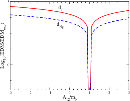
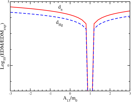
Figure 1: Neutron and mercury EDMs as function of the off–diagonal entries $A_{12}$ and $A_{13}$ for $\tan\beta=5$ and $m_{0}=m_{1/2}=250$ GeV. $A_{ij}=1\;\forall ij\neq 12(13)$ on the left (right) figure.

From these figures, it is clear that any significant non–universality among the $A$ terms (e.g. at $10\%$) leads to unacceptably large EDMs. Similar constraints hold for the other off–diagonal elements $A_{21}$, $A_{31}$, $A_{23}$ and $A_{32}$. It is also worth noticing that such constraints are far more severe than those obtained in the case of hierarchical Yukawa couplings, as a consequence of the already mentioned large intergenerational mixing.

As recently shown, this problem can be overcome if one takes the Yukawa couplings and the $A$–terms to be Hermitian, in order to ensure that the diagonal elements of $A_{ij}Y_{ij}$ are real in any basis [26]. Another interesting possibility is to have trilinear terms that can be factorized as $\hat{A}=A_{ij}Y_{ij}=A.Y$ or $Y.A$  [25]. As above referred, this factorization implies that the mass insertion $(\delta_{11}^{d})_{LR}$ is suppressed by the ratio $m_{d}/m_{\tilde{q}}$.

As an example for the trilinear couplings that avoids the EDM constraints and implies signficant SUSY CP violation, we consider the following structure:

$$A=m_{0}\left(\begin{array}[]{ccc}a&a&a\\ b&b&b\\ c&c&c\end{array}\right)\;.$$ (37)

In this case the trilinear couplings $\hat{A}$ can be written as

$$\hat{A}=\mathrm{diag}(a,b,c)\cdot Y\;.$$ (38)

With this structure for the trilinear couplings, the EDMs do not impose any constraint on the parameters $a,b$, $c$ if these are real, and the associated EDM values are similar to those obtained with universal and real $A$ terms. For complex $a,b$, and $c$, the constraints on the phases $\varphi_{a}$, $\varphi_{b}$, and $\varphi_{c}$ are shown in Fig. 2.

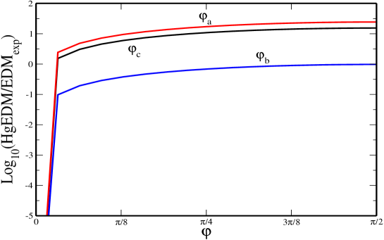
Figure 2: The mercury EDM as function of the trilinear SUSY phases $\varphi$ for $\tan\beta=5$, $m_{0}=m_{1/2}=250$ GeV. $|A_{ij}|=1\;\forall ij$.

As it can be observed for the case of universal $|A_{ij}|$, compatibility with experiment requires

$$\varphi_{a}\raise 1.29167pt\hbox{$\;<$\kern-7.5pt\raise-4.73611pt\hbox{$\sim\;$}}0.05\;\mathrm{rad}\quad\;\quad\quad\varphi_{b}\raise 1.29167pt\hbox{$\;<$\kern-7.5pt\raise-4.73611pt\hbox{$\sim\;$}}\pi/2\;\quad\;;\quad\quad\varphi_{c}\raise 1.29167pt\hbox{$\;<$\kern-7.5pt\raise-4.73611pt\hbox{$\sim\;$}}0.07\;\mathrm{rad}\;.$$ (39)

The reason why the phase $\varphi_{b}$ is much less constrained than $\varphi_{a}$ and $\varphi_{c}$ is that the mixing between the first and the second generations, as observed from Eqs. (28,29), is smaller than the mixing between the first and the third generations. For $|A_{ij}|\simeq 3m_{0}$, the EDMs constraint on these phases becomes more stringent:

$$\varphi_{a}\raise 1.29167pt\hbox{$\;<$\kern-7.5pt\raise-4.73611pt\hbox{$\sim\;$}}0.02\;\mathrm{rad}\quad\;,\quad\quad\varphi_{b}\raise 1.29167pt\hbox{$\;<$\kern-7.5pt\raise-4.73611pt\hbox{$\sim\;$}}0.35\;\mathrm{rad}\quad\;,\quad\quad\varphi_{c}\raise 1.29167pt\hbox{$\;<$\kern-7.5pt\raise-4.73611pt\hbox{$\sim\;$}}0.02\;\mathrm{rad}\;.$$ (40)

Thus, we can conclude that in USY models the maximal allowed non-universality for the $A$-terms is the structure presented in Eq. (37), with the associated SUSY phases ($\varphi_{ij}$) within the limits given in Eq. (40). In view of this, we analyze the contributions to the kaon system CPV observables, $\varepsilon_{K}$ and $\varepsilon^{\prime}/\varepsilon$.

3.2 SUSY contributions to $\varepsilon_{K}$ and $\varepsilon^{\prime}/\varepsilon$

We proceed to investigate how CP violation can further constrain the parameter space for the case of supersymmetric USY models. In the kaon system, the most relevant observables are $\varepsilon_{K}$ and $\varepsilon^{\prime}/\varepsilon$. We first turn our attention to the indirect CP violation parameter, $\varepsilon_{K}$, which is given by

$$\varepsilon_{K}=\frac{e^{i\pi/4}}{\sqrt{2}\Delta m_{K}}{\mathrm{Im}}\,M_{12}\;,$$ (41)

where $M_{12}$ is the off-diagonal entry in the kaon mass matrix and $\Delta m_{K}$ is the mass difference of the short and long-lived kaon states. The kaon mass matrix element can be defined as follows

$$2m_{K}M_{12}^{*}=\left\langle\bar{K}^{0}|\mathcal{H}_{\mathrm{eff}}^{\Delta S=2}|K^{0}\right\rangle\;,$$ (42)

where $\mathcal{H}^{\Delta S=2}_{eff}$ is the effective Hamiltonian (EH) for $\Delta S=2$ transitions, which can be expressed in the operator product expansion as

$$\mathcal{H}^{\Delta S=2}_{eff}=\sum_{i}C_{i}(\mu)Q_{i}\;.$$ (43)

In the above formula, $C_{i}(\mu)$ are the Wilson coefficients and $Q_{i}$ are the EH local operators.
The relevant operators for the gluino contribution are [30]

$$Q_{1} = \bar{d}^{\alpha}_{L}\gamma_{\mu}s^{\alpha}_{L}\bar{d}^{\beta}_{L}\gamma^{\mu}s^{\beta}_{L},~{}~{}~{}~{}~{}~{}Q_{2}=\bar{d}^{\alpha}_{R}s^{\alpha}_{L}\bar{d}^{\beta}_{R}s^{\beta}_{L},~{}~{}~{}~{}~{}~{}~{}Q_{3}=\bar{d}^{\alpha}_{R}s^{\beta}_{L}\bar{d}^{\beta}_{R}s^{\alpha}_{L},$$

$$Q_{4} = \bar{d}^{\alpha}_{R}s^{\alpha}_{L}\bar{d}^{\beta}_{L}s^{\beta}_{R},~{}~{}~{}~{}~{}~{}~{}~{}~{}~{}~{}~{}Q_{5}=\bar{d}^{\alpha}_{R}s^{\beta}_{L}\bar{d}^{\beta}_{L}s^{\alpha}_{R},$$ (44)

as well as the operators $\tilde{Q}_{1,2,3}$, that are obtained from $Q_{1,2,3}$ by the exchange $L\leftrightarrow R$. In the latter equations, $\alpha$ and $\beta$ are $SU(3)_{c}$ colour indices, and the colour matrices obey the normalization ${\mathrm{Tr}}\,(t^{a}t^{b})=\delta^{ab}/2$. Due to the gaugino dominance in the chargino–squark loop, the most significant $\tilde{\chi}^{\pm}$ contribution is associated with the operator $Q_{1}$ [31].

In the presence of supersymmetric ($\tilde{g}$ and $\tilde{\chi}^{\pm}$) contributions, the following result for the amplitude $M_{12}$ is obtained:

$$M_{12}=M_{12}^{\mathrm{SM}}+M_{12}^{\tilde{g}}+M_{12}^{\tilde{\chi}^{\pm}}\;.$$ (45)

The SM contribution can be written as [32, 33]

$$M_{12}^{\mathrm{SM}}=\frac{G_{F}^{2}m^{2}_{W}}{12\pi^{2}}f^{2}_{K}m_{K}\hat{B}_{K}\mathcal{F}^{*}\;,$$ (46)

where $f_{K}$ is kaon decay constant, $\hat{B}_{K}$ is the bag parameter, and the function $\mathcal{F}$ can be found in  [33]. For the specific USY ansatz we are considering, we find that the SM contribution to $\varepsilon_{K}$ is $\mathcal{O}(10^{-5})$. The supersymmetric term $M_{12}^{\tilde{g}}$ is given by

$$M_{12}^{\tilde{g}} = \frac{-\alpha_{S}}{216m_{\tilde{q}^{2}}}\frac{1}{3}m_{K}f_{K}^{2}\Biggl{\{}\left((\delta^{d}_{12})^{2}_{LL}+(\delta^{d}_{12})^{2}_{RR}\right)B_{1}(\mu)\left(24\,x\,f_{6}(x)+66\,\tilde{f}_{6}(x)\right)$$ (47)

$$+ (\delta^{d}_{12})_{LL}(\delta^{d}_{12})_{RR}\left(\frac{m_{K}}{m_{s}(\mu)+m_{d}(\mu)}\right)^{2}\biggl{[}B_{4}(\mu)\left(378\,x\,f_{6}(x)-54\tilde{f}_{6}(x)\right)$$

$$+ B_{5}(\mu)\left(6\,x\,f_{6}(x)+30\tilde{f}_{6}(x)\right)\biggr{]}+\left((\delta^{d}_{12})^{2}_{LR}+(\delta^{d}_{12})^{2}_{RL}\right)\left(\frac{m_{K}}{m_{s}(\mu)+m_{d}(\mu)}\right)^{2}$$

$$\left(-\frac{255}{2}B_{2}(\mu)-\frac{9}{2}B_{3}(\mu)\right)x\,f_{6}(x)+(\delta^{d}_{12})_{LR}(\delta^{d}_{12})_{RL}\left(\frac{m_{K}}{m_{s}(\mu)+m_{d}(\mu)}\right)^{2}$$

$$\biggl{[}-99B_{4}(\mu)-45B_{5}(\mu)\biggr{]}\tilde{f}_{6}(x)\Biggr{\}},$$

where $x=(m_{\tilde{g}}/m_{\tilde{q}})^{2}$ and the functions $f_{6}(x),\tilde{f}_{6}(x)$ are given in Ref.[30]. We have used the matrix elements of the normalized operators $Q_{i}(\mu)$ with the following $B$-parameters at $\mu=2{\mathrm{GeV}}$ [30]

$$B_{1}(\mu) = 0.60\;,~{}~{}~{}~{}~{}~{}~{}~{}~{}~{}B_{2}(\mu)=0.66\;,~{}~{}~{}~{}~{}~{}~{}~{}~{}~{}B_{3}(\mu)=1.05\;,$$

$$B_{4}(\mu) = 1.03\;,~{}~{}~{}~{}~{}~{}~{}~{}~{}~{}B_{5}(\mu)=0.73\;.$$

Finally $M_{12}^{\tilde{\chi}^{\pm}}$ is [31]

$$M_{12}^{\tilde{\chi}^{\pm}}=\frac{g^{2}}{768\pi^{2}m_{\tilde{q}^{2}}}\frac{1}{3}m_{K}f_{K}^{2}B_{1}(\mu)\left(\sum_{a,b}K_{a2}^{*}(\delta^{u}_{LL})_{ab}K_{b1}\right)^{2}\sum_{i,j}|V_{i1}|^{2}|V_{j1}|^{2}H(x_{i},x_{j}),$$ (48)

where $x_{i}=(m_{\tilde{\chi}_{i}^{+}}/m_{\tilde{q}})^{2}$. Here $K$ is the CKM matrix, $a,b$ are flavour indices, $i,j$ label the chargino mass eigenstates, and $V$ is one of the matrices used for diagonalizing the chargino mass matrix. The loop function $H(x_{i},x_{j})$ is given in Ref.[31].

To saturate $\varepsilon_{K}$ from gluino contributions, one should have [34]

$$\sqrt{|\mathrm{Im}(\delta_{12}^{d})_{LL}^{2}|}\sim 10^{-3}\quad\mathrm{or}\quad\sqrt{|\mathrm{Im}(\delta_{12}^{d})_{LR}^{2}|}\sim 10^{-4}\;,$$ (49)

whilst the chargino contributions require

$$\mathrm{Im}(\delta_{12}^{u})_{LL}^{2}\sim 10^{-1}\;.$$ (50)

In the present scenario, using the USY texture of Eq. (21) and $A$-terms as in Eq. (37), we find the correlation between these two mass insertions is as given in Fig. 3.

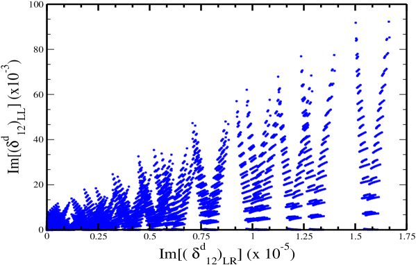
Figure 3: Correlation between $(\delta_{12}^{d})_{LL}$ and $(\delta_{12}^{d})_{LR}$ mass inserions for for $\tan\beta=5$, $m_{0}=m_{1/2}=250$ GeV. $a,b,c$ vary from $[-3,3]$ and $\varphi_{a,b,c}$ are chosen so that the EDMs are consistent with the experimental limits.

From Figure 3, one can see that the $LL$ mass insertions give the dominant gluino contribution to saturate $\varepsilon_{K}$, contrary to the $LR$ mass insertions, which are typically much smaller than the required value given in Eq. (49). In addition, we also find (for $m_{0}=m_{1/2}=250\;{\mathrm{GeV}}$) that $\mathrm{Im}(\delta^{u}_{12})_{LL}\simeq 10^{-3}$, two orders of magnitude below the required value, so that one has a negligible chargino contribution to $\varepsilon_{K}$. Therefore, with USY Yukawa couplings, the MSSM with non–universal $A$-terms (as those given in Eq. (37)) can account for the experimentally observed indirect CP violation in the kaon system.

It is important to note that the behaviour of the $LL$ mass insertion (particularly the significant dependence on the non–universality of the $A$–terms) is in clear contrast with the case of standard hierarchical Yukawa couplings. It is well known that in these scenarios, and with universal scalar soft masses, $\mathrm{Im}(\delta^{d}_{12})_{LL}$ is typically of order $10^{-5}$ and the $LL$ mass insertions are independent of the $A$–terms. In our model, the large mixing displayed by the rotation matrices enhances any non-diagonal contribution to $M^{2}_{\tilde{Q}_{L}}$ induced by the trilinear terms from RG evolution, hence $LL$ mass insertions can account for the experimental value of $\varepsilon_{K}$.

Next we consider SUSY contributions to $\varepsilon^{\prime}/\varepsilon$. The grand average of the experimental values is [35, 36],

$${\mathrm{Re}}\,(\varepsilon^{\prime}/\varepsilon)=(19.2\pm 2.4)\times 10^{-4}\;.$$ (51)

$\varepsilon^{\prime}$ can be given as ratio of isospin amplitudes $A_{I}$, which are defined as

$$A_{I}e^{i\delta_{i}}=\langle\pi\pi(I)|\mathcal{H}_{eff}^{\Delta S=1}|K^{0}\rangle\;,$$ (52)

where $I=0,2$ is the isospin of the final two-pion state. Therefore we can write [33]

$$\frac{\varepsilon^{\prime}}{\varepsilon}\sim\frac{i}{\sqrt{2}}\;e^{i(\delta_{2}-\delta_{0})}\;\frac{{\mathrm{Im}}\,(A_{2}A_{0}^{*})}{{|\varepsilon A_{0}|}^{2}}\;.$$ (53)

Assuming that the strong phase difference ($\delta_{2}-\delta_{0}$) is close to $\pi/4$, the expression for $\varepsilon^{\prime}$ can be rewritten as

$$\frac{\varepsilon^{\prime}}{\varepsilon}=e^{i\frac{\pi}{4}}\frac{\omega}{\sqrt{2}|\varepsilon|}\xi(\Omega-1)$$ (54)

with

$$\omega=\mathrm{Re}A_{2}/\mathrm{Re}A_{0}\;,\quad\xi=\frac{{\mathrm{Im}}\,A_{0}}{{\mathrm{Re}}\,A_{0}}\quad\mathrm{and}\quad\Omega=\frac{{\mathrm{Im}}\,A_{2}}{\omega{\mathrm{Im}}\,A_{0}}\;.$$ (55)

The real parts of both amplitudes are experimentally known to be ${\mathrm{Re}}\,A_{2}=1.5\times 10^{-8}\;{\mathrm{GeV}}$ and ${\mathrm{Re}}\,A_{0}=33.3\times 10^{-8}\;{\mathrm{GeV}}$.

The effective Hamiltonian for $\Delta S=1$ transitions receives contributions from operators with dimension four, five and six, and can be symbolically written as

$$\mathcal{H}_{\mathrm{eff}}^{\Delta S=1}=\mathcal{H}_{\mathrm{eff}}^{(4)}+\mathcal{H}_{\mathrm{eff}}^{(5)}+\mathcal{H}_{\mathrm{eff}}^{(6)}\;.$$ (56)

The $\Delta S=1$ effective Hamiltonian containing dimension-6 operators is given by [37]

$$\mathcal{H}_{\mathrm{eff}}^{(6)}=\sum_{i=1}^{10}C_{i}(\mu)O_{i}+\mathrm{H.c.}\;,$$ (57)

where $C_{i}$ are the Wilson coefficients. $O_{1,2}$ refers to the current–current operators, $O_{3-6}$ to the QCD penguin operators and $O_{7-10}$ to the electroweak penguin operators. In addition, one should take into account $\tilde{O}_{i}$ operators, which are simply related to $O_{i}$ by the exchange $L\leftrightarrow R$. The corresponding matrix elements $\langle\pi\pi|\tilde{O}_{i}|K^{0}\rangle$ can be obtained from the matrix elements of $\langle\pi\pi|O_{i}|K^{0}\rangle$, multiplying them by $(-1)$ while the $\tilde{C}_{i}$ are obtained from $C_{i}$ by exchange $L\leftrightarrow R$. In principle, there are also two dimension-5 “magnetic” operators $O_{\gamma}$ and $O_{g}$ [38], which are induced by gluino exchanges:

$$\mathcal{H}_{\mathrm{eff}}^{(5)}=C_{\gamma}O_{\gamma}+C_{g}O_{g}+\mathrm{H.c.}\;,$$ (58)

where

$$C_{\gamma} = \frac{\alpha_{s}\pi}{m_{\tilde{q}}^{2}}\left[(\delta^{d}_{12})_{LL}\frac{8}{3}M_{3}(x_{gq})+(\delta^{d}_{12})_{LR}\frac{m_{\tilde{g}}}{m_{s}}\frac{8}{3}M_{1}(x_{gq})\right]\;,$$

$$C_{g} = \frac{\alpha_{s}\pi}{m_{\tilde{q}}^{2}}\left[(\delta^{d}_{12})_{LL}\left(-\frac{1}{3}M_{3}(x_{gq})-3M_{4}(x_{gq})\right)+(\delta^{d}_{12})_{LR}\frac{m_{\tilde{g}}}{m_{s}}\left(-\frac{1}{3}M_{1}(x_{gq})-3M_{2}(x_{gq})\right)\right]\;.$$

Here $x_{gq}=m_{\tilde{g}}^{2}/m_{\tilde{q}}^{2}$ and the loop functions $M_{1}$, $M_{2}$, $M_{3}$ and $M_{4}$ are given in Ref. [34]. The operators can be written as:

$$O_{\gamma} = \frac{Q_{d}~{}e}{8\pi^{2}}m_{s}\bar{d}^{\alpha}_{L}\sigma^{\mu\nu}s^{\alpha}_{R}F_{\mu\nu}\;,$$

$$O_{g} = \frac{g}{8\pi^{2}}m_{s}\bar{d}^{\alpha}_{L}\sigma^{\mu\nu}t^{A}_{\alpha\beta}s^{\beta}_{R}G_{\mu\nu}^{A}\;.$$ (60)

One should also consider the $\tilde{C}_{\gamma,g}\;\tilde{O}_{\gamma,g}$ contributions to $\mathcal{H}_{\mathrm{eff}}^{(5)}$, which are computed from Eq. (3.2) as above described.

The only dimension-four contribution relevant for this calculation is associated with the operator $Q_{Z}$, generated by the $\bar{s}dZ$ vertex which is mediated by chargino exchanges.

$$\mathcal{H}_{\mathrm{eff}}^{(4)}=-\frac{G_{F}}{\sqrt{2}}\frac{e}{\pi^{2}}m_{Z}^{2}\tan\theta_{W}Z_{ds}\bar{s}_{L}\gamma_{\mu}Z^{\mu}d_{L}+\mathrm{H.c.}\;.$$ (61)

The coefficient $Z_{ds}$ is given by [39]

$$Z_{ds}=\lambda_{t}C_{0}(x_{t})+\bar{\lambda}_{t}H_{0}(x_{q\chi})\;,$$ (62)

where the first term refers to the SM $Z^{0}$ penguin contribution, evaluated in the ’t Hooft–Feynman gauge, and the second one represents the SUSY contribution associated with $\bar{\lambda}_{t}=(\delta^{u}_{23})_{LR}(\delta^{u}_{13})^{*}_{LR}$. Finally $x_{t}=m_{t}^{2}/m_{W}^{2}$, $x_{q\chi}=m_{\tilde{q}}^{2}/m_{\chi^{\pm}}^{2}$ and the loop functions are given by [39]

$$C_{0}(x)=\frac{x}{8}\left[\frac{x-6}{x-1}+\frac{3x+2}{{(x-1)}^{2}}\ln(x)\right]\;,\quad H_{0}(x)=\frac{-x(x^{3}-6x^{2}+3x+2+6x\ln x)}{48(1-x)^{4}}\;.$$ (63)

In USY scenarios, the SM prediction for $\varepsilon^{\prime}/\varepsilon$, which receives contributions from the operators $O_{6}$ and $O_{8}$, as well as from $Z_{ds}$, is found to be $\mathcal{O}(10^{-6})$. The supersymmetric contributions to $\varepsilon^{\prime}/\varepsilon$ could be dominated either by gluino or chargino exchanges. We decompose these contributions as follows:

$$\mathrm{Re}\left(\frac{\varepsilon^{\prime}}{\varepsilon}\right)^{\mathrm{SUSY}}=\mathrm{Re}\left(\frac{\varepsilon^{\prime}}{\varepsilon}\right)^{\tilde{g}}+\mathrm{Re}\left(\frac{\varepsilon^{\prime}}{\varepsilon}\right)^{\tilde{\chi}^{\pm}}.$$ (64)

The first term is associated with gluino mediated diagrams and receives contributions from the “magnetic” operators in Eq. (3.2). The matrix element $\langle{(\pi\pi)}_{0,2}|O_{\gamma}|K^{0}\rangle$ is proportional to the photon condensate, hence it must be very small. Accordingly, we shall neglect the $C_{\gamma}$ contributions to $\varepsilon^{\prime}/\varepsilon$. The matrix elements of the operator $O_{g}$ are given by [38]:

$$\left\langle{(\pi\pi)}_{2}|O_{g}|K^{0}\right\rangle = 0\;,$$

$$\left\langle{(\pi\pi)}_{0}|O_{g}|K^{0}\right\rangle = \sqrt{\frac{3}{2}}\left\langle{(\pi^{+}\pi^{-})}|O_{g}|K^{0}\right\rangle=$$ (65)

$$= -\sqrt{\frac{3}{2}}\frac{1}{16\pi^{2}}\frac{11}{2}\frac{m_{s}}{m_{s}+m_{d}}\frac{f^{2}_{K}}{f^{3}_{\pi}}m^{2}_{K}m^{2}_{\pi}B_{g}^{(1/2)}\;,$$

where $B_{g}^{(1/2)}\sim 1$ and $f_{\pi}$ is the pion decay constant. Thus, the chromomagnetic contribution to $\varepsilon^{\prime}/\varepsilon$ is

$$\mathrm{Re}\left(\frac{\varepsilon^{\prime}}{\varepsilon}\right)^{\tilde{g}}\simeq\frac{11\sqrt{3}}{64\pi^{2}|\varepsilon|\mathrm{Re}A_{0}}~{}\frac{m_{s}}{m_{s}+m_{d}}\frac{f_{K}^{2}}{f_{\pi}^{3}}~{}m_{K}^{2}~{}m_{\pi}^{2}~{}\mathrm{Im}\left[C_{g}-\tilde{C}_{g}\right]\;.$$ (66)

We now turn our attention to the chargino contributions. In addition to terms proportional to a single mass insertion $(\delta^{u}_{ab})_{LL}$ [31], one has to take into account other contributions involving a double mass insertion, like those arising from the supersymmetric effective $\bar{s}dZ$ vertex. The term $(\varepsilon^{\prime}/\varepsilon)^{\tilde{\chi}^{\pm}}$ can be separated into

$$\mathrm{Re}\left(\frac{\varepsilon^{\prime}}{\varepsilon}\right)^{\tilde{\chi}^{\pm}}=\mathrm{Re}\left(\frac{\varepsilon^{\prime}}{\varepsilon}\right)^{\tilde{\chi}^{\pm}}_{1\mathrm{MIA}}+\mathrm{Re}\left(\frac{\varepsilon^{\prime}}{\varepsilon}\right)^{\tilde{\chi}^{\pm}}_{2\mathrm{MIA}}.$$ (67)

As in Ref. [31], the first term is given by

$${\left(\frac{\varepsilon^{\prime}}{\varepsilon}\right)}^{\tilde{\chi}^{\pm}}_{1\mathrm{MIA}}={\mathrm{Im}}\,\left(\sum_{a,b}K_{a2}^{*}(\delta^{u}_{ab})_{LL}K_{b1}\right)\;F_{\varepsilon^{\prime}}({x_{q\chi}})\;.$$ (68)

As before $K$ denotes the CKM matrix, $a,b$ are flavour indices and the function $F_{\varepsilon^{\prime}}(x_{q\chi})$, with $x_{q\chi}=m_{\tilde{\chi}^{\pm}}^{2}/m_{\tilde{q}}^{2}$, is given in Ref.[31]. This contribution is clearly dominated by $(\delta^{u}_{12})_{LL}$. The second term on the r.h.s. of Eq. (67) can be written as

$$\mathrm{Re}\left(\frac{\varepsilon^{\prime}}{\varepsilon}\right)^{\tilde{\chi}^{\pm}}_{2\mathrm{MIA}}=\left[1.2-R_{s}~{}|r_{Z}^{(8)}|~{}B_{8}^{(3/2)}\right]~{}\mathrm{Im}\Lambda_{t}\;,$$ (69)

where the parameters $R_{s}$ and $r_{Z}^{(8)}$ are given in Ref. [39]. $B^{(3/2)}_{8}$ is the non–perturbative parameter describing the hadronic matrix element and $\Lambda_{t}$ is given as

$$\Lambda_{t}=\left[(\delta^{u}_{23})_{LR}(\delta^{u}_{13})^{*}_{LR}\right]~{}H_{0}(x_{q\chi})\;,$$ (70)

where $H_{0}$ has been defined in Eq. (63).

Now let us discuss in particular the rôle of each contribution within our model. As pointed out, the gluino contributions to $\varepsilon^{\prime}/\varepsilon$ can naturally saturate the experimental values if the trilinear couplings are non–universal, since the required value of the $LR$ mass insertion is comparatively weaker, $(\mathrm{Im}(\delta^{d}_{12})_{LR}\sim 10^{-5})$. As mentioned above, it is possible to obtain such values and still saturate $\varepsilon_{K}$, so the chromomagnetic operator $O_{g}$ can give a significant contribution to $\varepsilon^{\prime}/\varepsilon$. Furthermore, and as aforementioned, in USY models the $LL$ mass insertions are also enhanced, hence one might expect significant contributions from the chargino as well.

In Fig. 4 we plot the gluino and chargino contributions to $\varepsilon^{\prime}/\varepsilon$ as function of the parameter $\delta A$ that parametrises the non–universality of the trilinear couplings.

$$\delta A=(A_{3i}-A_{1i,2i})/m_{0}=c-a\quad(\mathrm{assuming}\;a=b)\;.$$ (71)

The SUSY CP violating phases have been fixed as follows: $\varphi_{a}=\varphi_{c}=0$ and $\varphi_{b}=0.1$. As in the previous figures, we have assumed $\tan\beta=5$ and $m_{0}=m_{1/2}=250$ GeV.

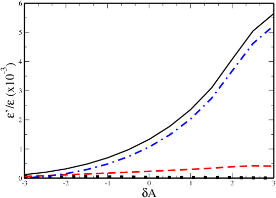
Figure 4: Contributions to $\varepsilon^{\prime}/\varepsilon$ versus the non–universality parameter $\delta A$. The dotted line refers to gluino contributions, the dott-dashed and dashed lines to the chargino one (with one and two mass insertions, respectively). The solid line stands for the total supersymmetric contribution to $\varepsilon^{\prime}/\varepsilon$.

As can be seen from this figure, the chargino contributions with one mass insertion give the dominant contribution to $\varepsilon^{\prime}/\varepsilon$. The chargino contributions with two mass insertions that arise from the SUSY effective $\bar{s}dZ$ vertex are also relevant and considerably larger than that of the gluino.

4 Small CP phases versus large CP asymmetry $a_{J/\psi K_{S}}$

For a long time all experimental evidence of CP violation was confined to the kaon sector. However, recent results from the $B$–factories have confirmed the existence of CP violation in the $B$ sector as well. The fact that the asymmetry $a_{J/\psi K_{S}}$ is large may lead to the conclusion that CP cannot be viewed as an approximate symmetry. We will show next that this is not necessarily true. In fact, it might happen that models with small CP violating phases but with a considerably large flavour mixing can also account for the recent experimental results. As it was shown in previous sections, supersymmetric USY models are indeed an example of this class of models, where a large flavour mixing and small CP phases still succeed in saturating the measured values of the CPV observables. In this section we address some of the implications of supersymmetric USY models for the $B$–system.

Regarding the CP asymmetry of the $B_{d}$ and $\bar{B}_{d}$ meson decay to the CP eigenstate $J/\psi K_{S}$, defined by

$$a_{J/\psi K_{S}}(t)=\frac{\Gamma(B_{d}(t)\to\psi K_{S})-\Gamma(\bar{B}_{d}(t)\to\psi K_{S})}{\Gamma(B_{d}(t)\to\psi K_{S})+\Gamma(\bar{B}_{d}(t)\to\psi K_{S})}=-a_{J/\psi K_{S}}\sin(\Delta m_{B_{d}}t)\;,$$ (72)

BaBar and Belle give the following results

$$a_{J/\psi K_{S}} =0.741\pm 0.067\pm 0.034\quad\quad\mathrm{(BaBar)}\;,$$

$$a_{J/\psi K_{S}} =0.719\pm 0.074\pm 0.035\quad\quad\mathrm{(Belle)}\;,$$ (73)

which dominate the present world average, $a_{J/\psi K_{S}}=0.734\pm 0.054$ [10, 11, 40].

In the case of the Standard Model, $a_{J/\psi K_{S}}$ can be easily related to one of the inner angles of the unitarity triangle:

$$a_{J/\psi K_{S}}^{SM}=\sin 2\beta\;;\quad\beta\equiv\arg\left(-\frac{{V}_{cd}{V}_{cb}^{*}}{{V}_{td}{V}_{tb}^{*}}\right)\;.$$ (74)

In the USY ansatz of Eq. (21), SM contributions to $\sin 2\beta$ are negligible, $\mathcal{O}(10^{-3})$. In view of this, it is mandatory that new physics provides a large contribution to $B_{d}-\bar{B}_{d}$.

In the case of supersymmetric contributions to the $\Delta B=2$ transition, the off–diagonal element of the $B_{d}$ mass matrix can be written as

$$M_{12}(B_{d})=\frac{\langle B_{d}|\mathcal{H}_{\mathrm{eff}}^{\Delta B=2}|\bar{B}_{d}\rangle}{2m_{B_{d}}}=M_{12}^{\mathrm{SM}}(B_{d})+M_{12}^{\mathrm{SUSY}}(B_{d}).$$ (75)

The supersymmetric effects are usually parametrised through

$$r_{d}^{2}e^{2i\theta_{d}}=\frac{M_{12}(B_{d})}{M_{12}^{\mathrm{SM}}(B_{d})},$$ (76)

where $\Delta m_{B_{d}}=2|M_{12}^{\mathrm{SM}}(B_{d})|r_{d}^{2}$. Thus, in the presence of SUSY contributions, the CP asymmetry parameter is now given by

$$a_{J/\psi K_{S}}=\sin(2\beta+2\theta_{d})\;.$$ (77)

Hence, the measurement of $a_{J/\psi K_{S}}$ would not determine $\sin 2\beta$ but rather $\sin(2\beta+2\theta_{d})$.

In many models, the SUSY contribution can be sufficient to account for the observed values of $a_{J/\psi K_{S}}$. However, this requires a large mixing in the $LL$ and $LR$ sectors, and this is indeed what we have in our USY example. As emphasized above, due to the large mixing in the USY textures, the non–universal $A$–terms have a non-negligible effect in the running of the squark masses and although we imposed universality of the scalar soft masses at the GUT scale, one finds considerable off diagonal contributions at the electroweak scale, particularly associated with mixtures of the third generation with the first two. Since in this class of models flavour mixing is not supressed, one finds that the $(\delta^{d,u}_{13})_{LL}$ and $(\delta^{d,u}_{13})_{LR}$ mass insertions (the most relevant in the $a_{J/\psi K_{S}}$ calculation) can be significantly large and saturate the experimental result as we show in detail below. In our numerical analysis, we took into account charged–Higgs, chargino and gluino contributions to $M_{12}^{\mathrm{SUSY}}(B_{d})$, as given in Ref. [41]. The leading supersymmetric contribution to $\sin(2\beta+2\theta_{d})$ is associated with the $\Delta B=2$ chargino mediated box diagrams. Instead of using the mass insertion approximation, as done in the previous sections, we choose to compute the full contibutions to $M_{12}^{\tilde{\chi}^{\pm}}(B_{d})$. The off–diagonal element of the $B_{d}$ mass matrix is accordingly given by:

$$M_{12}^{\tilde{\chi}^{\pm}}(B_{d}) = \frac{\alpha_{W}^{2}}{16}\frac{2}{3}f_{B}^{2}B_{B_{d}}\eta^{-6/23}m_{B_{d}}\sum_{h,k=1}^{6}\sum_{i,j=1}^{2}\frac{1}{m_{\tilde{\chi_{j}}^{\pm}}^{2}}\left\{\left[V^{*}_{j1}\;\Gamma_{U_{L}}^{kb}-V^{*}_{j2}\;{(\Gamma_{U_{R}}\;\hat{Y}_{U}\;K)}_{kb}\right]\right.$$ (78)

$$\left[V_{i1}\;{\Gamma^{U_{L}}}^{*}_{kd}-V_{i2}\;{(\Gamma^{U_{R}}\;\hat{Y}_{U}\;K)}^{*}_{kd}\right]\left[V^{*}_{j1}\;\Gamma^{U_{L}}_{hb}-V^{*}_{j2}\;{(\Gamma_{U_{R}}\;\hat{Y}_{U}\;K)}_{hb}\right]$$

$$\left[V_{j1}\;{\Gamma^{U_{L}}}^{*}_{hd}-V_{j2}\;{(\Gamma^{U_{R}}\;\hat{Y}_{U}\;K)}^{*}_{hd}\right]G^{\prime}(x_{\tilde{u}_{k}\tilde{\chi_{j}}},x_{\tilde{u}_{h}\tilde{\chi_{j}}},x_{\tilde{\chi_{i}}\tilde{\chi_{j}}})\left.\right\}\;,$$

where $x_{ab}=(m_{a}/m_{b})^{2}$, $f_{B_{d}}$ is the $B_{d}$ meson decay constant, $B_{B_{d}}$ is the vacuum saturation parameter, and $\eta$ is the QCD correction factor. As before, $V$ is one of the unitary matrices that diagonalise the chargino mass matrix and $K$ is the CKM matrix. $\hat{Y_{U}}\equiv{\mathrm{diag}}(m_{u},m_{c},m_{t})/(\sqrt{2}m_{W}\sin\beta)$, $\Gamma_{U_{L,R}}$ are the matrices relating the squark interaction and mass eigenstates, and the loop function $G^{\prime}$ is given in Ref. [41]. In Fig. 5 we present the correlation between the values of $\varepsilon_{K}$ and $\sin 2\theta_{d}$ for $\tan\beta=5$ and $m_{0}=m_{1/2}=250$ GeV. The values of the parameters $a,b,$ and $c$ are randomly selected in the range $[-3,3]$ and the phases are fixed as $\varphi_{a}=\varphi_{c}=0$ and $\varphi_{b}=0.1$.

Figure 5: Correlation between $\varepsilon_{K}$ and $\sin 2\theta_{d}$. The crosses (+) correspond to values $a=b=-3$ and $c\in\left[-1.5,0.5\right]$.

From Fig. 5, it is clear that one can have $\sin 2\theta_{d}$ within the experimental range while having a prediction for $\varepsilon_{K}$ and $\varepsilon^{\prime}/\varepsilon$ compatible with the measured value. This result appears as a characteristic of the kind of models under consideration. Despite the smallness of the phases introduced in these models via the Yukawa and trilinear couplings, they are sufficient to account for CP violation in the $K$-system, as well as the observed value of $a_{J/\psi K_{S}}$, which requires a phase of order one.

It is worth mentioning that the non–universality of the $A$-terms is crucial for enhancing the SUSY contributions. As emphasized above, for universal $A$-terms the mass insertions $(\delta^{u}_{31})_{LL}$ and $(\delta^{u}_{13})_{LR}$ are, respectively, of order $10^{-5}$ and $10^{-6}$, leading to a negligible $\sin 2\theta_{d}$. When non–universal $A$-terms are considered, we find that the chargino contribution displays a large phase, while the gluino and SM contributions are almost real and in general smaller than the chargino contribution. The Higgs and neutralino contributions are negligible in the cases under consideration.

If we assume that the universality of the $A$-terms is broken by setting $a=b\neq c$ as in Eq. (37), it is possible to find sizable values for the the SUSY contributions to $a_{J/\psi K_{S}}$. In Fig. 5 we considered particular values of $a,\;b,\;c$, namely $a=b=-3$ and $c\in\left[-1.5,0.5\right]$, and marked the associated contributions to $\sin 2\theta_{d}$ and $\varepsilon_{K}$ with a cross ($+$). As seen from Fig. 5, for this set of points, $\sin 2\theta_{d}$ ranges from 0.99 to 0.3 while $\varepsilon_{K}$ takes values between $(1-3)\times 10^{-3}$. Regarding values of the relevant mass insertions, the values of $a,\;b,\;c$ corresponding to the crosses in Fig. 5, we find that $\sqrt{|\operatorname{Im}\left[(\delta^{u}_{LL})^{2}_{13}\right]|}$, $\sqrt{|\operatorname{Im}\left[(\delta^{u}_{RL})^{2}_{13}\right]|}$ and $\sqrt{|\operatorname{Im}\left[(\delta^{u}_{LL})_{13}\right]\operatorname{Im}\left[(\delta^{u}_{RL})_{13}\right]|}$, are of the same order of maginitude and range from 0.08 to 0.2 as $c$ varies from -1.5 to 0.5. The mass insertions $\sqrt{|\operatorname{Im}\left[(\delta^{u}_{LL})_{13}\right]\operatorname{Im}\left[(\delta^{u}_{LL})_{23}\right]|}$, $\sqrt{|\operatorname{Im}\left[(\delta^{u}_{RL})_{13}\right]\operatorname{Im}\left[(\delta^{u}_{RL})_{23}\right]|}$, $\sqrt{|\operatorname{Im}\left[(\delta^{u}_{LL})_{13}\right]\operatorname{Im}\left[(\delta^{u}_{RL})_{23}\right]|}$, take values from 0.065 to 0.12 in the same range.

We notice that the values of these mass insertions are compatible with those given in Ref. [42] to saturate the SUSY contributions to $a_{J/\psi K_{S}}$ . As a specific example, for $a=b=-3$ and $c=-0.9$ we find $\varepsilon_{K}=2\times 10^{-3}$, and $\sin 2\theta_{d}=0.7$. The most relevant mass insertion for the gluino contribution is: $(\delta^{d}_{31})_{LL}=-0.0012-0.066i$, being the other contributions below $10^{-5}$. The relevant mass insertions for the chargino contribution are $(\delta^{u}_{31})_{LL}=0.0014-0.087i$, $(\delta^{u}_{31})_{RL}=0.00051-0.11i$, $(\delta^{u}_{32})_{LL}=0.011+0.047i$ and $(\delta^{u}_{32})_{RL}=-0.018+0.059i$ .

Note that although we assume that $A^{u}=A^{d}$ at the GUT scale, due to the effect of the large top Yukawa in the evolution to the electroweak scale, one obtains $\operatorname{Im}[(\delta^{u}_{31})_{RL}]\approx 0.1$ while $\operatorname{Im}[(\delta^{d}_{31})_{RL}]\approx 10^{-5}$. Therefore, the chargino exchange gives the dominant contribution to $\sin 2\theta_{d}$.

To conclude this section, we address the $\Delta B=1$ process $b\to s\gamma$. As aforementioned, USY models have large mixing, hence one might expect that the mass insertions $(\delta^{d}_{23})_{LL}$ and $(\delta^{d}_{23})_{LR}$ receive large contributions, and this could lead to excessive values for the branching ratio (BR) of the $b\to s\gamma$ decay, above the experimental limit reported by the CLEO collaboration [43]:

$$2.0\times 10^{-4}<BR\;(B\rightarrow X_{s}\gamma)<4.5\times 10^{-4}\;.$$ (79)

The supersymmetric contributions to the process are given by the one–loop magnetic dipole and chromomagnetic dipole penguin diagrams, which are mediated by charged Higgs boson, chargino, gluino and neutralino exchanges.

It is known [44] that with universal $A$-terms, the gluino contribution is very small and the leading ones are those involving the charged Higgs and charginos. In this case, and for our choice of USY phases, we found that the total $BR\;(B\rightarrow X_{s}\gamma)\;\simeq 3.5\times 10^{-4}$, which is essentially the SM central value. For the case of non-universal trilinear terms, we present just an illustrative example. Let us consider (for the structure given in Eq. (37)), $a=-1.7,b=c=-3$, a point in parameter space associated with a nearly maximal value of $\sin(2\beta+2\theta_{d})$. In this case $BR\;(B\rightarrow X_{s}\gamma)\;\simeq 2.8\times 10^{-4}$, still in agreeement with SM results, as discussed in Ref.[44].

5 Discussion and Conclusions

In this work we have studied the implications of having universal strength of Yukawa couplings within the MSSM. This class of ansätze for the quark mass matrices is specially interesting since it provides a relationship between the observed pattern of quark masses and mixings and the possibility of having small CP violating phases. We have addressed the problem of CP violation in supersymmetric USY models, showing that the strength of CP violation due to the standard KM mechanism is too small to account for the observed CP violation, and essential contributions from supersymmetry are required.

We have shown that the trilinear soft terms play a key rôle in embedding USY into SUSY. In fact, due to the large mixing and associated phases, the constraints from the EDMs on the SUSY parameter space are far more stringent than in the case of a standard Yukawa parametrization. Although the effect of these phases is absent in the SM and in SUSY models with flavour conserving soft breaking terms, once we require a non–universality in the trilinear terms (which proves to be essential to saturate the CP observables) there are large contributions to the electric dipole moments of the neutron and mercury atom. We found that in order to satisfy the bound of the mercury EDM the $A$–terms should be matrix factorizable, and their phases constrained to be of order $10^{-2}-10^{-1}$.

Within the region of the supersymmetric parameter space where one had compatibility with the EDM measurements, we have investigated the new contributions to both K and $B$ system CP observables, and we have shown that in the present model it is possible to saturate the experimental values of $\varepsilon_{K}$ and $\varepsilon^{\prime}/\varepsilon$. Gluino mediated boxes with $LL$ mass insertions provide the leading contributions to $\varepsilon_{K}$, while $\varepsilon^{\prime}/\varepsilon$ is dominated by chargino loops, through $LL$ flavour mixing.

Finally, we considered the CP asymmetry of the $B$ meson decay, $a_{J/\psi K_{S}}$. It turns out that within this model the SM contribution to this asymmetry is negligible, while supersymmetry, namely through chargino exchange, provides the leading contributions, which are in agreement with the recent measurements at BaBar and Belle.

In conclusion, we have presented an alternative scenario for CP violation, where the strength of CP violation originated from the SM is naturally small, due to the observed pattern of quark masses and mixing angles, which constrain all USY phases to be small. We have shown that in this framework new SUSY contributions are essential in order to generate the correct value of $\varepsilon_{K}$ and $\varepsilon^{\prime}/\varepsilon$, as well as the recently observed large value of $a_{J/\psi K_{S}}$.

Acknowlegdments

S.K. would like to thank CFIF for its kind hospitality during the final stage of this work. We are grateful to F. Joaquim and K. Tamvakis for useful discussions. This work was supported in part by the Portuguese Ministry of Science through project CERN/P/Fis/40134/2000, CERN/P/Fis/43793/2001, and by the E.E. through project HPRN-CT-2000-001499. M.G. and A.T. acknowledge support from ’Fundacão para a Ciência e Tecnologia’, under grants SFRH/BPD/5711/2001 and PRAXIS XXI BD/11030/97, respectively. The work of S.K. was supported by PPARC.

Appendix: USY and a local horizontal symmetry

In this appendix we show how USY textures can be motivated by a horizontal symmetry. For instance, with the horizontal gauge group $SU(3)_{H}\times U(1)_{H}$, the matter content of the MSSM can be assigned as $\{Q_{a},L_{a}\}\equiv(3,1)~{}\mathrm{and}~{}\{u^{c}_{a},\;d^{c}_{a},\;e^{c}_{a}\}\equiv(\bar{3},-1)\;,$ while the charges of the MSSM Higgs are given by $\{H_{u},H_{d}\}\equiv(1,0)$. The extra Higgs fields that may be used to break $SU(3)_{H}\times U(1)_{H}$ are $\phi_{a}\equiv(3,1)$ and $\bar{\phi}^{a}\equiv(\bar{3},-1)$, $a=1,2,3$. We introduce an additional $Z_{4}$ discrete symmetry, under which $\{H_{u},H_{d}\}\rightarrow\{-H_{u},-H_{d}\}$, $\{{\phi_{a},\bar{\phi}^{a}}\}\rightarrow\{{i\phi_{a},i\bar{\phi}^{a}\}}$, while all other matter superfields transform trivialy. This symmetry prevents the presence of renormalizable terms involving quarks and leptons in the superpotential. Therefore, the lowest dimensional $SU(3)_{H}\times U(1)_{H}$ invariant operators in the superpotential, which are responsible for generating the fermion masses, are given by

$$W_{\mathrm{Yuk}}=h_{u}Q_{a}u^{c}_{b}H_{u}\frac{\bar{\phi}^{a}\phi_{b}}{M^{2}}+h_{d}Q_{a}d^{c}_{b}H_{d}\frac{\bar{\phi}^{a}\phi_{b}}{M^{2}}+h_{l}L_{a}e^{c}_{b}H_{d}\frac{\bar{\phi}^{a}\phi_{b}}{M^{2}},$$ (A2)

where $M$ is a scale much higher than the weak scale. The minimization of the scalar potential involving the fields ($\bar{\phi}^{a},\ \phi^{b}$) can be derived in a similar way as in Refs. [27, 45]. Thus $Y^{u}_{ab}=h_{u}\frac{\bar{v}^{a}v^{b}}{M^{2}}$, where $\bar{v}^{a}$, $v^{b}$ are the vacuum expectation values of $\bar{\phi}^{a}_{i}=\bar{v}^{a}\delta_{ai}$ and $\phi^{b}=v^{b}\delta_{bi}$ ($i=1,2,3$), respectively. In fact, for a particular choice of the soft terms associated to the fields ($\bar{\phi}^{a},\ \phi^{b}$) one can assume that if $v^{a}$ and $\bar{v}^{b}$ are given by $v^{a}=|v|e^{i\varphi_{a}}$ and $\bar{v}^{b}=|v|e^{i\varphi^{\prime}_{b}}$, then

$$Y_{ab}^{u}=h^{\prime}_{u}\;e^{i(\varphi_{a}+\varphi^{\prime}_{b})}\;,\quad\mathrm{with}\quad h^{\prime}_{u}=\frac{h_{u}{|v|}^{2}}{M^{2}}\;.$$ (A3)

Similar expressions hold for $Y^{d}$ and $Y^{l}$. The Yukawa couplings in Eq. (A3) clearly display the usual USY form, which was discussed in section 2.

References

• [1] A.G. Cohen, D.B. Kaplan and A.E. Nelson, Annu. Rev. Nucl. Part. Sci. 43 (1993) 27; M.B. Gavela, P. Hernandez, J. Orloff, O. Pène and C. Quimbay, Mod. Phys. Lett. A 9 (1994) 795 and Nucl. Phys. B 430 (1994) 382; A.D. Dolgov, hep-ph/9707419; V.A. Rubakov and M.E. Shaposhnikov, Usp. Fiz. Nauk 166 (1996) 493 [Phys. Usp. 39 (1996) 461].
• [2] S. Abel, S. Khalil and O. Lebedev, Nucl. Phys. B 606 (2001) 151.
• [3] S. Pokorski, J. Rosiek and C. A. Savoy, Nucl. Phys. B 570 (2000) 81
• [4] Recent Developments in Gauge Theories, Proceedings of Nato Advanced Study Institute (Cargèse, 1979), edited by G. ’t Hooft et al., Plenum, New York (1980).
• [5] G. C. Branco, J. I. Silva-Marcos and M. N. Rebelo, Phys. Lett. B 237 (1990) 446; G. C. Branco, D. Emmanuel–Costa and J. I. Silva-Marcos, Phys. Rev. D56 (1997) 107.
• [6] P. M. Fishbane and P. Q. Hung, Phys. Rev. D57 (1998) 2743.
• [7] P. Q. Hung and M. Seco, hep-ph/0111013.
• [8] G. C. Branco and J. I. Silva-Marcos, Phys. Lett. B 359 (1995) 166.
• [9] M. V. Romalis, W. C. Griffith and E. N. Fortson, Phys. Rev. Lett. 86 (2001) 2505; J. P. Jacobs et al. Phys. Rev. Lett. 71 (1993) 3782.
• [10] BABAR Collaboration, B. Aubert et al., Phys. Rev. Lett. 89 (2002) 201802.
• [11] BELLE Collaboration, K. Abe et al., Phys. Rev. D66 (2002) 071102.
• [12] G. Eyal and Y. Nir, Nucl. Phys. B 528 (1998) 21, and references therein.
• [13] G. C. Branco, F. Cagarrinho and F. Krüger, Phys. Lett. B 459 (1999) 224
• [14] H. Fritzsch and J. Plankl, Phys. Rev. D49 (1994) 584; H. Fritzsch and P. Minkowski, Nuovo Cim. 30A (1975) 393; H. Fritzsch and D. Jackson, Phys. Lett. B 66 (1977) 365; P. Kaus and S. Meshkov, Phys. Rev. D42 (1990) 1863.
• [15] H. Fusaoka and Y. Koide, Phys. Rev. D57 (1998) 3986.
• [16] See for example, V. Barger, M. S. Berger and P. Ohmann, Phys. Rev. D47 (1993) 1093; ibid. 49 (1994) 4908.
• [17] G. C. Branco and J. I. Silva-Marcos, Phys. Lett. B 331 (1994) 390.
• [18] Particle Data Group, Eur. Phys. J. C 15 (2000) 1.
• [19] C. Jarlskog, Phys. Rev. Lett. 55 (1985) 1039; Z. Phys. C 29 (1985) 491.
• [20] C. Liu, Int. J. Mod. Phys. A 11 (1996) 4307.
• [21] M. Dugan, B. Grinstein and L. J. Hall, Nucl. Phys. B 255 (1985) 413.
• [22] D. A. Demir, A. Masiero and O. Vives, Phys. Lett. B 479 (2000) 230; S. M. Barr and S. Khalil, Phys. Rev. D61 (2000) 035005.
• [23] A. Brignole, L. E. Ibanez and C. Munoz, Nucl. Phys. B 422 (1994) 125; Erratum ibid. 4361995747; A. Brignole, L. E. Ibanez, C. Munoz and C. Scheich, Z. Phys. C 74 (1997) 157.
• [24] S. A. Abel and J. M. Frère, Phys. Rev. D55 (1997) 1632; S. Khalil, T. Kobayashi and A. Masiero, Phys. Rev. D60 (1999) 075003; S. Khalil and T. Kobayashi, Phys. Lett. B 460 (1999) 341.
• [25] S. Khalil, T. Kobayashi and O. Vives, Nucl. Phys. B 580 (2000) 275; T. Kobayashi and O. Vives, Phys. Lett. B 506 (2001) 323.
• [26] S. Abel, D. Bailin, S. Khalil and O. Lebedev, Phys. Lett. B 504 (2001) 241.
• [27] S. Khalil, JHEP 0212 (2002) 012.
• [28] A. Masiero, M. Piai, A. Romanino and L. Silvestrini, Phys. Rev. D64 (2001) 075005, and references therein.
• [29] P. G. Harris et al, Phys. Rev. Lett. 82 (1999) 904.
• [30] M. Ciuchini et al, J. High Energy Phys. 10 (1998) 008.
• [31] S. Khalil and O. Lebedev, Phys. Lett. B 515 (2001) 387.
• [32] A. J. Buras, hep-ph/0101336.
• [33] See, for example, G. C. Branco, L. Lavoura and J. P. Silva, CP Violation, International Series of Monographs on Physics (103), Oxford University Press, Clarendon (1999).
• [34] F. Gabbiani, E. Gabrielli, A. Masiero and L. Silverstrini, Nucl. Phys. B 477 (1996) 321.
• [35] V. Fanti et al, Phys. Lett. B 465 (1999) 335.
• [36] T. Gershon (NA48), hep-ex/0101034.
• [37] A. J. Buras, M. Jamin and M. E. Lautenbacher, Nucl. Phys. B 408 (1993) 209.
• [38] S. Bertolini, M. Fabbrichesi and E. Gabrielli Phys. Lett. B 327 (1994) 136.
• [39] G. Colangelo and G. Isidori J. High Energy Phys. 09 (1998) 009; A. Buras, G. Colangelo, G. Isidori, A. Romanino and L. Silvestrini Nucl. Phys. B 566 (2000) 3
• [40] OPAL Collaboration, K. Ackerstaff et al , Eur. Phys. J. C 5 (1998) 379; CDF Collaboration, T. Affolder et al, Phys. Rev. D61 (2000) 072005; CDF Collaboration, C. A. Blocker, Proceedings of 3rd Workshop on Physics and Detectors for DAPHNE (DAPHNE 99), Frascati, Italy, 16-19 Nov 1999; ALEPH Collaboration, R. Barate et al, Phys. Lett. B 492 (2000) 259.
• [41] S. Bertolini, F. Borzumati, A. Masiero and G. Ridolfi, Nucl. Phys. B 353 (1991) 591.
• [42] E. Gabrielli and S. Khalil, Phys. Rev. D 67 (2003) 015008.
• [43] CLEO Collaboration, S. Ahmed et al, CLEO-CONF-99-10, hep-ex/9908022.
• [44] E. Gabrielli, S. Khalil and E. Torrente–Lujan, Nucl. Phys. B 594 (2001) 3.
• [45] K. S. Babu and R. N. Mohapatra, Phys. Rev. Lett. 83 (1999) 2522