Precise calculation of parity nonconservation in cesium and test of the standard model

Abstract

We have calculated the $6s-7s$ parity nonconserving (PNC) E1 transition amplitude, $E_{PNC}$, in cesium. We have used an improved all-order technique in the calculation of the correlations and have included all significant contributions to $E_{PNC}$. Our final value $E_{PNC}=0.904\Big{(}1\pm 0.5\%\Big{)}\times 10^{-11}iea_{B}(-Q_{W}/N)$ has half the uncertainty claimed in old calculations used for the interpretation of Cs PNC experiments. The resulting nuclear weak charge $Q_{W}$ for Cs deviates by about $2\sigma$ from the value predicted by the standard model.

I Introduction

There is an ongoing discussion on whether measurements of parity nonconservation (PNC) in atoms can be used to study new physics beyond the standard model (for a history of PNC in atoms, see, e.g., the book [1] or review [2]). Such a possibility relies on the accuracy of the measurements and the theoretical analysis. The best accuracy so far has been achieved for the cesium atom. In 1997, the Boulder group measured the PNC amplitude in cesium to an accuracy of 0.35% [3]. The best calculations available at that time were published by the Novosibirsk group in 1989 [4] and the Notre Dame group in 1990 [5]. Both works claimed an accuracy of 1%. This claim of 1% accuracy was based in part on the comparison of the experimental and theoretical values relevant to the PNC amplitude (energies, electromagnetic E1 transition amplitudes, hyperfine structure). Later, new, more accurate measurements (see, e.g. [6, 7]) led to better agreement between theory and experiment for the E1 transition amplitudes. This allowed Bennett and Wieman to suggest that the actual accuracy of the PNC calculations in cesium is 0.4% [8]. With this accuracy, the value of the nuclear weak charge $Q_{W}$ of the cesium atom which follows from the measurements [3] and calculations [4, 5] deviates from the standard model value by $2.5\sigma$ [8]. The implications of this deviation for physics beyond the standard model have been examined in several works [9, 10, 11].

This result generated many recent works revisiting calculations of PNC in cesium. Derevianko [12] demonstrated that the contribution of the Breit interaction to the PNC amplitude $E_{PNC}$ (-0.6%) is substantially larger than previous estimates and reduces the deviation from the standard model. The Breit contribution was neglected in [4] and underestimated in [5]. The result of Derevianko was later confirmed in independent calculations [13, 14]. A new many-body calculation of $E_{PNC}$ was performed by Kozlov et al. [14]. It was calculated in second-order in the residual interaction with averaged screening factors. The result is in excellent agreement with similar calculations by Blundell et al. [5] and differs by less than 0.5% from the more complete (“all-orders”) calculations [4, 5].

Radiative corrections to the weak charge of order $\alpha$ were calculated a long time ago in [15] (see also [16]). However, there are important “strong field” radiative corrections of order $Z\alpha^{2}$ and $Z^{2}\alpha^{3}\ln^{2}(\lambda/R_{n})$ which have recently been considered in [17] (note that the latter correction is larger). Here $\lambda$ is the electron Compton wavelength, and $R$ is the nuclear radius. The main contribution to $E_{PNC}$ was found to be about $0.4\%$. This contribution originates from the radiative corrections to the weak matrix element due to the Uehling potential (recently this contribution was calculated numerically in [18]).

Among other corrections considered one should mention a correction for the neutron distribution [19] which is quite small: -0.2% of $E_{PNC}$.

Note that Breit, Uehling, and neutron skin corrections are smaller than the uncertainty of 1% claimed for the calculated $E_{PNC}$ amplitude in works [4, 5]. This uncertainty was mostly associated with the accuracy of the calculations of correlation corrections. Therefore, there is a very important question as to whether calculations of correlations were, or can be, performed to better than 1% accuracy. The analysis of the accuracy involves a comparison of calculated and measured atomic quantities and some additional “internal” tests, such as, e.g., checking the stability of the results against variation of certain parameters. Comparison with experiment alone is an important but not sufficient part of the analysis. This is especially true when better accuracy is claimed for calculations performed many years ago and all the details can hardly be reconstructed. In our view, the only reliable way to improve the accuracy is to do the calculations again, trying to improve the method and numerical procedures at every stage, and repeat the analysis of the accuracy. That is what we do in the present paper.

We have made several important improvements to the method developed in 1989 [4]. First, we calculated a new series of higher-order correlation diagrams which account for the effect of screening of the Coulomb interaction in the exchange correlation diagram. In our earlier work [4] the screening effect was calculated for the direct correlation diagram only, while screening factors were used for the exchange diagram. The values of these factors were found by looking at the effect of screening in the direct diagram; however, the effect of screening in the exchange diagram may differ. In our present work we calculate the effect of screening for both diagrams.

Second, we have made significant improvements to the numerical procedures at every stage of the calculations. This involves, for instance, using a more dense coordinate grid, including more terms into the summation over virtual states, and restoring the lower Dirac component of the wave function everywhere. We have also used a more accurate nuclear charge distribution.

Our result for the PNC amplitude in cesium (without Breit, radiative, and neutron distribution corrections) $E_{PNC}=0.908\Big{(}1\pm 0.5\%\Big{)}\times 10^{-11}iea_{B}(-Q_{W}/N)$ coincides exactly with the old result [4] but has a much smaller uncertainty. ($N$ is the neutron number.) To avoid misunderstanding, we should note that particular contributions to this value are slightly different in the old and the new calculations (for example, the Hartree-Fock value of the amplitude has changed by 0.3%). Therefore, we are indeed talking about a new result.

We have also calculated the contributions of the Breit interaction (-0.61%) and the Uehling potential (0.40%) to $E_{PNC}$. There is very good agreement between different calculations for these values and they can be considered well-established. The resulting value for the PNC amplitude is $E_{PNC}=0.906\Big{(}1\pm 0.5\%\Big{)}\times 10^{-11}iea_{B}(-Q_{W}/N)$. The neutron-distribution correction, estimated as $(-0.2\pm 0.1)\%$, reduces our final value to $E_{PNC}=0.904\Big{(}1\pm 0.5\%\Big{)}\times 10^{-11}iea_{B}(-Q_{W}/N)$.

II Method of calculation

The method we have used here is very similar to that used in our 1989 work [4]. As a zero approximation we use the relativistic Hartree-Fock method. The perturbation in our approach is the residual interaction - the difference between the exact and Hartree-Fock Hamiltonians. For summing of diagrams we use a combination of the “correlation potential method” [23], which is a way to treat correlations by introducing a single-electron operator (correlation potential) $\hat{\Sigma}$, and “perturbation theory in the screened electron residual interaction” [24, 25], which is used to calculate $\hat{\Sigma}$. The method is an all-order technique, in terms of treating correlations, and is not a version of the popular coupled-cluster approach. The dominating sequences of higher-order correlation diagrams correspond to real physical phenomena like collective screening of the Coulomb interaction between electrons and the hole-particle interaction. They are included in all orders in our technique. An important strong point of the method is that its complexity does not go beyond the calculation of the correlation potential $\hat{\Sigma}$. When $\hat{\Sigma}$ is ready, the calculation of energies and matrix elements is relatively simple. $\hat{\Sigma}$ is used to calculate single-electron Brueckner orbitals. The calculation of matrix elements with Brueckner orbitals already includes most of the correlations. There are additional “non-Brueckner” contributions to matrix elements such as structural radiation and normalization of many-electron states. These contributions are small for $s$ and $p$ states and in most cases they can be expressed in terms of derivatives of $\hat{\Sigma}$. This makes the calculation of hyperfine structure, transition amplitudes, etc. similar to the calculation of energies.

The method works very well for alkaline atoms. The calculated energy levels and transition amplitudes deviate by a fraction of a percent from experiment. The hyperfine structure (hfs) of $s$ and $p$ states has an accuracy of better than 1%.

A Correlation potential method

The Cs atom has one electron above closed shells. Therefore, it is natural to start the calculations from the relativistic Hartree-Fock (RHF) method in the $\hat{V}^{N-1}$ approximation (one electron in the field of the $N-1$ core electrons). The single-electron RHF Hamiltonian is

$$\hat{H}_{0}=c\mbox{\boldmath$\alpha$}\cdot\hat{{\bf p}}+(\beta-1)c^{2}-Z\alpha/r+\hat{V}^{N-1}\ ,$$ (1)

$\alpha$ and $\beta$ are Dirac matrices and $\hat{{\bf p}}$ is the electron momentum. For cesium the accuracy of the RHF energies is of the order of $10\%$.

To improve the accuracy one needs to include correlations. In order to do so we introduce a “correlation potential” $\hat{\Sigma}$ [23]. $\hat{\Sigma}$ is a single-electron energy-dependent non-local operator defined in such a way that its average value over a single-electron state $a$ is the correlation correction to the energy of this state,

$$\Delta\epsilon_{a}=\langle a|\hat{\Sigma}(\epsilon_{a})|a\rangle.$$ (2)

The calculation of $\hat{\Sigma}$ will be described in the next section. $\hat{\Sigma}$ is added to the Hartree-Fock Hamiltonian to calculate single-electron states of the external electron,

$$(\hat{H}_{0}+\hat{\Sigma}-\epsilon)\psi^{\rm Br}=0.$$ (3)

There are two major benefits from inclusion of $\hat{\Sigma}$ in the equations. First, the iteration of $\hat{\Sigma}$ is an important higher-order effect which gives a significant contribution to the energy and wave function. Second, by solving Eq. (3) we obtain single-electron orbitals which are called Brueckner orbitals which already include correlations. These orbitals can then be used to calculate matrix elements for hfs, PNC, etc.

When appropriate higher-order diagrams are included into the calculation of $\hat{\Sigma}$, as will be described in the next section, by solving Eq. (3) we obtain energies of $s$ and $p$ states of alkaline atoms with an accuracy of about 0.1%. This is a radical improvement over the 10% accuracy of the Hartree-Fock approximation.

To accurately calculate the interaction of external fields with atomic electrons one needs also to take into account the core polarization effect. We do this using the time-dependent Hartree-Fock (TDHF) method (which is equivalent to the random-phase approximation with exchange). In this method every single-electron orbital has the form

$\displaystyle\psi_{n}+\delta\psi_{n}\ ,$where $\psi_{n}$ is the unperturbed Hartree-Fock orbital (or Brueckner one for states above the core) and $\delta\psi_{n}$ is a correction to the orbital caused by the external field. To find $\delta\psi_{n}$ one needs to solve the equations

$$(\hat{H}_{0}-\epsilon)\delta\psi_{n}=-(\delta\epsilon+\hat{h}+\delta\hat{V}_{h})\psi_{n}.$$ (4)

Here $\hat{h}$ is the operator of the external field, $\delta\hat{V}_{h}$ is the correction to the Hartree-Fock potential due to modification of the core states in the external field, and $\delta\epsilon$ is the correction to the energy.

Equations (4) are first solved self-consistently for core states to obtain $\delta\hat{V}_{h}$. Then Brueckner orbitals are used to calculate matrix elements between states of the external electron

$$M_{ab}=\langle\psi^{\rm Br}_{b}|\hat{h}+\delta\hat{V}_{h}|\psi^{\rm Br}_{a}\rangle.$$ (5)

This expression includes most of the correlations and already gives hfs and transition amplitudes in alkaline atoms to an accuracy close to 1%. There are also contributions arising from the normalization of states and structural radiation [23]. When these contributions are included the accuracy improves.

B Calculation of the correlation potential

We use the Feynman diagram technique to calculate the correlation potential $\hat{\Sigma}$. The main reason for this is that this technique is more convenient for inclusion of higher-order diagrams. The drawback of it is the necessity to integrate over frequencies numerically.

In the lowest (second) order in the residual Coulomb interaction, $\hat{\Sigma}$ is given by the direct and exchange diagrams in Fig. 1. The corresponding mathematical expressions are

$$\hat{\Sigma}^{(2)}_{\rm d}(\epsilon,r_{i},r_{j}) = \sum_{nm}\int\frac{d\omega}{2\pi}G_{ij}(\epsilon+\omega)\hat{Q}_{im}\hat{\Pi}_{mn}(\omega)\hat{Q}_{nj},$$ (6)

$$\hat{\Sigma}^{(2)}_{\rm ex}(\epsilon,r_{i},r_{j}) = \sum_{mn}\int\int\frac{d\omega_{1}}{2\pi}\frac{d\omega_{2}}{2\pi}\hat{Q}_{in}G_{im}(\epsilon+\omega_{1})G_{mn}(\epsilon+\omega_{1}+\omega_{2})\hat{Q}_{mj}G_{nj}(\epsilon+\omega_{2}),$$ (7)

where summation over $m$ and $n$ is a numerical implementation of the integration over $r_{m}$ and $r_{n}$, $\hat{Q}$ is the Coulomb interaction, $G$ is the Hartree-Fock Green function, $\hat{\Pi}$ is the polarization operator:

$$\hat{Q}_{ij}=\frac{e^{2}}{|r_{i}-r_{j}|},$$ (8)

$$G_{ij}(\epsilon)=\sum_{\gamma}\frac{|\gamma\rangle_{i}\langle\gamma|_{j}}{\epsilon-\epsilon_{\gamma}+i\delta}+\sum_{n}\frac{|n\rangle_{i}\langle n|_{j}}{\epsilon-\epsilon_{n}-i\delta},\ \ \delta\rightarrow 0,$$ (9)

$$\hat{\Pi}_{ij}(\omega)=\int\frac{d\alpha}{2\pi}G_{ij}(\omega+\alpha)G_{ij}(\alpha)=\sum_{n}\psi_{n}^{\dagger}\big{(}G_{ij}(\epsilon_{n}+\omega)+G_{ij}(\epsilon_{n}-\omega)\big{)}\psi_{n}.$$ (10)

Here $|n\rangle$ are core RHF states and $|\gamma\rangle$ are RHF excited states; $\delta$ shows the pole passing rule for integration over frequencies. (Let us remind the reader that we use the Feynman diagram technique to treat a basically non-relativistic correlation problem, e.g., our polarization operator (10) represents the polarization of the atomic core, not the vacuum.)

The integration over frequencies in expressions (6) and (7) can easily be performed analytically, reducing the diagrams in Fig. 1 to the four usual Goldstone diagrams presented, e.g., in work [23]. When higher-orders are included in $\hat{\Sigma}$, only the integration for the polarization operator (10) can still be done analytically. The other integrals have to be calculated numerically.

As was demonstrated in our earlier work [24], the most important higher-order correlation contributions to $\hat{\Sigma}$ come from screening of the Coulomb interaction between atomic electrons by other electrons and from the hole-particle interaction in the polarization operator (another important higher-order effect is the iteration of $\hat{\Sigma}$, which is included separately, by inserting $\hat{\Sigma}$ into equations for single-electron orbitals; see previous section).

The hole-particle interaction in the polarization operator $\hat{\Pi}$ (Fig. 2) is included by replacing the $\hat{V}^{N-1}$ Hartree-Fock potential in the calculation of $\hat{\Pi}$ by the $\hat{V}^{N-2}$ potential. Since the calculation involves iterations of the RHF equation, the hole-particle interaction is included in all orders.

The screening of the Coulomb interaction is a more complicated effect. The corresponding higher-order diagrams can be obtained from the second-order diagrams (Fig. 1) by the insertion of a series of hole-particle loops into every Coulomb line. Therefore, instead of, e.g., one direct diagram (Fig. 1) we have an infinite chain of higher-order diagrams (Fig. 3). One can see that an internal part of this chain (before the integration over $\omega$) forms a matrix geometric progression

$\displaystyle\hat{\Pi}+\hat{\Pi}\hat{Q}\hat{\Pi}+\hat{\Pi}\hat{Q}\hat{\Pi}\hat{Q}\hat{\Pi}+\dots$The sum of this progression is

$$\hat{\pi}(\omega)=\hat{\Pi}(\omega)\big{[}1-\hat{Q}\hat{\Pi}(\omega)\big{]}^{-1},$$ (11)

and can be called the “screened polarization operator”. Screening of the Coulomb interaction in the direct correlation diagram is included by replacing the unscreened polarization operator $\hat{\Pi}$ in Eq. (6) by the screened polarization operator $\hat{\pi}$:

$$\hat{\Sigma}_{\rm d}(\epsilon,r_{i},r_{j}) = \sum_{nm}\int\frac{d\omega}{2\pi}G_{ij}(\epsilon+\omega)\hat{Q}_{im}\hat{\pi}_{mn}(\omega)\hat{Q}_{nj}.$$ (12)

It is convenient also to introduce an operator of the screened Coulomb interaction

$$\widetilde{Q}(\omega)=\hat{Q}(1-\hat{Q}\hat{\pi}(\omega))^{-1}.$$ (13)

This expression can be obtained in a similar way to the screened polarization operator $\hat{\pi}$ by summing a matrix geometric progression corresponding to the chain of diagrams in Fig. 4. An expression for the direct correlation diagram can be re-written in terms of $\widetilde{Q}$:

$$\hat{\Sigma}_{\rm d}(\epsilon,r_{i},r_{j}) = \sum_{nm}\int\frac{d\omega}{2\pi}G_{ij}(\epsilon+\omega)\hat{Q}_{im}\hat{\Pi}_{mn}(\omega)\widetilde{Q}_{nj}(\omega).$$ (14)

The screened Coulomb interaction operator $\widetilde{Q}$ can also be used to include screening into the exchange correlation diagram. This is done by substituting $\hat{Q}\rightarrow\widetilde{Q}(\omega)$ in equation (7)

$$\hat{\Sigma}_{\rm ex}(\epsilon,r_{i},r_{j})=$$ (15)

$$\sum_{mn}\int\int\frac{d\omega_{1}}{2\pi}\frac{d\omega_{2}}{2\pi}\widetilde{Q}_{in}(\omega_{1})G_{im}(\epsilon+\omega_{1})G_{mn}(\epsilon+\omega_{1}+\omega_{2})\widetilde{Q}_{mj}(\omega_{2})G_{nj}(\epsilon+\omega_{2}).$$ (16)

The second-order correlation potential with the hole-particle interaction and screening of the Coulomb interaction included in all orders is depicted in Fig. 5.

In our 1989 work [4] we used an approximate expression for the screened Coulomb interaction in the exchange correlation diagram

$$\widetilde{Q}_{k}\approx f_{k}\hat{Q}_{k},$$ (17)

where $k$ is the multipolarity of the Coulomb interaction and $f_{k}$ is the screening factor. In this expression the dependence of the screening on frequency is neglected. The values of the screening factors were obtained by calculating the direct diagram with and without screening. The use of average screening factors which do not depend on frequency significantly simplified the calculation of the exchange diagram. Like in pure second-order, the Goldstone diagram technique and direct summation over a complete set of single-electron states were used. No integration over frequencies was needed.

In the present work we do the full-scale calculation of the exchange diagram using Eq. (15). This makes the method totally ab initio since no screening factors are used. The drawback of the method is the need to do double integration over frequencies numerically (note that there is only a single numerical integration over frequencies in the direct diagram).

C PNC amplitude

To calculate the PNC $6s-7s$ amplitude in Cs one needs to include two external fields acting on the atomic electrons: the weak field of the nucleus and the electric dipole (E1) field of the photon. The nuclear spin-independent weak interaction of an electron with the nucleus is

$$\hat{H}_{W}=\frac{G_{F}}{2\sqrt{2}}\rho(r)Q_{W}\gamma_{5}$$ (18)

where $G_{F}$ is the Fermi constant, $Q_{W}$ is the weak charge of the nucleus, $\gamma_{5}$ is a Dirac matrix, and $\rho(r)$ is the nuclear density. The E1 Hamiltonian is

$$\hat{H}_{E1}=-{\bf d\cdot E}(e^{-i\omega t}+e^{i\omega t}),$$ (19)

where ${\bf d}$ is the dipole moment operator.

In the TDHF method, a single-electron wave function is

$$\psi=\psi_{0}+\delta\psi+Xe^{-i\omega t}+Ye^{i\omega t}+\delta Xe^{-i\omega t}+\delta Ye^{i\omega t},$$ (20)

where $\delta\psi$ is the correction due to the weak interaction acting alone, $X$ and $Y$ are corrections due to the photon field acting alone, and $\delta X$ and $\delta Y$ are corrections due to both fields acting simultaneously. These corrections are found by solving self-consistently the system of the TDHF equations for the core states

$$(\hat{H}_{0}-\epsilon)\delta\psi = -(\hat{H}_{W}+\delta\hat{V}_{W})\psi,$$ (21)

$$(\hat{H}_{0}-\epsilon-\omega)X = -(\hat{H}_{E1}+\delta\hat{V}_{E1})\psi,$$ (22)

$$(\hat{H}_{0}-\epsilon+\omega)Y = -(\hat{H}_{E1}^{\dagger}+\delta\hat{V}_{E1}^{\dagger})\psi,$$ (23)

$$(\hat{H}_{0}-\epsilon-\omega)\delta X = -\delta\hat{V}_{E1}\delta\psi-\delta\hat{V}_{W}X-\delta\hat{V}_{E1W}\psi,$$ (24)

$$(\hat{H}_{0}-\epsilon+\omega)\delta Y = -\delta\hat{V}_{E1}^{\dagger}\delta\psi-\delta\hat{V}_{W}^{\dagger}Y-\delta\hat{V}_{E1W}^{\dagger}\psi,$$ (25)

where $\delta\hat{V}_{W}$ and $\delta\hat{V}_{E1}$ are corrections to the core potential due to the weak and E1 interactions, respectively, and $\delta\hat{V}_{E1W}$ is the correction to the core potential due to the simultaneous action of the weak field and the electric field of the photon.

The TDHF contribution to $E_{PNC}$ between the states $6s$ and $7s$ is given by

$$E_{PNC}^{TDHF}=\langle\psi_{7s}|\hat{H}_{E1}+\delta\hat{V}_{E1}|\delta\psi_{6s}\rangle+\langle\psi_{7s}|\hat{H}_{W}+\delta\hat{V}_{W}|X_{6s}\rangle+\langle\psi_{7s}|\delta\hat{V}_{E1W}|\psi_{6s}\rangle\ .$$ (26)

The corrections $\delta\psi_{6s}$ and $X_{6s}$ are found by solving the equations (21-22) in the field of the frozen core (of course, the amplitude (26) can instead be expressed in terms of corrections to $\psi_{7s}$).

If we use Brueckner orbitals instead of RHF orbitals to calculate the PNC amplitude in Eq. (26) we include all-orders in $\hat{\Sigma}$ contributions to $E_{PNC}$. However, the correlation potential is energy-dependent, $\hat{\Sigma}=\hat{\Sigma}(\epsilon)$, which means that $\hat{\Sigma}$ operators for the $6s$ and $7s$ states are different. We should consider the proper energy-dependence at least in first-order in $\hat{\Sigma}$ (higher-order corrections are small and the proper energy-dependence is not important for them). The first-order in $\hat{\Sigma}$ corrections to $E_{PNC}$ are presented diagrammatically in Fig. 6. We can write these as

$$\langle\psi_{7s}|\hat{\Sigma}_{s}(\epsilon_{7s})|\delta X_{6s}\rangle+\langle\delta\psi_{7s}|\hat{\Sigma}_{p}(\epsilon_{7s})|X_{6s}\rangle+\langle\delta Y_{7s}|\hat{\Sigma}_{s}(\epsilon_{6s})|\psi_{6s}\rangle+\langle Y_{7s}|\hat{\Sigma}_{p}(\epsilon_{6s})|\delta\psi_{6s}\rangle\ .$$ (27)

The non-linear in $\hat{\Sigma}$ contribution can be found by subtracting from the all-orders result the first-order value found in the same method.

The correlation corrections to $E_{PNC}$ we have considered so far are usually called “Brueckner-type” corrections. (In this case the external field interacts with the external electron lines.) There are also contributions to $E_{PNC}$ in which the external field acts inside the correlation potential (see Fig. 7). Those diagrams in which the E1 interaction occurs in the internal lines are known as “structural radiation”, while those in which the weak interaction occurs in the internal lines are known as the “weak correlation potential”. There is another second-order correction to the amplitudes which arises from the normalization of states [23]. The structural radiation, weak correlation potential, and normalization contributions are suppressed by the small parameter $E_{\rm ext}/E_{\rm core}\sim 1/10$, where $E_{\rm ext}$ and $E_{\rm int}$ are excitation energies of the external and core electrons, respectively.

We have also included a correction to $E_{PNC}$ due to the Breit interaction. We calculated this in a way similar to the earlier work [13]. The main difference is that in the present calculations we have also included the Breit contribution to the last term in Eq. (26). This makes the calculations more consistent but doesn’t change the result significantly.

We postpone the analysis of radiative corrections until Section IV.

III $6s-7s$ PNC amplitude

The results of our calculation for the $6s-7s$ PNC amplitude are presented in Table I. Notice that the time-dependent Hartree-Fock value gives a contribution to the total amplitude of about $98\%$. The point is that there is a strong cancellation of the correlation corrections to the PNC amplitude. The stability of the PNC amplitude compared to other quantities in which the correlation corrections are large will be discussed in more detail in Section V. Notice that the values do not differ significantly from our 1989 results (compare the 1989 final result $0.908\times 10^{-11}iea_{B}(-Q_{W}/N)$ with “Subtotal” of Table I for the current calculation). The new series of higher-order diagrams and higher numerical accuracy of the current work has therefore not changed the previous result (note, however, that particular contributions are slightly different).

The mixed-states approach has also been performed in [5] and [14] to determine the PNC amplitude in cesium. However, in these works the screening of the electron-electron interaction was included in a simplified way. In [5] empirical screening factors were placed before the second-order correlation corrections $\hat{\Sigma}^{(2)}$ to fit the experimental values of energies. Kozlov et al. [14] introduced screening factors based on average screening factors calculated for the Coulomb integrals between valence electron states. The results obtained by these groups (without the Breit interaction, i.e., corresponding to the Subtotal of Table I) are $0.904$ [5] and $0.905$ [14]. To be sure that we understand the difference between these values and our value, we performed a pure second-order (i.e., using $\hat{\Sigma}^{(2)}$) calculation and fitted the energies (as was done in [5]) and reproduced their result, $0.904$.

In the work [5] a calculation using the sum-over-states method was also performed. In the sum-over-states approach the $6s-7s$ PNC amplitude is expressed in the form

$$E_{PNC}=\sum_{n}\Big{(}\frac{\langle 7s|\hat{H}_{W}|np\rangle\langle np|\hat{H}_{E1}|6s\rangle}{E_{7s}-E_{np}}+\frac{\langle 7s|\hat{H}_{E1}|np\rangle\langle np|\hat{H}_{W}|6s\rangle}{E_{6s}-E_{np}}\Big{)}\ .$$ (28)

The authors of reference [5] include single, double, and selected triple excitations into their wave functions. Note, however, that even if wave functions of $6s$, $7s$, and intermediate $np$ states are calculated exactly (i.e., with all configuration mixing included) there are still some missed contributions in this approach. Consider, e.g., the intermediate state $6p\equiv 5p^{6}6p$. It contains an admixture of states $5p^{5}ns6d$: $\widetilde{6p}=5p^{6}6p+\alpha 5p^{5}ns6d+...$. This mixed state is included into the sum (28). However, the sum (28) must include all many-body states of opposite parity. This means that the state $\widetilde{5p^{5}ns6d}=5p^{5}ns6d-\alpha 5p^{6}6p+...$ should also be included into the sum. Such contributions to $E_{PNC}$ have never been estimated directly within the sum-over-states approach. However, they are included into our mixed-states calculation. The result of the sum-over-states approach, 0.909, is very close to the result of the mixed-states approach, 0.908. It is important to note that the omitted higher-order many-body corrections are different in these two methods. This may be considered as an argument that the omitted many-body corrections in both calculations are small. Of course, here we assume that the omitted many-body corrections to both values (which, in principle, are completely different) do not “conspire” to give exactly the same magnitude.

Therefore we will take $0.908$ for the value of $E_{PNC}$ (Subtotal of Table I) as this corresponds to the most complete mixed-states calculation and is in agreement with the sum-over-states calculation of reference [5].

With Breit, our result becomes $0.902\times 10^{-11}iea_{B}(-Q_{W}/N)$. This correction is in agreement with [12, 13, 14].

We use the two-parameter Fermi model for the proton and neutron distributions:

$$\rho(r)=\rho_{0}\Big{[}1+\exp[(r-c)/a]\Big{]}^{-1}\ ,$$ (29)

where $t=a(4\ln 3)$ is the skin-thickness, $c$ is the half-density radius, and $\rho_{0}$ is found from the normalization condition $\int\rho dV=1$. In 1989 the thickness and half-density radius for the proton distribution were taken to be $t_{p}=2.5~{}{\rm fm}$ and $c_{p}=5.6149~{}{\rm fm}$ (corresponding to a root-mean-square (rms) radius $\langle r_{p}^{2}\rangle^{1/2}=4.836~{}{\rm fm}$). In this work we have used improved parameters $t_{p}=2.3~{}{\rm fm}$ and $c_{p}=5.6710~{}{\rm fm}$ ($\langle r_{p}^{2}\rangle^{1/2}=4.804~{}{\rm fm}$) [26]. This changes the wave functions slightly, leading to a very small correction to the PNC amplitude of $0.08\%$ ($0.0007$). (This is in agreement with a simple analytical estimate: the factor accounting for the change in the electron density is $\sim(4.804/4.836)^{-Z^{2}\alpha^{2}}\sim 0.1\%\$.) This correction has already been included into the TDHF value.

In the work [4] we used the proton distribution in the weak interaction Hamiltonian (Eq. (18)). In the current work we have found the small correction to $E_{PNC}$ which arises from taking the (poorly understood) neutron density in Eq. (18). We use the result of Ref. [27] for the difference $\Delta r_{np}=0.13(4)~{}{\rm fm}$ in the root-mean-square radii of the neutrons $\langle r_{n}^{2}\rangle^{1/2}$ and protons $\langle r_{p}^{2}\rangle^{1/2}$. We have considered three cases which correspond to the same value of $\langle r_{n}^{2}\rangle$: (i) $c_{n}=c_{p}$, $a_{n}>a_{p}$; (ii) $c_{n}>c_{p}$, $a_{n}>a_{p}$; and (iii) $c_{n}>c_{p}$, $a_{n}=a_{p}$ (using the relation $\langle r_{n}^{2}\rangle\approx\frac{3}{5}c_{n}^{2}+\frac{7}{5}\pi^{2}a_{n}^{2}$). We have found that $E_{PNC}$ shifts from $-0.18\%$ to $-0.21\%$ when moving from the extreme $c_{n}=c_{p}$ to the extreme $a_{n}=a_{p}$. Therefore, $E_{PNC}$ changes by about $-0.2\%$ ($-0.0018$) due to consideration of the neutron distribution. This is in agreement with Derevianko’s estimate, $-0.19(8)\%$ [19].

In the next section we discuss the radiative corrections to $E_{PNC}$. The dominating contribution comes from the Uehling potential and increases the amplitude by 0.4%.

Therefore, we have

$$E_{PNC}=0.9041\times 10^{-11}iea_{B}(-Q_{W}/N)$$ (30)

as our central point for the PNC amplitude. The error will be estimated in Section V.

IV QED-type radiative corrections to energy levels, wave functions, and the PNC amplitude

The radiative corrections to the weak charge $Q_{W}$ have been calculated for the free electron. However, an electron in a heavy atom is bound, and this produces additional radiative corrections proportional to $\alpha(Z\alpha)^{n}$, $n=1,2,...$. Recently such corrections were considered by Milstein and Sushkov [17]. They found that the most important are corrections enhanced by the large parameter $\ln(\lambda/R)$, where $\lambda=\hbar/mc$ is the electron Compton wavelength and $R$ is the nuclear radius. This type of correction arises from the radiative corrections to the electron wave function near the nucleus. In this region the $s$-wave and $p_{1/2}$-wave (lower Dirac component) electron densities are singular, $|\psi(r)|^{2}\sim r^{-Z^{2}\alpha^{2}}$. The radiative corrections modify the potential at small distances $r<\lambda$, ${\tilde{V}}(r)=-Z\alpha(1+\delta)/r$. Correspondingly, the electron wave functions change, $|\psi(r)|^{2}\sim r^{-Z^{2}\alpha^{2}(1+\delta)^{2}}$ for $r<\lambda$. This gives the radiative correction factor for the electron density inside the nucleus,

$$\frac{|\psi(R)|^{2}}{|\psi(\lambda)|^{2}}\sim\Big{(}\frac{\lambda}{R}\Big{)}^{Z^{2}\alpha^{2}2\delta}=\exp\Big{(}2\delta Z^{2}\alpha^{2}\ln(\lambda/R)\Big{)}\ .$$ (31)

For the Uehling (vacuum polarization) potential $\delta\sim\alpha\ln(\lambda/r)$ [28]. This gives an additional power of the large parameter $\ln(\lambda/R)$. This led Milstein and Sushkov [17] to conclude that the Uehling potential gives the dominating radiative correction to $E_{PNC}$, $\sim Z^{2}\alpha^{3}\ln^{2}(\lambda/R)$. Numerical calculations of the Uehling potential contribution have been performed in [18] and in the present work. This radiative correction increases $E_{PNC}$ by 0.4%.

Milstein and Sushkov [17] demonstrated that there are no other radiative corrections which are enhanced by $\ln^{2}(\lambda/R)$. However, any correction to the potential with nonzero $\delta(R)\sim\alpha$ gives a correction to the electron density $\sim Z^{2}\alpha^{3}\ln(\lambda/R)$. There are also corrections $\sim Z^{2}\alpha^{3}\ln(Z^{2}\alpha^{2})$ which originate from the shift of the energy levels (Lamb shift). We briefly discuss these corrections below.

Let us start our discussion from the radiative corrections to energy levels. The calculation of the shift can be divided into two parts: one in which the electron interaction with virtual photons of high-frequency are considered, and one in which virtual photons of low-frequency are considered.

In the high-frequency case the external field (the strong nuclear Coulomb field) need only be included to first-order. In this case the contributions to the Lamb shift arise from the diagrams presented in Fig. 8. The contribution of the Uehling potential (Fig. 8(a)) to the Lamb shift is very small. The main contribution comes from the vertex correction (Fig. 8(b)). (In the case of a free electron the vertex diagrams give the electric $f(q^{2})$ and magnetic $g(q^{2})$ form factors.) The perturbation theory expression for $f(q^{2})$ contains an infra-red divergence and requires a low-frequency cut-off parameter $\kappa$ - see, e.g., [28]. Assuming $q^{2}\ll m^{2}c^{2}$, the high-frequency contribution to the Lamb shift can be presented as a potential given by the following expression [28]

$$\delta\Phi({\bf r}) = \Big{[}\delta\Phi_{f}+\delta\Phi_{U}\Big{]}+\delta\Phi_{g}$$ (32)

$$= \frac{\alpha\hbar^{2}}{3\pi m^{2}c^{2}}\Big{(}\ln\frac{m}{2\kappa}+\frac{11}{24}-\frac{1}{5}\Big{)}\Delta\Phi({\bf r})-i\frac{\alpha\hbar}{4\pi mc}\mbox{\boldmath$\gamma$}\cdot\mbox{\boldmath$\nabla$}\Phi({\bf r})\ .$$ (33)

For the Coulomb potential, $\Delta\Phi=-4\pi Ze\delta({\bf r})$. Here the last long-range term ($\delta\Phi_{g}$) comes from the anomalous electron magnetic moment ($g(0)$); the infra-red cut-off parameter $\kappa$ appears from the electric form factor $f(q^{2})$. This term with the large $\ln\frac{m}{2\kappa}$ gives the dominant contribution to the Lamb shift of $s$-levels. The infra-red divergence for $\kappa\rightarrow 0$ indicates the importance of the low-frequency contribution for this term.

If we go beyond the approximation $q^{2}<<m^{2}c^{2}$, the term $\delta\Phi_{f}$ should be associated with a non-local self-energy operator ${\hat{\Sigma}}_{\rm rad}({\bf r},{\bf r}^{\prime},E)$ with typical values $|{\bf r}-{\bf r}^{\prime}|\lesssim\frac{\hbar}{mc}$ and $r\sim r^{\prime}\lesssim\frac{\hbar}{mc}$. We need this operator in a simple limit, $E<<mc^{2}$. Matrix elements of ${\hat{\Sigma}}_{\rm rad}({\bf r},{\bf r}^{\prime},0)$ depend only on the electron density near the origin. Therefore, we can express the Lamb shift of the external electron state in a neutral atom in terms of the known Lamb shift of highly excited states in hydrogen-like ions. To implement this scheme we can approximate ${\hat{\Sigma}}_{\rm rad}({\bf r},{\bf r}^{\prime},0)$ by a two-parametric $(A,b)$ potential

$$\delta\Phi_{f}=-A\frac{\alpha}{\pi}r{\rm e}^{-b\frac{mc}{\hbar}r}\Phi\ ,$$ (34)

where the factor $r$ is introduced to remove the singularity at $r=0$. (We have also performed the calculation using the potential $\delta\Phi_{f}$ without this factor $r$. The results for the energy levels are the same.) The parameters $A$ and $b$ in $\delta\Phi_{f}$ can be found from the fit of the Lamb-shift of the high Coulomb levels $3s$, $4s$, $5s$ and $3p$, $4p$ and $5p$ (in one-electron ions) which were calculated as a function of the nuclear charge $Z$ in Refs. [29]. We have checked that $A_{s}=180$, $A_{p}=90$ and $b=1$ fit all these Lamb shifts quite accurately (for the potential without the factor $r$ we have found $A_{s}=1.17$ and $A_{p}=1.33$). The anomalous magnetic moment contribution is

$$\delta\Phi_{g}=-i\frac{\alpha\hbar}{4\pi mc}\mbox{\boldmath$\gamma$}\cdot\mbox{\boldmath$\nabla$}\Phi\ .$$ (35)

The Uehling potential for a finite nucleus is given by [30] (in atomic units: $\hbar=m=e=1$, $\alpha=1/c$)

$$\delta\Phi_{U}=-\frac{2\alpha^{2}}{3r}\int_{0}^{\infty}dx~{}x\rho(x)\int_{1}^{\infty}dt~{}\sqrt{t^{2}-1}\Big{(}\frac{1}{t^{3}}+\frac{1}{2t^{5}}\Big{)}\Big{(}{\rm e}^{-2t|r-x|/\alpha}-{\rm e}^{-2t(r+x)/\alpha}\Big{)}\ ,$$ (36)

where $\rho(x)$ is the nuclear charge density. It is more convenient to use a simpler formula for $\delta\Phi_{U}$ for $r\geq R$,

$$\delta\Phi_{U}(r)=\Phi(r)\frac{\alpha^{4}}{8\pi R^{3}}\int_{1}^{\infty}dt~{}\sqrt{t^{2}-1}\Big{(}\frac{1}{t^{5}}+\frac{1}{2t^{7}}\Big{)}{\rm e}^{\frac{-2tr}{\alpha}}I(x)\ ,$$ (37)

$$I(x)=-{\rm e}^{x}+{\rm e}^{-x}+x{\rm e}^{x}+x{\rm e}^{-x}\ ,\qquad x=2tR/\alpha\ ,$$ (38)

and take $\frac{\delta\Phi_{U}(r<R)}{\Phi(r<R)}=\frac{\delta\Phi_{U}(r=R)}{\Phi(r=R)}$. There is practically no loss of numerical accuracy in this approximation since a typical scale for the variation of $\delta\Phi_{U}/\Phi$ is given by the electron Compton length $\frac{\hbar}{mc}>>R$.

Since $Z\alpha=0.4$ is not so small for Cs it is important to estimate the contribution of the higher-order in $Z\alpha$ vacuum-polarization correction (the Wichmann-Kroll term [31]). For simplicity we use an approximate expression for this potential

$$\delta\Phi_{WK}=-\frac{2}{3}\frac{\alpha}{\pi}\,\frac{0.092Z^{2}\alpha^{2}}{1+\big{(}\frac{1.62r}{\alpha}\big{)}^{4}}\Phi$$ (39)

which is exact at small and large distances (a small-$r$ asymptotic was presented in Refs. [32, 17]). We have found that the contribution of this potential to the $s$-wave energies is $\sim 30$ times smaller than that of the Uehling potential. The contribution of the Uehling potential $\delta\Phi_{U}$ to the Lamb shift is always small (less than 15%). Note that the contribution of the radiative corrections to the electron core electrostatic potential can be estimated using the semiclassical expression for ${\hat{\Sigma}}_{\rm rad}({\bf r},{\bf r}^{\prime},E)$ presented in Ref. [33]. This contribution for $s$-levels is two orders of magnitude smaller than that of the nuclear potential (for higher angular momenta the nuclear contribution is small and the electron contribution is relatively important).

The potential $\delta\Phi_{g}$ due to the magnetic form factor is a long-range one. This also hints that there are no large higher $Z\alpha$ corrections here. The contribution of this potential to the Lamb shift is about 30% for $s$-levels and 70% for $p$-levels. Note that for the term $\delta\Phi_{f}$ and the total Lamb-shift we do not use the assumption $Z\alpha<<1$ since we fitted the exact results for the single-electron ions.

The radiative corrections for Cs energy levels are presented in Table II.

Now we discuss the contribution of QED-type radiative corrections to the electron wave function and PNC amplitude $E_{PNC}$. Note that it is not enough to calculate the radiative corrections to the matrix element of the weak interaction $\langle n^{\prime}p_{1/2}|\hat{H}_{W}|ns\rangle$. Corrections to the energy intervals like $6s-6p$ are also important since these intervals are small at the scale of the atomic unit ($\sim 1/20$) and sensitive to perturbations. The change in the energies also influences the large-distance behavior of the electron wave functions which determine the usual E1 amplitudes in the sum-over-states approach. If we keep only three dominating terms in the sum-over-states approach (see below) the contributions of the energy shifts (-0.29 %) and corrections to the amplitudes (0.33%) cancel each other. The simplest way to find the total answer (including the corrections to the weak matrix elements) is to include $\delta\Phi$ into the relativistic Hartree-Fock equations and then perform all calculations.

The results are the following: the largest contribution to $E_{PNC}$ comes from the Uehling potential $\delta\Phi_{U}$. It increases $E_{PNC}$ by $0.41\%$ (in agreement with [18, 17]). The contribution of $\delta\Phi_{g}$ is $-0.03\%$ (due to cancellation of the contributions of the corrections to the $s$-wave and $p$-wave); the Wichmann-Kroll contribution is $-0.006\%$. Note that the latter contribution can be estimated analytically using Eq. (31). The ratio of the Wichmann-Kroll contribution to the Uehling contribution in the logarithmic approximation is $-0.184~{}Z^{2}\alpha^{2}/\ln(\lambda/R)$.

The contribution of $\delta\Phi_{f}$ is well-defined only when it originates from large distances (due to the shift of the energy levels and the large-distance behavior of the electronic wave function which influences electromagnetic amplitudes). A small-distance contribution is not gauge-invariant and should be treated simultaneously with the correction to the Z-boson exchange vertex [17]. Therefore, we deliberately selected a non-singular parametric potential (34) to approximate $\delta\Phi_{f}$. This potential does not generate any singular (in nuclear radius $R$) contributions proportional to the large parameter $\ln(\lambda/R)$. This means that the subject of our discussion now is different from the radiative corrections to the weak matrix element considered by Milstein and Sushkov in [17]. They were interested in contributions enhanced by this large parameter $\ln(\lambda/R)$.

The main contribution to the Lamb shift comes from the distances $r<1/Z$ (in atomic units). This corresponds to the parameter $b>Z\alpha$ in the potential (34). On the other hand a typical distance for the radiative corrections is $r\sim\lambda=\frac{\hbar}{mc}$. Therefore, to estimate the contribution of $\delta\Phi_{f}$ we performed calculations for two extreme values of the parameters $b=1$ and $b=Z\alpha$ (the values of the Lamb shifts are kept the same in both cases by selecting appropriate values of the parameter $A$). For $b=1$ this contribution is $-0.2\%$. For $b=Z\alpha$ it is -0.08%. This gives us an indication that the large-distance contribution to the radiative corrections to $E_{PNC}$ is small. On the other hand, according to Sushkov and Milstein [17], the small-distance contribution to $E_{PNC}$ is dominated by the Uehling potential which was considered above.

V Estimate of accuracy of PNC amplitude

We have estimated the error of the PNC amplitude in a number of different ways. There are two main methods: (i) root-mean-square (rms) deviation of the calculated energy intervals, E1 amplitudes, and hyperfine structure constants from the accurate experimental values; (ii) influence of fitting of energies and hyperfine structure constants on the PNC amplitude.

A Root-mean-square deviation

Remember that the PNC amplitude can be expressed as a sum over intermediate states (see formula (28)). Each term in the sum is a product of E1 transition amplitudes, weak matrix elements, and energy denominators. There are three dominating contributions to the $6s-7s$ PNC amplitude in Cs:

$$E_{PNC} = \frac{\langle 7s|\hat{H}_{E1}|6p\rangle\langle 6p|\hat{H}_{W}|6s\rangle}{E_{6s}-E_{6p}}+\frac{\langle 7s|\hat{H}_{W}|6p\rangle\langle 6p|\hat{H}_{E1}|6s\rangle}{E_{7s}-E_{6p}}+\frac{\langle 7s|\hat{H}_{E1}|7p\rangle\langle 7p|\hat{H}_{W}|6s\rangle}{E_{6s}-E_{7p}}+...$$ (40)

$$= -1.908+1.493+1.352+...=0.937+...\$$ (41)

(the numbers are from the work [5] where the sum-over-states method was used; here we just demonstrate that these terms dominate). While we do not use the sum-over-states approach in our calculation of the PNC amplitude, it is instructive to analyze the accuracy of the E1 transition amplitudes, weak matrix elements, and energy intervals which contribute to Eq. (40) as they have been calculated using the same method as that used to calculate $E_{PNC}$.

Let us begin with the energy intervals. The calculated removal energies are presented in Table III. The Hartree-Fock values deviate from experiment by $10\%$. Including the second-order correlation corrections ${\hat{\Sigma}}^{(2)}$ reduces the error to $\sim 1\%$. When screening and the hole-particle interaction are included into ${\hat{\Sigma}}^{(2)}$ in all orders, the energies improve, $\sim 0.3\%$. The percentage deviations from experiment of the energy intervals of interest are: $E_{6s}-E_{6p}$, $0.3$; $E_{7s}-E_{6p}$, $0.4$; and $E_{6s}-E_{7p}$, $0.3$. The rms error is $0.3\%$. We can in fact reproduce energy intervals exactly by placing coefficients before the correlation potential. We will use this procedure as another test of the stability of the results. Note, however, that the accuracy for the energies is already very high and the remaining discrepancy with experiment is of the same order of magnitude as the Breit and radiative corrections. Therefore, generally speaking, we should not expect that fitting of the energy will always improve the results for amplitudes and hyperfine structure. In fact, as we will see below, some values do improve while others do not. The overall accuracy, however, remains at the same level.

The relevant E1 transition amplitudes (radial integrals) are presented in Table IV. These were calculated with the energy-fitted “bare” correlation potential $\hat{\Sigma}^{(2)}$ and the (unfitted and fitted) “dressed” potential $\hat{\Sigma}$. Structural radiation and normalization contributions were also included. In Table V the percentage deviations of the calculated values from experiment are listed. Without energy fitting, the rms error is $0.1\%$. Fitting the energy gives a rms error of $0.2\%$ for $\hat{\Sigma}^{(2)}$ and $0.3\%$ for the complete $\hat{\Sigma}$.

We cannot directly compare weak matrix elements with experiment. Like the weak matrix elements, hyperfine structure is determined by the electron wave functions in the vicinity of the nucleus, and this is known very accurately. The hyperfine structure constants calculated in different approximations are presented in Table VI. Corrections due to the Breit interaction, structural radiation, and normalization are included. The percentage deviations from experiment are shown in Table VII. The rms deviation of the calculated hfs values from experiment using the unfitted ${\hat{\Sigma}}$ is $0.5\%$. With fitting, the rms error in the pure second-order approximation is $0.3\%$; with higher orders we get $0.4\%$. We are, however, trying to estimate the accuracy of the $s-p$ weak matrix elements. It seems reasonable for us to use the square-root formula, $\sqrt{{\rm hfs}(s){\rm hfs}(p)}$. The errors are presented in Table VII. Notice that by using this approach the error is smaller. Without energy fitting, the rms error is $0.5\%$. With fitting, the rms error in the second-order calculation ($\hat{\Sigma}^{(2)}$) is $0.2\%$ and in the full calculation ($\hat{\Sigma}$) it is $0.3\%$.

From this section we can conclude that the rms error for the relevant parameters is $0.5\%$ or better.

Note that from this analysis the error for the sum-over-states calculation of $E_{PNC}$ would be larger than this, as the errors for the energies, hfs constants, and E1 amplitudes contribute to each of the three terms in Eq. (40). However, in the mixed-states approach, the errors do not add in this way. We get a better indication of the error of our calculation of $E_{PNC}$ in the next section.

B Influence of fitting on the PNC amplitude

In the section above we presented calculations in three different approximations: with unfitted $\hat{\Sigma}$, and with $\hat{\Sigma}^{(2)}$ and $\hat{\Sigma}$ fitted with coefficients to reproduce experimental removal energies. The errors in these approximations are of different magnitudes and signs. We now calculate the PNC amplitude using these three approximations. The spread of the results can be used to estimate the error.

The results are listed in Table IX. It can be seen that the PNC amplitude is very stable. The PNC amplitude is much more stable than hyperfine structure. This can be explained by the much smaller correlation corrections to $E_{PNC}$ ($\sim 2\%$ for $E_{PNC}$ and $\sim 30\%$ for hfs; compare Table I with Table VI). One can say that this small value of the correlation correction is a result of cancellation of different terms in (27) but each term is not small (see Table I). However, this cancellation has a regular behavior. The same correlation potential $\hat{\Sigma}$ is used to calculate energies and correlation corrections (27) to $E_{PNC}$. Therefore, whatever way is used to calculate $\hat{\Sigma}$, if the accuracy for energies is good, the correlation correction (27) is stable. The stability of $E_{PNC}$ may be compared to the stability of the usual electromagnetic amplitudes where the error is very small (even without fitting).

We have also considered the fitting of hyperfine structure using different coefficients before each $\hat{\Sigma}$. The first-order in $\hat{\Sigma}$ correlation correction (27) changes by about $10\%$. This changes the PNC amplitude by about $0.4\%$.

It is also instructive to look at the spread of $E_{PNC}$ obtained in different schemes. (This has already been discussed in some detail in Section III.) The result of the present work is in excellent agreement with our earlier result [4] while the calculation scheme is significantly different. The only other calculation of the $E_{PNC}$ in Cs which is as complete as ours is that of Blundell et al. [5]. Their result in the all-orders sum-over-states approach is 0.909 (without Breit) and is very close to our value of 0.908 (corresponding to “Subtotal” of Table I). Our result (0.904) obtained in second-order with fitting of the energies is useful in determining the accuracy of the calculations of $E_{PNC}$. (Remember that this value is in agreement with results of similar calculations performed in [5, 14]; see Section III.) One can see that replacing the all-order $\hat{\Sigma}$ by its very rough second-order (with fitting) approximation changes $E_{PNC}$ by less than 0.4% only. On the other hand, if the higher orders are included accurately, the difference between the two very different approaches is 0.1% only.

The maximum deviation we have obtained in the above analysis is $0.5\%$. We will therefore use this as our estimate for the uncertainty of the $E_{PNC}$ calculation.

We do not include the error associated with the radiative corrections into the estimate of the accuracy since the large-distance ($r>\lambda$) contribution of the radiative corrections is small and the small-distance contribution ($R\lesssim r<\lambda$) enhanced by $\ln(\lambda/R)$ can be accurately calculated.

VI Conclusion

We have obtained the result

$$E_{PNC}=0.904\Big{(}1\pm 0.5\%\Big{)}\times 10^{-11}iea_{B}(-Q_{W}/N)$$ (42)

for our calculation of the $6s-7s$ PNC amplitude in Cs. This is in agreement with other PNC calculations, however we would like to emphasize that our calculation is the most complete. The most precise measurement of the $6s-7s$ PNC amplitude in Cs is [3]

$$-\frac{{\rm Im}(E_{PNC})}{\beta}=1.5939(56)\frac{\rm mV}{\rm cm}\ ,$$ (43)

where $\beta$ is the vector transition polarizability. There are currently two very precise values for $\beta$. One value

$$\beta=26.957(51)a_{B}^{3}$$ (44)

was obtained in our analysis [20] of the Bennett and Wieman measurements [8] of the $M1_{\rm hfs}/\beta$ ratio [40]. We have obtained another value

$$\beta=27.15(11)a_{B}^{3}$$ (45)

from the measurement [41] of $\alpha/\beta$ and an analysis, similar to that of Ref. [21], using the most accurate experimental data for the E1 transition amplitudes including recent measurements of Vasilyev et al. [42]. The errors in Eqs. (44,45) are obtained by adding in quadrature the experimental and theoretical errors. Notice that the central point of our value (Eq. (45)) differs slightly from the value $27.22(11)$ obtained in the work [42]. Note also that the value (45) coincides with the value presented in [21] which was obtained with slightly different E1 amplitudes. This is because of an accidental cancellation of the changes to different terms.

Using the conversion $|e|/a_{B}^{2}=5.1422\times 10^{12}{\rm mV}/{\rm cm}$, we therefore obtain for the weak charge of the Cs nucleus with $\beta=26.957$:

$$Q_{W}=-72.09(29)_{\rm exp}(36)_{\rm theor}\ ,$$ (46)

or with $\beta=27.15$

$$Q_{W}=-72.60(39)_{\rm exp}(36)_{\rm theor}\ ,$$ (47)

where the experimental error is obtained by adding in quadrature the error for $\beta$ and the error for ${\rm Im}(E_{PNC})/\beta$.

If we take an average value for $\beta$

$$\beta=26.99(5)a_{B}^{3}$$ (48)

then

$$Q_{W}=-72.18(29)_{\rm exp}(36)_{\rm theor}\ .$$ (49)

These results (Eqs. (46,47,49)) deviate by $2.2\sigma$, $0.9\sigma$ and $2.0\sigma$, respectively, from the standard model value $Q_{W}=-73.09(3)$ [22] (note that the standard deviations $\sigma$ are different in each case).

TABLE I.: Contributions to the $6s-7s$ $E_{PNC}$ amplitude for Cs in units $10^{-11}iea_{B}(-Q_{W}/N)$. ($\hat{\Sigma}$ corresponds to the (unfitted) “dressed” self-energy operator.)

TDHF	$0.8898$
$\langle\psi_{7s}|\hat{\Sigma}_{s}(\epsilon_{7s})|\delta X_{6s}\rangle$	$0.0773$
$\langle\delta\psi_{7s}|\hat{\Sigma}_{p}(\epsilon_{7s})|X_{6s}\rangle$	$0.1799$
$\langle\delta Y_{7s}|\hat{\Sigma}_{s}(\epsilon_{6s})|\psi_{6s}\rangle$	$-0.0810$
$\langle Y_{7s}|\hat{\Sigma}_{p}(\epsilon_{6s})|\delta\psi_{6s}\rangle$	$-0.1369$
Nonlinear in $\hat{\Sigma}$ correction	$-0.0214$
Weak correlation potential	$0.0038$
Structural radiation	$0.0029$
Normalization	$-0.0066$
Subtotal	$0.9078$
Breit	$-0.0055$
Neutron distribution	$-0.0018$
Radiative corrections	$0.0036$
Total	$0.9041$

TABLE II.: Radiative corrections to RHF removal energies; units cm^-1. (See also Table III.)

$6s$	$7s$	$6p_{1/2}$	$7p_{1/2}$
$-18.4$	$-5.0$	$0.88$	$0.31$

TABLE III.: Removal energies for Cs in units cm^-1.

State	RHF	$\hat{\Sigma}^{(2)}$	$\hat{\Sigma}$	Experiment a
$6s$	27954	32415	31492	31407
$7s$	12112	13070	12893	12871
$6p_{1/2}$	18790	20539	20280	20228
$7p_{1/2}$	9223	9731	9663	9641

TABLE IV.: Radial integrals of E1 transition amplitudes for Cs in different approximations. The experimental values are listed in the last column. (a.u.)

Transition	$RHF$	$TDHF$	$\hat{\Sigma}^{(2)}$	$\hat{\Sigma}$	$\hat{\Sigma}$	$Experiment$
			$withfitting$		$withfitting$
$6s-6p$	$6.464$	$6.093$	$5.499$	$5.497$	$5.509$	$5.497(8)\leavevmode\leavevmode\hbox{${}^{\rm a}$}$
$7s-6p$	$5.405$	$5.450$	$5.198$	$5.190$	$5.204$	$5.185(27)\leavevmode\leavevmode\hbox{${}^{\rm b}$}$
$7s-7p$	$13.483$	$13.376$	$12.602$	$12.601$	$12.612$	$12.625(18)\leavevmode\leavevmode\hbox{${}^{\rm c}$}$

TABLE V.: Percentage deviation from experiment of calculated E1 transition amplitudes in different approximations.

Transition	Percentage deviation
	$\hat{\Sigma}^{(2)}$	$\hat{\Sigma}$	$\hat{\Sigma}$
	$withfitting$		$withfitting$
$6s-6p$	$0.04$	$0.0$	$0.2$
$7s-6p$	$0.3$	$0.1$	$0.4$
$7s-7p$	$-0.2$	$-0.2$	$-0.1$

TABLE VI.: Calculations of the hyperfine structure of Cs in different approximations. In the last column the experimental values are listed. Units: MHz.

State	$RHF$	$TDHF$	$\hat{\Sigma}^{(2)}$	$\hat{\Sigma}$	$\hat{\Sigma}$	$Experiment$
			$withfitting$		$withfitting$
$6s$	$1425.0$	$1717.5$	$2306.9$	$2315.0$	$2300.3$	$2298.2\leavevmode\leavevmode\hbox{${}^{\rm a}$}$
$7s$	$391.6$	$471.1$	$544.4$	$545.3$	$543.8$	$545.90(9)\leavevmode\leavevmode\hbox{${}^{\rm b}$}$
$6p_{1/2}$	$160.9$	$200.3$	$291.5$	$293.6$	$290.5$	$291.89(8)\leavevmode\leavevmode\hbox{${}^{\rm c}$}$
$7p_{1/2}$	$57.6$	$71.2$	$94.3$	$94.8$	$94.1$	$94.35\leavevmode\leavevmode\hbox{${}^{\rm a}$}$

TABLE VII.: Percentage deviation from experiment of calculated hyperfine structure constants in different approximations.

State	Percentage deviation
	$\hat{\Sigma}^{(2)}$	$\hat{\Sigma}$	$\hat{\Sigma}$
	$withfitting$		$withfitting$
$6s$	$0.4$	$0.7$	$0.09$
$7s$	$-0.3$	$-0.1$	$-0.4$
$6p_{1/2}$	$-0.1$	$0.6$	$-0.5$
$7p_{1/2}$	$-0.05$	$0.5$	$-0.3$

TABLE VIII.: Percentage deviation from experiment of calculated $\sqrt{{\rm hfs}(s){\rm hfs}(p)}$ (we will denote this by $s-p$ in the tables) in different approximations.

$\sqrt{{\rm hfs}(s){\rm hfs}(p)}$	Percentage deviation
	$\hat{\Sigma}^{(2)}$	$\hat{\Sigma}$	$\hat{\Sigma}$
	$withfitting$		$withfitting$
$6s-6p$	$0.1$	$0.7$	$-0.2$
$6s-7p$	$0.2$	$0.6$	$-0.09$
$7s-6p$	$-0.2$	$0.2$	$-0.4$

TABLE IX.: Values for $E_{PNC}$ in different approximations; units $10^{-11}iea_{B}(-Q_{W}/N)$.

	$\hat{\Sigma}^{(2)}withfitting$	$\hat{\Sigma}$	$\hat{\Sigma}withfitting$
$E_{PNC}$	$0.901$	$0.904$	$0.903$

FIG. 1.: Second-order (a) direct and (b) exchange correlation diagrams in the Feynman diagram technique. Dashed line is the Coulomb interaction. Loop is the polarization of the atomic core.

FIG. 2.: Hole-particle interaction in the polarization operator.

FIG. 3.: Screening of the Coulomb interaction in the direct correlation diagram.

FIG. 4.: The screened Coulomb interaction (with hole-particle interaction).

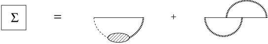
FIG. 5.: The electron self-energy operator with screening and hole-particle interaction included.

FIG. 6.: Lowest-order correlation corrections to the PNC E1 transition amplitude. Dashed line is the E1 field; cross is the nuclear weak field.

FIG. 7.: Small corrections to the PNC E1 transition amplitude: external field inside the correlation potential. In diagrams (a) the weak interaction is inside the correlation potential ($\delta\hat{\Sigma}$ denotes the change in $\hat{\Sigma}$ due to the weak interaction); this is known as the weak correlation potential. Diagrams (b) represent structural radiation (photon field inside the correlation potential).

FIG. 8.: High-frequency contribution to radiative corrections. Diagram (a) corresponds to the Uehling potential. Diagram (b) is the vertex correction. The single solid line represents the bound electron; the double line is the free electron; the Coulomb interaction is denoted by the dashed line; and the filled circle denotes the nucleus.