Parton Distribution Functions suitable for Monte-Carlo event generators

Abstract:

In the usual factorization theorems, which give predictions only for inclusive cross sections, there is considerable freedom in the choice of the scheme to define the parton distribution functions. These theorems do not directly apply to Monte-Carlo event generators, and more general factorization theorems which give predictions for fully exclusive cross sections are needed. It has been shown that appropriate parton distribution functions are uniquely defined by the showering algorithm. In this paper, we present results of calculations of the Monte-Carlo parton distribution functions in terms of the commonly used $\overline{\rm MS}$ parton distribution functions. At small $x$ the differences are large, which demonstrates the importance of using the correct parton distribution functions in an event generator rather than $\overline{\rm MS}$ parton distribution functions. We present some simple approximations that enable an understanding of the sizes of the results to be obtained.

1 Introduction

The standard factorization theorems [1] of QCD only give predictions for inclusive cross sections. In Monte-Carlo (MC) event generators we generate complete events and implement QCD predictions for the detailed structure of the final state, therefore it is important to get both the inclusive cross section and the exclusive cross sections right.

For inclusive cross sections, there is freedom in choosing the factorization scheme that defines the parton distribution functions (pdfs). But one of us has shown [2] that this is not the case in MC event generators; the specific showering algorithm used in a particular event generator entails a particular definition of the pdfs that should be used in the event generator. In this paper we first expand these arguments, showing how they are related to the requirement of obtaining correct exclusive cross sections.

We then present and analyze the results of calculations for pdfs that are appropriate to the algorithm of Bengtsson, Sjöstrand and van Zijl [3], as is used, for example, in the event generators PYTHIA and RAPGAP. In order to reach the next-to-leading order (NLO) accuracy in both the inclusive and the exclusive cross sections, it is important to use the correct pdfs and the correspondingly determined NLO hard scattering coefficients. As an example, we show that in the DIS $F_{2}$ calculation, using $\overline{\rm MS}$ pdfs instead of the correct ones for the specific event generator introduces an error of roughly $40\%$ at small $x$. This can, of course, substantially affect the phenomenology.

2 Factorization Schemes and Parton Distribution Functions in Monte-Carlo event generators

2.1 Factorization theorem and Monte-Carlo event generators

The factorization theorem states that appropriate inclusive cross sections with a large transverse momentum $Q$ are given [1] (to the leading power in $Q$) by a hard scattering coefficient convoluted with pdfs. Each hard scattering coefficient is infrared safe, calculable in perturbation theory and independent of the external hadron. The pdfs contain all the infrared sensitivity of the original cross section, they are external-hadron specific and are independent of the particular hard scattering process.

For inclusive cross sections, it is well known that there is some freedom in choosing the prescription by which the pdfs are defined. A set of rules that makes the choices is called a ‘factorization scheme’. Such a scheme both defines the pdfs and implies a rule for unambiguously calculating the hard scattering coefficients.

It might be concluded that this also applies to the hard scattering coefficients in an MC event generator. As shown by one of us [2], this is not in fact the case, and we will now review the reasoning.

An MC event generator calculates the exclusive components of the cross section, by using a combination of perturbatively calculated quantities for the larger scales and suitable modeling for the nonperturbative physics. The perturbative part consists of hard-scattering coefficients and evolution kernels. For the idea of computing NLO (and even higher order) corrections to make practical sense, the perturbative expansions of the hard scattering coefficients and the evolution kernels must be free of logarithms of large ratios of kinematic variables.

Figure 1: Two-parton correlation function used in definition of parton distribution function.

Since the cross section being computed is exclusive rather than inclusive, the reasoning leading to the factorization theorem for inclusive processes does not directly apply, and more general arguments are mandatory [2, 6]. Now a pdf $f_{i}(x)$ is essentially the number density of partons of flavor $i$ and fractional longitudinal momentum $x$ with an integral over transverse momentum and virtuality. An examination [2] of the derivation of the event generator algorithms shows that the form of this integral and its cutoff at large transverse momentum and virtuality are determined by the showering algorithm. For example, if the Bengtsson-Sjöstrand algorithm of Ref. [3] is used for the kinematics of the initial-state parton, then the pdf is

$$f_{i}(x)=\int d^{4}k\,\delta(x-k\cdot(k+q)/p\cdot q)\,\theta(Q^{2}-|k^{2}|)\,L(k,p),$$ (1)

where $L(k,p)$ is a two-particle correlation function of two partons in the target hadron, Fig. 1. The delta function gives the definition of the longitudinal fractional momentum variable in the algorithm, and the theta function implements the upper cutoff on virtuality. Some details concerning gauge invariance have not been precisely specified, but for our purposes this will not matter. In any case the definition is different from the $\overline{\rm MS}$ definition, and the specification of the showering algorithm implies a specific prescription for defining the pdfs, without any further choice.

In an event generator, the definitions of the parton kinematics in an initial-state shower are phenomenologically manifested in the kinematics of the hadronic final state. Hence if the parton kinematics are mismatched between the parton-shower algorithm and the definition of the pdf, the calculation of the final state is incorrect. This contrasts with the calculation of an inclusive cross section, where the relevant part of the final state is summed over; all that matters in an inclusive cross section is that given the kinematics for the struck parton a final state is generated with probability unity.

As usual, at lowest order it is legitimate to approximate the pdfs in the correct scheme by those in some other conveniently chosen scheme (e.g., $\overline{\rm MS}$). This is because the error caused by the incorrect pdf is of the same order as the error caused by the unimplemented NLO correction in the hard scattering. But beyond LO, this is not an appropriate approximation.

The methods of, for example, Pötter [5], suggest that the scheme for the pdfs can be chosen at will, with the scheme dependence of the pdfs being compensated for in the computation of the hard scattering. This reasoning appears to be incorrect. It starts from the assertion that the cross section is given by (‘bare’) pdfs convoluted with on-shell partonic matrix elements computed without any subtractions. Although this statement is often repeated in the literature, we know of no proof. Indeed it is a clearly unphysical statement, since in the real world of QCD partons are never on-shell. Moreover it is not necessary [7] for a correct proof of factorization. The incorrect starting assumption is particularly inappropriate for work with an event generator, where one explicitly treats the showering of partons that have much lower virtuality than that largest scale in the process. Furthermore, as we stated above, the standard factorization theorem and its derivation are not sufficient by themselves to derive an algorithm for parton showering, at NLO accuracy.

Moreover, the method of Pötter results in the real-emission part of the NLO hard scattering being obtained from unsubtracted partonic scattering graphs integrated down to a small cutoff $s_{\rm min}$. Real emission at NLO below the cutoff is assigned to the same parton configuration as the LO term; for this to be a useful approximation, $s_{\rm min}$ must be substantially smaller than the primary scale $Q^{2}$ of the hard scattering. This immediately implies that there is a double logarithm of the ratio $s_{\rm min}/Q^{2}$ in the integrated hard scattering coefficient. Since there will be corresponding logarithms in higher orders, this implies that the NLO hard scattering in this method is an inappropriate way of truncating a perturbation expansion.

Similar remarks apply to other proposals along similar lines, for example that of Dobbs [4].

2.2 Pdfs in MC event generators

In [2], a subtraction method was introduced to consistently take into account the LO and the NLO contributions for DIS in PYTHIA. Two different algorithms were discussed and formulas for the appropriate pdfs in terms of $\overline{\rm MS}$ pdfs were derived at the level of gluon-induced NLO terms. The gluon-induced term is particularly important because of the large size of the gluon distribution functions at small $x$. The algorithms are the standard Bengtsson-Sjöstrand algorithm [3] and a modified algorithm of Collins [2] which has improved kinematic properties. We label these algorithms “BS” and “JCC”.

In this section we review the derivation, which is made by comparing calculations of the contribution of quark $a$ to $F_{2}$ in the $\overline{\rm MS}$ scheme with the corresponding calculation in each of the event-generator algorithms:

$$F_{2}^{a}(x,Q^{2}) = xf_{a}^{\rm(\overline{\rm MS})}(x,\mu^{2})$$ (4)

$$+\frac{\alpha_{s}(\mu^{2})}{2\pi}\int_{x}^{1}d\xi\frac{x}{\xi}f^{(\overline{\rm MS})}_{g}(\xi,\mu^{2})\left[P(z)\ln\frac{Q^{2}(1-z)}{\mu^{2}z}-\frac{1}{2}+4z(1-z)\right]$$

$$+\mbox{ NLO quark terms}+O(\alpha_{s}^{2})$$

$$= xf^{\rm BS}_{a}(x,Q^{2})+\frac{\alpha_{s}(Q^{2})}{2\pi}\int_{x}^{1}d\xi\int_{-1}^{1}d\cos\theta\frac{x}{\xi}f_{g}(\xi,Q^{2})\times$$

$$~{}~{}\times\frac{1}{1-\cos\theta}\left\{\left[P(z)-C(-\hat{t})\frac{f_{a}(x)}{f_{a}(x_{1})}P\left(\frac{x_{1}}{\xi}\right)\right]-\frac{1}{4}+\frac{3}{2}z(1-z)\right\}$$

$$+\mbox{ NLO quark terms}+O(\alpha_{s}^{2})$$

$$= xf_{a}^{\rm JCC}(x,Q^{2})$$

$$+\frac{\alpha_{s}(Q^{2})}{2\pi}\int_{x}^{1}d\xi\frac{x}{\xi}f_{g}(\xi,Q^{2})\left[P(z)\ln 1/z-\frac{1}{2}+3z(1-z)\right]$$

$$+\mbox{ NLO quark terms}+O(\alpha_{s}^{2}).$$

Here $z=x/\xi$ while $P(z)=\frac{1}{2}[z^{2}+(1-z)^{2}]$ is the splitting kernel for gluon $\to$ quark-antiquark pair. In the formula for the BS algorithm, $x_{1}=x-\frac{1}{2}\xi(1-\cos\theta)$ and $-\hat{t}=Q^{2}(1-\cos\theta)\xi/2x$, while $C(-\hat{t})=\theta(Q^{2}+\hat{t})$ is the cutoff function for the showering.

We define $F_{2,{\rm\overline{\rm MS}}}^{\rm LO}$, $F_{2,{\rm BS}}^{\rm LO}$ and $F_{2,{\rm JCC}}^{\rm LO}$ to be the first terms on the right of each of Eqs. (4), (4) and (4) respectively. Similarly the second terms are called $F_{2,{\rm\overline{\rm MS}}}^{\rm NLO}$, $F_{2,{\rm BS}}^{\rm NLO}$ and $F_{2,{\rm JCC}}^{\rm NLO}$, respectively.

Formulas follow immediately [2, 8] for the quark distribution function in the BS scheme and the JCC scheme in terms of those in the $\overline{\rm MS}$ scheme:

$$xf^{\rm JCC}_{a}(x,\mu^{2}) = xf^{(\overline{\rm MS})}_{a}(x,\mu^{2})$$

$$+\frac{\alpha_{s}(\mu^{2})}{2\pi}\int_{x}^{1}d\xi\frac{x}{\xi}f^{(\overline{\rm MS})}_{g}(\xi,\mu^{2})\left[P(z)\ln(1-z)+z(1-z)\right]$$

$$+\mbox{ NLO quark terms}+O(\alpha_{s}^{2})$$

$$= xf^{(\overline{\rm MS})}_{a}(x,\mu^{2})+F_{2,{\rm\overline{\rm MS}}}^{\rm NLO}-F_{2,{\rm JCC}}^{\rm NLO}+\mbox{ NLO quark terms}+O(\alpha_{s}^{2}).$$

$$xf^{\rm BS}_{a}(x,\mu^{2}) = xf^{(\overline{\rm MS})}_{a}(x,\mu^{2})$$

$$+\frac{\alpha_{s}(\mu^{2})}{2\pi}\int_{x}^{1}d\xi\frac{x}{\xi}f^{(\overline{\rm MS})}_{g}(\xi,\mu^{2})\Bigg{\{}P(z)\ln\frac{1-z}{z}+z(1-z)$$

$$~{}~{}~{}\left.-\int_{-1}^{1}\frac{d\cos\theta}{1-\cos\theta}\left[P(z)-C(-\hat{t})\frac{f_{a}^{\rm BS}(x)}{f_{a}^{\rm BS}(x_{1})}P\left(\frac{x_{1}}{\xi}\right)\right]\right\}$$

$$+\mbox{ NLO quark terms}+O(\alpha_{s}^{2}),$$

$$= xf^{(\overline{\rm MS})}_{a}(x,\mu^{2})+F_{2,{\rm\overline{\rm MS}}}^{\rm NLO}-F_{2,{\rm BS}}^{\rm NLO}+\mbox{ NLO quark terms}+O(\alpha_{s}^{2}).$$

Note that Eq. (2.2) is a nonlinear equation in terms of $f_{a}^{\rm BS}$; this arises from the particular treatment of parton kinematics in the BS algorithm. When we calculate the numerical value of $f_{a}^{\rm BS}$, we will use $f_{a}^{\rm\overline{\rm MS}}$ in the integrand. We will justify this simplification in Sec. 2.4.

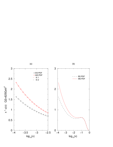
Figure 2: The left-hand graph gives the $u$-quark distribution at small $x$ at $Q^{2}=625\,{\rm GeV}^{2}$. The lines are simple power law fits to the curves: $xu(x)=0.135x^{-0.32}$ and $xu(x)=0.14x^{-0.27}$ for the upper ($\overline{\rm MS}$) and lower (BS scheme) curves. The inset gives the pdf at all $x$.

We have performed numerical calculations of the quark densities. Our code is based on earlier work by Sabine Schilling [9]. We have made the code available at [10]. Some results are shown in Fig. 2, which gives the $u$ quark distribution function in the $\overline{\rm MS}$ and BS schemes at $Q^{2}=625\,{\rm GeV}^{2}$, with the $\overline{\rm MS}$ density being that of CTEQ5 [11]. This figure clearly shows a large difference between the BS pdf and the $\overline{\rm MS}$ pdf at small $x$. The curves for the $d$-quark distribution function are quite similar, so we do not show them. In Secs. 2.3 and 2.4, we will analyze the scheme dependence of the pdfs in more detail.

If we use $\overline{\rm MS}$ pdfs rather than the ones appropriate to the BS algorithm of the event generator, the exclusive cross section will be in error by $\sim 40\%$ at small $x$, although it is possible to get the correct inclusive cross section, with the use of the well-known NLO correction in this scheme. As we will explain, this correction is unusually small, so that good results can be obtained for the inclusive cross section, i.e., for $F_{2}$, even without the use of the NLO correction, if the $\overline{\rm MS}$ scheme is used.

We conclude that, while $\overline{\rm MS}$ pdfs are well-defined quantities and are appropriately used in calculations of inclusive cross sections, they are not suitable for use in MC event generators where the fully exclusive cross sections are our main concern.

For the same reason, the pdfs used in [4, 5] which are essentially $\overline{\rm MS}$ pdfs with “scheme-dependence” corrections, are not appropriate pdfs to use in the event generators.

2.3 The NLO contributions to $F_{2}$

In this section we investigate the relative size of the NLO and LO contributions to $F_{2}$, with the aid of some useful approximations, and we show that the substantial differences between the schemes are to be expected, because of the large size of the gluon distribution function. A surprising result is that the NLO corrections to $F_{2}$ in the $\overline{\rm MS}$ scheme are unusually small, as the result of special cancellations.

From Eqs. (4), (4) and (4), the relative sizes of the NLO terms can be estimated as follows:

$$\frac{F_{2}^{\rm NLO}}{F_{2}^{\rm LO}} = \frac{\alpha_{s}}{2\pi}\int_{x}^{1}d\xi\frac{x}{\xi}f_{g}(\xi)O(1)$$ (7)

$$\sim \frac{\alpha_{s}}{2\pi}f_{g}(2x)/f_{a}(x).$$

This estimate is appropriate to the small $x$ region. We have first observed that each integral contains a factor $\alpha_{s}/2\pi$, a factor of the gluon distribution function and a factor of order unity. At small $x$, the important values of $\xi$ range from $x$ to a modest factor times $x$, so that we set the argument of the gluon distribution function to $2x$, as an estimate of the typical value of $\xi$.

The ratio of NLO to LO would generally be at most of order $\alpha_{s}/2\pi$, which is appropriate for a generic NLO correction, were it not that the gluon distribution function is large at small $x$. Clearly, there should be an enhancement of the NLO contribution, and the above formula gives the expected size.

Fig. 3 displays the numerical value of the ratio of the NLO and the LO terms in $F_{2}$ for different factorization schemes at $Q^{2}=33.8\,{\rm GeV}^{2}$, in the case of the $u$ quark. The figure also show the results for the simple estimate (7). Results for other flavors would be similar.

For the BS scheme, the large gluon distribution function at small $x$ does indeed give a substantial effect: the NLO contribution is close to $100\%$ of the LO contribution at $x=10^{-4}$. The effect is much smaller at large $x$. The plot of the simple estimate (7) shows that this behavior is completely expected. The accuracy of the approximation is an accident, but the overall size is not.

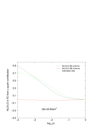
Figure 3: Ratio of the NLO and LO terms in $F_{2}$ from u quark contribution for different factorization schemes. We also show the simple estimate $\frac{\alpha_{s}}{2\pi}\frac{f_{g}(2x)}{f_{a}(x)}$ Eq. (7).

For the commonly used $\overline{\rm MS}$ scheme, the NLO corrections are rather small for all $x$. In view of the expected size of generic NLO corrections, we should regard the small size of the correction in $\overline{\rm MS}$ as an accident that is useful for phenomenology rather than as a fundamental expectation. The cancellation is associated with the particular sizes of the positive and negative terms in the second line of Eq. (4).

To understand this cancellation better, it is convenient to perform a slightly different approximation where we replace the pdfs by power laws. At small $x$, the gluon distribution function $f_{g}(x)$ is roughly $C/x^{q}$ and the quark distribution function $f_{a}(x)$ is roughly $C^{\prime}/x^{r}$. This gives the following approximations for each of the $F_{2}^{\rm NLO}$s:

$$F_{2,{\rm\overline{\rm MS}}}^{\rm NLO}(x,Q^{2}) \approx \frac{\alpha_{s}(Q^{2})}{2\pi}Cx^{1-q}\int_{0}^{1}dzz^{q-1}\left[P(z)\ln\frac{1}{z}+4z(1-z)\right]$$ (8)

$$-\frac{\alpha_{s}(Q^{2})}{2\pi}Cx^{1-q}\int_{0}^{1}dzz^{q-1}\left[P(z)\ln\frac{1}{1-z}+\frac{1}{2}\right],$$

$$F_{2,{\rm BS}}^{\rm NLO}(x,Q^{2}) \approx \frac{\alpha_{s}(Q^{2})}{2\pi}Cx^{1-q}\int_{0}^{1}dzz^{q-1}\Bigg{\{}P(z)\ln\frac{1}{z}-\frac{1}{2}+3z(1-z)$$ (9)

$$+\int_{O}^{2z}dy\left[P(z)\frac{1-(1-\frac{y}{2z})^{r}}{y}-\left(1-\frac{y}{2z}\right)^{r}\left(\frac{1}{4}y-z+\frac{1}{2}\right)\right]\Bigg{\}}$$

$$\approx \frac{\alpha_{s}(Q^{2})}{2\pi}Cx^{1-q}\int_{0}^{1}dzz^{q-1}\left[P(z)\ln\frac{1}{z}+\frac{3}{2}z(1-z)+\frac{1}{3}z^{2}\right],$$

$$F_{2,{\rm JCC}}^{\rm NLO}(x,Q^{2}) \approx \frac{\alpha_{s}(Q^{2})}{2\pi}Cx^{1-q}\int_{0}^{1}dzz^{q-1}\left[P(z)\ln\frac{1}{z}+3z(1-z)-\frac{1}{2}\right].$$ (10)

In each case, the lower limit of the $z$ integral can be set to zero when $x$ is small, and we therefore have a simple power of $x$ times a fixed integral over $z$.

The integrals of $z$ in the above equations are basically all of $O(1)$. The exponent $q$ is about $1.2\sim 1.4$ for the gluon distribution function. The exponent $r$ for the quark distribution is close to 1 and less than $q$. Therefore, the NLO corrections will be enhanced at small $x$. However there are negative terms in the $\overline{\rm MS}$ integral which results in a cancellation. There is a weaker cancellation in the integral for the JCC scheme, but there is no cancellation in the integral for the BS scheme.

2.4 Accuracy of nonlinear term in BS pdfs

The BS quark distribution function is related to the $\overline{\rm MS}$ distribution function by the nonlinear integral shown in Eq. (2.2). As is normal, we replace the BS pdfs on the right-hand side by the $\overline{\rm MS}$ pdfs, so that we get a formula involving $\overline{\rm MS}$ pdfs only. Generally this is the normal procedure since the change involves an effect of relative order $\alpha_{s}$ in an NLO term. In transformations that are linear in the pdfs, this is quite sensible: All the errors are handled by the uncalculated terms of yet higher order. However, this is more delicate for the nonlinear formula, particularly given that the quark distribution functions have large corrections. A linear formula, as for the JCC scheme, only needs the gluon distribution function, but our nonlinear formula also involves the quark distribution functions.

In this section we will show that this issue does not in fact affect the accuracy of our calculations, since the right-hand side of Eq. (2.2) only involves a ratio of quark distribution functions; the ratio of BS quark distribution functions, $f_{a}^{\rm BS}(x)/f_{a}^{\rm BS}(x_{1})$, is equal to the ratio of the $\overline{\rm MS}$ distribution functions to a good approximation.

Our demonstration is semi-analytic, so that we can see that the result is robust against changes in the pdfs.

In Fig. 2, we fit the small $x$ pdfs with $y=Ax^{B}$. The exponent $B$ of $x$ depends on $Q^{2}$, but the difference of exponent between the BS scheme and the $\overline{\rm MS}$ scheme is roughly the same for all $Q^{2}$ and approximately equal to 0.05.

The error introduced by the replacement of the BS quark distribution functions by the $\overline{\rm MS}$ distribution functions on the right-hand side of Eq. (2.2) is then

$$\delta \equiv \frac{\alpha_{s}(Q^{2})}{2\pi}\int_{0}^{1}dz\frac{x}{z}f_{g}\left(\frac{x}{z}\right)\int_{1-2z}^{1}\frac{d\cos\theta}{1-\cos\theta}P(z_{1})\left[\frac{f_{a}^{\rm\overline{\rm MS}}(x)}{f_{a}^{\rm\overline{\rm MS}}(x_{1})}-\frac{f_{a}^{\rm BS}(x)}{f_{a}^{\rm BS}(x_{1})}\right],$$ (11)

where $z_{1}=z-(1-\cos\theta)/2$.

The error $\delta$ is the largest in small $x$ region because of the large difference between the $\overline{\rm MS}$ pdfs and the BS pdfs. When $\cos\theta\to 1-2z$, $x_{1}\to 0$, and then $f_{a}(x)/f_{a}(x_{1})\to 0$, therefore $\delta$ is very small. When $\cos\theta\to 1$, $x_{1}\sim x$, we have

$$\frac{f_{a}(x)}{f_{a}(x_{1})}\approx 1-\frac{\xi}{2}(1-\cos\theta)\frac{f^{\prime}_{a}(x)}{f_{a}(x)}$$ (12)

and $f_{a}^{\overline{\rm MS}}(x)\sim A_{1}/x^{1.32}$, $f_{a}^{\rm BS}(x)\sim A_{2}/x^{1.27}$.

We can see that $\delta$ depends on the pdfs through their difference in exponents of $x$, rather than on the actual value of pdfs. Given the exponents of the BS pdf and the $\overline{\rm MS}$ pdf, we have,

$$\delta\approx\frac{\alpha_{s}}{2\pi}\int_{0}^{1}dz\frac{x}{z}f_{g}(\frac{x}{z})P(z)/z\times 0.025$$ (13)

which is less than $5\%$ of $F_{2,{\rm BS}}^{\rm NLO}$. Therefore, our simplification is valid up to NLO accuracy.

3 Conclusion

We explained that the pdfs in MC event generators are determined by the showering algorithm, and cannot be freely chosen, unlike the case for pdfs used in inclusive calculations. The rules for calculating the hard-scattering coefficients at higher orders are then unambiguously defined. We then presented some numerical calculations of the quark distribution functions to be used with the BS algorithm. At small $x$ the corrections are large, so that the commonly used $\overline{\rm MS}$ pdfs are inappropriate for use in event generators. We used some simple approximations to understand the size of the corrections and to show that the large correction is to be expected.

The code for the MC-specific pdfs is available at [10].

Note Added

Early papers on HERWIG, for example the paper of Marchesini and Webber [12], also mentioned the idea that the showering algorithm entails a particular definition of the pdfs, with cutoffs on parton kinematics that correspond to cutoffs in the showering. However, since the event generator was only implemented at leading order, the need for modified pdfs was not emphasized in Ref. [12]; it was sufficient to use unmodified pdfs from standard fits.

We thank the referee for bringing this work to our attention.

References

- [1] R. Brock et al. [CTEQ Collaboration], Rev. Mod. Phys. 67 (1995) 157.
- [2] J. Collins, J. High Energy Phys. 05 (2000) 004, hep-ph/0001040.
-
[3]
T. Sjöstrand,
Phys. Lett. B 157 (1985) 321
M. Bengtsson and T. Sjöstrand, Z. Physik C 37 (1988) 465. - [4] M. Dobbs, hep-ph/0111234.
-
[5]
B. Pötter,
Phys. Rev. D 63 (2001) 114017,
hep-ph/0007172.
B. Pötter and T. Schörner, Phys. Lett. B 517 (2001) 86, hep-ph/0104261. - [6] J. Collins, hep-ph/0110113, to be published in Phys. Rev. D.
- [7] J.C. Collins, D.E. Soper and G. Sterman, “Factorization Of Hard Processes In QCD,” in “Perturbative QCD” (A.H. Mueller, ed.) (World Scientific, Singapore, 1989), and references therein.
- [8] Y. Chen, J. Collins and N. Tkachuk, J. High Energy Phys. 06 (2001) 015, hep-ph/0105291.
- [9] S. Schilling, Diploma thesis DESY–THESIS–2000–040, http://www-library.desy.de/cgi-bin/showprep.pl?desy-thesis00-040.
- [10] Code used to calculate the MC-specific parton densities is available at http://www.phys.psu.edu/~cteq/collins/mc-pdf/.
- [11] H.L. Lai et al. [CTEQ Collaboration], Eur. Phys. J. C 12 (2000) 375, hep-ph/9903282.
- [12] G. Marchesini and B.R. Webber, Nucl. Phys. B 310 (1988) 461.