Realistic extremely flat scalar potential in 3-3-1 models

Abstract

We show that in 3-3-1 models it is possible to implement an extremely flat scalar potential, i.e., a zero contribution to the cosmological constant, and still having realistic values for the masses of the scalar Higgs fields. Besides, when loop corrections are considered they impose constraints over heavy particles masses (exotic quarks and extra vector bosons) which are present in the model. A crucial ingredient in 3-3-1 models is the existence of trilinear terms in the scalar potential. We also consider the two-Higgs doublets extension of the standard model with and without supersymmetry.

I Introduction

The cosmological constant $\Lambda$ was initially postulated by Einstein who included by hand the term $\Lambda g_{\mu\nu}$ in his gravitational theory in order to obtain a static Universe solution. In subsequent works the meaning of this term was clarified and it was shown that it is linked with the vacuum energy density. The Einstein’s field equations with the $\Lambda$-term are

$$R_{\mu\nu}-\frac{R}{2}g_{\mu\nu}-\Lambda g_{\mu\nu}=8\pi GT_{\mu\nu},$$ (1)

where $R_{\mu\nu}$ is the Ricci tensor, $g_{\mu\nu}$ is the metric tensor and $R$ represents the curvature scalar of the space-time and $T_{\mu\nu}$ is the energy momentum tensor; $G$ is the constant of gravitation. The so-called “cosmological constant problem” [1] consists in the fact that the values of the vacuum energy densities related to quantum field energy scales, for instance, quark condensates $\langle q\bar{q}\rangle$, $\Lambda_{\rm QCD}$ and to the Planck scale $\Lambda_{\rm Planck}$, are several orders of magnitude larger than the values suggested by the astronomical observations (see below).

In the context of classical general relativity we can always omit the $\Lambda$-term in the Lagrangian. On the other hand, in quantum field theory only energy differences are measured, so we can always redefine the vacuum energy in such a way that it always corresponds to zero energy. However, since gravitation is sensible to the absolute value of the energy, through distortions in the space-time, all matter and energy forms couple to gravitation. It means that the metric $g_{\mu\nu}$ can be coupled as an external field to the bare action of a quantum field theory playing the role of a source for the energy-momentum operator [2]. Therefore we cannot avoid the problem when both gravitational phenomena and quantum field theory are taken into account, because in this situation it is not allowed to redefine the vacuum energy [3, 4, 5].

Until the end of the nineties, astronomical data were able to give for the value of $|\Lambda_{\rm obs}|$ only an upper bound. Because of the smallness of the bound, compared with the theoretically expected values, many attempts were made in order to find models in which the total cosmological constant was exactly zero [6]. None of these attempts, however, is based on some fundamental theory and at present only considerations based on the anthropic principle suggest a route towards the response to the cosmological constant question. However, although these considerations receive support from the inflationary cosmological models, they do not have yet experimental basis [1, 7, 8]. The effort spent to solve this (still open) problem is justified since the geometry and the evolution of the Universe are closely related to it [4, 8, 9]. Therefore, advances in this problem may lead us to a better understanding of some of the crucial problems in both cosmology and elementary particle physics. In the latter, this problem is related to another not well understood question: the mechanism of mass generation via the spontaneous symmetry breaking (SSB), through scalar Higgs fields with a non-zero vacuum expectation value (VEV). That mechanism also implies a new large contribution to the cosmological term in the Einstein’s equations [10]. We named this the “electroweak cosmological constant” (ECC) in order to left clear the difference with other quantum field contributions to the cosmological constant as those mentioned before.

Independently of these theoretical issues, recent astronomical observations [11, 12, 13, 14] strongly suggest a nonzero and positive $\Lambda$. This result comes from observations of Type Ia supernova [11], gravitational lensing frequencies for quasars [12] and harmonics of cosmic background radiation (CBR) anisotropies [13]. These astronomical data gives $0.6<\Omega_{\Lambda}<0.8$, where $\Omega_{\Lambda}=\Lambda/3H^{2}_{0}$ is the $\Lambda$ density in units of critical universe mass density, with $H_{0}=71$ km s^-1Mpc^-1, (1 s = $1.52\times 10^{24}$ GeV^-1 and 1 pc = $3.086\times 10^{16}$ m [15]). Assuming $\Omega_{\Lambda}=0.7$ we have

$$\Lambda_{\rm obs}=4.8\times 10^{-84}\;{\rm GeV}^{2}\quad({\rm or}\quad\Lambda_{\rm obs}G\approx 10^{-122}),$$ (2)

where we have used $G=6.71\times 10^{-39}$ GeV^-2 and $\hbar=c=1$.

In this work we are interested only in the contributions of the scalar Higgs sector to the vacuum energy density. Models with the scalar fields, denoted collectively by $\Phi$, with the respective scalar potential $V\left(\Phi\right)$, have a part in the energy momentum tensor given by

$$T_{\mu\nu}=\partial_{\mu}\Phi\partial_{\nu}\Phi-g_{\mu\nu}\left(\frac{1}{2}g^{\alpha\beta}\partial_{\alpha}\Phi\partial_{\beta}\Phi-V(\Phi)\right).$$ (3)

The vacuum part in $T_{\mu\nu}$ is gotten when $\partial_{\mu}\Phi=0$ so that, denoting the VEVs of the neutral component of the Higgs fields collectively as $\Phi$ by $\langle\phi\rangle$, we have that the vacuum energy momentum tensor is

$$T^{\rm vac}_{\mu\nu}=g_{\mu\nu}V\left(\langle\phi\rangle\right)=g_{\mu\nu}\rho_{\Lambda_{W}}\equiv g_{\mu\nu}\frac{\Lambda_{W}}{8\pi G},$$ (4)

where $\rho_{\Lambda_{W}}$ is the vacuum energy density. We can write the purely electroweak contribution to the cosmological constant $\Lambda_{W}=8\pi GV(\langle\phi\rangle)$.

Hence, in addition to the intrinsic cosmological constant in the Einstein equation, $\Lambda$ in Eq. (1), there is a contribution to the vacuum energy coming from SSB sector, so the observed or effective cosmological constant is [5]

$$\Lambda_{\rm eff}=\Lambda-8\pi G|V(\langle\phi\rangle)|.$$ (5)

It is $\Lambda_{\rm eff}$ which should coincide with $\Lambda_{\rm obs}$ i.e., $\Lambda_{\rm eff}\approx\Lambda_{\rm obs}$, and this can be obtained if

$$\Lambda_{\rm eff}\approx\Lambda_{\rm obs}\quad(a);\quad{\rm or}\quad\Lambda\approx\Lambda_{\rm obs},\quad 8\pi GV(\langle\phi\rangle)=0\quad(b).$$ (6)

Eq. (6a) implies that there exist a fine tuning between two parameters which are different in the sense that $\Lambda$ does not depend on the matter fields while $8\pi GV(\langle\phi\rangle)$ does. We may wonder ourselves how this fine tuning is possible between terms which so different physical origin. It will be more natural that $\Lambda\approx\Lambda_{\rm obs}$ while $8\pi GV(\langle\phi\rangle)=0$. The first possibility, Eq. (6a), can be implemented in any electroweak model and for this reason it is not so much interesting as a solution to the electroweak cosmological constant problem. On the other hand, it is not clear at all in which kind of models (if any) the case in Eq. (6b) is realized. In other words, in general we will look for an interval for the possible values for $\Lambda$

$$\Lambda_{\rm obs}+8\pi G|V(\langle\phi\rangle)_{m}|\leq\Lambda\leq\Lambda_{\rm obs}+8\pi G|V(\langle\phi\rangle)_{M}|$$ (7)

in which $|V(\langle\phi\rangle)_{M}|$ ($|V(\langle\phi\rangle)_{m}|$) is the largest (smallest) value of $|V(\langle\phi\rangle)|$. It is well known, and we will review this in the next section, that in the standard model $|V(\langle\phi\rangle)_{M}|=|V(\langle\phi\rangle)_{m}|\equiv|V(\langle\phi\rangle)|$ and for this reason only the fine tuning $\Lambda=\Lambda_{\rm obs}+8\pi G|V(\langle\phi\rangle)|$ is allowed and $\Lambda_{\rm eff}\approx\Lambda_{\rm obs}$ as in Eq. (6a).

Here a remark is in order. It is always possible to add an arbitrary constant $V_{0}\equiv V(\Phi=0)$ to the scalar potential, in such a way that $V(\langle\phi\rangle)\to V(\langle\phi\rangle)+V_{0}$ in Eq. (5). We may consider $V_{0}$ as a bare cosmological constant in Einstein equation as in Eq. (1). This follows because if $L_{\rm matter}$ denotes the matter Lagrangian, which includes the scalar potential $V(\Phi)$, we can also use $L_{\rm matter}^{\prime}=L_{\rm matter}-V_{0}$ instead of just $L_{\rm matter}$. Both Lagrangians give the same equation of motion for the matter, moreover, $V_{0}$ is a model independent parameter in the sense that it does not depend on the fields of the model and it is the same for all electroweak models. In fact, $V_{0}$ (or $\Lambda$) does not depend on the state of the Universe. Hence, it is possible to identify $\Lambda$ with $8\pi GV_{0}$ i.e., $\Lambda\equiv 8\pi GV_{0}$ or, more properly that $\Lambda+8\pi GV_{0}\to\Lambda^{\prime}$ and just omit the prime.

We are also not assuming any form of exotic dark matter inducing a highly negative pressure [16]. Hence, we will neglect other contributions to the vacuum energy density and consider only the contributions of the Higgs scalars. It means that we will compare, under the same assumptions, only the electroweak contributions to the vacuum energy density in several electroweak models.

The outline of this paper is the following. In Sec. II we consider the cosmological constant coming from SSB in the context of the electroweak standard model. As it is known in that model a fine tuning, only among the parameters of the scalar potential, is not allowed since it would imply a rather light Higgs boson. Next, in Sec. III, we show that the troubles survives in the multi-Higgs extensions of the standard model with or without supersymmetry. In Sec. IV we analyze one of the so called 3-3-1 models, including 1-loop effective potential, in a version of the model with only three Higgs triplets [17]. We also, briefly, comment the case of the 3-3-1 model with a scalar sextet [18]. Our conclusions appear in the last section.

II The ECC in the standard model

To clarify our goal in this work let us consider the ECC problem in the context of the standard electroweak model. There the scalar potential is

$$V_{\rm SM}=\frac{1}{2}\left[\mu^{2}\Phi^{\dagger}\Phi+\frac{\lambda}{2}\left(\Phi^{\dagger}\Phi\right)^{2}\right],$$ (8)

where $\mu^{2}<0$ and $\lambda>0$ are parameters of the potential and $\Phi=\left(\begin{array}[]{cc}\phi^{+}&\phi^{0}\end{array}\right)^{T}$ is the only Higgs scalar doublet present in the model. The neutral component $\phi^{0}$ gets a non-zero VEV $v_{W}\approx 246$ GeV. When we take the potential at the minimum point we find

$$V_{\rm SM}(v_{W})=-\frac{\lambda}{4}\;v_{W}^{4}.$$ (9)

implying that $\Lambda_{W}=8\pi GV_{\rm SM}(v_{W})\approx-3.4\times 10^{-28}\;\lambda\;{\rm GeV}^{2}$, which is, independently of the minus sign, several order of magnitude larger than $\Lambda_{\rm obs}$ (see Eq. (2)) unless we impose that the constant of the scalar potential has an appropriate value: $\lambda=1.4\times 10^{-56}$. However, since the mass of the Higgs scalar is given by $m_{H}=\sqrt{2\lambda}\,v_{W}$, that value for $\lambda$ implies a rather light scalar $m_{H}\sim 10^{-22}m_{e}$, where $m_{e}$ is the electron mass [10]. A Higgs boson with mass $\lesssim 5$ GeV has been ruled out by a variety of arguments derived from rare decays, static properties like the magnetic moment of the muon, and nuclear physics [19]. So, in the SM we cannot use a fine-tuning among its parameters for obtaining a cosmological constant compatible with the observed value, and at the same time to obtain a scalar Higgs field with a mass of the order of 115.6 GeV [20]. In other words, in the standard model we have that $V_{\rm SM}(v_{W})=-2\lambda\times 10^{9}\,{\rm GeV}^{4}$. Since $V_{\rm obs}=\Lambda_{\rm obs}/8\pi G=2.8\times 10^{-47}\,{\rm GeV}^{4}$ it means that $|V_{\rm SM}(v_{W})/V_{\rm obs}|\approx\lambda\times 10^{56}$ and since from the experimental data we have that $\lambda\stackrel{{\scriptstyle>}}{{\sim}}0.13$, we see that only the case in Eq. (6a) is possible in this model.

From the phenomenological point of view this is not a fault of the (any) electroweak model. However, we may wonder ourselves if it is possible to built a model in which there is no a contribution to the cosmological constant coming from the SSB sector and having, at the same time, a realistic mass spectrum in the scalar sector.

III Multi-Higgs models

In this section we will consider two popular extension of the standard model: the two doublets, in Sec. III A, and the minimal supersymmetric standard model (MSSM), in Sec. III B.

A Two Higgs scalar non-supersymmetric model

In the two doublets non-supersymmetric extension of the standard model the Higgs scalars are $\Phi_{1}=\left(\begin{array}[]{cc}\phi_{1}^{+}&\phi^{0}_{1}\end{array}\right)^{T}$ and $\Phi_{2}=\left(\begin{array}[]{cc}\phi_{2}^{+}&\phi_{2}^{0}\end{array}\right)^{T}$ with the VEVs $\langle\phi_{1}^{0}\rangle=v_{1}/\sqrt{2}$ and $\langle\phi_{1}^{0}\rangle=v_{2}/\sqrt{2}$ and $v^{2}_{1}+v^{2}_{2}=v^{2}_{W}$. Its $CP$-conserving scalar potential is given by [19]

$$V_{\rm TD} = \mu_{1}^{2}\,\Phi_{1}^{\dagger}\Phi_{1}+\mu_{2}^{2}\,\Phi_{2}^{\dagger}\Phi_{2}+a_{1}\left(\Phi_{1}^{\dagger}\Phi_{1}\right)^{2}+a_{2}\left(\Phi_{2}^{\dagger}\Phi_{2}\right)^{2}+a_{3}\left(\Phi_{1}^{\dagger}\Phi_{1}\right)\left(\Phi_{2}^{\dagger}\Phi_{2}\right)$$ (10)

$$+ a_{4}(\Phi_{1}^{\dagger}\Phi_{2})(\Phi^{\dagger}_{2}\Phi_{1})+a_{5}\left[\left(\Phi_{1}^{\dagger}\Phi_{2}\right)^{2}+H.c.\right],$$ (11)

and we have assumed invariance under $\Phi_{2}\to-\Phi_{2}$ [21].

Thus, the vanishing of the linear terms in the neutral fields gives the constraints

$$-\mu_{1}^{2}=a_{1}v_{1}^{2}+\frac{1}{2}(a_{3}+a_{4}+2a_{5})v_{2}^{2},\qquad-\mu_{2}^{2}=a_{2}v_{2}^{2}+\frac{1}{2}(a_{3}+a_{4}+2a_{5})v_{1}^{2},$$ (12)

while the positivity of the Higgs bosons mass matrices implies

$$a_{1},a_{2}>0,\;\;a_{5}<0,\;\;(a_{3}+a_{4}+2a_{5})^{2}<4a_{1}a_{2},\;\;a_{4}+2a_{5}<0.$$ (13)

Next, using Eqs. (12) the minimum of the potential is

$$V_{\rm TD}({\rm min})\equiv V_{\rm TD}(v_{1},v_{2})=-\frac{1}{4}\,a_{1}v^{4}_{1}-\frac{1}{4}\,a_{2}v^{4}_{2}-\frac{1}{4}\,(a_{3}+a_{4}+2a_{5})v^{2}_{1}v^{2}_{2}.$$ (14)

It is easy to verify that a solution to the equation $V_{\rm TD}(v_{1},v_{2})=0$, that at the same time satisfies the constraints in Eq. (13), does not exist. Hence, in this model we have always a negative contribution to the vacuum energy. In fact, we can write Eq. (14) in terms of the masses of the neutral physical Higgs of the model $m_{H_{1,2}}$

$$V_{\rm TD}({\rm min})=-\frac{1}{16}\,\frac{1}{a_{1}+a_{2}-(a_{3}+a_{4}+2a_{5})}\,\frac{m^{2}_{H_{1}}m^{2}_{H_{2}}}{\tilde{v}^{2}_{1}(v^{2}_{W}-\tilde{v}^{2}_{1})}\cdot v^{4}_{W},$$ (15)

where $\tilde{v}_{1}$, is given by

$$\tilde{v}^{2}_{1}=\frac{1}{2}\,\frac{2a_{2}-(a-3+a_{4}+2a_{5})}{a_{1}+a_{2}-(a_{3}+a_{4}+2a_{5})}v^{2}_{W},$$ (16)

has been obtained from the condition $\partial V_{\rm TD}({\rm min})/\partial v_{1}=0$.

We see that in this two doublet extension of the SM $V_{\rm TD}({\rm min})_{M}\approx V_{\rm TD}({\rm min})_{m}\approx V_{\rm TD}({\rm min})$, and the interval allowed for $\Lambda$ in Eq. (7) is a rather small one i.e., in practice we have that like in the SM model $\Lambda\approx\Lambda_{\rm obs}+V_{\rm TD}({\rm min})$. Thus, as in the previous section the only fine tuning allowed is $\Lambda\stackrel{{\scriptstyle>}}{{\sim}}+10^{56}\Lambda_{\rm obs}$. Notice also from Eq. (15) that a vanishing contribution of the scalar potential to the cosmological constant implies also a zero mass neutral scalar. In this situation it is not worthing to calculate loop corrections to the scalar potential.

B Minimal supersymmetric standard model

The minimal supersymmetric model has also two scalar doublets, $H_{1}=(H^{0*}_{1},\,-H^{-}_{1})^{T}$ and $H_{2}=(H_{2}^{+},\,H_{2}^{0})^{T}$. The associated scalar potential is in this case [22, 23]

$$V_{\rm S} = m_{1}^{2}|H_{1}|^{2}+m_{2}^{2}|H_{2}|^{2}-m_{3}^{2}\left(\epsilon_{ij}H^{i}_{1}H^{j}_{2}+{\mbox{H. c.}}\right)+\frac{1}{8}\left[g^{2}\sum_{i}|H_{1}^{\dagger}\tau_{i}H_{1}+H_{2}^{\dagger}\tau_{i}H_{2}|^{2}\right.$$ (18)

$$\left.+g^{\prime 2}\left(|H_{1}|^{2}-|H_{2}|^{2}\right)^{2}\right],$$

where $m_{1}$, $m_{2}$ and $m_{3}$ are parameters with dimension of mass, $\tau_{i}$ $\left(i=1,2,3\right)$ are the Pauli matrices, $g^{\prime}=g\tan{\theta_{W}}$ and $g=2\sqrt{\sqrt{2}G_{F}}M_{W}$. As before we define the VEVs as $\langle H^{0}_{1}\rangle=v_{1}/\sqrt{2}$, $\langle H^{0}_{2}\rangle=v_{2}/\sqrt{2}$, with $v_{1}^{2}+v_{2}^{2}=v_{W}^{2}$, and the constraints equations are:

$$-m_{1}^{2} = \frac{1}{8v_{1}}\left[v_{1}\left(g^{2}+g^{\prime 2}\right)\left(v_{2}^{2}-v_{1}^{2}\right)+4m_{3}^{2}v_{2}\right],$$ (20)

$$-m_{2}^{2} = \frac{1}{8v_{2}}\left[v_{2}\left(g^{2}+g^{\prime 2}\right)\left(v_{1}^{2}-v_{2}^{2}\right)+4m_{3}^{2}v_{1}\right].$$ (21)

Therefore, taking the potential in the minimum we find

$$V_{\rm S}({\rm min})\equiv V_{\rm S}(v_{1},v_{2}) = -\frac{g^{2}}{32\cos^{2}\theta_{W}}\left(v_{1}^{2}-v_{2}^{2}\right)^{2},$$ (22)

$$= -\frac{v_{1}v_{2}}{8m^{2}_{3}}m^{2}_{H_{1}}m^{2}_{H_{2}}.$$ (23)

In the second line $m^{2}_{H_{1,2}}$ denote, like in the previous model, the mass square of the two physical neutral scalars of the model. The fine tuning $V_{\rm S}({\rm min})=0$ in Eq. (23), occurring apparently with $v_{1}=v_{2}$, is not possible since it implies that one of the neutral Higgs is massless, and we have a similar situation to the two previously considered cases i.e., the minimum of the potential is proportional to the mass(es) of the neutral Higgs scalar(s). On the other hand, the 1-loop corrections vanishes because of the supersymmetry. However, this occurs only in the early universe when $T>T_{\rm SUSY}$ and since we are now at $T<T_{\rm SUSY}$ this is not a desirable scenario. Anyway, the soft terms that have to be added to break the supersymmetry will induce non-zero contributions to $\Lambda_{W}$, at both tree and 1-loop level, which are also of the order of $|\Lambda_{W}|\stackrel{{\scriptstyle>}}{{\sim}}10^{56}\Lambda_{\rm obs}$, and this is the only possibility.

IV The cosmological constant in a 3-3-1 model

Another model that we will consider here is the three scalar triplet version of the 3-3-1 model [17]. In this kind of model the gauge symmetry $SU(3)_{C}\otimes SU(2)_{L}\otimes U(1)_{Y}$ of the standard model is extended to $SU(3)_{C}\otimes SU(3)_{L}\otimes U(1)_{N}$. The pattern of symmetry breaking is $SU(3)_{L}\otimes U(1)_{N}$ $\stackrel{{\scriptstyle\langle\chi\rangle}}{{\longmapsto}}SU(2)_{L}\otimes U(1)_{Y}$ $\stackrel{{\scriptstyle\langle\eta,\rho\rangle}}{{\longmapsto}}U(1)_{\rm em}$ where

$$\eta=\left(\begin{array}[]{c}\eta^{0}\\ \eta_{1}^{-}\\ \eta_{2}^{+}\end{array}\right),\quad\rho=\left(\begin{array}[]{c}\rho^{+}\\ \rho^{0}\\ \rho^{++}\end{array}\right),\quad\chi=\left(\begin{array}[]{c}\chi^{-}\\ \chi^{--}\\ \chi^{0}\end{array}\right),$$ (24)

transform under the $SU(3)_{L}\otimes U(1)_{N}$ group as $\left({\bf 3},0\right)$, $\left({\bf 3},1\right)$ and $\left({\bf 3},-1\right)$, respectively. The neutral scalar fields develop the VEVs $\langle\eta^{0}\rangle=v_{\eta}/\sqrt{2}$, $\langle\rho^{0}\rangle=v_{\rho}/\sqrt{2}$ and $\langle\chi^{0}\rangle=v_{\chi}/\sqrt{2}$, with $v_{\eta}^{2}+v_{\rho}^{2}=v^{2}_{W}$. According to the symmetry breaking pattern we must have $v_{\chi}\gg v_{\eta},v_{\rho}$. The rest of the model representation content is given in Appendix A.

A The tree level scalar potential

We take the more general scalar potential that is renormalizable and conserves the total lepton number, i.e.,

$$V_{\rm 331} = \mu_{1}^{2}\eta^{\dagger}\eta+\mu_{2}^{2}\rho^{\dagger}\rho+\mu_{3}^{2}\chi^{\dagger}\chi+\lambda_{1}\left(\eta^{\dagger}\eta\right)^{2}+\lambda_{2}\left(\rho^{\dagger}\rho\right)^{2}+\lambda_{3}\left(\chi^{\dagger}\chi\right)^{2}+\left(\eta^{\dagger}\eta\right)\left[\lambda_{4}\left(\rho^{\dagger}\rho\right)+\right.$$ (26)

$$\left.\lambda_{5}\left(\chi^{\dagger}\chi\right)\right]+\lambda_{6}\left(\rho^{\dagger}\rho\right)\left(\chi^{\dagger}\chi\right)+\lambda_{7}\left(\rho^{\dagger}\eta\right)\left(\eta^{\dagger}\rho\right)+\lambda_{8}\left(\chi^{\dagger}\eta\right)\left(\eta^{\dagger}\chi\right)+\lambda_{9}\left(\rho^{\dagger}\chi\right)\left(\chi^{\dagger}\rho\right)$$

$$+ \frac{1}{2}\left(f\epsilon^{ijk}\eta_{i}\rho_{j}\chi_{k}+\mbox{H. c.}\right),$$ (27)

where the $\lambda^{\prime}$s are dimensionless constants and $\mu^{\prime}$s and $f$ have mass dimension [24]. As before, conditions for the extremum of $V_{331}$, besides the trivial solutions $v_{\eta}=v_{\rho}=v_{\chi}=0$, imposes

$$\mu^{2}_{1}+\lambda_{1}v^{2}_{\eta}+\frac{\lambda_{4}}{2}v^{2}_{\rho}+\frac{\lambda_{5}}{2}v^{2}_{\chi}+\frac{A}{2\sqrt{2}v^{2}_{\eta}}=0,$$ (29)

$$\mu^{2}_{2}+\lambda_{2}v^{2}_{\rho}+\frac{\lambda_{4}}{2}v^{2}_{\eta}+\frac{\lambda_{6}}{2}v^{2}_{\chi}+\frac{A}{2\sqrt{2}v^{2}_{\eta}}=0,$$ (30)

$$\mu^{2}_{3}+\lambda_{3}v^{2}_{\chi}+\frac{\lambda_{5}}{2}v^{2}_{\eta}+\frac{\lambda_{6}}{2}v^{2}_{\rho}+\frac{A}{2\sqrt{2}v^{2}_{\chi}}=0.$$ (31)

We have defined $A\equiv fv_{\eta}v_{\rho}v_{\chi}$ and we have assume all VEVs and $f$ to be real. (Otherwise a physical phase remains in the model, which we can choose as the phase of $v_{\chi}$, and we have CP violation [25].) Unlike the previous models the present one has two additional parameters with dimension of mass: $v_{\chi}$ (which have to be larger than 246 GeV) and $f$, the coupling constant in the trilinear term of the scalar potential, that in principle is an arbitrary mass scale.

The minimum of the full scalar potential is written as (up to the 1-loop order)

$$V_{331}({\rm min})\equiv V_{331}(v_{\eta},v_{\rho},v_{\chi})=V^{(0)}({\rm min})+V^{(1)}({\rm min}),$$ (32)

where $V^{(0)}({\rm min})$ and $V^{(1)}({\rm min})$ denote the tree level and the $1$-loop contributions ($\hbar=1$), respectively. We will consider the possibility that the extra constraint $V_{331}({\rm min})=0$ depends only on the parameters of the model. The tree level term is give by

$$V^{(0)}({\rm min})=-\frac{1}{4}\left(\lambda_{1}v_{\eta}^{4}+\lambda_{2}v_{\rho}^{4}\lambda_{3}v_{\chi}^{4}+\lambda_{4}v_{\rho}^{2}v^{2}_{\eta}+\lambda_{5}v_{\chi}^{2}v_{\eta}^{2}+\lambda_{6}v_{\chi}^{2}v_{\rho}^{2}+\frac{f}{\sqrt{2}}\,v_{\eta}v_{\rho}v_{\chi}\right),$$ (33)

and we impose the extra constraint equation

$$V^{(0)}({\rm min})=0,$$ (34)

which implies that the scalar potential is flat at the tree level. A two dimensional projection of Eq. (34) is shown in Fig. 1. In fact, Eq. (34) defines a 3-sphere in the $V,v_{\eta},v_{\rho}$ and $v_{\chi}$ space with $V=0$.

Before considering the 1-loop correction, we will show that, unlike the other models considered above, in this 3-3-1 model there is a range of the parameters where the condition Eq. (34) is satisfied without spoiling the mass spectra of the model. In other words, after the SSB the minimum of the scalar potential may be flat in all directions and even in this case the model remains realistic. Of course, this is not a prediction of the model since there are other ranges of the parameters where this is not the case.

From Eqs. (33) and (34) we get

$$f=-\frac{\sqrt{2}}{v_{\eta}v_{\rho}v_{\chi}}\left(\lambda_{1}v_{\eta}^{4}+\lambda_{2}v_{\rho}^{4}+\lambda_{3}v_{\chi}^{4}+\lambda_{4}v^{2}_{\eta}v_{\rho}^{2}+\lambda_{5}v^{2}_{\eta}v_{\chi}^{2}+\lambda_{6}v^{2}_{\rho}v_{\chi}^{2}\right).$$ (35)

The condition $f<0$ is required by the positivity of the masses of the scalar fields.

Next, it is necessary to consider in detail the scalar mass spectrum. In the scalar neutral sector we have the mass matrix

$$M^{2}_{0}=\left(\begin{array}[]{ccc}2\lambda_{1}v^{2}_{\eta}-\frac{A}{2\sqrt{2}v^{2}_{\eta}}&\lambda_{4}v_{\eta}v_{\rho}+\frac{A}{2\sqrt{2}v_{\eta}v_{\rho}}&\lambda_{5}v_{\eta}v_{\chi}+\frac{A}{2\sqrt{2}v_{\eta}v_{\chi}}\\ &2\lambda_{2}v^{2}_{\rho}-\frac{A}{2\sqrt{2}v^{2}_{\rho}}&\lambda_{6}v_{\rho}v_{\chi}+\frac{A}{2\sqrt{2}v_{\rho}v_{\chi}}\\ &&2\lambda_{3}v^{2}_{\chi}-\frac{A}{2\sqrt{2}v^{2}_{\chi}}\end{array}\right).$$ (36)

Besides the VEVs, there are six dimensionless free parameters, $\lambda_{1,\cdots,6}$ in the mass matrix in Eq. (36). We will use, just as an illustration, small values for the $\lambda$’s in order to be sure that we are in a perturbative regime. Thus we use the following values for them:

$$\lambda_{1}=1.5,\;\lambda_{2}=10^{-2}\;\;\lambda_{3}=10^{-5},\;\lambda_{4}=10^{-2},\;\lambda_{5}=10^{-3},\;\lambda_{6}=5\times 10^{-2},$$ (37)

and $v_{\eta}=160$ GeV, $v_{\chi}=1.5$ TeV and $v^{2}_{\rho}=[(246)^{2}-v^{2}_{\eta}]\approx(186.86\,{\rm GeV})^{2}$. From Eq. (35) and (37) it follows that

$$f\approx-159\;{\rm GeV}.$$ (38)

and the eigenvalues of the matrix in Eq. (36) are (in GeV)

$$M_{H_{1}}\approx 472,\;M_{H_{2}}\approx 160,\;M_{H_{3}}\approx 24.$$ (39)

On the other hand, it is well known that the final LEP’s results indicate that the mass of the standard Higgs bosons must be of about 115.6 GeV [26]. Although we know that experimental bounds on the Higgs bosons mass are model dependent, below we will show that in this sort of models there is not incompatibility with the LEP data, since $\chi^{0}$ transforms as singlet under the $SU(2)_{L}\otimes U(1)_{Y}$ symmetry, hence $H_{3}\approx\chi^{0}$ is almost singlet.

First at all, we note that the symmetry eigenstates $\eta^{0},\rho^{0},\chi^{0}$ and the mass eigenstates $H_{1},H_{2}$ and $H_{3}$ are related by an orthogonal matrix as follows

$$\left(\begin{array}[]{c}\eta^{0}\\ \rho^{0}\\ \chi^{0}\end{array}\right)\approx\left(\begin{array}[]{ccc}-0.8708&0.4882&0.0573\\ 0.4889&0.8723&-0.0030\\ 0.0507=&-0.0256&0.9983\end{array}\right)\left(\begin{array}[]{c}H^{0}_{1}\\ H^{0}_{2}\\ H^{0}_{3}\end{array}\right),$$ (40)

and we recall that from Eq . (39) $M_{H_{1}}>M_{H_{2}}>M_{H_{3}}$. This “inverted” mass spectrum is a consequence of imposing the extra constraint equation in Eq. (34), or Eq. (35).

Notice that, in fact with the values of the parameters used above, $\chi^{0}$ is almost the lightest scalar: $\chi\approx.9983H_{3}$. At LEP the Higgs boson of the standard model is supposed to be produced mainly via the Higgsstrahlung in $e^{+}e^{-}\to ZH$ in the $s$ channel where the Higgs boson is radiated off an intermediated $Z$ boson. This process depends on the trilinear interaction $ZZH$ which in the standard model (at the tree level) is proportional to

$${\cal L}^{\rm SM}_{ZZH}=-\frac{g^{\prime\,2}v_{W}}{\sin\theta_{W}}\,Z^{\mu}Z_{\mu}H^{0},$$ (41)

where $v_{W}=246$ GeV and $\sin^{2}\theta_{W}(M_{Z})=0.23113$ [15]. On the other hand, the scalar $\chi^{0}$ couples mainly with the exotic heavy fermion of 3-3-1 models. Thus, the signature of $e^{+}e^{-}\to Z\chi$ decay is two $b$-jets, from the $Z$ decay, and large missing energy. Besides, this process has a rather small cross section since, as we will show below, the $\chi^{0}$ scalar is $Z$-phobic i.e., the coupling $ZZ\chi$ is suppressed with respect to the $ZZH$ coupling in the standard model. Although we have calculated the vertex $ZZ\chi$ exactly we will show below only the expression in the approximation $v_{\eta},v_{\rho}\ll v_{\chi}$. In the later case the $ZZ\chi$-trilinear coupling is proportional to

$${\cal L}^{331}_{ZZ\chi}=-\frac{g^{\prime 2}\,v_{W}}{\sin\theta_{W}}\,\left[\sin\theta_{W}\,\frac{v_{\chi}}{v_{W}}B^{\,2}\right]Z^{\mu}Z_{\mu}\chi^{0},$$ (42)

where we have defined

$$B\approx\frac{\sqrt{1-4\sin^{2}\theta_{W}}}{\sin\theta_{W}\cos\theta_{W}}\left[\frac{v^{2}_{\rho}}{v^{2}_{\chi}}-\frac{1-4\sin^{2}\theta_{W}}{2\cos^{2}\theta_{W}}\,\frac{v^{2}_{\eta}+v^{2}_{\rho}}{v^{2}_{\chi}}\right].$$ (43)

With the value of $\sin\theta_{W}$ and the VEVs $v_{\eta},v_{\rho}$ and $v_{\chi}$ used already above we find

$$\sin\theta_{W}\,\frac{v_{\chi}}{v_{W}}\,B^{\,2}\approx 10^{-4}.$$ (44)

We see that the vertex $ZZ\chi$ is 0.01 per cent of the respective vertex of the standard model given in Eq. (41) even if we assume that $\chi^{0}\equiv H_{3}$. The $Z$-phobic character of $\chi^{0}$ is in fact expected since this field transforms as a singlet under $SU(2)_{L}\otimes U(1)_{Y}\subset SU(3)_{L}\otimes U(1)_{N}$ and it decouples from $Z^{0}$ when $v_{\chi}\to\infty$.

On the other hand, we see from Eq. (40) that the $\eta^{0},\rho^{0}$ have also a small components on the lightest scalar $H_{3}$, i.e., $\eta^{0}\sim\cdots 0.0573H_{3}$ and $\rho^{0}\sim\cdots-0.0030H_{3}$, where the ellipse denote the components in $H_{1,2}$. It means, respectively, a factor of 0.0103 and 0.008 in any cross section involving $\eta^{0},\rho^{0}$. In this case, besides this suppression factor, the respective couplings with the $Z^{0}$ have a factor $v_{\eta}/v_{W}\approx 0.6504$ and $v_{\rho}/v_{W}\approx 0.76$. taking into account the mixing angles in Eq.(40) we obtain that the cross section $e^{+}e^{-}\to ZH_{3}$ through $\eta^{0}(\rho^{0})$ the total suppression factor $1.4\times 10^{-3}$ and $5\times 10^{-6}$. So, the LEP data applies only to the heavy scalar $H_{1}$ and $H_{2}$.

The massive pseudoscalar present in the model has a mass

$$M^{2}_{A}=-\frac{A}{2\sqrt{2}}\left(\frac{1}{v^{2}_{\eta}}+\frac{1}{v^{2}_{\rho}}+\frac{1}{v^{2}_{\chi}}\right),$$ (45)

and, with the values of the parameters used above we have that $M_{A}\approx 414$ GeV.

In the charged scalar sector we have the masses given by

$$M^{2}_{++}=\frac{\lambda_{9}}{2}(v^{2}_{\rho}+v^{2}_{\chi})-\frac{A}{2\sqrt{2}}\left(\frac{1}{v^{2}_{\rho}}+\frac{1}{v^{2}_{\chi}}\right),$$ (46)

for the doubly charged scalar,

$$M^{2}_{+1}=\frac{\lambda_{7}}{2}(v^{2}_{\eta}+v^{2}_{\rho})-\frac{A}{2\sqrt{2}}\left(\frac{1}{v^{2}_{\rho}}+\frac{1}{v^{2}_{\chi}}\right),\;M^{2}_{+2}=\frac{\lambda_{8}}{2}(v^{2}_{\eta}+v^{2}_{\chi})-\frac{A}{2\sqrt{2}}\left(\frac{1}{v^{2}_{\rho}}+\frac{1}{v^{2}_{\chi}}\right),\;$$ (47)

for the two singly charged scalars. Using $\lambda_{7}=\lambda_{8}=\lambda_{9}=0.1$ we obtain the numerical values $M_{++}\approx 433$ GeV, $M_{+1}\approx 417$ GeV, and $M_{+2}\approx 462$ GeV.

Of course, it is possible to obtain another set of values for the scalar Higgs masses by choosing another values for the dimensionless constants $\lambda$’s (recall also that $v_{\chi}\stackrel{{\scriptstyle<}}{{{}_{\sim}}}3.5$ TeV [27]). A solution with all neutral scalar heavier than 114 GeV is shown in the Appendix B).

We have shown that in this 3-3-1 model, at the tree level, it is possible to have a realistic mass spectra while vanishing the contribution to the cosmological constant. Next, we will show that this situation is stable when radiative 1-loop corrections are included.

B Radiative corrections to the scalar potential

Having showed that it is possible to get a flat potential at the tree level in a 3-3-1 model satisfying the condition in Eq. (34), now we will be concerned with the 1-loop radiative correction effects, and to see if at this level the condition $V^{(1)}({\rm min})=0$ is possible. In other words, even at the 1-loop level we have a potential as in Fig. 1.

To calculate the effective potential at the 1-loop approximation we appeal to one of the well known methods, see for instance Refs. [28, 29]. In this approximation, all quantum corrections can be extracted from the quadratic part of the Lagrangian after shifting the neutral component of the scalars fields i.e., we shift the real part of these fields, $\xi_{\varphi}\rightarrow\xi_{\varphi}+u_{\varphi}$, to calculate the first quantum correction to the potential, i.e., $V=V^{(0)}+V^{(1)}$ [29]. According to this method, choosing a $R_{\xi}$ gauge with the Landau prescription [21], a generic field $\varphi_{\alpha}$ give us the following 1 loop contributions to the scalar potential

$$V_{\alpha}^{(1)}(u_{\varphi}) = -\frac{i}{2}\int\frac{d^{4}k}{(2\pi)^{4}}\ln\hskip 2.84544pt\det\left[i{{\cal{D}}^{-1}_{ab}(m_{\alpha}(u_{\varphi}),k)}\right]$$ (48)

$$= -\frac{n_{\alpha}}{64\pi^{2}}\left[\left(\frac{1}{\varepsilon}+\frac{3}{2}+\ln 4\pi-\gamma\right)m^{4}_{\alpha}(u_{\varphi})-\frac{m^{4}_{\alpha}(u_{\varphi})}{2}\ln\frac{m^{4}_{\alpha}(u_{\varphi})}{\sigma^{4}}\right],$$ (50)

where $n_{\alpha}$ stands for the respective degrees of freedom times +1 for bosons and -1 for fermions, $i{{\cal{D}}^{-1}_{ab}(m_{\alpha}(u_{\varphi}),k)}$ is the inverse of the propagator and $\sigma$ is an appropriate energy scale. The second line in Eq. (50) was evaluated using dimensional regularization (see Appendix C). To remove the infinities in Eq. (50) we adopt the minimal subtraction scheme $\overline{MS}$ in which all terms proportional to $1/\varepsilon+3/2+\ln 4\pi-\gamma$ are absorbed by renormalization counter terms. It must be pointed out that the mass dimension functions $m_{\alpha}(u_{\varphi})$ above are dependent on the $u_{\varphi}$, which will be identified later with the real components of the neutral fields, and only at the nontrivial minimum point it will assume the value of the physical particle mass. Notice that there is no an infinite constant term, i.e., the counter term to the cosmological constant, which we call $C_{0}$, which determined by a renormalization condition, is finite according to the regularized integral above. This is a characteristic of this renormalization scheme. Thus, the total contribution at the 1 loop order to the scalar potential, for a model with a number $n$ of fields, is given by

$$V^{(1)}=\frac{1}{64\pi^{2}}\sum_{\alpha=1}^{n}\frac{n_{\alpha}}{2}\,m^{4}_{\alpha}(u_{\varphi})\hskip 1.42271pt\ln\frac{m^{4}_{\alpha}(u_{\varphi})}{\sigma^{4}}+C_{0}.$$ (51)

This equation includes also a part due to the non-physical fields that give rise to the Goldstone bosons. In fact, the functions $m^{2}_{\alpha}(u_{\varphi})$ which came from the scalars fields, are the eigenvalues of the several mixing matrices arising when the shift is realized in order to obtain loop corrections. It is not difficult to see that when the constraints are imposed, there is no contribution coming from these non-physical bosons for the effective potential at the non trivial minimum. The reason for such a thing is that Goldstone bosons are massless. The energy scale parameter $\sigma$ will be chosen at the scale we discuss the new physics [30]. Changing $\sigma$ does not affect anything, since it is equivalent to a reparametrization of the coupling constants. In our case, we will take $\sigma=1.5$ TeV. This is due to the fact that the main contribution to the effective scalar potential is given by the heaviest particles present in the model and these particles are expected to have masses, in the 3-3-1 model, near that value. For the minimal standard model, it is easy to see that a natural choice is the vacuum expectation of the Higgs field i.e., 246 GeV [21]. Here the situation is a little bit more complicated since we have four physical neutral scalar fields. We have verified that there is not a significative change in the final results for another chooses of the energy scale, between 1 and 1.5 TeV, but maintaining the same values for the coupling constants $\lambda_{i}$.

Now that we have the effective potential up to 1 loop adding to the tree level part given in Eq. (33), we can fix the value of $C_{0}$ in Eq. (51) by using the condition $V(0)=0$ and we have

$$V_{331}({\rm min})=V^{(0)}(\xi_{\varphi}=u_{\varphi})+\frac{1}{64\pi^{2}}\sum_{\alpha=1}^{n}n_{\alpha}\left[\frac{m^{4}_{\alpha}(u_{\varphi})}{2}\hskip 1.42271pt\ln\frac{m^{4}_{\alpha}(u_{\varphi})}{\sigma^{4}}-\frac{m_{\alpha}^{4}(0)}{2}\hskip 1.42271pt\ln\frac{m^{4}_{\alpha}(0)}{\sigma^{4}}\right],$$ (52)

with $m^{4}_{\alpha}(0)$ meaning $m^{4}_{\alpha}$ computed at the trivial minimum i.e., at the origin. New constraints arise, and they differ from the previous ones in Eq. (IV A) only by corrections which came from Eq. (33), i e., we add functions $g_{v_{\eta}}$, $g_{v_{\rho}}$ and $g_{v_{\chi}}$ to Eqs. (29), (30) and (31), respectively, where $g_{v_{\theta}}$ stands for

$$g_{v_{\theta}}=\left.\frac{1}{32\pi^{2}}\sum_{\alpha=1}^{n}n_{\alpha}m_{\alpha}^{2}(u_{\varphi})\left(\ln\frac{m^{4}_{\alpha}(u_{\varphi})}{\sigma^{4}}+1\right)\frac{dm^{2}_{\alpha}(u_{\varphi})}{du_{\theta}^{2}}\right|_{u_{\theta}=v_{\theta}}.$$ (53)

We will denote the potential $V$ at the minimum by $V_{331}{\rm(min)}$, and it is given by

$$V_{331}({\rm min}) = -\frac{1}{64\pi^{2}}\left(\sum_{\varphi(phys)}n_{\varphi}\left[(\ln\frac{m_{\varphi}^{4}}{\sigma^{4}}+1)m_{\varphi}^{2}\hskip 1.42271ptv_{\theta}^{2}\frac{d\hskip 1.42271ptm_{\varphi}^{2}}{d\hskip 1.42271ptv_{\theta}^{2}}-\frac{m_{\varphi}^{4}}{2}\hskip 1.42271pt\ln\frac{m_{\varphi}^{4}}{\sigma^{4}}\right]+3\sum_{i=1}^{3}{\mu_{i}^{4}}\hskip 1.42271pt\ln\frac{\mu_{i}^{4}}{\sigma^{4}}\right),$$ (54)

where $v_{\theta}^{2}(d/dv_{\theta}^{2})=v_{\eta}^{2}(d/dv_{\eta}^{2})+v_{\rho}^{2}(d/dv_{\rho}^{2})+v_{\chi}^{2}(d/dv_{\chi}^{2})$, and $m^{2}_{\varphi}\equiv m^{2}_{\varphi}(v^{2}_{\theta})$ denotes the mass of the physical field $\varphi$. We point out that this derivative has to be done before the $\mu_{i}^{2}$ elimination. The sum over $\varphi({\rm phys})$ means that we are disregarding the non-physical fields in $V_{331}{\rm(min)}$ according we have mentioned above. Hence, the mass dimension functions $m_{\varphi}^{2}$ which appear in Eq. (54), take in this point the value of the mass of the respective particle $\varphi$. At this moment we have that the condition in Eq. (6b) becomes

$$V_{331}({\rm min})=0,$$ (55)

where $V_{331}({\rm mim})$ is given by Eq. (54) and the main contribution comes from the heaviest particles. They are the vector bosons $U^{++}$, $V^{+}$ and $Z^{\prime}$, three exotic leptons $E_{a}$, and finally, the quarks $J$ and $j_{i}$. The contributions of particles with masses below 500 GeV, as the top quark and the Higgs scalars are negligible. We have also assumed that the heavy leptons are also in this range. In Fig. 2 we show the surface satisfying the condition in Eq. (55), using Eq.(54), as a function of the mass of the exotic quarks and for $m_{V}=m_{U}=1$ TeV. Notice that the upper limit of the masses of the exotic quarks are near 1.44 TeV.

Of course, there exist other values for the quark masses that satisfy the condition of flat potential. This shows that in the 3-3-1 model context, unlike the other electroweak models that we have considered above, the values of the parameters stay in a reasonable range even when we impose a zero value of the cosmological constant coming from the SSB of the model. Although we have considered the version of the model with only three scalar triplets it is easy to convince yourselves that the same will happen if we add a scalar sextet to the model as in Refs. [18]. In that kind of model there are at least two trilinear terms, and for this reason it seems obvious that similar results should be obtained in this extension of the model. Details will be given elsewhere.

The radiative corrections will be inside of the validity domain of the perturbation theory, only if $[a(\lambda)/64\pi^{2}]\;\ln\,(m^{2}/\sigma^{2})<1$, where $\lambda$ denotes the largest coupling constant of the electroweak sector and $m$ is a generic mass parameter. It can be shown, using the parameters given before, that this is the case for the 3-3-1 model.

Unfortunately, in these models it is not possible to obtain a tiny and positive $\Lambda_{W}$. At the tree level if $V(\langle\phi\rangle)>0$, it means that the truly minimum of the potential is at the origin $\langle\phi\rangle=0$ (see Fig. 1). On the other hand, at the 1-loop level if we impose that $V_{331}({\rm mim})>0$ using Eq. (54) or, that the fermion contributions dominate, the potential becomes unbounded from below. Only negative or zero $\Lambda_{W}$ are possible to be obtained. In fact, this argument is valid for any electroweak model.

V Conclusions

We conclude that, under reasonable hypotheses, in some gauge models stringent bounds on symmetry breaking parameters come from the vacuum structure. In models with scalar potential as in Eq. (8), (11) or (18) the contribution of the SSB sector to the vacuum energy can be made compatible with the observed value only after an extreme fine tuning between two physically different parameters: a bare cosmological constant $\Lambda$ and the purely SSB contribution $\Lambda_{W}=8\pi GV(\langle\phi\rangle)$. This is the fine tuning indicated in Eq. (6a). In both models considered in Secs. III A and III B we have $|V(\langle\phi\rangle)|_{m}\lesssim|V(\langle\phi\rangle)|_{M}$ so, numerically there is no a large difference with the situation of the standard model, thus from Eqs. (7), (15) and (23) we see that $\Lambda\approx\Lambda_{\rm obs}+8\pi G|V(\langle\phi\rangle)|$, in those models.

However, in the 3-3-1 case, besides the fine tuning mentioned before, there exist the possibility that the cosmological constant does not have an electroweak contribution i.e., $\Lambda_{W}=0$, i.e., a fine tuning of the sort of Eq. (6b). In this model the lightest neutral scalar, $H_{3}$ ($m_{H_{3}}\sim 24\,\mbox{GeV}\,\ll v_{\chi}\sim 1.5$ TeV), may be almost singlet $H_{3}\approx\chi^{0}$. This axion-like scalar may be a consequence of the Weinberg’s no go-theorem [1] valid in any adjustment mechanism approach to the cosmological constant issue [31]. As we mentioned before, and shown in Appendix B, it is possible for another range of the parameters, to have an scalar $H_{3}$ with a mass of the order of 156 GeV or even a little bit larger ($\approx 200$ GeV). However, even in this case we have that $\chi^{0}\approx H_{3}$ and $m_{H_{3}}\ll v_{\chi}$.

The Yukawa interactions in this 3-3-1 model are given by (see the notation in Appendix A)

$$-{\cal L}_{\chi}=G^{j}_{ik}\overline{Q}_{iL}j_{kR}\chi^{*}+G^{J}\;\overline{Q}_{3L}J_{R}\chi+G^{E}_{ab}\;\overline{(\Psi)}_{aL}E_{bR}\chi+H.c.,$$ (56)

where all fields in Eq. (56) are symmetry eigenstates. We see that $\chi^{0}$ couples only exotic heavy quarks and leptons with the known particles, so the decays $\chi^{0}\to q\bar{J},q\bar{j},E^{+}l^{-}$ are kinematically forbidden; $\chi^{0}\to ZZ$ and $\chi^{0}\to Z^{\prime}Z^{\prime}$ are also energetically forbidden since always $M_{Z^{\prime}}>m_{H_{i}}$, and if $m_{H_{3}}<2M_{Z}$. Hence, for a range of the parameters, $H_{3}$ is a stable heavy neutral scalar and a good candidate for cold dark matter.

Due to the suppression factor shown in Eq. (44) even if $m_{H_{3}}\approx 200$ GeV, as in Appendix B, the decay $H_{3}\to ZZ$, which is now energetically allowed, has a width $\Gamma(H_{3}\to ZZ)\approx 3\times 10^{-8}$ MeV which, although is small enough to have consequences in accelerator physics, it is larger than the width of the universe ($\sim 10^{-39}$ MeV) i.e., the mean life $\tau_{H_{3}}$ is $\sim 10^{-31}$ times the age of the universe.

The effective potential must be flat order by order and, since the loop corrections depend on the masses of the other particles (exotic fermions and vector bosons), any fine tune implies constraints on the masses of these particles too. In particular, we show in Fig. 2 that if the masses of the vector bosons are of the order of 1 TeV, the flatness condition of the effective potential at the 1 loop level implies constraints on the masses of the exotic quarks of the model which are compatible with what is expected on phenomenological grounds [32]. With solutions to eigenvalues of the mass matrix in Eq. (36) in which the scalar $H_{3}$ has a mass of the order of 150 GeV our analysis summarized up in Fig. 2 has to be redone, allowing in this case exotic quarks with masses larger than the values appearing in the figure.

From the phenomenological point of view, the fact that the contribution to the vacuum energy is large is not an argument against any electroweak model, however it is certainly a virtue of 3-3-1 models, and probably other models with trilinear scalar interactions, that for a domain of the parameters, the scalar potential is flat in all directions and, at the same time, but it has still a realistic Higgs scalar mass spectra. We recall that in 3-3-1 models trilinear terms are necessary since only with them the gauge symmetry of the scalar potential is just $SU(3)_{L}$ and not, say, $[SU(3)_{L}]^{3}$ i..e, these interactions are necessary for having the correct number of Goldstone bosons. Incidentally, we would like to point out that no one of the proposed solutions to the observed cosmological constant using scalar fields, have introduced trilinear interactions [33]. Moreover, these ideas may be implemented also in inflation scenarios [34].

Summarizing, in the case of 3-3-1 models the fine tuning is as in Eq. (6b) or, since we have $V(\langle\phi\rangle)_{m}=0$ in Eq. (7),

$$\Lambda_{\rm obs}\leq\Lambda\leq\Lambda_{\rm obs}+8\pi G|V(\langle\phi\rangle)_{M}|.$$ (57)

It is the possibility that $\Lambda=\Lambda_{\rm obs}$ that is interesting. In this case $\Lambda$ can be considered a genuine gravitational parameter like the Newton constant, $G$. Finally, we would like to say that since $\langle\phi\rangle$, and hence $V(\langle\phi\rangle)$, varies during the evolution of the universe, the value of $\Lambda_{W}$ also varies with $T$. At early epoch of the Universe the effects of temperature will change the value of the minimum of the potential by several order of magnitude, and $\rho_{\Lambda}(T)=8\pi GV_{331}({\rm min})(T)$ will also change with the temperature. It would be interesting if in the 3-3-1 models there exist a domain of the parameters in which the broken symmetry is not restored at high temperature [35].

A The 3-3-1 Model.

The fermions of the 3-3-1 model that we have considered in this work are the following [17]

$$\Psi_{aL} = \left(\begin{array}[]{c}\nu_{a}\\ l^{-}_{a}\\ E^{+}_{a}\end{array}\right)_{L}\sim\left({\bf 3},0\right),\;a=e,\mu,\tau$$ (A5)

$$Q_{iL} = \left(\begin{array}[]{c}d_{i}\\ u_{i}\\ j_{i}\end{array}\right)_{L}\sim\left({\bf 3}^{*},-\frac{1}{3}\right),\;1=1,2;\qquad Q_{3L}=\left(\begin{array}[]{c}u_{3}\\ d_{3}\\ J\end{array}\right)_{L}\sim\left({\bf 3},\frac{2}{3}\right).$$ (A12)

The left-handed fermion fields have their right-handed counterparts transforming as singlets of $SU(3)_{L}$ group, i. e.,

$$l^{-}_{aR}\sim\left({\bf 1},-1\right),\quad E^{+}_{aR}\sim\left({\bf 1},+1\right),$$ (A14)

$$U_{R}\sim\left({\bf 1},2/3\right),\quad D_{R}\sim\left({\bf 1},-1/3\right),\quad J\sim\left({\bf 1},5/3\right),\quad j_{1,2R}\sim\left({\bf 1},-4/3\right).$$

In Eqs. (A) the numbers 0, 2/3, $-$1/3, 5/3, $-$4/3 and $\pm$1 are the $U(1)_{N}$ charges. Here we are defining $U_{R}=u_{R},c_{R},t_{R}$ and $D_{R}=d_{R},s_{R},b_{R}$. In order to avoid anomalies one of the quark families must transform in a different way with respect to others.

In the gauge boson sector the single charged $\left(V^{\pm}\right)$ and double charged $\left(U^{\pm\pm}\right)$ vector bileptons, together with a new neutral gauge boson $Z^{0\prime}$, complete the particle spectrum with the charged $W^{\pm}$ and the neutral $Z^{0}$ gauge bosons from the SM. The content of the scalar sector is the three triplets of the Eqs. (24).

As we said before, in a version of the model where there is no heavy leptons, one additional sextet have to be added [18]. However, since the sextet is introduced to gives mass to the known charged leptons the respective VEVs are smaller than the VEVs of the other Higgs scalars. Thus, its contributions to the vacuum energy may be negligible.

B Heavy scalars solutions

It is possible to obtain another set of values for the scalar masses by choosing another values for the dimensionless constants.

$$\lambda_{1}=1.5,\;\lambda_{2}=0.1,\;\;\lambda_{3}=10^{-3},\;\lambda_{4}=1.5,\;\lambda_{5}=0.5,\;\lambda_{6}=1.5,$$ (B1)

and with the VEVs with same values used in Sec. IV A, from Eq. (35) and (37) it follows that

$$f\approx-4861\;{\rm GeV}.$$ (B2)

and the eigenvalues (in GeV) of the matrix in Eq. (36) are in this case

$$M_{H_{1}}\approx 2.3\times 10^{3},\;M_{H_{2}}\approx 293,\;M_{H_{3}}\approx 156.$$ (B3)

The symmetry eigenstates $\eta^{0},\rho^{0},\chi^{0}$ and the mass eigenstates $H_{1},H_{2}$ and $H_{3}$ are now related by the orthogonal matrix

$$\left(\begin{array}[]{c}\eta^{0}\\ \rho^{0}\\ \chi^{0}\end{array}\right)\approx\left(\begin{array}[]{ccc}-0.7640&-0.6045&-0.2253\\ 0.6434&-0.7397&-0.1969\\ 0.0476&0.2954&-0.9542\end{array}\right)\left(\begin{array}[]{c}H^{0}_{1}\\ H^{0}_{2}\\ H^{0}_{3}\end{array}\right),$$ (B4)

and we see that also in this situation the $\chi^{0}$ is almost the lightest scalar $H_{3}$. We have also found solutions with $m_{H_{3}}\approx 200$ GeV, however, the respective $\lambda$’s in Eq. (B1), are dangerously near at the perturbative limit of the theory. For latter reason we expect that $m_{H_{3}}<2M_{z}$ solutions are favored for a range of the dimensionless coupling constant as in Eqs. (37) and (B1).

As we said in Sec. V, $\chi^{0}$ is mainly a stable neutral scalar $H_{3}$ and, if $m_{H_{3}}<2M_{Z}$ it may may be a good candidate for cold dark matter.

C One loop correction to the potential

In the 1-loop approximation, the whole $\hbar$ contribution for the effective potential can be extracted from the quadratic part of the Lagrangian [29]. It is, for computational convenience, chosen a gauge fixing of $R_{\xi}$ type, see Ref. [21]. The basic integral that must be computed, using dimensional regularization, is given by [36]

$$V^{(1)} = -\frac{i\hbar}{2}\int\frac{d^{4}k}{(2\pi)^{4}}\ln\hskip 2.84544pt\det\hskip 2.84544ptD_{\alpha\beta}(k,m)$$ (C1)

$$= -\frac{\hbar\sigma^{2\epsilon}}{2}\int\frac{d^{D}k}{(2\pi)^{D}}\ln(k^{2}-m^{2})$$ (C3)

$$= \frac{-i\hbar\sigma^{2\epsilon}}{2(4\pi)^{\frac{D}{2}}}\Gamma(-D/2)\hskip 2.84544ptm^{D}$$ (C5)

$$= -\frac{\hbar}{32\pi^{2}}m^{4}\left[\frac{4\pi\sigma^{2}}{m^{2}}\right]^{\epsilon}\Gamma(-2+\epsilon)$$ (C7)

$$= -\frac{1\hbar}{64\pi^{2}}m^{4}\left[\frac{1}{\epsilon}+\frac{3}{2}-\gamma+\ln 4\pi-\ln\frac{m^{2}}{\sigma^{2}}\right],$$ (C9)

where $\sigma$ is a mass scale parameter introduced to keep the correct dimension for $V^{(1)}$ when the integral is extended to others dimensions. And $\epsilon=(4-D)/2$. It was also done the usual expansion for the $\Gamma$ function and taken the limit $D\rightarrow 4$, where it was possible. The formula above must be multiplied by the number of the degrees of freedom of the respective field, including a minus one factor for fermionic fields, which gives a nonzero contribution to the effective potential. These numbers are, 6 for a charged vectorial boson, 3 for a neutral vectorial boson, 2 for a charged scalar, 1 for a neutral scalar and -4 for a lepton and -12 for a quark. The mass parameter, $m$, in $V^{(1)}$ are functions of the shifts in the real components of the neutral scalars fields which get a vacuum expectation value [28, 29]. We call these shifts by $u_{\varphi}\equiv(u_{\eta},u_{\rho},u_{\chi})$, and are to be identified at the end of the computation with their respective fields. Renormalization guarantees that we can absorb the infinities through redefinition of the arbitrary parameters of the model. We use a renormalization prescription based in a modified minimal subtraction of the kind $\overline{MS}$ [37] in the sense that we will keep only the logarithmic term as loop corrections. Thus the whole one loop corrections is summarized in

$$V^{(1)}=\frac{\hbar}{64\pi^{2}}\sum^{n}n_{\alpha}m^{4}_{\alpha}(u_{\varphi})\ln\frac{m^{2}_{\alpha}(u_{\varphi})}{\sigma^{2}},$$ (C10)

where $n_{\alpha}$ stands for the number related to the degrees of freedom, as we said before, and the sum is over the $n$ physical and non-physical fields of the theory.

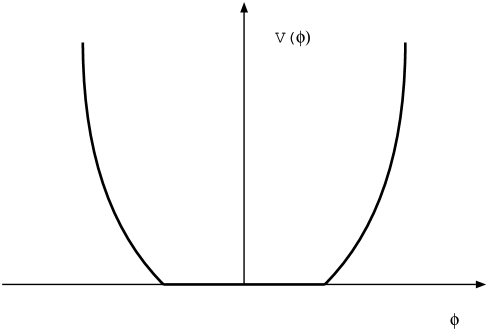
FIG. 1.: Two dimensional projection of the scalar potential in the 3-3-1 model.

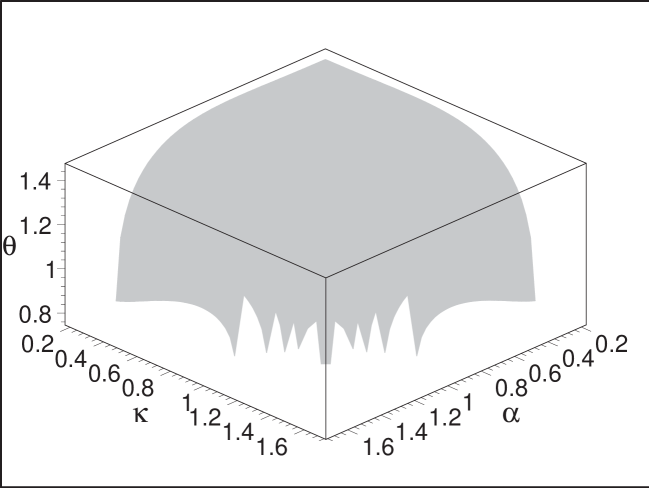
FIG. 2.: Using Eq. (54) we show the surface $V_{331}({\rm min})=0$ with as a function of the exotic quark masses. We have defined $\alpha=m_{J}/v_{\chi}$, $\kappa=m_{j_{1}}/v_{\chi}$ and $\theta=m_{j_{2}}/v_{\chi}$.

REFERENCES

- [1] For a historical review see S. Weinberg, Rev. Mod. Phys. 61, 1 (1989); and Theories of the cosmological constant, unpublished, astro-ph/9610044.
- [2] U. Ellwanger, The Cosmological Constant, Lecture given at the XIV Workshop ‘Beyond the Standard Model”, Bad Honeff 11-14 March 2002, hep-ph/0203252.
- [3] For a clear argumentation see Ya. B. Zel’dovich, Sov. Phys. Usp. 24, 216 (1981); ibid 11, 381 (1968); JETP Lett. 6, 316 (1967); and Pis’ma JETP 6, 883 (1967).
- [4] S. M. Carroll, Living Rev. Rel. 4, 1 (2001); V. Sahni and A. Starobinsky, Int. J. Mod. Phys. D 9, 373 (2000).
- [5] T. Padmanabhan, Cosmological constant – The Weight of the vacuum, hep-th/0212290, to be published in Phys. Rep.
- [6] Some examples are A. D. Dolgov, Phys. Rev. D 55, 5881 (1997); E. Witten, Int. J. Mod. Phys. 10, 1247 (1995); S. Deser and B. Zumino, Phys. Rev. Lett. 38, 1833 (1977); See also Ref. [1].
- [7] S. Weinberg, The cosmological constant problems, astro-ph/0005265, Talk given at 4th International Symposium on Sources and Detection of Dark Matter in the Universe (DM2000), Marina del Rey, CA, February, 2000; H. Martel, P. Shapiro and S. Weinberg, Astrophys. J. 492, 29 (1998).
- [8] N. Bahcall, J. P. Ostriker, S. Perlmutter and P. J. Steinhardt, Science, 284, 1481 (1999).
- [9] E. Witten, The cosmological constant from the viewpoint of string theory, Lecture at 4th International Symposium on Sources and Detection of Dark Matter in the Universe (DM2000), Marina del Rey, CA, February, 2000, hep-ph/0002297.
- [10] J. Dreitkein, Phys. Rev. Lett. 33, 1243 (1974); A. Linde, JETP Lett. 19, 183 (1974); M. Veltman, Phys. Rev. Lett. 34, 777 (1975).
- [11] S. Perlmutter et al., Astrophys. J. 517, 565 (1999); A. G. Riess et al., Astron. J. 116, 1009 (1998).
- [12] E. E. Falco, C. S. Kochanek and J. A. Muñoz, Astrophys. J. 494, 47 (1998).
- [13] P. de Bernardis et al., Nature, 404, 955 (2000).
- [14] For more recent results see: Boomerang experiments, C. B. Netterfield et al., Astrophys. J. 568, 38 (2002); DASI experiment N. W. Halverson et al., Astrophys. J. 571, 604 (2002); MAXIMA experiment A. T. Lee et al., Astrophys. J. Lett. 561, 1 (2001).
- [15] K. Hagiwara et al. (Particle Data Group), Phys. Rev. D 66, 1 (2002).
- [16] G. E. A. Matsas, J. C. Montero, V. Pleitez and D. A. T. Vanzella, Dark matter: the top of the iceberg? in Conference on Topics in Theoretical Physics-II, Festschrift for A. H. Zimerman, edited by H. Aratyn, L. A. Ferreira and J. F. Gomes, (Instituto de Física Teórica, São Paulo 1988, p. 219), hep-ph/9810456; P. B. J. Peebles and A. Vilenkin, Phys. Rev. D 60, 103506 (2000).
- [17] V. Pleitez and M. D. Tonasse, Phys. Rev. D 48, 2353 (1993); T. V. Duong and E. Ma, Phys. Lett. B316, 307 (1993); J. C. Montero, C. A. de S. Pires and V. Pleitez, Phys. Rev. D 65, 093017 (2002).
- [18] F. Pisano and V. Pleitez, Phys. Rev. D 46, 410(1992); R. Foot, O. F. Hernandez, F. Pisano and V. Pleitez, Phys. Rev. D 47, 4158 (1993); P. H. Frampton, Phys. Rev. Lett. 69, 2889 (1992).
- [19] J. F. Gunion, H. E. Haber, G. L. Kane and S. Dawson, The Higgs Hunter’s Guide (Addison-Wesley, Reading, MA, 1990); Santos, S. M. Oliveira and A. Barroso, hep-ph/0112202.
- [20] ALEPH Collaboration, DELPHI Collaboration, L3 Collaboration, OPAL Collaboration, the LEP Higgs Working Group, Search for the Standard Model Higgs Boson at LEP, hep-ph/0107029R.
- [21] M. Sher, Phys. Rep. 179, 273 (1989).
- [22] S. P. Martin, A supersymmetry primer, unpublished, hep-ph/9709356; J. D. Lynkken, Introduction to supersymmetry, unpublished, hep-th/9612114; H. P. Nilles, Phys. Rep. 110, 1 (1984).
- [23] H. E. Haber e G. L. Kane, Phys. Rep. 117, 75 (1985).
- [24] For more details of the scalar potential see M. D. Tonasse, Phys. Lett. B 381, 191 (1996); N. T. Anh, N. A. Ky and H. N. Long, Int. J. Mod. Phys. A16, 541 (2001).
- [25] J. C. Montero, V. Pleitez and O. Ravinez, Phys. Rev. D 60, 076003 (1999).
- [26] U. Schwickerath, (Final) Higgs Results from LEP, hep-ph/0205126. See also M. Carena et al., Tevatron Higgs working group report, hep-ph/0010338.
- [27] P. Jain and S. D. Joglekar, Phys. Lett. B, 407, 151 (1997).
- [28] S. Coleman and E. Weinberg, Phys. Rev. D 7, 1888 (1973).
- [29] R. Jackiw, Phys. Rev D 9, 1686 (1974).
- [30] M. Bando, Progr. Theor. Phys. 90, 405 (1993).
- [31] R. D. Peccei, J. Solá, and C. Wetterich, Phys. Lett. B195, 183 (1987).
- [32] P. Das, P. Jain and W. McKay, Phys. Rev. D59, 055011 (1999).
- [33] A. Vilenkin, talk given at “The dark Universe” (Space Telescope Institute) and PASCOS-2001 in April 2001, hep-th/0106083; V. Sahni, Class. Quant. Grav. 19, 3435 (2002).
- [34] A. Guth, Phys. Rep. 333, 555 (2000) and references therein.
- [35] R. N. Mohapatra and G. Senjanović, Phys. Rev. D 12, 1502 (1979) and references therein.
- [36] V. A. Miransky, Dynamical Symmetry Breaking in Quantum Field Theories (World Scientific, Singapore, 1993).
- [37] W. A. Bardeen, A. J. Buras, D. W. Duke and T. Muta, Phys. Rev. D 18, 3998 (1978).