TPI–MINN–02/07

UMN–TH–2047/02

April 2002

The Forward–Backward Asymmetry of $B\rightarrow(\pi,K)\ell^{+}\ell^{-}$: Supersymmetry at Work

D. A. Demir, Keith A. Olive,

Theoretical Physics Institute, University of Minnesota, Minneapolis, MN 55455

and

M.B. Voloshin

Theoretical Physics Institute, University of Minnesota, Minneapolis, MN 55455

and

Institute of Theoretical and Experimental Physics, Moscow 117218

We analyze the forward–backward asymmetry of the decays $B\rightarrow(\pi,K)\ell^{+}\ell^{-}$ with $\ell=\mu,$ or $\tau$ in the framework of the constrained minimal supersymmetric standard model. We find that, the asymmetry is enhanced at large $\tan\beta$ and depends strongly on the sign of the $\mu$ parameter. For $\mu>0$, the asymmetry is typically large and observable whereas for $\mu<0$, it changes the sign and is suppressed by an order of magnitude. Including cosmological constraints we find that the asymmetry has a maximal value of about 30 %, produced when Higgs- and gauge- induced flavor violations are of comparable size, at a value of $\tan\beta\simeq 35$. The present constraints from the $B$–factories are too weak to constrain parameter space, and the regions excluded by them are already disfavoured by at least one of $\mbox{BR}(B\rightarrow X_{s}\gamma)$, $g-2$, and/or cosmology. The size of the asymmetry is mainly determined by the flavor of the final state lepton rather than the flavor of the pseudoscalar.

1 Introduction

There are sound theoretical and experimental reasons for studying flavor–changing neutral current (FCNC) processes. Such transitions, being forbidden at tree level, provide stringent tests of the standard model (SM) at the loop level. Besides, FCNCs form a natural arena for discovering indirect effects of possible TeV–scale extensions of the SM such as supersymmetry. Among all the FCNC phenomena, the rare decays of the $B$ mesons are particularly important as many of the nonperturbative effects are small and under control.

In addition to having already determined the branching ratio of $B\rightarrow X_{s}\gamma$ [1] and the CP asymmetry of $B\rightarrow J/\psi K$ [2], experimental activity in $B$ physics, has begun to probe FCNC phenomena in semileptonic $B$ decays [3, 4, 5, 6]. Therefore, with increasing data and statistics, these experiments are expected to give precise measurements on long– and short–distance effects in semileptonic decays, $e.g.$ $B\rightarrow P\ell^{+}\ell^{-}$ ($P=K,\pi$) and $B\rightarrow V\ell^{+}\ell^{-}$ ($V=K^{\ast},\rho$). The key physical quantities that can be measured are the branching ratios, CP asymmetries and several lepton asymmetries.

In searching for the physics beyond the SM it is often necessary to deal with quantities that differ significantly from their SM counterparts. This is because there are large uncertainties coming from the hadronic form factors making it hard to disentangle new physics effects from those of the hadronic dynamics. For this reason, the pseudoscalar channel $B\rightarrow P\ell^{+}\ell^{-}$ provides a unique opportunity, since the forward–backward asymmetry $\mbox{A}_{\small\mbox{FB}}$ in this channel is extremely small in the SM (due to a suppression of order $m_{\ell}m_{b}/M_{W}^{2}$), and this remains true in any of its extensions unless a scalar–scalar type four–fermion operator such as

$$\Delta{\cal{A}} = \frac{\alpha G_{F}}{\sqrt{2}\pi}\ V_{tb}V_{tq}^{\ast}\ {\cal{C}}(m_{b})\ \overline{q_{L}}b_{R}\cdot\overline{\ell}\ell$$ (1)

provides a significant contribution to the decay amplitude. Clearly, such operator structures can arise only from the exchange of a scalar between the quark and lepton lines with flavor–violating couplings to the quarks. For instance, by extending the SM Higgs sector to two SU(2) doublets, operator structures of the form (1) can be generated [7] excluding the possibility of $ad$ $hoc$ tree level FCNCs. Although the coefficient ${\cal{C}}(m_{b})$ in eq.(1) is still proportional to the lepton mass, it can receive an enhancement when the ratio of the two Higgs vacuum expectation values, $\tan\beta$ is large.

Supersymmetry (SUSY), is one of the most favoured extensions of the SM which stabilizes the scalar sector against ultraviolet divergences, and naturally avoids the dangerous tree level FCNC couplings by coupling the Higgs doublet $H_{u}$ ($H_{d}$) to up–type quarks (down–type quarks and charged leptons). The soft–breaking of SUSY at the weak scale generates ($i$) a variety of new sources for tree level flavor violation depending on the structure of the soft terms, and ($ii$) radiatively generates various FCNC couplings even if the flavor violation is restricted to the CKM matrix. The first effect, which cannot be determined theoretically, is strongly constrained by the FCNC data [8], and therefore, as a predictive case, it is convenient to restrict all flavor–violating transitions to the charged–current interactions where they proceed via the known CKM angles. This is indeed the case in various SUSY–breaking schemes where hidden sector breaking is transmitted to the observable sector via flavor–blind interactions $e.g.$ gauge–mediated and minimal gravity–mediated scenarios. This minimal flavor violation scheme adopted here is well motivated by minimal supergravity in which all scalars receive a common soft mass, $m_{0}$, at the unification scale.

The common origin for scalar masses is one of the parameter restrictions which define the constrained version of the supersymmetric standard model (CMSSM). The low energy sparticle spectrum in the CMSSM is specified entirely by four parameters, and one sign. In addition to $m_{0}$ and $tan\beta$, the remaining mass parameters are the gaugino masses and supersymmetry breaking trilinear mass terms. These too, are assumed to have common values, $m_{1/2}$ and $A_{0}$, at the unification scale. In principle, there are two additional parameters, the Higgs mixing mass, $\mu$, and the supersymmetry breaking bilinear mass term, $B$, but since it is common to choose $\tan\beta$ as a free parameter and since we fix the sum of the squares of the two Higgs vevs with $M_{Z}$, these two parameters are fixed by the requirements of low energy electroweak symmetry breaking. One is left simply with a sign ambiguity for $\mu$. Therefore, the parameters which define a CMSSM model are $\{m_{1/2},m_{0},A_{0},\tan\beta$ and $sgn(\mu)\}$.

Although flavor violation is restricted to the CKM matrix, radiative effects still generate FCNC transitions among which those that are enhanced at large values of $\tan\beta$ are particularly important as the LEP era ended with a clear preference to large values of $\tan\beta$ [9]. Indeed, it is known that there are large $\tan\beta$–enhanced threshold corrections to the CKM entries [10] allowing for Higgs–mediated FCNC transitions [11]. For instance, the holomorphic mass term for down–type quarks $H_{d}QD^{c}$ acquires a non-holomorphic correction $H_{u}^{\dagger}QD^{c}$ where the latter term proportional to $\tan\beta/16\pi^{2}$, which is not necessarily small at large $\tan\beta$.

In what follows, we will compute the forward–backward asymmetry of $B\rightarrow(\pi,K)\ell^{+}\ell^{-}$ decays in the MSSM. After deriving the scalar exchange amplitudes (1), we discuss several theoretical and experimental issues and then identify the regions of SUSY parameter space for which the asymmetry is enhanced. We compare our results with existing experimental and cosmological constraints.

2 $B\rightarrow(\pi,K)\ell^{+}\ell^{-}$ in Supersymmetry

In general, the semileptonic decays $B\rightarrow(\pi,K)\ell^{+}\ell^{-}$ proceed via the quark transitions $b\rightarrow(s,d)\ell^{+}\ell^{-}$. The decay amplitude has the form

$${\cal{A}} = \frac{\alpha G_{F}}{\pi\sqrt{2}}\ V_{tb}V_{tq}^{\star}\ \Bigg{[}{\cal{C}}_{7}^{eff}(m_{b})\ \overline{q_{L}}i\sigma_{\mu\nu}k^{\nu}b_{R}\overline{\ell}\gamma^{\mu}\ell+{\cal{C}}_{9}^{eff}(m_{b},s)\ \overline{q_{L}}\gamma_{\mu}b_{L}\overline{\ell}\gamma^{\mu}\ell$$ (2)

$$+ {\cal{C}}_{10}(m_{b})\ \overline{q_{L}}\gamma_{\mu}b_{L}\overline{\ell}\gamma^{\mu}\gamma_{5}\ell+{\cal{C}}(m_{b})\ \overline{q_{L}}b_{R}\overline{\ell}\ell+\widehat{{\cal{C}}}(m_{b})\ \overline{q_{L}}b_{R}\overline{\ell}\gamma_{5}\ell\Bigg{]}$$

where $k_{\nu}=-(2m_{b}/q^{2})q_{\nu}$ with $q^{2}\equiv sM_{B}^{2}$ being the dilepton invariant mass. The Wilson coefficients, ${\cal{C}}_{7},{\cal{C}}_{9}$, and ${\cal{C}}_{10}$ have been computed to leading order in [12]. Higher order ${\cal{O}}(\alpha_{s})$ corrections, which are available for small $s$ in the SM [13], will not be considered. The coefficients ${\cal{C}}$ and $\widehat{{\cal{C}}}$ will be discussed below.

The kinematical range for the normalized dilepton invariant mass in terms of the lepton and pseudo scalar masses is $4m_{\ell}^{2}/M_{B}^{2}\leq s\leq(1-M_{P}/M_{B})^{2}$ which includes the vector charmonium resonances $J/\psi,\psi^{\prime},\psi^{\prime\prime},\cdots$ whose effects are included in the ${\cal{C}}_{9}^{eff}(m_{b},s)$. Moreover, the four–fermion operators for the light quarks develop nonvanishing matrix elements, and these are also included in ${\cal{C}}_{9}^{eff}(m_{b},s)$. At higher orders in $\alpha_{s}$, these effects contribute to ${\cal{C}}_{7}^{eff}(m_{b})$ as well [13].

The electromagnetic dipole coefficient ${\cal{C}}_{7}^{eff}(m_{b})$ is contributed by graphs with the W boson, charged Higgs, and chargino penguins. The chargino contribution increases linearly with $\tan\beta$ at leading order [12], and the inclusion of SUSY threshold corrections strengthens this dependence [14]. This coefficient is directly constrained by the $B\rightarrow X_{s}\gamma$ decay rate, and the experimental bounds can be satisfied with a relatively light charged Higgs at very large values of $\tan\beta$. On the other hand, the coefficient of the vector–vector operator ${\cal{C}}_{9}^{eff}(m_{b},s)$ is generated by box diagrams, and carries a long–distance piece coming from the matrix elements of the light quark operators as well as the intermediate charmonium states [15]. Finally, the coefficient of the vector–pseudovector operator ${\cal{C}}_{10}(m_{b})$ is generated by box graphs and is scale independent. Both coefficients ${\cal{C}}_{9}^{eff}(m_{b},s)$ and ${\cal{C}}_{10}(m_{b})$ are less sensitive to $\tan\beta$ than is ${\cal{C}}_{7}^{eff}(m_{b})$.

Within the SM, these coefficients typically have the values ${\cal{C}}_{7}^{eff}(m_{b})\approx-0.3$, ${\cal{C}}_{9}^{eff}(m_{b},s)\approx 4.4$ (excluding its long–distance part), and ${\cal{C}}_{10}(m_{b})\approx-4.7$ [15] which, however, are allowed to vary considerably within the existing bounds [16]. The inclusion of SUSY contributions, for instance, implies large variations in ${\cal{C}}_{7}^{eff}(m_{b})$ (even changing its sign), and typically a $\sim 10\%$ variation in ${\cal{C}}_{9}^{eff}(m_{b},s)$ and ${\cal{C}}_{10}(m_{b})$ [17].

The scalar–scalar operators in the decay amplitude are generically induced by the exchange of the Higgs scalars and suffer invariably from the $m_{\ell}m_{b}/M_{W}^{2}$ suppression. Therefore, these operators are completely negligible in the SM. However, in the MSSM, this suppression is overcome by large $\tan\beta$ effects where the charged Higgs–top diagram is proportional to $\tan^{2}\beta$, and the chargino–stop diagram is $\sim{\cal{O}}(\tan^{3}\beta)$. In more explicit terms, $\widehat{{\cal{C}}}(m_{b})=-{\cal{C}}_{10}(m_{b})$, and

$${\cal{C}}(m_{b}) = \frac{2m_{b}m_{\ell}G_{F}}{\sqrt{2}}\ \frac{1}{4\pi\alpha}\ \frac{1}{(1+\epsilon_{g}\tan\beta)(1+(\epsilon_{g}+h_{t}^{2}\epsilon_{h})\tan\beta)}\$$ (3)

$$\times \left[\tan^{2}\beta f(x_{tH})-\epsilon_{\mu}\tan^{3}\beta x_{tA}\frac{M_{\chi^{\pm}}A_{t}}{M_{\tilde{t}_{1}}^{2}-M_{\chi^{\pm}}^{2}}\ \left(f(x_{\chi^{\pm}\tilde{t}_{2}})-f(x_{\tilde{t}_{1}\tilde{t}_{2}})\right)\right]$$

where $\epsilon_{\mu}$ is the sign of the $\mu$ parameter, $\chi^{\pm}$ is the lighter chargino, $x_{ij}=m_{i}^{2}/m_{j}^{2}$, $f(x)=x\log{x}/(1-x)$, and the parameters $\epsilon_{g}$ and $\epsilon_{h}$, which are typically ${\cal{O}}(10^{-2})$, are defined in [11, 14]. Finally, $h_{t}$ is the top quark Yukawa coupling, $M_{\tilde{t}_{1}}$ is the light stop mass, and $A_{t}$ is the low energy value of the SUSY breaking top-Yukawa trilinear mass term obtained from $A_{0}$ by the running of the RGEs. Clearly, the charged Higgs contribution, which is the dominant one in two–doublet models [7], is subleading compared to the chargino contribution. The sign of ${\cal{C}}(m_{b})$ depends explicitly on $\epsilon_{\mu}$. Therefore, the forward–backward asymmetry in $B\rightarrow(\pi,K)\ell^{+}\ell^{-}$ decays depends strongly on the sign of the $\mu$ parameter.

From the experimental point of view, it is useful to analyze the normalized forward–backward asymmetry defined as

$$\mbox{A}_{\mbox{\small FB}}(P\ell^{+}\ell^{-})=\frac{\int_{-1}^{0}dz\frac{d^{2}\Gamma}{dzds}-\int_{0}^{1}dz\frac{d^{2}\Gamma}{dzds}}{\int_{-1}^{0}dz\frac{d^{2}\Gamma}{dzds}+\int_{0}^{1}dz\frac{d^{2}\Gamma}{dzds}}$$ (4)

where $z=\cos\theta$, $\theta$ being the angle between the momenta of $P$ and $\ell^{+}$. A direct calculation gives the explicit expression

$$\mbox{A}_{\mbox{\small FB}}(P\ell^{+}\ell^{-})=-\frac{\lambda^{1/2}(s)v(s)t_{\ell}\mbox{Re}[A_{79}(s)]A(s)}{\Sigma(s)}$$ (5)

where

$$\Sigma(s) = \lambda(s)(1-v(s)^{2}/3)\left[|A_{79}(s)|^{2}+A_{10}(s)^{2}\right]+t_{\ell}t_{P}A_{10}(s)^{2}$$ (6)

$$+ st_{\ell}\left[(B_{10}(s)-A(s))^{2}+v(s)^{2}A(s)^{2}\right]$$

$$+ 2t_{\ell}(1-t_{P}/4-s)[B_{10}(s)-A(s)]A_{10}(s)\;.$$

Here $t_{\ell}=4m_{\ell}^{2}/M_{B}^{2}$, $t_{P}=4M_{P}^{2}/M_{B}^{2}$, $\lambda(s)=(1-s-t_{P}/4)^{2}-st_{P}$, $v(s)=(1-t_{\ell}/s)^{1/2}$ and

$$A_{79}(s) = {\cal{C}}_{9}^{eff}(m_{b},s)f_{+}(s)-{\cal{C}}_{7}^{eff}(m_{b})f_{7}(s)\,,$$

$$A_{10}(s) = {\cal{C}}_{10}(m_{b})f_{+}(s)\;\>\>,\>\>\>B_{10}(s)={\cal{C}}_{10}(m_{b})(f_{+}(s)+f_{-}(s))$$

$$A(s) = {\cal{C}}(m_{b})\ \frac{M_{B}^{2}}{2m_{b}m_{\ell}}\ [(1-M_{P}^{2}/M_{B}^{2})f_{+}(s)+sf_{-}(s)]$$ (7)

where $f_{7}(s)=(2m_{b})/(M_{B}+M_{P})f_{T}(s)$. The form factors $f_{+}$, $f_{-}$ and $f_{T}$ are not measured at present and one has to rely on theoretical predictions. In what follows we use the results of the calculation [18] of these form factors from QCD sum rules for both $B\rightarrow K$ and $B\rightarrow\pi$ transitions.

In general, the hadronic form factors are uncertain by $\sim 15\%$, and this translates into an uncertainty of approximately $35\%$ in the branching ratio. Especially for low $s$, below the charmonium resonances, the theoretical prediction for the branching ratio contains large uncertainties [19]. Therefore, theoretically the large dilepton mass region is more tractable. On top of the form factor uncertainties, there are further problems in treating the contributions of the charmonium resonances (embedded in the Wilson coefficient ${\cal{C}}_{9}^{eff}(m_{b},s)$). For instance, the recent BELLE experiments [3], subtract such resonance contributions by vetoing the range $0.322\mathrel{\hbox to0.0pt{\lower 3.0pt\hbox{\hskip 0.0pt$\sim$}\hss}\raise 1.0pt\hbox{$<$}}s\mathrel{\hbox to0.0pt{\lower 3.0pt\hbox{\hskip 0.0pt$\sim$}\hss}\raise 1.0pt\hbox{$<$}}0.362$. Then the experimental bound on the branching ratio turns out to be

$$0.0328\leq 10^{6}\times\mbox{BR}(B\rightarrow K\mu^{+}\mu^{-})\leq 2.395\>\>\>\mbox{at}\>\>90\%\>\mbox{C.L.}$$ (8)

which we will take into account in making the numerical estimates below. It can be also noted that the same decay mode has not been observed by BABAR: $\mbox{BR}(B\rightarrow K\mu^{+}\mu^{-})<4.5\times 10^{-6}\>\>\mbox{at}\>\>90\%\>\mbox{C.L.}$ [4]. In addition, the vector kaon final states have not been observed yet: $\mbox{BR}(B\rightarrow K^{\star}\mu^{+}\mu^{-})<3.6\times 10^{-6}\>\>\mbox{at}\>\>90\%\>\mbox{C.L.}$ [3, 4]. One notes that, the asymmetry is large in regions of the parameter space where the branching ratio is depleted, and therefore, the BELLE lower bound on $B\rightarrow K\mu^{+}\mu^{-}$ is an important constraint which can prohibit the asymmetry taking large marginal values. Clearly, in the presence of ${\cal{C}}(m_{b})$, which can take large values in SUSY, the would–be experimental constraints on the $C_{10}(m_{b})$–${\cal{C}}_{9}^{eff}(m_{b},s)$ plane are lifted.

Furthermore, the pure leptonic decay modes, $B_{s,d}\rightarrow\ell^{+}\ell^{-}$, depend directly on the Wilson coefficients $C_{10}(m_{b})$, ${\cal{C}}(m_{b})$ and $\widehat{{\cal{C}}}(m_{b})$. In the SM, $\mbox{BR}(B_{s}\rightarrow\mu^{+}\mu^{-})\approx 10^{-9}$ which is approximately three orders of magnitude below the present bounds $\mbox{BR}(B_{s}\rightarrow\mu^{+}\mu^{-})<2.6\times 10^{-6}$ [20]. The SUSY contributions, especially at large $\tan\beta$, can enhance the SM prediction typically by an order of magnitude, and the bounds can even be violated in certain corners of the parameter space [21]. In what follows the constraints from $B_{s}\rightarrow\mu^{+}\mu^{-}$ as well as the muon $g-2$ (as they are directly correlated [22]) will be taken into account. We will refer to the constraints from $B\rightarrow(K,K^{\star})\mu^{+}\mu^{-}$ and $B_{s,d}\rightarrow\ell^{+}\ell^{-}$ collectively as $B$–factory constraints.

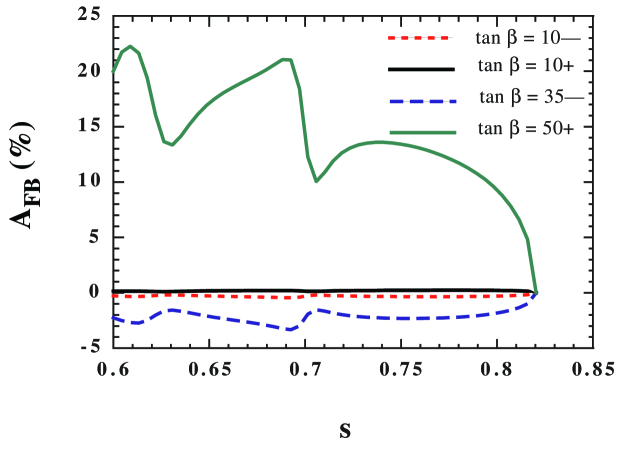
Figure 1: The dependence of $\mbox{A}_{\mbox{\small FB}}(K\tau^{+}\tau^{-})$ on the normalized dilepton invariant mass, $s=q^{2}/M_{B}^{2}$, for various (allowed) points in the SUSY parameter space. Each curve is labeled as $\tan\beta\ \epsilon_{\mu}$ where $(m_{1/2},m_{0})=(400,100),(400,100),(900,700),(1200,600)\ {\rm GeV}$ from top to bottom. One notices that the asymmetry is typically small for $\mu<0$ as was noted at various instances before.

For the constraints on the SUSY parameter space to make sense it is necessary to be far from the regions of large hadronic uncertainties, and thus, below we will restrict the range of $s$ to lie well above the charmonium resonances and well below the kinematical end point. In Fig. 1, we show the variation of the asymmetry with the normalized dilepton invariant mass, $s=q^{2}/M_{B}^{2}$ for various values of the SUSY parameters (see below for further discussion of these choices). The irregularities in the $s$–dependence of the asymmetry are similar to those in the $B\rightarrow K^{\star}\ell^{+}\ell^{-}$ decay. The various bumps and valleys come from the relative sizes of individual terms contributing to $\mbox{A}_{\mbox{\small FB}}$. It should be noted that in the region around the value $s=0.75$, the $s$ dependence of the asymmetry is rather smooth. Therefore, in forming the constant asymmetry contours in the space of SUSY parameters we will take $s=0.75$ (corresponding to $q^{2}=20.1\ {\rm GeV}^{2}$).

At low values of the asymmetry one should also take into account the final state electromagnetic interactions. Indeed, photon exchange between the lepton and $P=K,\pi$ lines is expected to induce an asymmetry ${\cal{O}}(\alpha/\pi)$ implying that only asymmetries $\mbox{A}_{\mbox{\small FB}}$ larger than $\sim 1\%$ can be trusted to follow from SUSY effects, unless the interplay with the electromagnetic corrections is explicitly taken into account. For large values of asymmetry, when the observation of the effect becomes feasible, higher order QCD effects (not yet calculated) can in principle modify our results somewhat. However, it is highly unlikely that these corrections will dramatically reduce the asymmetry discussed here.

One should also note that in the limit of exact $SU(3)$ flavor symmetry, the asymmetries in $B\rightarrow K\ell^{+}\ell^{-}$ and $B\rightarrow\pi\ell^{+}\ell^{-}$ decays must be the same. Due to $SU(3)$ breaking effects, which show up in different parameterizations of the form factors $f_{+}$, $f_{-}$ and $f_{7}$ for $B\rightarrow\pi$ and $B\rightarrow K$ transitions [18], their asymmetries are expected to differ slightly. Clearly it is the lepton flavor that largely determines the size of the asymmetry, rather than the flavor of the final state pseudoscalar.

Finally, before starting to scan the SUSY parameter space, it is worth while discussing the sensitivity of $\mbox{A}_{\mbox{\small FB}}$ to some of the parameters. First of all, as $\tan\beta$ grows, two of the Wilson coefficients, ${\cal{C}}_{7}^{eff}(m_{b})$ and ${\cal{C}}(m_{b})$, grow rapidly up to the bounds obtained from rates of the decays $(B\rightarrow X_{s}\gamma)$ and $(B\rightarrow K\mu^{+}\mu^{-})$. Since $\mbox{Re}[{\cal{C}}_{9}^{eff}(m_{b},s)]>0$ and ${\cal{C}}_{7}^{eff}(m_{b})>0$, $\mbox{Re}[A_{79}(s)]$ increases with $\tan\beta$. However, this increase is much milder than the $\tan^{3}\beta$ dependence of ${\cal{C}}(m_{b})$ causing $A(s)$ to take large negative (positive) values for $\mu>0$ ($\mu<0$). Therefore, large $\tan\beta$ effects influence not only the numerator of Eq. (5) but also the denominator $\Sigma(s)$ (proportional to the differential branching fraction) via the destructive (constructive) interference with $B_{10}(s)$ ($C_{10}(m_{b})$ remains negative in SUSY) for $\mu>0$ ($\mu<0$). However, as $\tan\beta$ keeps growing, depending on the rest of the SUSY parameters, the effect of ${\cal{C}}(m_{b})$ eventually becomes more important, and the asymmetry falls rapidly due to the enhanced branching ratio. In this sense, the regions of enhanced asymmetry depend crucially on the sign of the $\mu$ parameter and the specific value of $\tan\beta$. Moreover, as the expression of ${\cal{C}}(m_{b})$ makes clear, there can be sign changes in the asymmetry in certain regions of the parameter space due to the relative sizes of the masses of the lighter chargino and stops. Such effects will also give small asymmetries just like the $\mu<0$ case.

Our work extends a previous analysis of this asymmetry [23] by including the large gluino exchange effects (contained in the quantity $\epsilon_{g}$ in Eq. (3)) and the explicit dependence on the sign of the $\mu$ parameter. In addition, we go beyond the work in [23] as well as in the preceding work [24] by resumming the higher order $\tan\beta$ terms which increases the validity of the analysis at large values of $\tan\beta$ [14]. We note that a computation of the large $\tan\beta$ effects can be carried out in the gaugeless limit [11] which eliminates some of the diagrams considered in [23].

In the numerical analysis below, we will analyze the forward–backward asymmetry of the decays $B\rightarrow P\ell^{+}\ell^{-}$ by taking into account the above–mentioned constraints from $B$ factories as well as other collider and cosmological constraints. We will be searching for those regions of the SUSY parameter space in which the asymmetry is enhanced. In particular, we will be particularly interested in the sensitivity of the asymmetry to $\tan\beta$, the sign of the $\mu$ parameter, as well as the common scalar mass $m_{0}$ and the gaugino mass $m_{1/2}$.

3 Results

In our analysis, we include several accelerator as well as cosmological constraints. From the chargino searches at LEP [25], we apply the kinematical limit $m_{\chi^{\pm}}\mathrel{\hbox to0.0pt{\lower 4.0pt\hbox{\hskip 1.0pt$\sim$}\hss}\raise 1.0pt\hbox{$>$}}$ 104 GeV. A more careful consideration of the constraint would lead to an unobservable difference in the figures shown below. This constraint can be translated into a lower bound on the gaugino mass parameter, $m_{1/2}$ and is nearly independent of other SUSY parameters. The LEP chargino limit is generally overshadowed (in the CMSSM) by the important constraint provided by the LEP lower limit on the Higgs mass: $m_{h}>$ 114.1 GeV [9]. This holds in the Standard Model, for the lightest Higgs boson $h$ in the general MSSM for $\tan\beta\mathrel{\hbox to0.0pt{\lower 3.0pt\hbox{\hskip 0.0pt$\sim$}\hss}\raise 1.0pt\hbox{$<$}}8$, and almost always in the CMSSM for all $\tan\beta$. The Higgs limit also imposes important constraints on the CMSSM parameters, principally $m_{1/2}$, though in this case, there is a strong dependence on $\tan\beta$. The Higgs masses are calculated here using FeynHiggs [26], which is estimated to have a residual uncertainty of a couple of GeV in $m_{h}$.

We also include the constraint imposed by measurements of $b\rightarrow s\gamma$ [1, 14]. These agree with the Standard Model, and therefore provide bounds on MSSM particles, such as the chargino and charged Higgs masses, in particular. Typically, the $b\rightarrow s\gamma$ constraint is more important for $\mu<0$, but it is also relevant for $\mu>0$, particularly when $\tan\beta$ is large.

The final experimental constraint we consider is that due to the measurement of the anomalous magnetic moment of the muon. The BNL E821 [27] experiment reported a new measurement of $a_{\mu}\equiv{1\over 2}(g_{\mu}-2)$ which deviates by 1.6 standard deviations from the best Standard Model prediction (once the pseudoscalar-meson pole part of the light-by-light scattering contribution [28] is corrected). Although negative values of $\mu$ are no longer entirely excluded [29], the 2-$\sigma$ limit still excludes much of the $\mu<0$ parameter space [30]. $\mu<0$ is allowed so long as either (or both) $m_{1/2}$ and $m_{0}$ are large.

We also apply the cosmological limit on the relic density of the lightest supersymmetric particle (LSP), $\rho_{\chi}=\Omega_{\chi}\rho_{critical}$, and require that

$$0.1<\Omega_{\chi}h^{2}<0.3$$ (9)

The upper limit is rigorous, and assumes only that the age of the Universe exceeds 12 Gyr. It is also consistent with the total matter density $\Omega_{m}\mathrel{\hbox to0.0pt{\lower 3.0pt\hbox{\hskip 0.0pt$\sim$}\hss}\raise 1.0pt\hbox{$<$}}0.4$, and the Hubble expansion rate $h\sim 0.7$ to within about 10 % (in units of 100 km/s/Mpc). On the other hand, the lower limit in (9) is optional, since there could be other important contributions to the overall matter density.

The cosmologically allowed regions in the CMSSM have been well studied [31, 32]. There are generally large, ‘bulk’ regions of parameter space at low to moderate values of $m_{1/2}$ and $m_{0}$ at all values of $\tan\beta$. There are additional regions which span out to large values of $m_{1/2}$ due to co-annihilations with light sleptons, particularly the lighter $\tilde{\tau}$ [33]. At large $\tan\beta$, there are also regions in which the lightest neutralino sits on the s-channel pole of the pseudo-scalar and heavy scalar Higgs producing ‘funnel’-like regions [34, 31]. Finally, there are the so-called ‘focus-point’ regions [35] which are present at very large values of $m_{0}$. Generally, these regions have a lower asymmetry (because of the large value of $m_{0}$), however, at values of $\tan\beta\sim 50$, asymmetries as large as 10% are possible.

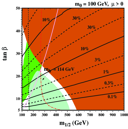
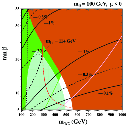
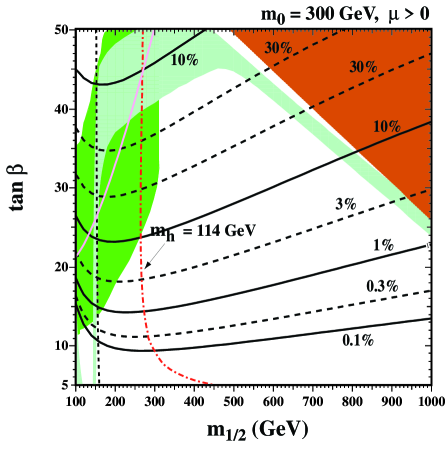
Figure 2: The constant $\mbox{A}_{\mbox{\small FB}}(K\tau^{+}\tau^{-})$ contours in $m_{1/2}$–$\tan\beta$ plane for $A_{0}=0$, with $m_{0}=100$ GeV, $\mu>0$ (a); $m_{0}=100$ GeV, $\mu<0$ (b); $m_{0}=200$ GeV, $\mu>0$ (c); and $m_{0}=300$ GeV, $\mu>0$ (d). We take $m_{t}=175\ {\rm GeV}$ and $m_{b}(m_{b})_{SM}^{\overline{MS}}=4.25\ {\rm GeV}$. In all of the panels the black dashed line shows the 104 GeV chargino mass contour, the dot–dashed (red) curve stands for $m_{h}=114\ {\rm GeV}$ (evaluated using the FeynHiggs code [26]). The light (turquoise) areas are the cosmologically preferred regions with $0.1\leq\Omega_{\chi}h^{2}\leq 0.3$. In the dark (brick–red) shaded areas the LSP is $\widetilde{\tau}_{1}$ and thus excluded. The medium (green) shaded regions are excluded by $\mbox{BR}(B\rightarrow X_{s}\gamma)$. The light (violet) curve shows the $g_{\mu}-2$ (the area to the right of which is allowed).

In Fig. 2a, we show the contours of constant $\mbox{A}_{\mbox{\small FB}}(K\tau^{+}\tau^{-})$ in $m_{1/2}$–$\tan\beta$ plane for $A_{0}=0$, $m_{0}=100\ {\rm GeV}$ and $\mu>0$. The constraints discussed above are shown by various curves and shaded regions. The nearly vertical dashed (black) line at the left of the figure shows the chargino mass constraint. Allowed regions are to the right of this line. The dot-dashed Higgs mass contour (red) labeled 114 GeV, always provides a stronger constraint. Allowed regions are again to the right of this curve. However, one should be aware that there is a theoretical uncertainty in the Higgs mass calculation, making this limit somewhat fuzzy. The light (violet) solid curve shows the position of the 2-$\sigma$ $g-2$ constraint, which again excludes small values of $m_{1/2}$. In the dark (red) shaded region covering much of the upper left half of the plane, the lighter $\tilde{\tau}$ is either the LSP or is tachyonic. Since there are very strong constraints forbidding charged dark matter, this region is excluded. The medium shaded (green) region shows the exclusion area provided by the $b\to s\gamma$ measurements. Finally the light (turquoise) shaded region shows the area preferred by cosmology. Outside this shaded region, the relic density is too small and is technically not excluded.

Putting all of the constraints together, we find that for this value of $m_{0}=100$  GeV and $\mu>0$, the allowed region is bounded by $300\ {\rm GeV}\mathrel{\hbox to0.0pt{\lower 3.0pt\hbox{\hskip 0.0pt$\sim$}\hss}\raise 1.0pt\hbox{$<$}}m_{1/2}\mathrel{\hbox to0.0pt{\lower 3.0pt\hbox{\hskip 0.0pt$\sim$}\hss}\raise 1.0pt\hbox{$<$}}500\ {\rm GeV}$ and $5\mathrel{\hbox to0.0pt{\lower 3.0pt\hbox{\hskip 0.0pt$\sim$}\hss}\raise 1.0pt\hbox{$<$}}\tan\beta\mathrel{\hbox to0.0pt{\lower 3.0pt\hbox{\hskip 0.0pt$\sim$}\hss}\raise 1.0pt\hbox{$<$}}20$. In the allowed region, the forward-backward asymmetry varies rapidly from very small (unobservable) values up to $10\%$. There is a wide region with an observable $1$–$10\%$ asymmetry though the $10\%$ region is quite narrow (restricted to $\tan\beta\sim 20$).

In Fig. 2b, we show the corresponding result for the opposite sign of $\mu$. While the cosmologically allowed region is qualitatively similar to the $\mu>0$ case and the Higgs limit is slightly stronger, we see that the $b\to s\gamma$ constraint is significantly stronger. Indeed, the combined constraints from $b\to s\gamma$ and a $\tilde{\tau}$ LSP exclude $\tan\beta\mathrel{\hbox to0.0pt{\lower 4.0pt\hbox{\hskip 1.0pt$\sim$}\hss}\raise 1.0pt\hbox{$>$}}15$ for this value of $m_{0}$ and $\mu<0$. The 2-$\sigma$ constraint from $g-2$ is also significantly stronger and when combined with the $\tilde{\tau}$ LSP constraint now exclude values of $\tan\beta\mathrel{\hbox to0.0pt{\lower 4.0pt\hbox{\hskip 1.0pt$\sim$}\hss}\raise 1.0pt\hbox{$>$}}8$.

As mentioned earlier, for $\mu<0$ both the sign and size of the asymmetry have changed. In general, the size of the asymmetry is suppressed by an order of magnitude. Clearly, the $b\to s\gamma$ constraint now allows only a small region with a $-0.3$ – $-1\%$ asymmetry. However, when all constraints are combined they exclude almost completely the otherwise allowed regions. At higher values of $m_{0}$, slightly larger asymmetries are possible. At $m_{0}=200$ GeV (with $\mu<0$), $b\to s\gamma$ allows asymmetries as large as $-2$%, however, the $g-2$ data still restricts the asymmetry to values below about $-0.4$ %. Even at large $\tan\beta$ and very large $m_{0}$, we will see below that for $\mu<0$, asymmetries never excced $\sim-1$ %. We note that independent of the sign of $\mu$, the asymmetry is maximized for intermediate values of $\tan\beta$, $i.e.$ it does not monotonically increase with increasing $\tan\beta$ as was already argued earlier. The main conclusion from this figure is that the sign of the $\mu$ parameter must be positive in order to have large observable $\mbox{A}_{\mbox{\small FB}}(K\tau^{+}\tau^{-})$.

We note that there are already $B$–factory constraints due to recent BELLE and BABAR experiments [2, 3, 4]. For $\mu>0$, they exclude a small region (not plotted) with $m_{1/2}\mathrel{\hbox to0.0pt{\lower 3.0pt\hbox{\hskip 0.0pt$\sim$}\hss}\raise 1.0pt\hbox{$<$}}120\ {\rm GeV}$ and $\tan\beta\mathrel{\hbox to0.0pt{\lower 4.0pt\hbox{\hskip 1.0pt$\sim$}\hss}\raise 1.0pt\hbox{$>$}}43.5$ (lying in the region with a charged LSP), whereas for $\mu<0$ the excluded region is shifted to $m_{1/2}\mathrel{\hbox to0.0pt{\lower 3.0pt\hbox{\hskip 0.0pt$\sim$}\hss}\raise 1.0pt\hbox{$<$}}260\ {\rm GeV}$ and $\tan\beta\mathrel{\hbox to0.0pt{\lower 4.0pt\hbox{\hskip 1.0pt$\sim$}\hss}\raise 1.0pt\hbox{$>$}}30.5$ (now lying in the region also excluded by $\mbox{BR}(B\rightarrow X_{s}\gamma)$).

The behaviour observed in Fig. 2a) and b) is subject to large variations once the GUT–scale input parameters are varied. This is seen in Fig. 2c) and d) where the constant asymmetry curves are plotted in $m_{1/2}$–$\tan\beta$ for $\mu>0$, $A_{0}=0$, and $m_{0}=200\ {\rm GeV}$ and $m_{0}=300\ {\rm GeV}$ respectively. It is clear that with increasing $m_{0}$ the cosmologically preferred ‘bulk’ region is shifted towards larger $\tan\beta$ values making it possible to get larger asymmetries. In addition, we see very clearly the effect of $\chi-{\tilde{\tau}}$ coannihilations [33] which extend the cosmological region to high values of $m_{1/2}$. The region below the ‘bulk’ and coannihilation region is excluded as it corresponds to an area with $\Omega h^{2}>0.3$. While the chargino, Higgs, and $g-2$ constraints are only slightly altered at the higher value of $m_{0}$, we see that the charged LSP constraint is relaxed in Fig. 2c) and greatly relaxed in panel d).

For the higher values of $m_{0}$ we see from Fig. 2c) that for $300\ {\rm GeV}\mathrel{\hbox to0.0pt{\lower 3.0pt\hbox{\hskip 0.0pt$\sim$}\hss}\raise 1.0pt\hbox{$<$}}m_{1/2}\mathrel{\hbox to0.0pt{\lower 3.0pt\hbox{\hskip 0.0pt$\sim$}\hss}\raise 1.0pt\hbox{$<$}}800\ {\rm GeV}$ and $25\mathrel{\hbox to0.0pt{\lower 3.0pt\hbox{\hskip 0.0pt$\sim$}\hss}\raise 1.0pt\hbox{$<$}}\tan\beta\mathrel{\hbox to0.0pt{\lower 3.0pt\hbox{\hskip 0.0pt$\sim$}\hss}\raise 1.0pt\hbox{$<$}}40$ the forward-backward asymmetry ranges from $1\%$ to $30\%$ in regions which are not excluded by any experimental or cosmological constraints. In particular, when $350\ {\rm GeV}\mathrel{\hbox to0.0pt{\lower 3.0pt\hbox{\hskip 0.0pt$\sim$}\hss}\raise 1.0pt\hbox{$<$}}m_{1/2}\mathrel{\hbox to0.0pt{\lower 3.0pt\hbox{\hskip 0.0pt$\sim$}\hss}\raise 1.0pt\hbox{$<$}}400\ {\rm GeV}$ and $30\mathrel{\hbox to0.0pt{\lower 3.0pt\hbox{\hskip 0.0pt$\sim$}\hss}\raise 1.0pt\hbox{$<$}}\tan\beta\mathrel{\hbox to0.0pt{\lower 3.0pt\hbox{\hskip 0.0pt$\sim$}\hss}\raise 1.0pt\hbox{$<$}}35$ the asymmetry is well observable with a typical $\sim 30\%$ peak value. Here the $B$–factory constraints are effective for $m_{1/2}\sim 100\ {\rm GeV}$ and $\tan\beta\mathrel{\hbox to0.0pt{\lower 4.0pt\hbox{\hskip 1.0pt$\sim$}\hss}\raise 1.0pt\hbox{$>$}}47.5$, i.e. only a small region in the upper left corner.

For the $m_{0}=300\ {\rm GeV}$ case shown in Fig. 2d), the cosmologically allowed region is now shifted up past the maximum of $\mbox{A}_{\mbox{\small FB}}(K\tau\tau)$, and is now typically $10\%$. Overall the forward-backward asymmetry is larger than 1% in the cosmologically allowed region and extends over the range $300\ {\rm GeV}\mathrel{\hbox to0.0pt{\lower 3.0pt\hbox{\hskip 0.0pt$\sim$}\hss}\raise 1.0pt\hbox{$<$}}m_{1/2}\mathrel{\hbox to0.0pt{\lower 3.0pt\hbox{\hskip 0.0pt$\sim$}\hss}\raise 1.0pt\hbox{$<$}}1000\ {\rm GeV}$ and $25\mathrel{\hbox to0.0pt{\lower 3.0pt\hbox{\hskip 0.0pt$\sim$}\hss}\raise 1.0pt\hbox{$<$}}\tan\beta\mathrel{\hbox to0.0pt{\lower 3.0pt\hbox{\hskip 0.0pt$\sim$}\hss}\raise 1.0pt\hbox{$<$}}50$.

We have also checked some cases with nonzero values of $A_{0}$, assuming it to be either constant ($e.g.$ set to $2\ {\rm TeV}$), or varying in proportion with $m_{1/2}$ ($e.g.$, $A_{0}=2m_{1/2}$). For a variable $A_{0}$, results were not qualitatively different from the results shown here. For a large and fixed value of $A_{0}$, the comsological regions of interest could be very different [36], however, the asymmetry was found to be quantitatively similar as the results shown here. However, we can not claim to have made a systematic examination of the $A_{0}\neq 0$ parameter space.

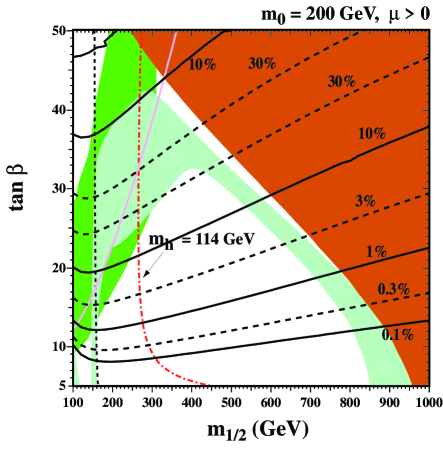
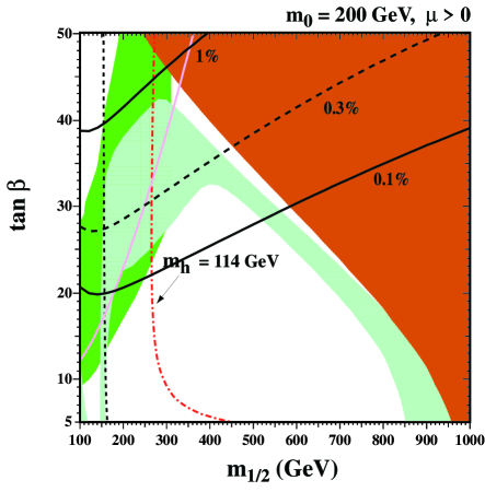
Figure 3: The contours of $\mbox{A}_{\mbox{\small FB}}(\pi\tau^{+}\tau^{-})$ (left panel) and $\mbox{A}_{\mbox{\small FB}}(K\mu^{+}\mu^{-})$ (right panel) for $A_{0}=0$, $m_{0}=200\ {\rm GeV}$ and $\mu>0$. All other curves and shaded regions are taken from Fig. 2c).

In Fig. 3, we show the contours of $\mbox{A}_{\mbox{\small FB}}(\pi\tau^{+}\tau^{-})$ (left panel) and $\mbox{A}_{\mbox{\small FB}}(K\mu^{+}\mu^{-})$ (right panel) for $A_{0}=0$, $m_{0}=200\ {\rm GeV}$ and $\mu>0$. A comparison of the left panel with panel c) of Fig. 2 shows that there is very little difference between $\pi\ell^{+}\ell^{-}$ and $K\ell^{+}\ell^{-}$ final states as far as the asymmetry is concerned. Indeed, as mentioned before, the difference between the asymmetries is a measure of the SU(3) flavor breaking or the different parameterizations of the associated form factors. Therefore, the similarity or dissimilarity of these two figures depends on how the hadronic effects are treated for the kaon and pion final states. On the other hand, the comparison between panel c) of Fig. 2 and the right panel of Fig. 3 shows that the asymmetry is suppressed for the $\mu^{+}\mu^{-}$ final states. The asymmetry does not reach the $1\%$ level in any corner of the allowed regions.

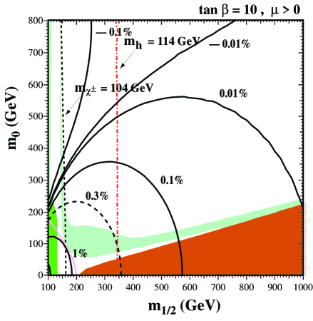
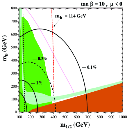
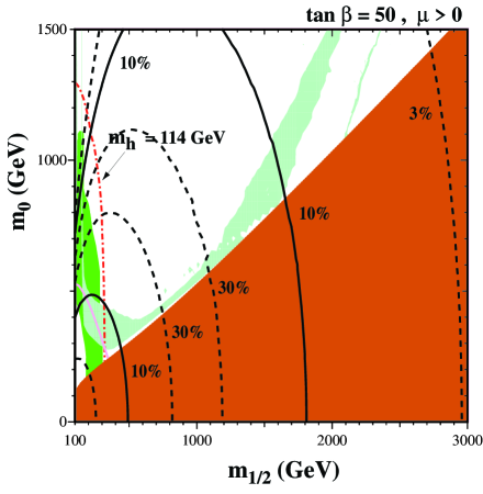
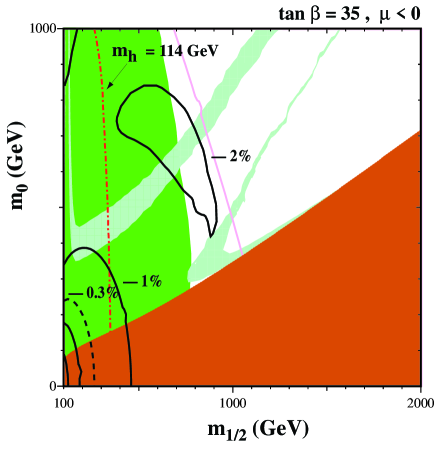
Figure 4: The constant $\mbox{A}_{\mbox{\small FB}}(K\tau^{+}\tau^{-})$ contours in $m_{1/2}$–$m_{0}$ for $A_{0}=0$, and $\tan\beta=10$, $\mu>0$ (a); $\tan\beta=10$, $\mu<0$ (b); $\tan\beta=50$, $\mu>0$ (c); and $\tan\beta=35$, $\mu<0$ (d). Contours and shaded regions are as in Fig. 2

In Fig. 4a), we show the $\mbox{A}_{\mbox{\small FB}}(K\tau^{+}\tau^{-})$ contours as projected onto the $m_{1/2}$–$m_{0}$ plane for $A_{0}=0$, $\tan\beta=10$, $\mu>0$. The curves and shading in this figure are as in Fig. 2. Seen clearly are the ‘bulk’ and coannihilation cosmological regions. The latter traces the border of the $\tilde{\tau}$ LSP region which is now found at the lower right of the figure. The constraints from $b\to s\gamma$ and $g-2$ only exclude a small portion of the parameter plane at the lower left. In this figure, it is the area above the cosmological shaded region which is excluded due to an excessive relic density.

This figure illustrates the dependence of the asymmetries on the chargino and stop masses, and indeed, the asymmetry changes sign at fairly large $m_{0}$ and small $m_{1/2}$. This effect results in a sign change in ${\cal{C}}(m_{b})$ due to the competition between the stop and chargino masses. As Fig. 4a) makes clear, the asymmetry is positive and remains below the $0.3\%$ level yielding essentially no observable signal at all.

An example with $\tan\beta=10$ and $\mu<0$ is shown in Fig. 4b). While the cosmological region is similar to that in panel a), the constraint from $b\to s\gamma$ is significantly stronger, as is the constraint from $g-2$. The latter imply that the asymmetry is never much larger than $-0.1\%$. As one can see, it is difficult to get any observable effect at low values of $\tan\beta$,for any sign of the $\mu$ parameter.

In the lower two panels of Fig. 4, we show the contours of $\mbox{A}_{\mbox{\small FB}}(K\tau^{+}\tau^{-})$ for larger values of $\tan\beta$. As one can see, the ‘bulk’ cosmological regions are pushed to higher values of $m_{0}$ and we also see the appearance of the ‘funnel’ regions where the LSP relic density is primarily controlled by $H,A$ s-channel annihilations. In panel c), there are large positive asymmetries ($\mathrel{\hbox to0.0pt{\lower 4.0pt\hbox{\hskip 1.0pt$\sim$}\hss}\raise 1.0pt\hbox{$>$}}10\%$) in a broad region extending from $(m_{1/2},m_{0})=(300,300)\ {\rm GeV}$ all the way up to $(m_{1/2},m_{0})=(1.8,1.1)\ {\rm TeV}$. The $B$–factory constraints only exclude a small region in the bottom left corner bounded by $m_{0}\mathrel{\hbox to0.0pt{\lower 3.0pt\hbox{\hskip 0.0pt$\sim$}\hss}\raise 1.0pt\hbox{$<$}}200\ {\rm GeV}$ and $m_{1/2}\mathrel{\hbox to0.0pt{\lower 3.0pt\hbox{\hskip 0.0pt$\sim$}\hss}\raise 1.0pt\hbox{$<$}}120\ {\rm GeV}$. Panel d) of Fig. 4, on the other hand, shows that, for negative $\mu$ and large $\tan\beta$, the allowed range of asymmetry is around $-1\%$ never reaching the $-2\%$ level mainly due to the $g_{\mu}-2$ constraint. There are three cosmologically preferred strips, the wider one located in the region $(m_{1/2},m_{0})\mathrel{\hbox to0.0pt{\lower 4.0pt\hbox{\hskip 1.0pt$\sim$}\hss}\raise 1.0pt\hbox{$>$}}(900,700)\ {\rm GeV}$ where the asymmetry is at most $-1\%$. For $\mu<0$ the $B$–factory constraints exclude two small regions bounded by $m_{0}\mathrel{\hbox to0.0pt{\lower 3.0pt\hbox{\hskip 0.0pt$\sim$}\hss}\raise 1.0pt\hbox{$<$}}200\ {\rm GeV}$ and $m_{1/2}\mathrel{\hbox to0.0pt{\lower 3.0pt\hbox{\hskip 0.0pt$\sim$}\hss}\raise 1.0pt\hbox{$<$}}280\ {\rm GeV}$, and $m_{0}\mathrel{\hbox to0.0pt{\lower 3.0pt\hbox{\hskip 0.0pt$\sim$}\hss}\raise 1.0pt\hbox{$<$}}200\ {\rm GeV}$ and $m_{1/2}\mathrel{\hbox to0.0pt{\lower 4.0pt\hbox{\hskip 1.0pt$\sim$}\hss}\raise 1.0pt\hbox{$>$}}1940\ {\rm GeV}$ which both are already excluded by $\mbox{BR}(B\rightarrow X_{s}\gamma)$ and cosmology.

4 Summary

We have discussed the forward–backward asymmetry of $B\rightarrow(K,\pi)\ell^{+}\ell^{-}$ decays which is generated by the flavor–changing neutral current decays mediated by the Higgs bosons. In addition to the known properties $e.g.$ the smallness of the muon production asymmetry compared to the $\tau$ production, the approximate independence of the asymmetry to the flavor of the final state meson, the reduction of the hadronic uncertainties in the high dilepton mass region, $etc.$ we find that

• The remarkable enhancement of the asymmetry is a unique implication of SUSY not found in the SM and its two–doublet version.

• The regions of large asymmetry ($\mathrel{\hbox to0.0pt{\lower 4.0pt\hbox{\hskip 1.0pt$\sim$}\hss}\raise 1.0pt\hbox{$>$}}10\%$) always require $\mu>0$, and when $\mu$ changes sign so does the asymmetry with an order of magnitude suppression in its size.

• The asymmetry in the decay channels with the lepton pair $\tau^{+}\tau^{-}$ is significantly larger (approximately by the factor $m_{\tau}^{2}/m_{\mu}^{2}$) than in the channels with $\mu^{+}\mu^{-}$. Thus in spite of a greater difficulty of restoring the kinematics in the events with $\tau$ leptons, these may still be advantageous for measuring the discussed asymmetry.

• The asymmetry is not a monotonically increasing function of $\tan\beta$ instead it is maximized at intermediate values above which the scalar FCNC effects dominate and enhance the branching ratio, and below which such FCNC are too weak to induce an observable asymmetry.

• Though $\mbox{BR}(B\rightarrow X_{s}\gamma)$ strongly disfavors the negative values of $\mu$, the present bounds from the muon $g-2$ measurement are much stronger, and it typically renders the asymmetry unobservably small.

• The cosmological constraints are generally very restrictive. When $m_{0}\sim 200$ GeV, $m_{1/2}\sim 400$ GeV, $\tan\beta\sim 30$ and $\mu>0$ there is a relatively wide region where the asymmetry is $\sim 30\%$ for $\tau$, and typically $\sim 0.5\%$ for muon final state.

• The $B$–factory constraints are generally too weak to distort the regions of observable asymmetry, and the regions excluded by them are already disfavoured by one or more of $\mbox{BR}(B\rightarrow X_{s}\gamma)$, $\widetilde{\tau}_{1}$ LSP and $g_{\mu}-2$. With increasing statistics it is expected that the branching ratios of semileptonic modes will be measured with better accuracy so that, for instance, the allowed range in (8) will be narrowed. In this case, there may be useful constraints on regions of enhanced asymmetry.

5 Acknowledgments

This work is supported in part by the DOE grant DE-FG02-94ER40823.

References

- [1] M. S. Alam et al. [CLEO Collaboration], Phys. Rev. Lett. 74, 2885 (1995); S. Chen et al. [CLEO Collaboration], Phys. Rev. Lett. 87, 251807 (2001) [arXiv:hep-ex/0108032]; R. Barate et al. [ALEPH Collaboration], Phys. Lett. B 429, 169 (1998); K. Abe et al. [Belle Collaboration], Phys. Lett. B 511, 151 (2001) [arXiv:hep-ex/0103042]; See also K. Abe et al., [Belle Collaboration], [arXiv:hep-ex/0107065]; L. Lista [BaBar Collaboration], [arXiv:hep-ex/0110010].
- [2] B. Aubert et al. [BABAR Collaboration], Phys. Rev. Lett. 87, 091801 (2001) [arXiv:hep-ex/0107013]; K. Abe et al. [Belle Collaboration], Phys. Rev. Lett. 87, 091802 (2001) [arXiv:hep-ex/0107061].
- [3] K. Abe et al. [Belle Collaboration], arXiv:hep-ex/0107072; Phys. Rev. Lett. 88, 021801 (2002) [arXiv:hep-ex/0109026].
- [4] B. Aubert et al. [BABAR Collaboration], arXiv:hep-ex/0107026.
- [5] T. Affolder et al. [CDF Collaboration], Phys. Rev. Lett. 83, 3378 (1999) [arXiv:hep-ex/9905004].
- [6] S. Anderson et al. [CLEO Collaboration], Phys. Rev. Lett. 87, 181803 (2001) [arXiv:hep-ex/0106060].
- [7] T. M. Aliev and M. Savci, Phys. Lett. B 452, 318 (1999) [arXiv:hep-ph/9902208]; Phys. Rev. D 60, 014005 (1999) [arXiv:hep-ph/9812272]; T. M. Aliev, M. Savci, A. Ozpineci and H. Koru, J. Phys. G 24, 49 (1998) [arXiv:hep-ph/9705222].
- [8] F. Gabbiani, E. Gabrielli, A. Masiero and L. Silvestrini, Nucl. Phys. B 477, 321 (1996) [arXiv:hep-ph/9604387].
- [9] LEP Higgs Working Group for Higgs boson searches, OPAL Collaboration, ALEPH Collaboration, DELPHI Collaboration and L3 Collaboration, Search for the Standard Model Higgs Boson at LEP, ALEPH-2001-066, DELPHI-2001-113, CERN-L3-NOTE-2699, OPAL-PN-479, LHWG-NOTE-2001-03, CERN-EP/2001-055, arXiv:hep-ex/0107029; Searches for the neutral Higgs bosons of the MSSM: Preliminary combined results using LEP data collected at energies up to 209 GeV, LHWG-NOTE-2001-04, ALEPH-2001-057, DELPHI-2001-114, L3-NOTE-2700, OPAL-TN-699, arXiv:hep-ex/0107030.
- [10] L. J. Hall, R. Rattazzi and U. Sarid, Phys. Rev. D 50, 7048 (1994) [arXiv:hep-ph/9306309]; T. Blazek, S. Raby and S. Pokorski, Phys. Rev. D 52, 4151 (1995) [arXiv:hep-ph/9504364].
- [11] C. Hamzaoui, M. Pospelov and M. Toharia, Phys. Rev. D 59, 095005 (1999) [arXiv:hep-ph/9807350]; K. S. Babu and C. Kolda, Phys. Rev. Lett. 84, 228 (2000) [arXiv:hep-ph/9909476]; G. Isidori and A. Retico, JHEP 0111, 001 (2001) [arXiv:hep-ph/0110121].
- [12] S. Bertolini, F. Borzumati, A. Masiero and G. Ridolfi, Nucl. Phys. B 353, 591 (1991).
- [13] H. H. Asatryan, H. M. Asatrian, C. Greub and M. Walker, Phys. Rev. D 65, 074004 (2002) [arXiv:hep-ph/0109140]; Phys. Lett. B 507, 162 (2001) [arXiv:hep-ph/0103087].
- [14] G. Degrassi, P. Gambino and G. F. Giudice, JHEP 0012, 009 (2000) [arXiv:hep-ph/0009337]; M. Carena, D. Garcia, U. Nierste and C. E. Wagner, Phys. Lett. B 499, 141 (2001) [arXiv:hep-ph/0010003]; D. A. Demir and K. A. Olive, Phys. Rev. D 65, 034007 (2002) [arXiv:hep-ph/0107329].
- [15] F. Kruger and L. M. Sehgal, Phys. Rev. D 55, 2799 (1997) [arXiv:hep-ph/9608361]; T. M. Aliev, D. A. Demir, E. Iltan and N. K. Pak, Phys. Rev. D 54, 851 (1996) [arXiv:hep-ph/9511352].
- [16] T. M. Aliev, D. A. Demir, N. K. Pak and M. P. Rekalo, Phys. Lett. B 356, 359 (1995).
- [17] H. Baer, M. Brhlik, D. Castano and X. Tata, Phys. Rev. D 58, 015007 (1998) [arXiv:hep-ph/9712305]; T. Goto, Y. Okada, Y. Shimizu and M. Tanaka, Phys. Rev. D 55, 4273 (1997) [arXiv:hep-ph/9609512]. J. L. Hewett and J. D. Wells, Phys. Rev. D 55, 5549 (1997) [arXiv:hep-ph/9610323].
- [18] P. Ball, JHEP 9809, 005 (1998) [arXiv:hep-ph/9802394]; V. M. Belyaev, A. Khodjamirian and R. Ruckl, Z. Phys. C 60, 349 (1993) [arXiv:hep-ph/9305348].
- [19] A. Ali, P. Ball, L. T. Handoko and G. Hiller, Phys. Rev. D 61, 074024 (2000) [arXiv:hep-ph/9910221].
- [20] F. Abe et al. [CDF Collaboration], Phys. Rev. D 57, 3811 (1998).
- [21] P. H. Chankowski and L. Slawianowska, Phys. Rev. D 63, 054012 (2001) [arXiv:hep-ph/0008046]; R. Arnowitt, B. Dutta, T. Kamon and M. Tanaka, arXiv:hep-ph/0203069; S. R. Choudhury and N. Gaur, Phys. Lett. B 451, 86 (1999) [arXiv:hep-ph/9810307].
- [22] A. Dedes, H. K. Dreiner and U. Nierste, Phys. Rev. Lett. 87, 251804 (2001) [arXiv:hep-ph/0108037].
- [23] C. Bobeth, T. Ewerth, F. Kruger and J. Urban, Phys. Rev. D 64, 074014 (2001) [arXiv:hep-ph/0104284].
- [24] Q. S. Yan, C. S. Huang, W. Liao and S. H. Zhu, Phys. Rev. D 62, 094023 (2000) [arXiv:hep-ph/0004262].
-
[25]
Joint LEP 2 Supersymmetry Working Group,
Combined LEP Chargino Results, up to 208 GeV,
http://lepsusy.web.cern.ch/lepsusy/www/inos_moriond01/charginos_pub.html. - [26] S. Heinemeyer, W. Hollik and G. Weiglein, Comput. Phys. Commun. 124, 76 (2000) [arXiv:hep-ph/9812320]; S. Heinemeyer, W. Hollik and G. Weiglein, Eur. Phys. J. C 9 (1999) 343 [arXiv:hep-ph/9812472].
- [27] H. N. Brown et al. [Muon g-2 Collaboration], Phys. Rev. Lett. 86, 2227 (2001) [arXiv:hep-ex/0102017].
- [28] M. Knecht and A. Nyffeler, arXiv:hep-ph/0111058; M. Knecht, A. Nyffeler, M. Perrottet and E. De Rafael, Phys. Rev. Lett. 88, 071802 (2002) [arXiv:hep-ph/0111059]; M. Hayakawa and T. Kinoshita, arXiv:hep-ph/0112102; I. Blokland, A. Czarnecki and K. Melnikov, Phys. Rev. Lett. 88, 071803 (2002) [arXiv:hep-ph/0112117]; J. Bijnens, E. Pallante and J. Prades, Nucl. Phys. B 626, 410 (2002) [arXiv:hep-ph/0112255].
- [29] L. L. Everett, G. L. Kane, S. Rigolin and L. Wang, Phys. Rev. Lett. 86, 3484 (2001) [arXiv:hep-ph/0102145]; J. L. Feng and K. T. Matchev, Phys. Rev. Lett. 86, 3480 (2001) [arXiv:hep-ph/0102146]; E. A. Baltz and P. Gondolo, Phys. Rev. Lett. 86, 5004 (2001) [arXiv:hep-ph/0102147]; U. Chattopadhyay and P. Nath, Phys. Rev. Lett. 86, 5854 (2001) [arXiv:hep-ph/0102157]; S. Komine, T. Moroi and M. Yamaguchi, Phys. Lett. B 506, 93 (2001) [arXiv:hep-ph/0102204]; J. Ellis, D. V. Nanopoulos and K. A. Olive, Phys. Lett. B 508 (2001) 65 [arXiv:hep-ph/0102331]; R. Arnowitt, B. Dutta, B. Hu and Y. Santoso, Phys. Lett. B 505 (2001) 177 [arXiv:hep-ph/0102344] S. P. Martin and J. D. Wells, Phys. Rev. D 64, 035003 (2001) [arXiv:hep-ph/0103067]; H. Baer, C. Balazs, J. Ferrandis and X. Tata, Phys. Rev. D 64, 035004 (2001) [arXiv:hep-ph/0103280].
- [30] J. R. Ellis, K. A. Olive and Y. Santoso, arXiv:hep-ph/0202110.
- [31] J. R. Ellis, T. Falk, G. Ganis, K. A. Olive and M. Srednicki, Phys. Lett. B 510 (2001) 236 [arXiv:hep-ph/0102098].
- [32] For other recent calculations, see, for example: J. R. Ellis, T. Falk, G. Ganis and K. A. Olive, Phys. Rev. D 62, 075010 (2000) [arXiv:hep-ph/0004169]; A. B. Lahanas, D. V. Nanopoulos and V. C. Spanos, Phys. Lett. B 518 (2001) 94 [arXiv:hep-ph/0107151]; V. Barger and C. Kao, Phys. Lett. B 518, 117 (2001) [arXiv:hep-ph/0106189]; L. Roszkowski, R. Ruiz de Austri and T. Nihei, JHEP 0108, 024 (2001) [arXiv:hep-ph/0106334]; A. Djouadi, M. Drees and J. L. Kneur, JHEP 0108, 055 (2001) [arXiv:hep-ph/0107316]. H. Baer, C. Balazs and A. Belyaev, arXiv:hep-ph/0202076.
- [33] J. Ellis, T. Falk and K. A. Olive, Phys. Lett. B 444 (1998) 367 [arXiv:hep-ph/9810360]; J. Ellis, T. Falk, K. A. Olive and M. Srednicki, Astropart. Phys. 13 (2000) 181 [arXiv:hep-ph/9905481]; M. E. Gómez, G. Lazarides and C. Pallis, Phys. Rev. D 61 (2000) 123512 [arXiv:hep-ph/9907261] and Phys. Lett. B 487 (2000) 313 [arXiv:hep-ph/0004028]; R. Arnowitt, B. Dutta and Y. Santoso, Nucl. Phys. B 606 (2001) 59 [arXiv:hep-ph/0102181].
- [34] M. Drees and M. M. Nojiri, Phys. Rev. D 47 (1993) 376 [arXiv:hep-ph/9207234]; H. Baer and M. Brhlik, Phys. Rev. D 53 (1996) 597 [arXiv:hep-ph/9508321] and Phys. Rev. D 57 (1998) 567 [arXiv:hep-ph/9706509]; H. Baer, M. Brhlik, M. A. Diaz, J. Ferrandis, P. Mercadante, P. Quintana and X. Tata, Phys. Rev. D 63 (2001) 015007 [arXiv:hep-ph/0005027]; A. B. Lahanas, D. V. Nanopoulos and V. C. Spanos, Mod. Phys. Lett. A 16 (2001) 1229 [arXiv:hep-ph/0009065].
- [35] J. L. Feng, K. T. Matchev and T. Moroi, Phys. Rev. Lett. 84, 2322 (2000) [arXiv:hep-ph/9908309]; J. L. Feng, K. T. Matchev and T. Moroi, Phys. Rev. D 61, 075005 (2000) [arXiv:hep-ph/9909334]; J. L. Feng, K. T. Matchev and F. Wilczek, Phys. Lett. B 482, 388 (2000) [arXiv:hep-ph/0004043].
- [36] J. R. Ellis, K. A. Olive and Y. Santoso, arXiv:hep-ph/0112113.