Next-to-leading order numerical calculations in Coulomb gauge

Abstract

Calculations of observables in quantum chromodynamics can be performed using a method in which all of the integrations, including integrations over virtual loop momenta, are performed numerically. We use the flexibility inherent in this method in order to perform next-to-leading order calculations for event shape variables in electron-positron annihilation in Coulomb gauge. The use of Coulomb gauge provides the potential to go beyond a purely order $\alpha_{s}^{2}$ calculation by including, for instance, renormalon or parton showering effects. We expect that the approximations needed to include such effects at all orders in $\alpha_{s}$ will be simplest in a gauge in which unphysically polarized gluons do not propagate over long distances.

I Introduction

QCD calculations at next-to-leading order can be done in a style in which all of the integrations over loop three-momenta are done numerically. In this method, in particular, the integrations for virtual loop diagrams are performed numerically instead of analytically. The method works well in Feynman gauge beowulfPRL ; beowulfPRD ; beowulfrho when applied to three-jet-like observables in electron-positron annihilation (eg. the three jet cross section).

Feynman gauge is the simplest gauge from a calculational point of view. However, it is unphysical in that unphysical gluon polarizations propagate into the final state. The contributions from unphysical polarizations cancel when one sums over graphs. However, we have in mind applications in which one wants to go beyond a pure next-to-leading order calculation by incorporating, in an approximate way, some effects at all orders in $\alpha_{s}$. (We have in mind, for instance, renormalon and parton showering effects.) For such applications, one must approximate, and the presence of unphysical degrees of freedom propagating over long distances makes it difficult to see what approximations to apply. The remedy is simple: do the calculation in a physical gauge, such as Coulomb gauge.

In this paper, we develop the apparatus needed for applying the numerical integration method in Coulomb gauge. For the most part, this is straightforward: one should simply replace the Feynman gauge Feynman rules by the Coulomb gauge Feynman rules. However, two point functions and three point functions need a special treatment (in any gauge). Three point one loop virtual subgraphs need a special treatment because they are ultraviolet divergent. The modified minimal subtraction (  MS ) prescription to calculate in $3-2\epsilon$ space dimensions and remove poles is not useful for numerical integrations. Thus one must convert the  MS  subtraction to an equivalent subtraction defined in exactly 3 dimensions. (Four point subgraphs with all gluon legs need renormalization too, but such subgraphs do not occur in the applications that we have in mind, so we omit consideration of them.) The two point one loop virtual subgraphs need a special treatment because they need renormalization. They also need a special treatment for another reason. Let $\Sigma(q)$ be the one loop quark self-energy function. Then when the self-energy attaches to a quark line that enters the final state, we need $\hbox to0.0pt{/\hss}q\Sigma(q)\hbox to0.0pt{/\hss}q/q^{2}$ evaluated at $q^{2}=0$. We need to express $\Sigma(q)$ as a numerical integral, but we need to do it in such a way that the integrand for $\hbox to0.0pt{/\hss}q\Sigma(q)\hbox to0.0pt{/\hss}q/q^{2}$ is finite at $q^{2}=0$. The integral will then have a logarithmic infrared divergence, but this infrared divergence will be cancelled by a corresponding divergence in the graph with a cut self-energy diagram. The same consideration applies to the gluon propagator.

This paper will also serve to document the methods needed to treat two-point subgraphs and three-point virtual subgraphs even in Feynman gauge. These methods were discussed briefly in beowulfPRL but the details were left to unpublished notes beowulfnotes that accompany the associated computer code beowulfcode .

We have implemented the methods described in this paper in a computer program beowulfcode . The code is based on the Feynman gauge code described in beowulfPRL ; beowulfPRD ; beowulfrho . In its default mode, the program acts as a next-to-leading order Monte Carlo event generator, generating three and four parton final states with corresponding weights. Suppose, for example, one wishes to calculate the expectation value of $(1-t)^{n}$, where $t$ is the thrust of each event and $n$ is fixed. To do this, a separate subroutine calculates $(1-t)^{n}$ for each event, multiplies by the corresponding weight, and averages over events. As in other programs of this type, the weights can be positive or negative. The user can specify either Feynman or Coulomb gauge for the calculation. Although the graph-by-graph contributions are very much gauge dependent, the net results are the same for the two gauges.

The plan of this paper is as follows. We begin in Sec. II with a brief review of the main structure of a next-to-leading order calculation by numerical integration. Then in Sec. III we explain the momentum space coordinates used in the analysis of two point functions. In Secs. IV, V and VI, we analyze the one loop gluon self-energy in Coulomb gauge. In Secs. VII, VIII, and IX we turn to the one loop quark self-energy. In Sec. X, we examine the renormalization of three point functions in Coulomb gauge. Finally, in Sec. XI, we present some results from the computer program that implements the formulas from this paper. Appendix A contains formulas for Feynman gauge that correspond to the Coulomb gauge formulas of the main body of the text.

II Calculations by numerical integration

The idea of this paper is to make the numerical method for next-to-leading order QCD calculations work in Coulomb gauge. Before beginning this task, we need to outline the numerical method itself, which works in any gauge. We present a sketch only since the details can be found in Refs. beowulfPRL ; beowulfPRD ; beowulfrho . Besides the matter of the gauge choice, there is one difference between the computer algorithms presented here and those of Refs. beowulfPRL ; beowulfPRD ; beowulfrho : here we wish to calculate the complete observable at next-to-leading order, that is the sum of the contributions proportional to $(\alpha_{s}/\pi)^{1}$ and $(\alpha_{s}/\pi)^{2}$, rather than just the coefficient of $(\alpha_{s}/\pi)^{2}$. This is a rather trivial change, but it affects the way the problem is set up below.

We wish to calculate an observable ${\cal I}$ with the following structure

$${\cal I}={1\over\sigma_{0}\left(\sqrt{S}\,\right)}\sum_{n}{1\over n!}\,\int d\vec{P}_{1}\cdots d\vec{P}_{n}\ {d\sigma\over d\vec{P}_{1}\cdots d\vec{P}_{n}}\,{\cal S}_{n}(\vec{P}_{1},\dots,\vec{P}_{n}).$$ (1)

We work in the $e^{+}e^{-}$ c.m. frame and $\sqrt{S}$ is the c.m. energy. The observable ${\cal I}$ has been normalized by dividing by the Born level cross section $\sigma_{0}$ for $e^{+}+e^{-}\to{\it hadrons}$. The quantity ${d\sigma/[d\vec{P}_{1}\cdots d\vec{P}_{n}]}$ is the cross section to make $n$ massless partons. In defining this cross section, we treat all $n$ partons as identical and thus divide by $n!$. The functions ${\cal S}_{n}$ are the measurement functions that define the observable KS . They are symmetric under interchange of any of their variables and have the property of infrared safety:

$${\cal S}_{n+1}\!\left(\vec{P}_{1},\dots,\lambda\vec{P}_{n},(1-\lambda)\vec{P}_{n}\right)={\cal S}_{n}\!\left(\vec{P}_{1},\dots,\vec{P}_{n}\right)$$ (2)

for $0\leq\lambda<1$. Typically the functions ${\cal S}_{n}$ are dimensionless, but we do not assume that here. We are concerned with three-jet-like quantities, which means that ${\cal S}_{2}=0$, so that the smallest value of $n$ that contributes is $n=3$. We work in next-to-leading order perturbation theory, so that there are at most four partons in the final state. Thus the sum over $n$ runs over $n=3$ and $n=4$.

The parton level cross sections contain delta functions, which we make explicit by writing

$${d\sigma\over d\vec{P}_{1}\cdots d\vec{P}_{n}}=\delta\left(\sum\vec{P}_{i}\right)\,\delta\left(\sum|\vec{P}_{i}|-\sqrt{S}\right)F_{\!n}\!\left(\vec{P}_{1},\dots,\vec{P}_{n},\sqrt{S},\alpha_{s}\!\left(C\sqrt{S}\right)\right).$$ (3)

The function $F_{\!n}$ depends on the momenta and on $\alpha_{s}$, which we evaluate at a scale $\mu=C\sqrt{S}$, where $C$ is a dimensionless parameter of order 1. The order $\alpha_{s}^{2}$ contributions contain logarithms of $\mu$ and thus of $\sqrt{S}$, so we have indicated a separate dependence on $\sqrt{S}$. The dependence of $F$ on the dimensionless parameter $C$ is left implicit. Thus we write ${\cal I}$ as

$${\cal I} = {1\over\sigma_{0}\left(\sqrt{S}\,\right)}\sum_{n}{1\over n!}\,\int d\vec{P}_{1}\cdots d\vec{P}_{n}\ \delta\left(\sum\vec{P}_{i}\right)\,\delta\left(\sum|\vec{P}_{i}|-\sqrt{S}\right)$$ (4)

$$\times F_{\!n}\!\left(\vec{P}_{1},\dots,\vec{P}_{n},\sqrt{S},\alpha_{s}\!\left(C\sqrt{S}\right)\right){\cal S}_{n}(\vec{P}_{1},\dots,\vec{P}_{n}).$$

The energy conserving delta function would create problems in a numerical integration, so we get rid of it by the following strategy. We introduce a factor 1 written as

$$1=\sqrt{S}\int_{0}^{\infty}\!dt\ h\left(t\sqrt{S}\right),$$ (5)

where $t$ has the dimensions of time and $h$ is any convenient smooth function whose integral is 1. We change integration variables in the momentum integrals to dimensionless variables

$$\vec{p}_{i}=t\vec{P}_{i}\ .$$ (6)

Dimensional analysis gives

$$F_{\!n}\!\left(\vec{p}_{1}/t,\dots,\vec{p}_{n}/t,\sqrt{S},\alpha_{s}(C\sqrt{S})\right) = t^{3n-2}F\!\left(\vec{p}_{1},\dots,\vec{p}_{n},t\sqrt{S},\alpha_{s}\!\left(C\sqrt{S}\right)\right),$$

$$\sigma_{0}\left(\sqrt{S}\,\right) = t^{2}\,\sigma_{0}\left(t\sqrt{S}\,\right).$$ (7)

Thus

$${\cal I} = {1\over\sigma_{0}\left(t\sqrt{S}\,\right)}\sum_{n}{1\over n!}\,\int d\vec{p}_{1}\cdots d\vec{p}_{n}\ \int\!dt\,h\!\left(t\sqrt{S}\right)\,\delta\left(\sum\vec{p}_{i}\right)\,\delta\left(\sum|\vec{p}_{i}|/\sqrt{S}-t\right)$$ (8)

$$\times F_{\!n}\!\left(\vec{p}_{1},\dots,\vec{p}_{n},t\sqrt{S},\alpha_{s}\!\left(C\sqrt{S}\right)\right){\cal S}_{n}(\vec{p}_{1}/t,\dots,\vec{p}_{n}/t).$$

Now we can use the integration over $t$ to eliminate the energy-conserving delta function. Denoting

$$\sqrt{s}\equiv\sum|\vec{p}_{i}|$$ (9)

we have

$${\cal I} = {1\over\sigma_{0}\left(\sqrt{s}\,\right)}\sum_{n}{1\over n!}\,\int d\vec{p}_{1}\cdots d\vec{p}_{n}\ \delta\left(\sum\vec{p}_{i}\right)\,{h\!\left(\sqrt{s}\right)}\,$$ (10)

$$\times F_{\!n}\!\left(\vec{p}_{1},\dots,\vec{p}_{n},\sqrt{s},\alpha_{s}\!\left(C\sqrt{S}\right)\right){\cal S}_{n}\left(\vec{p}_{1}\sqrt{S/s},\dots,\vec{p}_{n}\sqrt{S/s}\right).$$

Eq. (10) is implemented as an event generator. Events with $n$ partons with scaled momenta $\vec{p}_{i}$ are generated along with a weight equal to $h\,F_{n}/\sigma_{0}$ in Eq. (10) divided by the density of points in $\vec{p}_{i}$ space. A separate routine then multiplies the weights by the measurement function ${\cal S}_{n}\left(\vec{p}_{1}[{S/s}]^{1/2},\dots,\vec{p}_{n}[{S/s}]^{1/2}\right)$ and takes the average of these results over a large number of generated points.

Two features are especially worth noting in the main part of Eq. (10), that is in every part other than the measurement functions. First, the true momentum variables have been replaced by dimensionless variables $\vec{p}_{i}$. Second, the energy conserving delta function has been replaced by $h(\sqrt{s})$, so that the dimensionless energy $\sqrt{s}$ is not fixed. The true c.m. energy $\sqrt{S}$ appears in only one place, in the argument of $\alpha_{s}$. In this calculation, we are using the massless theory. However, if one wanted to add quark masses $m_{i}$, then the functions $F_{\!n}$ in Eq. (10) would depend on additional dimensionless parameters $[s/S]^{1/2}\,m_{i}$. Then the c.m. energy $\sqrt{S}$ would appear in the argument of $\alpha_{s}$ and in these dimensionless mass parameters.

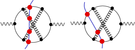
Figure 1: Two cuts of one of the Feynman diagrams that contribute to $e^{+}e^{-}\to{\it hadrons}$.

The contribution ${\cal I}^{(2)}$ to $\cal I$ proportional to $\alpha_{s}^{2}$ can be expressed in terms of cut Feynman diagrams, as in Fig. 1. (In this section, we consider diagrams that do not have self-energy subdiagrams, since self-energy diagrams require a special treatment.) The dots where the parton lines cross the cut represent the function ${\cal S}_{n}$. Each diagram is a three loop diagram, so we have integrations over loop momenta $\vec{l}_{1}$, $\vec{l}_{2}$ and $\vec{l}_{3}$. Eq. (10) lacks an energy conserving delta function, so we have integrations over four energies, which we might take to be loop energies $l_{1}^{0}$, $l_{2}^{0}$ and $l_{3}^{0}$ chosen in the same way as the loop momenta and the energy $l_{0}^{0}$ entering the graph on the vector boson line. We first perform the energy integrations. For the graphs in which four parton lines cross the cut, there are four mass-shell delta functions $\delta(p_{J}^{2})$. These delta functions eliminate the three energy integrals over $l_{1}^{0}$, $l_{2}^{0}$, and $l_{3}^{0}$ as well as the integral over $l_{0}^{0}$. For the graphs in which three parton lines cross the cut, we can eliminate the integration over $l_{0}^{0}$ and two of the $l_{J}^{0}$ integrals. One integral over the energy $E$ in the virtual loop remains. To perform this integration, we close the integration contour in the lower half $E$ plane. This gives a sum of terms obtained from the original integrand by some simple algebraic substitutions in which $E$ is replaced by a location $E_{i}$ of one of the poles in the lower half $E$ plane. Then we do the same thing except that we close the integration contour in the upper half $E$ plane. Finally, we take the average of these results. (For well behaved integrands, these two contributions are the same, but in Coulomb gauge some of the integrands are not so well behaved, as we shall see.)

Having performed the energy integrations, we are left with an integral of the form

$${\cal I}^{(2)}=\sum_{G}\int d\vec{l}_{1}\,d\vec{l}_{2}\,d\vec{l}_{3}\ \sum_{C}\,g(G,C;\vec{l}_{1},\vec{l}_{2},\vec{l}_{3}).$$ (11)

Here there is a sum over graphs $G$ (of which one is shown in Fig. 1) and there is a sum over the possible cuts $C$ of a given graph. The problem of calculating ${\cal I}^{(2)}$ is now set up in a convenient form for calculation.

If we were using the Ellis-Ross-Terrano method for doing next-to-leading order calculations ERT , we would put the sum over cuts outside of the integrals in Eq. (11). For those cuts $C$ that have three partons in the final state, there is a virtual loop. We can arrange that one of the loop momenta, say $\vec{l}_{1}$, goes around this virtual loop. The essence of the Ellis-Ross-Terrano method is to perform the integration over the virtual loop momentum analytically, while the remaining integrations are performed numerically. The integration over the virtual loop momentum is often ultraviolet divergent, but the ultraviolet divergence is easily removed by a renormalization subtraction. The integration is also typically infrared divergent. This divergence is regulated by working in $3-2\epsilon$ space dimensions and then taking $\epsilon\to 0$ while dropping the $1/\epsilon^{n}$ contributions (after proving that they cancel against other contributions). After the $\vec{l}_{1}$ integration has been performed analytically, the integrations over $\vec{l}_{2}$ and $\vec{l}_{3}$ can be performed numerically. For the cuts $C$ that have four partons in the final state, there are also $1/\epsilon^{n}$ infrared divergences. One uses either a “phase space slicing” or a “subtraction” procedure to isolate these divergences, which cancel the $1/\epsilon^{n}$ pieces from the virtual graphs. In the end, we are left with an integral $\int d\vec{l}_{1}\,d\vec{l}_{2}\,d\vec{l}_{3}$ in exactly three space dimensions that can be performed numerically.

In the numerical method, we keep the sum over cuts $C$ inside the integrations. We take care of the ultraviolet divergences by simple renormalization subtractions on the integrand. We make certain deformations on the integration contours so as to keep away from poles of the form $1/[E_{F}-E_{I}\pm i\epsilon]$, where $E_{F}$ is the energy of the final state and $E_{I}$ is the energy of an intermediate state. Then the integrals are all convergent and we calculate them by Monte Carlo numerical integration.

Let us now look at the contour deformation in a little more detail. We denote the momenta $\{\vec{l}_{1},\vec{l}_{2},\vec{l}_{3}\}$ collectively by $l$ whenever we do not need a more detailed description. Thus

$${\cal I}^{(2)}=\sum_{G}\int\!dl\ \sum_{C}\,g(G,C;l).$$ (12)

For cuts $C$ that leave a virtual loop integration, there are singularities in the integrand of the form $E_{F}-E_{I}+i\epsilon$ (or $E_{F}-E_{I}-i\epsilon$ if the loop is in the complex conjugate amplitude to the right of the cut). Here $E_{F}$ is the energy of the final state defined by the cut $C$ and $E_{I}$ is the energy of a possible intermediate state. For the purpose of this review, all we need to know is that $E_{F}-E_{I}=0$ on a surface in the space of $\vec{l}_{1}$ for fixed $\vec{l}_{2}$ and $\vec{l}_{3}$ if we pick $\vec{l}_{1}$ to be the momentum that flows around the virtual loop. These singularities do not create divergences. The Feynman rules provide us with the $i\epsilon$ prescriptions that tell us what to do about the singularities: we should deform the integration contour into the complex $\vec{l}_{1}$ space so as to keep away from them. Thus we write our integral in the form

$${\cal I}^{(2)}=\sum_{G}\int\!dl\ \sum_{C}\,{\cal J}(G,C;l)\,g(G,C;l+i\kappa(G,C;l)).$$ (13)

Here $i\kappa$ is a purely imaginary nine-dimensional vector that we add to the real nine-dimensional vector $l$ to make a complex nine-dimensional vector. The imaginary part $\kappa$ depends on the real part $l$, so that when we integrate over $l$, the complex vector $l+i\kappa$ lies on a surface, the integration contour, that is moved away from the real subspace. When we thus deform the contour, we supply a jacobian ${\cal J}=\det(\partial(l+i\kappa)/\partial l)$. (See Ref. beowulfPRD for details.)

The amount of deformation $\kappa$ depends on the graph $G$ and, more significantly, the cut $C$. For cuts $C$ that leave no virtual loop, each of the momenta $\vec{l}_{1}$, $\vec{l}_{2}$, and $\vec{l}_{3}$ flows through the final state. For practical reasons, we want the final state momenta to be real. Thus we set $\kappa=0$ for cuts $C$ that leave no virtual loop. On the other hand, when the cut $C$ does leave a virtual loop, we choose a non-zero $\kappa$. We must, however, be careful. When $\kappa=0$ there are singularities in $g$ on certain surfaces that correspond to collinear parton momenta. These singularities cancel between $g$ for one cut $C$ and $g$ for another. This cancellation would be destroyed if, for $l$ approaching the collinear singularity, $\kappa=0$ for one of these cuts but not for the other. For this reason, we insist that for all cuts $C$, $\kappa\to 0$ as $l$ approaches one of the collinear singularities. The details can be found in Ref. beowulfPRD . All that is important here is that $\kappa\to 0$ quadratically with the distance to a collinear singularity.

Much has been left out in this brief overview, but we should now have enough background to see what to do in Coulomb gauge. It might seem that all we have to do is use the Feynman rules in Coulomb gauge, but there are some questions associated with the two and three point subdiagrams that need a special analysis. We now turn to that analysis, beginning with a description of a momentum space coordinate system that is useful for the two point subdiagrams.

III Elliptical coordinates

Most of our effort will be devoted to the gluon and quark one loop self-energy diagrams. In these diagrams, we begin by performing the integration over the loop energy by contour integration. This leaves an integration over the loop three-momentum. We will be greatly helped by expressing the components of the loop momentum in terms of three appropriately chosen variables $\{\Delta,x,\phi\}$. These variables are defined by considering, instead of the virtual self-energy graph, the corresponding cut self-energy graph.

Consider an off-shell parton carrying momentum $\bar{q}^{\mu}$ that splits into two partons that carry momenta $k_{\pm}^{\mu}$. Let these two partons be on-shell, $k_{\pm}^{2}=0$. Thus $k_{\pm}^{0}=\omega_{\pm}$ where

$$\omega_{\pm}\equiv|\vec{k}_{\pm}|.$$ (14)

We consider the space-part of $\bar{q}^{\mu}$ to be fixed, and we call it $\vec{q}$, while the energy is determined by energy conservation

$$\bar{q}=(\omega_{+}+\omega_{-},\vec{q}).$$ (15)

We define a loop momentum $\vec{l}$ by

$$\vec{k}_{\pm}={\scriptstyle{1\over 2}}\,\vec{q}\pm\vec{l}.$$ (16)

We will use elliptical coordinates $\{\Delta,x,\phi\}$ defined as follows. First, define ${\cal Q}$ by

$${\cal Q}=|\vec{q}\,|.$$ (17)

Now, define coordinates $\{\Delta,x\}$ by

$$\Delta+1 = {1\over{\cal Q}}\,\left(\omega_{+}+\omega_{-}\right),$$

$$2x-1 = {1\over{\cal Q}}\,\left(\omega_{+}-\omega_{-}\right).$$ (18)

Then

$$0<\Delta,\hskip 28.45274pt0<x<1.$$ (19)

Finally, let $\phi$ be the azimuthal angle of $\vec{l}$ in a coordinate system in which the $z$-axis lies in the direction of $\vec{q}$ and the direction of the $x$-axis is defined arbitrarily. Often, we will want to work in $3-2\epsilon$ space dimensions. In this case, $\phi$ stands for a point on the surface of a unit sphere in $2-2\epsilon$ dimensions, with

$$\int d\phi\equiv S(2-2\epsilon)={2\pi^{1-\epsilon}\over\Gamma(1-\epsilon)}.$$ (20)

The surfaces of constant $\Delta$ are ellipsoids, while the surfaces of constant $x$ are paraboloids that are orthogonal to the constant $\Delta$ surfaces. Both of these surfaces are orthogonal to the surfaces of constant $\phi$.

We note immediately that

$$\bar{q}^{2}=(\omega_{+}+\omega_{-})^{2}-{\cal Q}^{2}={\cal Q}^{2}\left[(\Delta+1)^{2}-1\right]={\cal Q}^{2}\Delta(\Delta+2).$$ (21)

The inverse relation is

$$\Delta=\sqrt{1+\bar{q}^{2}/{\cal Q}^{2}}-1.$$ (22)

It will often be convenient to use $\bar{q}^{2}$ as an independent variable instead of $\Delta$.

The part, $\vec{l}_{T}$, of $\vec{l}$ transverse to $\vec{q}$ is determined by a unit vector in $2-2\epsilon$ dimensions specified by $\phi$ and by the magnitude $|\vec{l}_{T}|$, which is

$$|\vec{l}_{T}|=\sqrt{x(1-x)\,\bar{q}^{2}}.$$ (23)

The component of $\vec{l}$ along $\vec{q}$ is

$$\vec{l}\cdot\vec{q}/{\cal Q}=({\cal Q}/2)\,(1+\Delta)(2x-1).$$ (24)

A straightforward calculation shows that the jacobian of the transformation is given by

$${d^{3-2\epsilon}\vec{l}\over 2\omega_{+}2\omega_{-}}={1\over 8{\cal Q}}\,{1\over 1+\Delta}\,[x(1-x)\,\bar{q}^{2}]^{-\epsilon}d\bar{q}^{2}\,dx\,d^{1-2\epsilon}\phi.$$ (25)

With $\epsilon=0$, the transformation from $\{\Delta,x,\phi\}$ to $\vec{l}$ is

$$\vec{l}=|\vec{l}_{T}|\,\cos\phi\ \vec{n}_{x}+|\vec{l}_{T}|\,\sin\phi\ \vec{n}_{y}+(\vec{l}\cdot\vec{q}/{\cal Q})\,\vec{n}_{z}.$$ (26)

Here $\vec{n}_{z}=\vec{q}/{\cal Q}$, while $\vec{n}_{x}$ and $\vec{n}_{y}$ are two unit vectors orthogonal to each other in the plane orthogonal to $n_{z}$.

IV Structure of graphs with a cut gluon propagator

In this and the following sections, we analyze the gluon propagator. We denote by $n^{\mu}$ a unit vector in the time direction, $n=(1,0,0,0)$. We use Coulomb gauge. Information about the use of Coulomb gauge can be found in Refs. ChristLee and leibrandt . We consider diagrams in which there is zero or one loop in the gluon propagator. Thus we deal with the gluon propagator at orders $\alpha_{s}^{0}$ and $\alpha_{s}^{1}$.

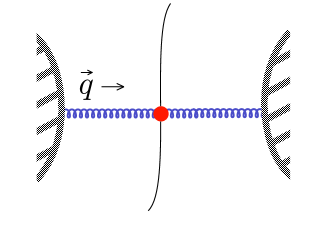
Figure 2: Cut gluon propagator at the Born level.

We will be interested in the factors in the cross section that arise from a cut gluon propagator when the cut propagator is a subgraph of a larger graph. To set the notation, we write the contribution from an order $\alpha_{s}^{0}$ cut propagator, illustrated in Fig. 2, as

$${\cal I}[{\rm Born}]=\int\!d\vec{q}\ {D(q)^{\mu\nu}\over 2{\cal Q}}\,R_{\mu\nu}^{(0)},$$ (27)

where $\vec{q}$ is the three-momentum carried by the propagator, ${\cal Q}\equiv|\vec{q}\,|$, and $q=({\cal Q},\vec{q}\,)$. Then $d\vec{q}/[2{\cal Q}]$ is the standard Lorentz invariant integration over the gluon mass shell. The tensor $R_{\mu\nu}^{(0)}$ denotes the factors associated with the rest of the graph and with the final state measurement function ${\cal S}$; $R_{\mu\nu}^{(0)}$ depends on $\vec{q}$, but this dependence is suppressed in the notation. Finally, $D^{\mu\nu}$ is the numerator function for a bare gluon propagator in Coulomb gauge, which is (for both on-shell and off-shell gluons),

$$D(k)^{\mu\nu}=-g^{\mu\nu}+{1\over\omega^{2}}\left[-k^{\mu}\tilde{k}^{\nu}-\tilde{k}^{\mu}k^{\nu}+k^{\mu}k^{\nu}\right],$$ (28)

where

$$\tilde{k}=(0,\vec{k})$$ (29)

consists of just the $\mu=1,2$ and 3 components of $k^{\mu}$ and where, as in the previous section,

$$\omega=|\vec{k}|=\sqrt{-\tilde{k}^{2}}.$$ (30)

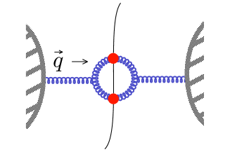
Figure 3: Cut gluon self-energy diagram.

At order $\alpha_{s}^{1}$, we consider a gluon propagator with a one loop self-energy subgraph. We consider three cases. In the first case, the two bare propagators in the self-energy subgraph are cut and the neighboring bare propagators are virtual. This case is illustrated in Fig. 3. We write the contribution of a cut gluon self-energy graph in the form

$${\cal I}[{\rm real}]=\int\!d\vec{q}\ {1\over 4\pi{\cal Q}}\int{d\bar{q}^{2}\over\bar{q}^{2}}\,dx\,d\phi\ {\cal M}_{g}^{\mu\nu}(\bar{q}^{2},x,\phi)\,R_{\mu\nu}(\bar{q}^{2},x,\phi),$$ (31)

ignoring the infrared divergence, which will cancel inside the integral after combining real and virtual contributions in Eq. (IV) below. The integration over the loop momentum $\vec{l}$ has been changed to an integration over $\{\bar{q}^{2},x,\phi\}$ and the factors coming from the cut self-energy graph and its adjacent virtual gluon propagators are included in ${\cal M}/(4\pi{\cal Q}\bar{q}^{2})$. Then $R_{\mu\nu}$ represents the rest of the graph, including the measurement function ${\cal S}$. All of the factors in $R_{\mu\nu}$ depend on the virtuality $\bar{q}^{2}$. The measurement function depends also on $x$ and $\phi$. The dependence of $R_{\mu\nu}$ on $\vec{q}$ is suppressed in the notation. The conventions chosen are such that in Eq. (27) for a cut bare propagator, $R_{\mu\nu}^{(0)}$ is $R_{\mu\nu}(\bar{q}^{2},x,\phi)$ evaluated with $\bar{q}^{2}=0$. Here we use the infrared safety property (2) of the measurement function.

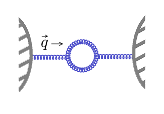
Figure 4: Off-shell virtual gluon self-energy diagram. (This case does not occur in order $\alpha_{s}^{2}$ graphs for $e^{+}e^{-}\to hadrons$, but we consider it as an intermediate step toward analyzing the on-shell gluon self-energy diagram. The analogous off-shell virtual quark self-energy diagram does occur in order $\alpha_{s}^{2}$ graphs for $e^{+}e^{-}\to hadrons$.)

In the second case to be considered below the self-energy loop is entirely virtual and the neighboring bare propagators are not cut, so that the incoming momentum $q$ is off-shell. This case is illustrated in Fig. 4. We consider $q^{2}<0$. In this case, we investigate the quantity

$$F_{g}^{\mu\nu}(q)={1\over q^{2}}\ D(q)_{\alpha}^{\mu}\,\Pi(q)^{\alpha\beta}\,D(q)_{\beta}^{\nu},$$ (32)

where $\Pi^{\alpha\beta}$ is the self-energy function, Eq. (44). There are two factors of $1/q^{2}$ in the propagator function; we include just one of them in the definition of $F_{g}$. We find that $F_{g}^{\mu\nu}(q)$ is given by an integral of the form

$$F_{g}^{\mu\nu}(q)={1\over 2\pi}\int d\bar{q}^{2}\,dx\,d\phi\ {1\over\bar{q}^{2}-q^{2}}\,{W}_{g}^{\mu\nu}(\bar{q}^{2},x,\phi).$$ (33)

The  MS  ultraviolet renormalization is expressed through certain subtraction terms included in $W$.

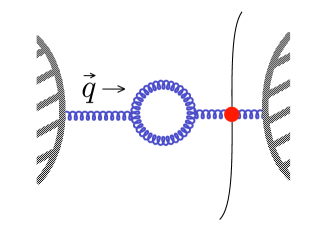
Figure 5: On-shell virtual gluon self-energy diagram.

In the third case, the self-energy loop is entirely virtual and one of the neighboring bare propagators is cut, so that the incoming momentum satisfies $q^{2}=0$. This case is illustrated in Fig. 5. Then we need $F_{g}^{\mu\nu}(q)$ with $q^{2}=0$, which takes the form

$$F_{g}^{\mu\nu}(q)={1\over 2\pi}\int{d\bar{q}^{2}\over\bar{q}^{2}}\,dx\,d\phi\ {\cal W}_{g}^{\mu\nu}(\bar{q}^{2},x,\phi),$$ (34)

where ${\cal W}_{\!g}$ is $W_{\!g}$ with $q^{2}=0$. Again, the integral is infrared divergent, but the divergence will cancel inside the integrand in Eq. (IV). The corresponding contribution to the cross section ${\cal I}$ is

$${\cal I}[{\rm virtual}] = \int\!d\vec{q}\ {1\over 2{\cal Q}}\,F_{g}^{\mu\nu}(q)\,R_{\mu\nu}^{(0)}$$

$$= \int\!d\vec{q}\ {1\over 4\pi{\cal Q}}\int{d\bar{q}^{2}\over\bar{q}^{2}}\,dx\,d\phi\ {\cal W}_{g}^{\mu\nu}(\bar{q}^{2},x,\phi)\,R_{\mu\nu}^{(0)}.$$

We should note that ${\cal I}[{\rm virtual}]$ in Eq. (IV) is the total contribution from the two graphs in which one or the other of the neighboring bare propagators is cut. The contribution from either of these graphs is half of this.

When we add the contributions from graphs with a cut self-energy subdiagram and with a virtual self-energy subdiagram with a cut adjoining bare propagator, we get

$${\cal I}[{\rm real}]+{\cal I}[{\rm virtual}] = \int\!d\vec{q}\ {1\over 4\pi{\cal Q}}\int{d\bar{q}^{2}\over\bar{q}^{2}}\,dx\,d\phi\$$

$$\times\left\{{\cal M}_{g}^{\mu\nu}(\bar{q}^{2},x,\phi)\,R_{\mu\nu}(\bar{q}^{2},x,\phi)+{\cal W}_{g}^{\mu\nu}(\bar{q}^{2},x,\phi)\,R_{\mu\nu}^{(0)}\right\}.$$

As noted above, the integrals of the two terms separately would be infrared divergent and would not make sense by themselves. However, the $\bar{q}^{2}\to 0$ singularities in the integrand in Eq. (IV) cancel, so that the integral is finite and is suitable for calculation by numerical integration.

With this preparation, we are ready to turn to the calculations for the three cases.

V Real gluon self-energy graph

It is straightforward to evaluate the function ${\cal M}_{g}^{\mu\nu}$ defined in Eq. (31). We find

$${\cal M}_{g}^{\mu\nu} = {\alpha_{s}\over 4\pi}\,{1\over 1+\Delta}$$ (37)

$$\times\Biggl{\{}N_{TT}\,D({\cal Q},\vec{q})^{\mu\nu}+N_{tt}\left[{l_{T}^{\mu}l_{T}^{\nu}\over\vec{l}_{T}^{\,2}}-{\textstyle{1\over 2}}D({\cal Q},\vec{q})^{\mu\nu}\right]$$

$$+{\bar{q}^{2}\over{\cal Q}^{2}}N_{EE}\,n^{\mu}n^{\nu}+N_{Et}{\bar{q}\cdot n\over(1+\Delta){\cal Q}^{2}}\left(l_{T}^{\mu}n^{\nu}+n^{\mu}l_{T}^{\nu}\right)\Biggr{\}}.$$

The coefficients $N_{TT},N_{tt},N_{EE},$ and $N_{Et}$ are functions of $\bar{q}^{2}$ and $x$ and are given below. The tensor $D({\cal Q},\vec{q})^{\mu\nu}$ is the numerator (28) for an on-shell gluon, with momentum $q_{\rm os}=({\cal Q},\vec{q})$. In a reference frame in which $\vec{q}$ is aligned with the $z$-axis, the only non-zero components of $D({\cal Q},\vec{q})^{\mu\nu}$ are $D({\cal Q},\vec{q})^{ij}=\delta^{ij}$ with $i,j\in\{1,2\}$. In the second term, using the notation of Sec. III, $l_{T}^{\mu}$ is the vector

$$l_{T}^{0} = 0,$$

$$\vec{l}_{T} = \vec{l}-{\vec{l}\cdot\vec{q}\over{\cal Q}^{2}}\ \vec{q},$$ (38)

or

$$l_{T}^{\mu}=\sqrt{x(1-x)\,\bar{q}^{2}}\left(\cos\phi\,n_{x}^{\mu}+\sin\phi\,n_{y}^{\mu}\right).$$ (39)

Note that this term vanishes if we average over angles $\phi$. The third term gives ${\cal M}^{00}$. It vanishes when $\bar{q}^{2}\to 0$. Finally, the fourth term gives ${\cal M}^{0i}$ and ${\cal M}^{i0}$. Note that it vanishes if we average over angles $\phi$.

We have written Eq. (37) in a more elaborate form than might have seemed necessary: $\bar{q}\cdot n=(1+\Delta)Q$, so the coefficient in the fourth term could have been simplified. The reason for the more elaborate form is as follows. The tensor ${\cal M}_{g}^{\mu\nu}$ is a function of the momenta $\bar{q}^{\mu},k_{+}^{\mu},k_{-}^{\mu}$ carried on the lines of the graph. In the derivation, we have understood that gluons with momenta $k_{+}^{\mu}$ and $k_{-}^{\mu}$ enter the final state. However in a calculation, it might be convenient to use momenta with reversed signs: $\bar{q}^{\mu}\to-\bar{q}^{\mu},k_{+}^{\mu}\to-k_{+}^{\mu},k_{-}^{\mu}\to-k_{-}^{\mu}$. Then the vector $l_{T}^{\mu}$ is also reversed, while $\cal Q$, $\Delta$, and $x$ are unchanged. We have written ${\cal M}_{g}^{\mu\nu}$ in Eq. (37) in a form that is unchanged under this reversal of momenta.

The coefficients are

$$N_{TT} = 2C_{A}\biggl{\{}x(1-x)+{8x(1-x)[1-x(1-x)]\over\bar{q}^{2}/{\cal Q}^{2}+4x(1-x)}$$

$$\hskip 28.45274pt+{16x(1-x)[1-4x(1-x)+2x^{2}(1-x)^{2}]\over[\bar{q}^{2}/{\cal Q}^{2}+4x(1-x)]^{2}}\biggr{\}}$$

$$+N_{F}\biggl{\{}1-2x(1-x)\biggr{\}},$$

$$N_{tt} = 4C_{A}\biggl{\{}x(1-x)-{8x^{2}(1-x)^{2}\over\bar{q}^{2}/{\cal Q}^{2}+4x(1-x)}+{32x^{3}(1-x)^{3}\over[\bar{q}^{2}/{\cal Q}^{2}+4x(1-x)]^{2}}\biggr{\}}$$

$$-4N_{F}x(1-x),$$

$$N_{EE} = C_{A}\biggl{\{}[1-4x(1-x)]-{8x(1-x)[1-4x(1-x)]\over\bar{q}^{2}/{\cal Q}^{2}+4x(1-x)}$$

$$\hskip 28.45274pt+{32x^{2}(1-x)^{2}[1-4x(1-x)]\over[\bar{q}^{2}/{\cal Q}^{2}+4x(1-x)]^{2}}\biggr{\}}$$

$$+4N_{F}x(1-x),$$

$$N_{Et} = 2C_{A}(2x-1)\biggl{\{}-1-{2[1-4x(1-x)]\over\bar{q}^{2}/{\cal Q}^{2}+4x(1-x)}+{16x(1-x)[1-2x(1-x)]\over[\bar{q}^{2}/{\cal Q}^{2}+4x(1-x)]^{2}}\biggr{\}}$$ (40)

$$+2N_{F}(2x-1).$$

(In this paper, we use the standard notation in which $N_{F}$ is the number of quark flavors, $N_{C}$ is the number of colors, $C_{A}=N_{C}$, and $C_{F}=(N_{C}^{2}-1)/(2N_{C})$.)

The behavior of ${\cal M}^{\mu\nu}$ as $\bar{q}^{2}\to 0$ is important. Leaving out the $N_{tt}$ and $N_{Et}$ terms, which average to zero after integrating over angles, we obtain

$${\cal M^{\mu\nu}}\sim D(q)^{\mu\nu}\,{\alpha_{s}\over 2\pi}\left\{{\textstyle{1\over 2}}\,\tilde{P}_{g/g}(x)+N_{F}\tilde{P}_{q/g}(x)\right\},$$ (41)

where

$$\tilde{P}_{q/g}(x) = {\textstyle{1\over 2}}[1-2x(1-x)],$$

$$\tilde{P}_{g/g}(x) = 2C_{A}{[1-x(1-x)]^{2}\over x(1-x)}$$ (42)

are the one loop parton evolution kernels without their $x\to 1$ regulation. Notice that $\tilde{P}_{g/g}(x)$ is singular at $x\to 0$ and $x\to 1$ but that ${\cal M}^{\mu\nu}$ is not singular at these points. The singularities emerge only when we take the $\bar{q}^{2}\to 0$ limit. Also notice that in front of $\tilde{P}_{g/g}(x)$ in Eq. (41) there is a symmetry factor $1/2$, which arises because the two final state gluons in $g\to gg$ are identical.

VI Virtual gluon self-energy graph

In this section, we analyze the virtual gluon self-energy graph at spacelike momentum $q^{\mu}$. We consider the self-energy function $\Pi(q)^{\mu\nu}$. Later, we also consider the quantity

$$F_{g}^{\mu\nu}(q)={1\over q^{2}}\ D(q)_{\mu^{\prime}}^{\mu}\,\Pi(q)^{\mu^{\prime}\nu^{\prime}}\,D(q)_{\nu^{\prime}}^{\nu},$$ (43)

where $D(q)_{\mu^{\prime}}^{\mu}$ is the numerator (28) of the bare gluon propagator. In applications with a cut gluon propagator, as in Fig. 5, one needs $F_{g}^{\mu\nu}(q)$ evaluated with $q^{2}=0$.

We let the momenta of the two partons in the loop be $k_{\pm}^{\mu}$, with $k_{+}^{\mu}+k_{-}^{\mu}=q^{\mu}$. Then the Feynman rules for $\Pi(q)^{\mu\nu}$ give

$$\Pi(q)^{\mu\nu} = ig^{2}\,\tilde{\mu}^{2\epsilon}\int{d^{4-2\epsilon}k_{+}\over(2\pi)^{4-2\epsilon}}\ {1\over(k_{+}^{2}+i\epsilon)(k_{-}^{2}+i\epsilon)}$$ (44)

$$\times\biggl{\{}-{C_{A}\over 2}\,V^{\mu\alpha\beta}(q,-k_{+},-k_{-})\,D_{\alpha\alpha^{\prime}}(k_{+})\,D_{\beta\beta^{\prime}}(k_{-})\,V^{\alpha^{\prime}\beta^{\prime}\nu}(k_{+},k_{-},-q)$$

$$\ \ \ \ +{C_{A}\over 2}\,(\tilde{k}_{+}^{\mu}\tilde{k}_{-}^{\nu}+\tilde{k}_{-}^{\mu}\tilde{k}_{+}^{\nu})\ {k_{+}^{2}k_{-}^{2}\over\omega_{+}^{2}\omega_{-}^{2}}$$

$$\ \ \ \ +{1\over 2}\,N_{F}\,{\rm Tr}\left[\gamma^{\mu}\hbox to0.0pt{/\hss}k_{-}\gamma^{\nu}\hbox to0.0pt{/\hss}k_{+}\right]\biggr{\}}$$

$$-({\rm pole}),$$

where

$$V^{\alpha\beta\gamma}(k_{A},k_{B},k_{C})=g^{\alpha\beta}(k_{A}^{\gamma}-k_{B}^{\gamma})+g^{\beta\gamma}(k_{B}^{\alpha}-k_{C}^{\alpha})+g^{\gamma\alpha}(k_{C}^{\beta}-k_{A}^{\beta}).$$ (45)

Here the first line is for the gluon loop, the second line is for the ghost loop, symmetrized over the two possible momentum labellings, and the third line is for the quark loop. The gluon loop includes a symmetry factor $1/2$. The terms corresponding to gluon and ghost loops contain group factors $C_{A}=3$, while the term corresponding to a quark loop has a factor $N_{F}$ and a color factor $T_{F}=1/2$. We subtract the ultraviolet pole, as required by the  MS  prescription. (The parameter $\tilde{\mu}$ is related to the  MS  scale $\mu$ by $\mu^{2}=4\pi\tilde{\mu}^{2}e^{-\gamma}$.)

We choose a coordinate system in which the $z$-axis is aligned with $\vec{q}$. Then $q=(q^{0},0,0,{\cal Q})$. We assume that $q^{2}<0$. Later we will take the limit $q^{2}\to 0$.

VI.1 The energy integral

We begin by performing the $k_{+}^{0}$ integral. Consider a term in $\Pi^{\mu\nu}$ of the form

$$ig^{2}\,\tilde{\mu}^{2\epsilon}\int{d^{4-2\epsilon}k_{+}\over(2\pi)^{4-2\epsilon}}\ {A\,f(k_{+},k_{-})\over(k_{+}^{2}+i\epsilon)(k_{-}^{2}+i\epsilon)},$$ (46)

where $A$ is a function of $\vec{k}_{+}$ and $\vec{k}_{-}$ but is independent of $k_{+}^{0}$ and $k_{-}^{0}$. We perform the $k_{+}^{0}$ integration, leaving an integral over $\vec{k}_{+}$. Then we change variables to the elliptical coordinates $\{\bar{q}^{2},x,\phi\}$ defined from $\vec{k}_{\pm}$ as in Sec. III, so that our term takes the form

$$-{\alpha_{s}\over 8\pi^{2}}\int d\bar{q}^{2}\,dx\,d^{1-2\epsilon}\!\phi\ \left[x(1-x)\bar{q}^{2}\over 4\pi^{2}\tilde{\mu}^{2}\right]^{-\epsilon}{A\,g(\bar{q}^{2},x,\phi)\over\bar{q}^{2}-q^{2}}.$$ (47)

Thus we will need an integration table that translates $f$ into $g$.

There is, however, a problem. Some of the integrals over $k_{+}^{0}$ are divergent. Thus we need a definition. We elect to perform the integrals over loop energies inside the integrals over loop three-momenta. We calculate these integrals by closing the energy contours in the lower half plane and then calculate them again by closing the contours in the upper half plane. Finally, we average the two results. The radius of the large semicircles that close the contours are always to be big enough to enclose all poles. Thus our prescription is a simple algebraic prescription of adding, with the appropriate signs and a factor 1/2, the residues of all the poles in the complex energy plane. If we apply this prescription in Feynman gauge, then the energy integrations are all convergent and we get the usual answer. In Coulomb gauge, we make this prescription part of the definition of the gauge. The required integral table is given as Table 1.

Table 1: Integral table relating $f$ in Eq. (46) to $g$ in Eq. (47).

$f$	$g$
1	1
$k_{+}^{2}-k_{-}^{2}$	$(q^{2}-\bar{q}^{2})\,\displaystyle{2x-1\over 1+\Delta}$
$k_{+}^{2}+k_{-}^{2}$	$(q^{2}-\bar{q}^{2})$
$(k_{+}^{2}-k_{-}^{2})^{2}$	$(q^{2}-\bar{q}^{2})\,(q^{2}+4{\cal Q}^{2}x(1-x))$
$(k_{+}^{2})^{2}-(k_{-}^{2})^{2}$	$(q^{2}-\bar{q}^{2})^{2}\ \displaystyle{2x-1\over 1+\Delta}$
$k_{+}^{2}k_{-}^{2}$	$0$

Of these integrals, the most divergent is that for $f=k_{+}^{2}k_{-}^{2}$. There are no poles in the complex loop-energy plane, so we have

$$\int dE=0.$$ (48)

One might expect that if the self-energy diagram is embedded in a larger diagram as part of a gauge invariant calculation, then an $\int\!dE$ contribution from some other virtual loop diagram would cancel this contribution. However, so far as we can see, this does not happen. Specifically, the gluon-quark-antiquark one loop three point function does not have an $\int\!dE$ divergence. Instead, we look to the coefficient of $\int\!dE$. This coefficient is independent of $q^{2}$ and is proportional to the integral

$$\tilde{\mu}^{2\epsilon}\int{d^{3-2\epsilon}\vec{k}_{+}\over(2\pi)^{3-2\epsilon}}\left\{{1\over\vec{k}_{+}^{2}}+{1\over\vec{k}_{-}^{2}}\right\}.$$ (49)

This integral vanishes in dimensional regulation for any $\epsilon$. Thus we have an ambiguous contribution of infinity times zero and we find it sensible that the contour integration prescription given above instructs us to discard this contribution.

The integral for $f=(k_{+}^{2})^{2}-(k_{-}^{2})^{2}$ is logarithmically divergent and can be obtained from the simple integral

$$\int dE\ {E\over E^{2}-M^{2}+i\epsilon}=0.$$ (50)

Zero is a sensible result for this integral since the integrand is odd under $E\to-E$. In our prescription, we get $-i\pi$ when we close the contour in the lower half plane and $+i\pi$ when we close the contour in the upper half plane. Averaging these two results give zero.

Our prescription may be compared to that of Leibbrandt and Williams leibrandt . In that prescription, one imagines that the loop energy is integrated over the imaginary axis and that the integration is performed in $1-2\beta$ dimensions. This prescription gives the same result as the one adopted here: the integral in Eq. (48) becomes $\int d^{1-2\beta}\vec{k}$, which vanishes because it has no scale, while the integral in Eq. (50) becomes $\int d^{1-2\beta}\vec{k}\ \vec{k}\cdot\vec{n}/(\vec{k}^{2}+M^{2}+i\epsilon)$, which vanishes because it is odd under $\vec{k}\cdot\vec{n}\to-\vec{k}\cdot\vec{n}$.

VI.2 Components needed

We will calculate the individual components of $\Pi(q)^{\mu\nu}$ that we need in the coordinate frame with $q=(q^{0},0,0,{\cal Q})$. Since $D(q)^{\mu}_{3}=D(q)^{\nu}_{3}=0$, we need not consider the components $\Pi(q)^{3\nu}$ or $\Pi(q)^{\mu 3}$. In addition, $\Pi(q)^{0i}=\Pi(q)^{i0}=0$ for $i\in\{1,2\}$ because of rotational symmetry. Thus what we need are $\Pi(q)^{00}$ and $\Pi(q)^{ij}$ for $i,j\in\{1,2\}$. We define

$$\Pi(q)^{ij} = q^{2}A_{T}(q^{2})\,\delta^{ij},\hskip 28.45274pti,j\in\{1,2\},$$

$$\Pi(q)^{00} = {\cal Q}^{2}A_{E}(q^{2}).$$ (51)

We turn first to $A_{T}(q)$.

VI.3 Transverse components

We evaluate $A_{T}(q^{2})$ using the integrals in Table 1 and find

$$A_{T}(q^{2}) = -{\alpha_{s}\over 8\pi^{2}}\int d\bar{q}^{2}\,dx\,d^{1-2\epsilon}\!\phi\ \left[x(1-x)\bar{q}^{2}\over 4\pi^{2}\tilde{\mu}^{2}\right]^{-\epsilon}{1\over\bar{q}^{2}-q^{2}}\sum_{J=0}^{2}\ {A^{\prime\prime}_{T,J}\over[\bar{q}^{2}/{\cal Q}^{2}+4x(1-x)]^{J}}$$ (52)

$$-({\rm pole}),$$

where

$$A^{\prime\prime}_{T,0} = C_{A}\,{1\over q^{2}}\biggl{\{}-\bar{q}^{2}/2-3q^{2}/2-4\,{\cal Q}^{2}+2\bar{q}^{2}\,x(1-x)+24\,{\cal Q}^{2}\,x(1-x)$$

$$+{x(1-x)\over(1-\epsilon)}\Bigl{[}\bar{q}^{2}+4\,{\cal Q}^{2}+3\,q^{2}-20\,{\cal Q}^{2}\,x(1-x)\Bigr{]}\biggr{\}}$$

$$-N_{F}\,{1\over q^{2}}\biggl{\{}-\bar{q}^{2}+{x(1-x)\over(1-\epsilon)}\ 2\bar{q}^{2}\biggr{\}},$$

$$A^{\prime\prime}_{T,1} = C_{A}\,{1\over q^{2}}\biggl{\{}4\,q^{2}+2\,({q^{2}})^{2}/{\cal Q}^{2}+48\,{\cal Q}^{2}\,x(1-x)-224\,{\cal Q}^{2}\,[x(1-x)]^{2}$$

$$+\frac{x(1-x)}{(1-\epsilon)}\Bigl{[}-4\,q^{2}-4\,(q^{2})^{2}/{\cal Q}^{2}-32\,{\cal Q}^{2}\,{x(1-x)}$$

$$\ \ \ -28\,q^{2}\,{x(1-x)}+144\,{\cal Q}^{2}\,[x(1-x)]^{2}\Bigr{]}\biggr{\}},$$

$$A^{\prime\prime}_{T,2} = C_{A}\,{1\over q^{2}}\biggl{\{}-128\,{\cal Q}^{2}\,[x(1-x)]^{2}+512\,{\cal Q}^{2}\,[x(1-x)]^{3}$$ (53)

$$+\frac{[x(1-x)]^{2}}{(1-\epsilon)}\Bigl{[}16\,q^{2}+16\,(q^{2})^{2}/{\cal Q}^{2}+64\,{\cal Q}^{2}\,{x(1-x)}$$

$$+64\,q^{2}\,{x(1-x)}-256\,{\cal Q}^{2}\,[x(1-x)]^{2}\Bigr{]}\biggr{\}}.$$

As indicated by the notation, we expect that $q^{2}A_{T}(q^{2})$ vanishes at $q^{2}=0$, but it is not evident from the form above that it does so. Nevertheless, explicit analytical integration shows that $q^{2}A_{T}(q^{2})=0$ at $q^{2}=0$ for any $\epsilon$. In order to get a form in which the vanishing of $q^{2}A_{T}(q^{2})$ at $q^{2}=0$ is manifest, we simply subtract $q^{2}A_{T}(q^{2})$ at $q^{2}=0$, which is zero, from $q^{2}A_{T}(q^{2})$. Then $A_{T}(q^{2})$ still has the form (52) but with new coefficients $A^{\prime}_{T,J}$:

$$A^{\prime}_{T,0} = 2\,C_{A}\biggl{\{}-1+x(1-x)+{2x(1-x)\over(1-\epsilon)}\biggr{\}}+N_{F}\biggl{\{}1-{2x(1-x)\over(1-\epsilon)}\biggr{\}},$$

$$A^{\prime}_{T,1} = 2\,C_{A}\biggl{\{}q^{2}/{\cal Q}^{2}+12x(1-x)-\frac{2x(1-x)}{(1-\epsilon)}\Bigl{[}q^{2}/{\cal Q}^{2}+12x(1-x)\Bigr{]}\biggr{\}},$$

$$A^{\prime}_{T,2} = 16\,C_{A}\,x(1-x)\biggl{\{}2-8x(1-x)+\frac{x(1-x)}{(1-\epsilon)}\Bigl{[}q^{2}/{\cal Q}^{2}+8x(1-x)\Bigr{]}\biggr{\}}.$$ (54)

We now examine the ultraviolet renormalization of $A_{T}(q^{2})$. Define

$$\Delta A_{T}(q^{2}) = {\alpha_{s}\over 8\pi^{2}}\int d\bar{q}^{2}\,dx\,d^{1-2\epsilon}\phi\left[x(1-x)\bar{q}^{2}\over 4\pi^{2}\tilde{\mu}^{2}\right]^{-\epsilon}$$ (55)

$$\times\left\{{-2C_{A}+N_{F}\over\bar{q}^{2}+e^{\lambda_{1}}\mu^{2}}+x(1-x){2C_{A}\over\bar{q}^{2}+e^{\lambda_{2}}\mu^{2}}+{x(1-x)\over 1-\epsilon}\,{4C_{A}-2N_{F}\over\bar{q}^{2}+e^{\lambda_{3}}\mu^{2}}\right\}$$

$$-({\rm pole}).$$

Here $\mu^{2}=4\pi\tilde{\mu}^{2}\,e^{-\gamma}$ is the  MS  scale, $\gamma=0.577\dots$ is the Euler constant, and $\lambda_{1}$, $\lambda_{2}$, and $\lambda_{3}$ are parameters that we will adjust. The integrand in $\Delta A_{T}$ matches that of $A_{T}$ when $\bar{q}^{2}\to\infty$ but it has the opposite sign, so if we add $\Delta A_{T}$ to $A_{T}$, we will obtain an ultraviolet convergent integral. Furthermore, since the integrands match for $\bar{q}^{2}\to\infty$, the ultraviolet pole terms that are included in the definitions are opposite and will cancel in the sum $A_{T}+\Delta A_{T}$. We can easily perform the integral:

$$\Delta A_{T}(q^{2}) = {\alpha_{s}\over 4\pi}\,\Gamma(\epsilon)\,e^{\gamma\epsilon}\biggl{\{}-(2C_{A}-N_{F}){\Gamma(1-\epsilon)^{2}\over\Gamma(2-2\epsilon)}\ e^{-\lambda_{1}\epsilon}+2C_{A}{\Gamma(2-\epsilon)^{2}\over\Gamma(4-2\epsilon)}e^{-\lambda_{2}\epsilon}$$ (56)

$$+(4C_{A}-2N_{F})\,{\Gamma(2-\epsilon)^{2}\over(1-\epsilon)\Gamma(4-2\epsilon)}e^{-\lambda_{3}\epsilon}\biggr{\}}-({\rm pole})$$

$$= {\alpha_{s}\over 4\pi}\left\{-(2C_{A}-N_{F})\,\left(2-\lambda_{1}\right)+{2C_{A}\over 6}\,\left({5\over 3}-\lambda_{2}\right)+{4C_{A}-2N_{F}\over 6}\,\left({8\over 3}-\lambda_{3}\right)\right\}$$

$$+{\cal O}(\epsilon)\rule{0.0pt}{15.0pt}.$$

We set

$$\lambda_{1}=2,\hskip 28.45274pt\lambda_{2}={5\over 3},\hskip 28.45274pt\lambda_{3}={8\over 3}.$$ (57)

Then

$$\Delta A_{T}(q^{2})=0+{\cal O}(\epsilon).$$ (58)

Since $\Delta A_{T}$ is zero, we can add it to $A_{T}$ to obtain, after setting $\epsilon$ to zero,

$$A_{T}(q^{2})=-{\alpha_{s}\over 8\pi^{2}}\int d\bar{q}^{2}\,dx\,d\phi\ {1\over\bar{q}^{2}-q^{2}}\sum_{J=0}^{2}\ {A_{T,J}\over[\bar{q}^{2}/{\cal Q}^{2}+4x(1-x)]^{J}},$$ (59)

where

$$A_{T,0} = -(2C_{A}-N_{F})\,{q^{2}+e^{2}\mu^{2}\over\bar{q}^{2}+e^{2}\mu^{2}}\,+2C_{A}\,x(1-x)\,{q^{2}+e^{5/3}\mu^{2}\over\bar{q}^{2}+e^{5/3}\mu^{2}}$$

$$+(4C_{A}-2N_{F})\,x(1-x)\,{q^{2}+e^{8/3}\mu^{2}\over\bar{q}^{2}+e^{8/3}\mu^{2}}\ ,$$

$$A_{T,1} = 2C_{A}\biggl{\{}q^{2}/{\cal Q}^{2}+12x(1-x)-{2x(1-x)}\Bigl{[}q^{2}/{\cal Q}^{2}+12x(1-x)\Bigr{]}\biggr{\}},$$

$$A_{T,2} = 16C_{A}\,x(1-x)\biggl{\{}2-8x(1-x)+{x(1-x)}\Bigl{[}q^{2}/{\cal Q}^{2}+8x(1-x)\Bigr{]}\biggr{\}}.$$ (60)

VI.4 Timelike components

We evaluate $A_{E}(q^{2})$ using the integrals in Table 1 and find

$$A_{E}(q^{2}) = -{\alpha_{s}\over 8\pi^{2}}\int d\bar{q}^{2}\,dx\,d^{1-2\epsilon}\!\phi\ \left[x(1-x)\bar{q}^{2}\over 4\pi^{2}\tilde{\mu}^{2}\right]^{-\epsilon}{1\over\bar{q}^{2}-q^{2}}\sum_{J=0}^{2}\ {A^{\prime\prime}_{E,J}\over[\bar{q}^{2}/{\cal Q}^{2}+4x(1-x)]^{J}}$$ (61)

$$-({\rm pole}),$$

where

$$A^{\prime\prime}_{E,0} = C_{A}\biggl{\{}-24x(1-x)+(1-\epsilon)\left[(q^{2}-\bar{q}^{2})/{\cal Q}^{2}+1-4x(1-x)\right]\biggr{\}}+4N_{F}\,x(1-x),$$

$$A^{\prime\prime}_{E,1} = 8C_{A}\,x(1-x)\biggl{\{}-1+3q^{2}/{\cal Q}^{2}+28x(1-x)\biggr{\}},$$

$$A^{\prime\prime}_{E,2} = 32C_{A}\,[x(1-x)]^{2}\biggl{\{}1-3q^{2}/{\cal Q}^{2}-16x(1-x)\biggr{\}}.$$ (62)

We note that $A^{\prime\prime}_{E,0}$ contains a term $C_{A}(1-\epsilon)(q^{2}-\bar{q}^{2})/{\cal Q}^{2}$. This term is undesirable for numerical integration because it leads to a quadratically ultraviolet divergent integral. Furthermore, this term gives a contribution to the integral that vanishes for all $\epsilon$. For these reasons, we eliminate the term. Then $A_{E}(q^{2})$ still has the form (61) but with new coefficients $A^{\prime}_{E,J}$:

$$A^{\prime}_{E,0} = C_{A}\biggl{\{}-24x(1-x)+(1-\epsilon)\left[1-4x(1-x)\right]\biggr{\}}+4N_{F}\,x(1-x),$$

$$A^{\prime}_{E,1} = 8\,C_{A}\,x(1-x)\biggl{\{}-1+3q^{2}/{\cal Q}^{2}+28\,x(1-x)\biggr{\}},$$

$$A^{\prime}_{E,2} = 32\,C_{A}\,[x(1-x)]^{2}\biggl{\{}1-3\,q^{2}/{\cal Q}^{2}-16\,x(1-x)\biggr{\}}.$$ (63)

We now examine the ultraviolet renormalization of $A_{E}(q^{2})$. Define

$$\Delta A_{E}(q^{2}) = {\alpha_{s}\over 8\pi^{2}}\int d\bar{q}^{2}\,dx\,d^{1-2\epsilon}\phi\left[x(1-x)\bar{q}^{2}\over 4\pi^{2}\tilde{\mu}^{2}\right]^{-\epsilon}$$ (64)

$$\times\left\{(1-\epsilon)\,{C_{A}\over\bar{q}^{2}+e^{\lambda_{4}}\mu^{2}}-x(1-x)\,{24C_{A}-4N_{F}\over\bar{q}^{2}+e^{\lambda_{5}}\mu^{2}}-x(1-x)(1-\epsilon)\,{4C_{A}\over\bar{q}^{2}+e^{\lambda_{6}}\mu^{2}}\right\}$$

$$-({\rm pole}).$$

Here as before $\mu^{2}=4\pi\tilde{\mu}^{2}\,e^{-\gamma}$ is the  MS  scale and $\lambda_{4}$, $\lambda_{5}$, and $\lambda_{6}$ are parameters that we will adjust. The integrand in $\Delta A_{E}$ matches that of $A_{E}$ when $\bar{q}^{2}\to\infty$ but it has the opposite sign, so if we add $\Delta A_{E}$ to $A_{E}$, we will obtain an ultraviolet convergent integral. Furthermore, since the integrands match for $\bar{q}^{2}\to\infty$, the ultraviolet pole terms that are included in the definitions are opposite and will cancel in the sum $A_{E}+\Delta A_{E}$. We can easily perform the integration:

$$\Delta A_{E}(q^{2}) = {\alpha_{s}\over 4\pi}\,\Gamma(\epsilon)\,e^{\gamma\epsilon}\biggl{\{}C_{A}\,{(1-\epsilon)\Gamma(1-\epsilon)^{2}\over\Gamma(2-2\epsilon)}\ e^{-\lambda_{4}\epsilon}$$ (65)

$$-(24C_{A}-4N_{F})\,{\Gamma(2-\epsilon)^{2}\over\Gamma(4-2\epsilon)}e^{-\lambda_{5}\epsilon}-4C_{A}\,{(1-\epsilon)\Gamma(2-\epsilon)^{2}\over\Gamma(4-2\epsilon)}e^{-\lambda_{6}\epsilon}\biggr{\}}-({\rm pole})$$

$$= {\alpha_{s}\over 4\pi}\left\{C_{A}\,(1-\lambda_{4})-(24C_{A}-4N_{F})\,{1\over 6}\,({5\over 3}-\lambda_{5})-4C_{A}\,{1\over 6}\,({2\over 3}-\lambda_{6})\right\}$$

$$+{\cal O}(\epsilon).\rule{0.0pt}{15.0pt}$$

We set

$$\lambda_{4}=1,\hskip 28.45274pt\lambda_{5}={5\over 3},\hskip 28.45274pt\lambda_{6}={2\over 3}.$$ (66)

Then

$$\Delta A_{E}(q^{2})=0+{\cal O}(\epsilon).$$ (67)

Since $\Delta A_{E}$ is zero, we can add it to $A_{E}$ to obtain, after setting $\epsilon$ to zero,

$$A_{E}(q^{2})=-{\alpha_{s}\over 8\pi^{2}}\int d\bar{q}^{2}\,dx\,d\phi\ {1\over\bar{q}^{2}-q^{2}}\sum_{J=0}^{2}\ {A_{E,J}\over[\bar{q}^{2}/{\cal Q}^{2}+4x(1-x)]^{J}},$$ (68)

where

$$A_{E,0} = C_{A}\ {q^{2}+e^{1}\mu^{2}\over\bar{q}^{2}+e^{1}\mu^{2}}\,-(24C_{A}-4\,N_{F})\,x(1-x)\,{q^{2}+e^{5/3}\mu^{2}\over\bar{q}^{2}+e^{5/3}\mu^{2}}-4C_{A}\,x(1-x)\,{q^{2}+e^{2/3}\mu^{2}\over\bar{q}^{2}+e^{2/3}\mu^{2}}\ ,$$

$$A_{E,1} = 8\,C_{A}\,x(1-x)\biggl{\{}-1+3q^{2}/{\cal Q}^{2}+28\,x(1-x)\biggr{\}},$$

$$A_{E,2} = 32\,C_{A}\,[x(1-x)]^{2}\biggl{\{}1-3\,q^{2}/{\cal Q}^{2}-16\,x(1-x)\biggr{\}}.$$ (69)

VI.5 The tensor $F_{g}^{\mu\nu}$

We can assemble this information to obtain $F_{g}^{\mu\nu}(q)$ defined in Eq. (43). With $\vec{q}$ directed along the $z$ axis, the only non-zero components of $F_{g}^{\mu\nu}$ are $F_{g}^{00}$ and $F_{g}^{ij}$ for $i,j\in\{1,2\}$:

$$F_{g}^{ij}(q) = A_{T}(q^{2})\,\delta^{ij},\hskip 28.45274pti,j\in\{1,2\},$$

$$F_{g}^{00}(q) = {q^{2}\over{\cal Q}^{2}}\,A_{E}(q^{2}).$$ (70)

We can write this in a form valid for any direction of $\vec{q}$ as

$$F_{g}^{\mu\nu}(q)=D(q)^{\mu\nu}A_{T}(q^{2})+n^{\mu}n^{\nu}{q^{2}\over{\cal Q}^{2}}\,\left[A_{E}(q^{2})-A_{T}(q^{2})\right].$$ (71)

Here $D(q)^{\mu\nu}$ is the numerator for the bare gluon propagator, Eq. (28), with $D^{00}=q^{2}/{\cal Q}^{2}$. Note that this result is physically sensible. The complete one loop contribution to the gluon propagator is $F^{\mu\nu}(q)/q^{2}$. It has a simple pole times logarithms at $q^{2}=0$. The pole multiplies a projection onto transverse polarizations.

VI.6 ${W}_{g}^{\mu\nu}$ and its supplementary terms

From Eq. (71) we obtain the tensor ${W}_{g}^{\mu\nu}$ defined in Eq. (33),

$${W}_{g}^{\mu\nu} = -{\alpha_{s}\over 4\pi}\ D(q)^{\mu\nu}\sum_{J}{A_{T,J}\over[\bar{q}^{2}/{\cal Q}^{2}+4x(1-x)]^{J}}$$ (72)

$$-{\alpha_{s}\over 4\pi}\ n^{\mu}n^{\nu}{q^{2}\over{\cal Q}^{2}}\sum_{J}{A_{E,J}-A_{T,J}\over[\bar{q}^{2}/{\cal Q}^{2}+4x(1-x)]^{J}}.$$

We can now set $q^{2}$ to 0 in ${W}_{g}^{\mu\nu}$ to obtain ${\cal W}_{g}^{\mu\nu}$. We have

$${\cal W}_{g}^{\mu\nu}[{\rm simple}]=-{\alpha_{s}\over 2\pi}\ D(q)^{\mu\nu}\,{\cal P}_{\!g}(\bar{q}^{2},x),$$ (73)

where

$${\cal P}_{\!g}(\bar{q}^{2},x)={1\over 2}\sum_{J}{A_{T,J}\over[\bar{q}^{2}/{\cal Q}^{2}+4x(1-x)]^{J}}.$$ (74)

Here the coefficients $A_{T,J}$ from Eq. (60) are evaluated with $q^{2}=0$.

We see immediately that there will be a numerical problem for the cancellation of ${\cal W}_{g}^{\mu\nu}$ with ${\cal M}_{g}^{\mu\nu}$ at the small $\bar{q}^{2}$ endpoint of the integration (IV). In Eq. (37) for ${\cal M}_{g}^{\mu\nu}$, there are terms with four tensor structures. There is a good cancellation for the $D(q)^{\mu\nu}$ structure (as we will see below) and the $n^{\mu}n^{\nu}$ structure is not important because it multiplies a factor $\bar{q}^{2}$ in Eq. (37) for ${\cal M}_{g}^{\mu\nu}$. For the other two terms, involving $l_{T}^{\mu}$, the singularity in ${\cal M}_{g}^{\mu\nu}$ will vanish if we integrate over the angle $\phi$ of $l_{T}^{\mu}$ before letting $\bar{q}^{2}$ become small. However, this is not suitable for a numerical integration. Therefore, we modify ${\cal W}_{g}^{\mu\nu}$ to

$${\cal W}_{g}^{\mu\nu} = -{\alpha_{s}\over 2\pi}\ D(q)^{\mu\nu}\,{\cal P}_{\!g}(\bar{q}^{2},x)$$ (75)

$$-{\alpha_{s}\over 4\pi}\left[{l_{T}^{\mu}l_{T}^{\nu}\over\vec{l}_{T}^{\,2}}-{\textstyle{1\over 2}}D(q)^{\mu\nu}\right]\,{N_{tt}\over(1+\bar{q}^{2}/{\cal Q}^{2})}$$

$$-{\alpha_{s}\over 4\pi}{q\cdot n\over(1+\Delta){\cal Q}^{2}}\left(l_{T}^{\mu}n^{\nu}+n^{\mu}l_{T}^{\nu}\right)\,{N_{Et}\over(1+\bar{q}^{2}/{\cal Q}^{2})}\ ,$$

where $N_{tt}$ and $N_{Et}$ are functions of $\bar{q}^{2}$ and $x$ and are given in Eq. (40). The integral of the extra terms vanishes (because the integration over $\phi$ gives zero), so we are adding zero to $F_{g}^{\mu\nu}$. However the cancellation in Eq. (IV) now works point by point in $\{\bar{q}^{2},x,\phi\}$ space. We have inserted factors $1/(1+\bar{q}^{2}/{\cal Q}^{2})$ in the extra terms so as not to create problems at $\bar{q}^{2}\to\infty$ at the same time as we were alleviating problems at $\bar{q}^{2}\to 0$. As in Eq. (37), we have written ${\cal W}_{g}^{\mu\nu}$ in Eq. (75) in a form that is invariant under the replacements $q^{\mu}\to-q^{\mu},l^{\mu}\to-l^{\mu}$.

Let us examine the cancellation for $\bar{q}^{2}\to 0$ in Eq. (IV). The terms with tensor structures involving $l_{T}^{\mu}$ cancel the corresponding terms in ${\cal M}_{g}^{\mu\nu}$ by construction. For the $D(q)^{\mu\nu}$ term, the $\bar{q}^{2}\to 0$ limit is

$${\cal W}_{g}^{\mu\nu}\sim-{\alpha_{s}\over 2\pi}\ D(q)^{\mu\nu}\,{\cal P}_{\!g}(0,x).$$ (76)

We find for ${\cal P}_{\!g}(\bar{q}^{2},x)$ at $\bar{q}^{2}=0$,

$${\cal P}_{\!g}(0,x)={\textstyle{1\over 2}}\,\tilde{P}_{g/g}(x)+N_{F}\tilde{P}_{q/g}(x),$$ (77)

where the parton evolution kernels $\tilde{P}_{g/g}(x)$ and $\tilde{P}_{q/g}(x)$ are given in Eq. (42). Using Eq. (41), we see that this is just the behavior we needed to make the cancellation work.

VII Structure of graphs with a cut quark propagator

In this and the following sections, we analyze the quark propagator in Coulomb gauge. To set the notation, we write the contribution from an order $\alpha_{s}^{0}$ cut propagator as

$${\cal I}[{\rm Born}]=\int\!d\vec{q}\ {\rm Tr}\left\{{\hbox to0.0pt{/\hss}q\over 2{\cal Q}}\,R_{0}\right\},$$ (78)

where, as in Sec. IV, $R_{0}$ denotes the factors associated with the rest of the graph and with the final state measurement function ${\cal S}$. The function $R_{0}$ carries hidden Dirac indices and there is a trace over the Dirac indices of $\hbox to0.0pt{/\hss}q\,R_{0}$.

Following the notation employed for the gluon propagator, we write the contribution of a cut quark self-energy graph as

$${\cal I}[{\rm real}]=\int\!d\vec{q}\ {\rm Tr}\left\{{1\over 4\pi{\cal Q}}\int{d\bar{q}^{2}\over\bar{q}^{2}}\,dx\,d\phi\ {\cal M}_{q}(\bar{q}^{2},x,\phi)\,R(\bar{q}^{2},x,\phi)\right\}.$$ (79)

With this notation, the contribution from the virtual self-energy graph with an adjoining cut bare propagator is

$${\cal I}[{\rm virtual}]=\int\!d\vec{q}\ {\rm Tr}\left\{{1\over 2{\cal Q}}\,F_{q}(q)\,R_{0}\right\},$$ (80)

where

$$F_{q}(q)={\hbox to0.0pt{/\hss}q\Sigma(q)\hbox to0.0pt{/\hss}q\over q^{2}}.$$ (81)

We should note that ${\cal I}[{\rm virtual}]$ in Eq. (80) is the total contribution from the two graphs in which one or the other of the neighboring bare propagators is cut. The contribution from either of these graphs is half of this.

If both of the adjoining bare propagators are uncut, the corresponding expression is

$${\cal I}[{\rm all\ uncut}]=\int\!d^{4}q\ {\rm Tr}\left\{{1\over q^{2}}\,F_{q}(q)\,R(q^{2})\right\},$$ (82)

where, here, $R$ is defined so that the corresponding Born contribution is $R(q^{2})\hbox to0.0pt{/\hss}q/q^{2}$.

We investigate $F_{q}(q)$ in the following section. First, we take $q^{2}<0$. We write $F_{q}(q)$ as an integral

$$F_{q}(q)={1\over 2\pi}\int d\bar{q}^{2}\,dx\,d\phi\ {1\over\bar{q}^{2}-q^{2}}\,{W}_{q}(\bar{q}^{2},x,\phi).$$ (83)

Then the contribution to the graph when the adjoining bare propagators are uncut is

$${\cal I}[{\rm all\ uncut}]=\int\!d^{4}q\ {\rm Tr}\left\{{1\over 2\pi\,q^{2}}\int d\bar{q}^{2}\,dx\,d\phi\ {1\over\bar{q}^{2}-q^{2}}\,{W}_{q}(\bar{q}^{2},x,\phi)\,R(q^{2})\right\}.$$ (84)

Now, taking $q^{2}$ to zero, we write $F_{q}(q)$ as

$$F_{q}(q)={1\over 2\pi}\int{d\bar{q}^{2}\over\bar{q}^{2}}\,dx\,d\phi\ {\cal W}_{q}(\bar{q}^{2},x,\phi),$$ (85)

where ${\cal W}_{\!q}$ is $W_{\!q}$ with $q^{2}=0$. Then

$${\cal I}[{\rm real}]+{\cal I}[{\rm virtual}] = \int\!d\vec{q}\ {\rm Tr}\biggl{\{}{1\over 4\pi{\cal Q}}\int{d\bar{q}^{2}\over\bar{q}^{2}}\,dx\,d\phi\$$

$$\times\left[{\cal M}_{q}(\bar{q}^{2},x,\phi)\,R(\bar{q}^{2},x,\phi)+{\cal W}_{q}(\bar{q}^{2},x,\phi)\,R_{0}\right]\biggr{\}}.$$

As we shall see, the $\bar{q}^{2}\to 0$ singularities in the integrand in Eq. (VII) cancel, so that the integral is finite and is suitable for calculation by numerical integration.

VIII Real quark self-energy graph

It is straightforward to evaluate the function ${\cal M}_{q}$ defined in Eq. (79). We find

$${\cal M}_{q}={\alpha_{s}\over 4\pi}\,{1\over 1+\Delta}\left\{N_{L}\,\hbox to0.0pt{/\hss}q_{\rm os}+N_{E}\,\Delta\ n\cdot q_{\rm os}\,\hbox to0.0pt{/\hss}n+N_{t}\,\hbox to0.0pt{/\hss}l_{T}\right\}.$$ (87)

The coefficients $N_{L},N_{E}$, and $N_{t}$ are functions of $\bar{q}^{2}$ and $x$ and are given below. The momentum in the first two terms is $q_{\rm os}=(\bar{q}^{0}/(1+\Delta),\vec{q})=((k_{+}^{0}+k_{-}^{0})/(1+\Delta),\vec{q})$ so that $q_{\rm os}^{2}=0$. In the third term, using the notation of Sec. III, $l_{T}^{\mu}$ is the part of the loop momentum orthogonal to $n^{\mu}$ and $q_{\rm os}^{\mu}$. Note that this term vanishes if we average over angles $\phi$.

The coefficients are

$$N_{L} = C_{F}\Biggl{\{}12x(1-x)+(2x-1)(2x+\Delta)$$

$$\ \ \ \ \ -{16x(1-x)(2x-1)\over 2x+\Delta}+{16x(1-x)[1-2x(1-x)]\over(2x+\Delta)^{2}}\Biggr{\}},$$

$$N_{E} = 2C_{F}\,{(1-x)(4x^{2}+\Delta^{2})\over(2x+\Delta)^{2}}\ ,$$

$$N_{t} = 2C_{F}\left\{1-{2(2x-1)\over 2x+\Delta}-{8x(1-x)\over(2x+\Delta)^{2}}\right\}.$$ (88)

The behavior of ${\cal W}_{q}^{\mu\nu}$ as $\bar{q}^{2}\to 0$ is important. Leaving out the $\hbox to0.0pt{/\hss}l_{T}$ term since $l_{T}\to 0$ as $\bar{q}^{2}\to 0$, we obtain

$${\cal M}_{q}^{\mu\nu}\sim\hbox to0.0pt{/\hss}q\,{\alpha_{s}\over 2\pi}\ \tilde{P}_{g/q}(x),$$ (89)

where

$$\tilde{P}_{g/q}(x)=C_{F}\,{1+(1-x)^{2}\over x}$$ (90)

is the one loop parton evolution kernel for $q\to g$. Notice that $\tilde{P}_{q/g}(x)$ is singular at $x\to 0$ but that ${\cal M}_{q}$ is not singular at this point. The singularity emerges only when we take the $\bar{q}^{2}\to 0$ limit.

For the integrand of a cut antiquark self-energy graph, we have ${\cal M}_{\bar{q}}=-{\cal M}_{q}$. We note that ${\cal M}_{q}$ in Eq. (87) is odd under the interchange $\bar{q}^{\mu}\to-\bar{q}^{\mu}$, $k_{+}^{\mu}\to-k_{+}^{\mu}$, $k_{-}^{\mu}\to-k_{-}^{\mu}$ (so that also $l^{\mu}\to-l^{\mu}$). Thus for an antiquark, we can simply use Eq. (87) and reverse the momenta, so that $\bar{q}^{\mu}$ flows in the direction of the fermion arrow in the graph. We use the same principle for the analysis that follows of the virtual quark self-energy graph.

IX Virtual quark self-energy graph

In this subsection, we analyze the virtual self-energy graph at space-like momentum $q^{\mu}$. We consider the quantity

$$F_{q}(q)={\hbox to0.0pt{/\hss}q\,\Sigma(q)\,\hbox to0.0pt{/\hss}q\over q^{2}}.$$ (91)

The Feynman rules give

$$F_{q}(q)={i\over q^{2}}\,g^{2}C_{F}\,\tilde{\mu}^{2\epsilon}\int{d^{4-2\epsilon}k_{+}\over(2\pi)^{4-2\epsilon}}\ {\hbox to0.0pt{/\hss}q\,\gamma_{\mu}\hbox to0.0pt{/\hss}k_{-}\gamma_{\nu}\hbox to0.0pt{/\hss}q\,\over(k_{+}^{2}+i\epsilon)(k_{-}^{2}+i\epsilon)}D(k_{+})^{\mu\nu}-{\rm(pole)}.$$ (92)

The function $F_{q}(q)$ must have the form

$$F_{q}(q)=\hbox to0.0pt{/\hss}q\,B_{L}(q^{2})+q\cdot n\,\hbox to0.0pt{/\hss}n\ (q^{2}/{\cal Q}^{2})\,B_{E}(q^{2}).$$ (93)

The functions $B_{L}$ and $B_{E}$ can be extracted using

$$B_{L}(q^{2}) = {-1\over 4\,{\cal Q}^{2}}\,{\rm Tr}\left\{F_{q}(q)\hbox to0.0pt{/\hss}\tilde{q}\right\},$$

$$B_{E}(q^{2}) = {-1\over 4\,q\cdot n\ q^{2}}\,{\rm Tr}\left\{F_{q}(q)[q^{2}\,\hbox to0.0pt{/\hss}n-q\cdot n\,\hbox to0.0pt{/\hss}q]\right\}.$$ (94)

IX.1 Space-like part

We evaluate $B_{L}(q^{2})$ using the integrals in Table 1 and dropping terms that are odd under $x\leftrightarrow(1-x)$, which will integrate to zero. We find

$$B_{L}(q^{2}) = -{\alpha_{s}\over 8\pi^{2}}\int d\bar{q}^{2}\,dx\,d^{1-2\epsilon}\!\phi\ \left[x(1-x)\bar{q}^{2}\over 4\pi^{2}\tilde{\mu}^{2}\right]^{-\epsilon}{1\over\bar{q}^{2}-q^{2}}\sum_{J=0}^{2}\ {B^{\prime\prime}_{L,J}\over[\bar{q}^{2}/{\cal Q}^{2}+4x(1-x)]^{J}}$$ (95)

$$-({\rm pole}),$$

where

$$B^{\prime\prime}_{L,0} = C_{F}\left\{-4{{\cal Q}^{2}\over q^{2}}+24{{\cal Q}^{2}\over q^{2}}\,x(1-x)-1-\epsilon+12x(1-x)\right\},$$

$$B^{\prime\prime}_{L,1} = 2C_{F}\Biggl{\{}24{{\cal Q}^{2}\over q^{2}}\,x(1-x)-112{{\cal Q}^{2}\over q^{2}}\,[x(1-x)]^{2}+2+8x(1-x)-56[x(1-x)]^{2}$$

$$+{q^{2}\over{\cal Q}^{2}}-2{q^{2}\over{\cal Q}^{2}}\,x(1-x)\Biggr{\}},$$

$$B^{\prime\prime}_{L,2} = 64C_{F}\,[x(1-x)]^{2}\left\{-2{{\cal Q}^{2}\over q^{2}}+8{{\cal Q}^{2}\over q^{2}}\,x(1-x)-1+4x(1-x)\right\}.$$ (96)

We expect that $B_{L}(q^{2})$ is finite at $q^{2}=0$ when $\epsilon$ is small and negative, but it is not evident from the form above that this is so. Nevertheless, explicit analytical integration shows that $q^{2}\,B_{L}(q^{2})=0$ at $q^{2}=0$ for any $\epsilon$. In order to get a form in which the vanishing of $q^{2}\,B_{L}(q^{2})$ at $q^{2}=0$ is manifest, we simply subtract $q^{2}B_{L}(q^{2})$ at $q^{2}=0$, which is zero, from $q^{2}\,B_{L}(q^{2})$. Then $B_{L}(q^{2})$ still has the form (95) but with new coefficients $B^{\prime}_{L,J}$:

$$B^{\prime}_{L,0} = C_{F}\{-1-\epsilon+12x(1-x)\},$$

$$B^{\prime}_{L,1} = 2C_{F}\left\{20x(1-x)-56[x(1-x)]^{2}+{q^{2}\over{\cal Q}^{2}}-2{q^{2}\over{\cal Q}^{2}}\,x(1-x)\right\},$$

$$B^{\prime}_{L,2} = 32C_{F}\,x(1-x)\left\{1-6x(1-x)+8[x(1-x)]^{2}\right\}.$$ (97)

We now examine the ultraviolet renormalization of $B_{L}(q^{2})$. We replace the subtraction of the ultraviolet pole in $4-2\epsilon$ dimensions by a modification of the integrand in four dimensions, just as we did in the case of the gluon propagator. The result is given by Eq. (95) with $\epsilon=0$ and no pole term to subtract,

$$B_{L}(q^{2})=-{\alpha_{s}\over 8\pi^{2}}\int d\bar{q}^{2}\,dx\,d\phi\ {1\over\bar{q}^{2}-q^{2}}\sum_{J=0}^{2}\ {B_{L,J}\over[\bar{q}^{2}/{\cal Q}^{2}+4x(1-x)]^{J}},$$ (98)

and with new coefficients $B_{L,J}$:

$$B_{L,0} = C_{F}\left\{-{q^{2}+e^{3}\mu^{2}\over\bar{q}^{2}+e^{3}\mu^{2}}+12x(1-x)\ {q^{2}+e^{5/3}\mu^{2}\over\bar{q}^{2}+e^{5/3}\mu^{2}}\right\},$$

$$B_{L,1} = 2C_{F}\left\{20x(1-x)-56[x(1-x)]^{2}+{q^{2}\over{\cal Q}^{2}}[1-2x(1-x)]\right\},$$

$$B_{L,2} = 32C_{F}\,x(1-x)\left\{1-6x(1-x)+8[x(1-x)]^{2}\right\}.$$ (99)

IX.2 Timelike part

We evaluate $B_{E}(q^{2})$ using the integrals in Table 1 and dropping terms that are odd under $x\leftrightarrow(1-x)$, which will integrate to zero. We find

$$B_{E}(q^{2}) = -{\alpha_{s}\over 8\pi^{2}}\int d\bar{q}^{2}\,dx\,d^{1-2\epsilon}\!\phi\ \left[x(1-x)\bar{q}^{2}\over 4\pi^{2}\tilde{\mu}^{2}\right]^{-\epsilon}{1\over\bar{q}^{2}-q^{2}}\sum_{J=0}^{2}\ {B^{\prime}_{E,J}\over[\bar{q}^{2}/{\cal Q}^{2}+4x(1-x)]^{J}}$$ (100)

$$-({\rm pole}),$$

where

$$B^{\prime}_{E,0} = 2C_{F}\,{{\cal Q}^{2}\over q^{2}}\,\{1-6x(1-x)\},$$

$$B^{\prime}_{E,1} = 2C_{F}\left\{-12x(1-x){{\cal Q}^{2}\over q^{2}}+56[x(1-x)]^{2}\,{{\cal Q}^{2}\over q^{2}}-1+2x(1-x)\right\},$$

$$B^{\prime}_{E,2} = 64C_{F}\,[x(1-x)]^{2}\,{{\cal Q}^{2}\over q^{2}}\,\{1-4x(1-x)\}.$$ (101)

We expect that $B_{E}(q^{2})$ is finite at $q^{2}=0$ when $\epsilon$ is small and negative. It is, however, not evident from the form above that this is so. Nevertheless, explicit analytical integration shows that $q^{2}B_{E}(q^{2})$ vanishes at $q^{2}=0$ for any $\epsilon$. In order to get a form in which this vanishing is manifest, we simply subtract $q^{2}B_{E}(q^{2})$ at $q^{2}=0$, which is zero, from $q^{2}B_{E}(q^{2})$. Then $B_{E}(q^{2})$ still has the form (95) but with new coefficients $B_{E,J}$:

$$B_{E,0} = 0,$$

$$B_{E,1} = -8C_{F}\,x(1-x),$$

$$B_{E,2} = 16C_{F}\,x(1-x)\{-1+4x(1-x)\}.$$ (102)

The pole term vanishes, so we can simply set $\epsilon$ to zero, obtaining

$$B_{E}(q^{2})=-{\alpha_{s}\over 8\pi^{2}}\int d\bar{q}^{2}\,dx\,d\phi\ {1\over\bar{q}^{2}-q^{2}}\sum_{J=0}^{2}\ {B_{E,J}\over[\bar{q}^{2}/{\cal Q}^{2}+4x(1-x)]^{J}}$$ (103)

with the same coefficients (102).

IX.3 $W_{q}$ and its supplementary terms

We can summarize our results so far by writing

$$F_{q}(q)={1\over 2\pi}\int{d\bar{q}^{2}\over\bar{q}^{2}-q^{2}}\,dx\,d\phi\ {W}_{q}(\bar{q}^{2},x,\phi),$$ (104)

where $W_{q}$ has the form

$$W_{q}=-{\alpha_{s}\over 4\pi}\left\{\hbox to0.0pt{/\hss}q\,U_{L}(x,\bar{q}^{2},q^{2})+{q^{2}\over{\cal Q}^{2}}\,q\cdot n\,\hbox to0.0pt{/\hss}n\,U_{E}(x,\bar{q}^{2},q^{2})\right\}.$$ (105)

with

$$U_{L}(x,\bar{q}^{2},q^{2}) = \sum_{J=0}^{2}{B_{L,J}\over[\bar{q}^{2}/{\cal Q}^{2}+4x(1-x)]^{J}}\ ,$$

$$U_{E}(x,\bar{q}^{2},q^{2}) = \sum_{J=0}^{2}{B_{E,J}\over[\bar{q}^{2}/{\cal Q}^{2}+4x(1-x)]^{J}}.$$ (106)

The coefficients $B_{L,J}$ and $B_{E,J}$ are given in Eqs. (99) and (102). Then the contribution to the full graph from the quark self-energy graph when the adjoining bare propagators are uncut is given in terms of $W_{q}$ by Eq. (84).

We can now set $q^{2}$ to 0 in ${W}_{q}$ to obtain ${\cal W}_{q}$. The second term in Eq. (105) vanishes and we have

$${\cal W}_{q}[{\rm simple}]=-{\alpha_{s}\over 4\pi}\,\hbox to0.0pt{/\hss}q\,U_{L}(x,\bar{q}^{2},0).$$ (107)

We see immediately that there will be a numerical problem for the cancellation of ${\cal W}_{q}$ with ${\cal M}_{q}$ at the small $\bar{q}^{2}$ endpoint of the integration (VII). In Eq. (87) for ${\cal M}_{q}$, there are terms with three Dirac matrix structures. The $\hbox to0.0pt{/\hss}n$ term is not important because it multiplies a factor $\Delta$ and $\Delta\propto\bar{q}^{2}$ for small $\bar{q}^{2}$. In the term proportional to $\hbox to0.0pt{/\hss}l_{T}$, the singularity in ${\cal M}_{g}^{\mu\nu}/\bar{q}^{2}$ will vanish if we integrate over the angle $\phi$ of $l_{T}^{\mu}$ before letting $\bar{q}^{2}$ become small. However, this is not suitable for a numerical integration. Finally, the coefficient of $\hbox to0.0pt{/\hss}q$ in ${\cal W}_{q}$ contains only terms that are even under $x\to(1-x)$, while the coefficient of $\hbox to0.0pt{/\hss}q$ in ${\cal M}_{q}$ contains both even and odd terms. The small $\bar{q}^{2}$ singularity will be cancelled if we integrate over $x$ before letting $\bar{q}^{2}$ become small. But, again, this is not suitable for a numerical integration.

We can make the cancellation happen point by point in $x$ and $\phi$ by adding two terms to ${\cal W}_{q}$, so that it becomes

$${\cal W}_{q}=-{\alpha_{s}\over 4\pi}\Biggl{\{}\hbox to0.0pt{/\hss}q\,U_{L}(x,\bar{q}^{2},0)+\hbox to0.0pt{/\hss}q\,{V_{L}(x,\bar{q}^{2})\over(1+\bar{q}^{2}/{\cal Q}^{2})}+\hbox to0.0pt{/\hss}l_{T}\,{N_{t}(x,\bar{q}^{2})\over(1+\bar{q}^{2}/{\cal Q}^{2})}\Biggr{\}}.$$ (108)

Here the function $V_{L}(x,\bar{q}^{2})$ is related to the coefficient $N_{L}(x,\bar{q}^{2})$ of $\hbox to0.0pt{/\hss}q$ in the cut self-energy, Eq. (87), by

$$V_{L}(x,\bar{q}^{2})={1\over 2(1+\Delta)}\left[N_{L}(x,\bar{q}^{2})-N_{L}(1-x,\bar{q}^{2})\right].$$ (109)

(The factor $1/(1+\Delta)$ here makes the calculated expression for $V_{L}$ simpler.) The function $N_{t}(x,\bar{q}^{2})$ is the coefficient of $\hbox to0.0pt{/\hss}l$ in the cut self-energy, Eq. (87), and is given in Eq. (88).

The integrals of the extra terms vanish (because the integrations over $x$ and $\phi$ respectively give zero), so we are adding zero to ${\cal W}_{q}$. However the cancellation in Eq. (VII) can now work point by point in $\{\bar{q}^{2},x,\phi\}$ space. (We check this for the $\hbox to0.0pt{/\hss}q$ terms below.) We have inserted factors $1/(1+\bar{q}^{2}/{\cal Q}^{2})$ in the extra terms so as not to create problems at $\bar{q}^{2}\to\infty$ at the same time as we were alleviating problems at $\bar{q}^{2}\to 0$.

Let us summarize. The expression for ${\cal W}_{q}$ in Eq. (85) is now

$${\cal W}_{q}=-{\alpha_{s}\over 2\pi}\,\hbox to0.0pt{/\hss}q\,{\cal P}_{\!q}(\bar{q}^{2},x)-{\alpha_{s}\over 4\pi}\hbox to0.0pt{/\hss}l_{T}\,{N_{t}(x,\bar{q}^{2})\over(1+\bar{q}^{2}/{\cal Q}^{2})},$$ (110)

with

$${\cal P}_{\!q}(\bar{q}^{2},x) = {1\over 2}\left\{U_{L}(x,\bar{q}^{2},0)+{V_{L}(x,\bar{q}^{2})\over(1+\bar{q}^{2}/{\cal Q}^{2})}\right\}$$

$$= {1\over 2}\sum_{J=0}^{2}{B_{L,J}\over[\bar{q}^{2}/{\cal Q}^{2}+4x(1-x)]^{J}}$$

$$+{1\over 2}\,{1\over(1+\bar{q}^{2}/{\cal Q}^{2})}\sum_{J=0}^{2}{N_{L,J}\over[\bar{q}^{2}/{\cal Q}^{2}+4x(1-x)]^{J}}\ ,$$

$$N_{t}(x,\bar{q}^{2}) = \sum_{J=0}^{2}{N_{t,J}\over(\Delta+2x)^{J}}.$$ (111)

Notice that the denominators in the $\hbox to0.0pt{/\hss}l_{T}$ term are different from those in the $\hbox to0.0pt{/\hss}q$ terms. The coefficients $B_{L,J}$ from Eq. (99) are here evaluated at $q^{2}=0$:

$$B_{L,0} = C_{F}\left\{-{e^{3}\mu^{2}\over\bar{q}^{2}+e^{3}\mu^{2}}+12x(1-x)\ {e^{5/3}\mu^{2}\over\bar{q}^{2}+e^{5/3}\mu^{2}}\right\},$$

$$B_{L,1} = 8C_{F}x(1-x)\left\{5-14x(1-x)\right\},$$

$$B_{L,2} = 32C_{F}\,x(1-x)\left\{1-6x(1-x)+8[x(1-x)]^{2}\right\}.$$ (112)

The coefficients $N_{L,J}$ are computed from the coefficients for $N_{L}(x,\bar{q}^{2})$ in Eq. (88) and are

$$N_{L,0} = C_{F}(2x-1),$$

$$N_{L,1} = -16C_{F}(2x-1)x(1-x),$$

$$N_{L,2} = -32C_{F}(2x-1)x(1-x)[1-2x(1-x)].$$ (113)

The coefficients $N_{t,J}$ for $N_{t}(x,\bar{q}^{2})$ are given in Eq. (88):

$$N_{t,0} = 2C_{F},$$

$$N_{t,1} = -4C_{F}(2x-1),$$

$$N_{t,2} = -16C_{F}x(1-x).$$ (114)

If we take the $\bar{q}^{2}\to 0$ limit of ${\cal W}_{q}$, the $\hbox to0.0pt{/\hss}l_{T}$ term does not contribute since $l_{T}\to 0$ as $\bar{q}^{2}\to 0$. We are left with

$${\cal W}_{q}\sim-{\alpha_{s}\over 2\pi}\,\hbox to0.0pt{/\hss}q\,{\cal P}_{\!q}(0,x).$$ (115)

Evaluating ${\cal P}_{\!q}(\bar{q}^{2},x)$ at $\bar{q}^{2}=0$ we find

$${\cal P}_{\!q}(0,x)=\tilde{P}_{g/q}(x),$$ (116)

where $\tilde{P}_{g/q}(x)$ is the parton evolution kernel given in Eq. (90). Thus ${\cal W}_{q}$ properly cancels ${\cal M}_{q}$ in Eq. (VII).

X Renormalization of three point functions

In this section, we consider how to renormalize the divergent one loop virtual three point functions in Coulomb gauge using numerical integration.

X.1 Quark-antiquark-boson vertices

In this subsection, we construct the renormalization counter term as an integral over the four dimensional space of loop momenta. We begin with the corresponding integrals over a $4-2\epsilon$ dimensional space, since we want to match the renormalization to standard  MS  renormalization. We first study the quark-antiquark-gluon vertex. Then we extend the result to the quark-antiquark-photon vertex, which has a somewhat simpler structure.

There are two contributions to the quark-antiquark-gluon vertex $\Gamma_{a}^{\mu}(k_{1},k_{2})$ at one loop. Each of them has the form

$$\Gamma_{a}^{\mu}(k_{1},k_{2})=ig^{2}\,Ct_{a}\,\tilde{\mu}^{2\epsilon}\!\!\int\!{d^{4-2\epsilon}l\over(2\pi)^{4-2\epsilon}}\,{N(l,k_{1},k_{2})^{\mu}_{\nu}\,\gamma^{\nu}\over[(k_{2}-l)^{2}+i\epsilon][(k_{1}-l)^{2}+i\epsilon][l^{2}+i\epsilon]},$$ (117)

where $C$ is the color factor for that graph and the scale factor $\tilde{\mu}$ is related to the  MS  scale factor $\mu$ by $\mu^{2}=4\pi\tilde{\mu}^{2}e^{-\gamma}$. When the loop momentum is large, the function $N$ has the form

$$N^{\mu}_{\nu} = A_{1}(\epsilon)\,l^{2}g^{\mu}_{\nu}+A_{2}(\epsilon)\,{l^{2}\over\tilde{l}^{2}}\ l^{2}\,g^{\mu}_{\nu}$$ (118)

$$+A_{3}(\epsilon)\,l^{\mu}l_{\nu}+A_{4}(\epsilon)\,{l^{2}\over\tilde{l}^{2}}\ (l^{\mu}\tilde{l}_{\nu}+\tilde{l}^{\mu}l_{\nu}-l^{\mu}l_{\nu})$$

$$+A_{5}(\epsilon)\,{l^{2}\over\tilde{l}^{2}}\ (l^{\mu}\tilde{l}_{\nu}-\tilde{l}^{\mu}l_{\nu})+A_{6}(\epsilon)\,\left(l^{2}\over\tilde{l}^{2}\right)^{2}\ \tilde{l}^{\mu}(l_{\nu}-\tilde{l}_{\nu})$$

$$+{\cal O}(l).$$

Here the omitted terms are suppressed by one or more powers of $k_{1}/l$ or $k_{2}/l$.

We subtract a suitably chosen quantity $\tilde{\Gamma}_{a}^{\mu}$ from $\Gamma_{a}^{\mu}(k_{1},k_{2})$:

$$\tilde{\Gamma}_{a}^{\mu}=ig^{2}\,Ct_{a}\,\tilde{\mu}^{2\epsilon}\!\!\int\!{d^{4-2\epsilon}l\over(2\pi)^{4-2\epsilon}}\,C(l)^{\mu}_{\nu}\,\gamma^{\nu}.$$ (119)

Using $D(l^{2})=l^{2}-M^{2}+i\epsilon$ and $n=(1,0,0,0)$ we define

$$C^{\mu}_{\nu} = {A_{1}(\epsilon)\over D(l^{2})^{2}}\ g^{\mu}_{\nu}+{A_{2}(\epsilon)\over D(l^{2})\,D(\tilde{l}^{2})}\ g^{\mu}_{\nu}$$ (120)

$$+{A_{3}(\epsilon)\over D(l^{2})^{3}}\ l^{\mu}l_{\nu}+{A_{4}(\epsilon)\over D(l^{2})^{2}\,D(\tilde{l}^{2})}\ (l^{\mu}\tilde{l}_{\nu}+\tilde{l}^{\mu}l_{\nu}-l^{\mu}l_{\nu})$$

$$+{A_{5}(\epsilon)\over D(l^{2})^{2}\,D(\tilde{l}^{2})}\ (l^{\mu}\tilde{l}_{\nu}-\tilde{l}^{\mu}l_{\nu})+{A_{6}(\epsilon)\over D(l^{2})\,D(\tilde{l}^{2})^{2}}\ \tilde{l}^{\mu}(l_{\nu}-\tilde{l}_{\nu})$$

$$+{B_{1}(\epsilon)\,M^{2}\over D(l^{2})^{3}}\ g^{\mu}_{\nu}+{B_{2}(\epsilon)\,M^{2}\over D(l^{2})^{3}}\ n^{\mu}n_{\nu}.$$

The functions $B_{1}(\epsilon)$ and $B_{2}(\epsilon)$ are defined in terms of the functions $A_{i}(\epsilon)$ in such a way that $\tilde{\Gamma}$ has a very simple dependence on $\epsilon$. We will give the definition below.

Two properties of $\tilde{\Gamma}_{a}^{\mu}$ are important. First, the leading $(l)^{-4}$ behavior of the integrand of $\tilde{\Gamma}_{a}^{\mu}$ matches that for $\Gamma_{a}^{\mu}$ for large $l^{\mu}$. Second, it is easy to compute $\tilde{\Gamma}_{a}^{\mu}$.

To begin the computation, we recognize that the integral of various terms in $C^{\mu}_{\nu}$ will be proportional to combinations of $g^{\mu}_{\nu}$ and $n^{\mu}n_{\nu}$. This allows us to replace the integrand by

$$C^{\mu}_{\nu} \to {A_{1}(\epsilon)\over D(l^{2})^{2}}\ g^{\mu}_{\nu}+{A_{2}(\epsilon)\over D(l^{2})\,D(\tilde{l}^{2})}\ g^{\mu}_{\nu}+{A_{3}(\epsilon)\over(4-2\epsilon)}\ g^{\mu}_{\nu}\ \left({1\over D(l^{2})^{2}}+{M^{2}\over D(l^{2})^{3}}\right)$$ (121)

$$+A_{4}(\epsilon)\ {g^{\mu}_{\nu}+(2-2\epsilon)n^{\mu}n_{\nu}\over(3-2\epsilon)}\left({1\over D(l^{2})^{2}}+{M^{2}\over D(l^{2})^{2}\,D(\tilde{l}^{2})}\right)$$

$$-A_{4}(\epsilon)\ n^{\mu}n_{\nu}\left({1\over D(l^{2})\,D(\tilde{l}^{2})}+{M^{2}\over D(l^{2})^{2}\,D(\tilde{l}^{2})}\right)$$

$$+{B_{1}(\epsilon)\,M^{2}\over D(l^{2})^{3}}\ g^{\mu}_{\nu}+{B_{2}(\epsilon)\,M^{2}\over D(l^{2})^{3}}\ n^{\mu}n_{\nu}.$$

Note that the contributions from $A_{5}$ and $A_{6}$ vanish after integration because the tensors that multiply them in Eq. (120) vanish when contracted with $g_{\mu}^{\nu}$ or $n_{\mu}n^{\nu}$.

Now we can perform the integration using

$$I_{J,K}\equiv i\,\tilde{\mu}^{2\epsilon}\int{d^{4-2\epsilon}l\over(2\pi)^{4-2\epsilon}}{(M^{2})^{J+K-2}\over[l^{2}-M^{2}+i\epsilon]^{J}[\tilde{l}^{2}-M^{2}]^{K}}=\lambda(J,K,\epsilon)\,{\Gamma(\epsilon)\over 16\pi^{2}}\left(M^{2}\over 4\pi\tilde{\mu}^{2}\right)^{-\epsilon},$$ (122)

where

$$\lambda(J,K,\epsilon)=(-1)^{J+K+1}{\Gamma(J-1/2)\,\Gamma(J+K-2+\epsilon)\over\Gamma(J)\,\Gamma(J+K-1/2)\,\Gamma(\epsilon)}.$$ (123)

Specifically

$$\matrix{\lambda(2,0,\epsilon)=-1,&\lambda(1,1,\epsilon)=-2,\cr\cr\lambda(3,0,\epsilon)=\epsilon/2,&\lambda(2,1,\epsilon)=2\epsilon/3.}$$ (124)

We find

$$\tilde{\Gamma}_{a}^{\mu}={\alpha_{s}\over 4\pi}\,Ct_{a}\,G^{\mu}_{\nu}\,\gamma^{\nu}\Gamma(\epsilon)\left(M^{2}\over 4\pi\tilde{\mu}^{2}\right)^{-\epsilon}$$ (125)

with (after taking cancellations among the $\epsilon$ dependent factors into account)

$$G^{\mu}_{\nu} = -g^{\mu}_{\nu}\left\{A_{1}(\epsilon)+2A_{2}(\epsilon)+{1\over 4}\,A_{3}(\epsilon)+{1\over 3}\,A_{4}(\epsilon)-{\epsilon\over 2}\,B_{1}(\epsilon)\right\}$$ (126)

$$+n^{\mu}n_{\nu}\left\{{4\over 3}\,A_{4}(\epsilon)+{\epsilon\over 2}\,B_{2}(\epsilon)\right\}.$$

We set

$$B_{1}(\epsilon) = {2\over\epsilon}\left\{[A_{1}(\epsilon)-A_{1}(0)]+2[A_{2}(\epsilon)-A_{2}(0)]+{1\over 4}\,[A_{3}(\epsilon)-A_{3}(0)]+{1\over 3}\,[A_{4}(\epsilon)-A_{4}(0)]\right\},$$

$$B_{2}(\epsilon) = -{8\over 3\epsilon}[A_{4}(\epsilon)-A_{4}(0)].$$ (127)

Then $G^{\mu}_{\nu}$ takes the $\epsilon$-independent form

$$G^{\mu}_{\nu}=-g^{\mu}_{\nu}\left\{A_{1}(0)+2A_{2}(0)+{1\over 4}\,A_{3}(0)+{1\over 3}\,A_{4}(0)\right\}+n^{\mu}n_{\nu}\ {4\over 3}\,A_{4}(0).$$ (128)

Expanding Eq. (125) about $\epsilon=0$, we have

$$\tilde{\Gamma}_{a}^{\mu}=\left[\tilde{\Gamma}_{a}^{\mu}\right]_{\rm pole}+\left[\tilde{\Gamma}_{a}^{\mu}\right]_{\rm R}+{\cal O}(\epsilon),$$ (129)

with

$$\left[\tilde{\Gamma}_{a}^{\mu}\right]_{\rm pole} = {\alpha_{s}\over 4\pi}\,Ct_{a}\,G^{\mu}_{\nu}\,\gamma^{\nu}\,{1\over\epsilon},$$

$$\left[\tilde{\Gamma}_{a}^{\mu}\right]_{\rm R} = {\alpha_{s}\over 4\pi}\,Ct_{a}\,G^{\mu}_{\nu}\,\gamma^{\nu}\,\ln\!\left({\mu^{2}\over M^{2}}\right).$$ (130)

Define $[\Gamma_{a}^{\mu}]_{R}$ by

$$\Gamma_{a}^{\mu}=\left[\Gamma_{a}^{\mu}\right]_{\rm pole}+\left[\Gamma_{a}^{\mu}\right]_{\rm R}+{\cal O}(\epsilon).$$ (131)

We recognize that

$$\left[\Gamma_{a}^{\mu}\right]_{\rm pole}=\left[\tilde{\Gamma}_{a}^{\mu}\right]_{\rm pole}$$ (132)

because the $l^{-4}$ behaviors of the two integrands match. Thus we can use our results for $\tilde{\Gamma}_{a}^{\mu}$ to write

$$\left[\Gamma_{a}^{\mu}\right]_{\rm R}=\left\{\Gamma_{a}^{\mu}-\tilde{\Gamma}_{a}^{\mu}\right\}_{\epsilon=0}+\left[\tilde{\Gamma}_{a}^{\mu}\right]_{\rm R}.$$ (133)

The first term can be evaluated by numerical integration in 4 dimensions. The second term vanishes if we set

$$M^{2}=\mu^{2}.$$ (134)

Now we need the coefficients $A_{J}(\epsilon)$ in Eqs. (118) and (120). For the graph in which the gluon connects to the gluon line, one finds

$$C=C_{A}/2,$$

$$A_{1}(\epsilon)=2,\ \ \ \ \ A_{2}(\epsilon)=-2,\ \ A_{3}(\epsilon)=-4(1-\epsilon),$$

$$A_{4}(\epsilon)=-2,\ \ \ A_{5}(\epsilon)=0,\ \ \ \ A_{6}(\epsilon)=2,$$

$$B_{1}(\epsilon)=2,\ \ \ \ \ B_{2}(\epsilon)=0.$$ (135)

Here the values for the $B_{i}(\epsilon)$ have been calculated from the values for the $A_{i}(\epsilon)$. For the graph in which the gluon connects to the quark line, one finds

$$C=C_{F}-C_{A}/2=-1/(2N_{C}),$$

$$A_{1}(\epsilon)=2\epsilon,\ \ A_{2}(\epsilon)=-1,\ \ A_{3}(\epsilon)=4(1-\epsilon),$$

$$A_{4}(\epsilon)=0,\ \ \ A_{5}(\epsilon)=2,\ \ \ \ \,A_{6}(\epsilon)=0,$$

$$B_{1}(\epsilon)=2,\ \ \ B_{2}(\epsilon)=0.$$ (136)

If we change $C$ from $C_{F}-C_{A}/2$ to $C_{F}$, this same result holds for the quark-antiquark-photon vertex, with the appropriate change in the color structure from $Ct_{a}$ to $C$.

X.2 Performing the energy integrations

We have seen how to renormalize the virtual three point functions in a fashion that works in four dimensions but is equivalent to  MS  renormalization. Here, we deal with the implementation of the loop integrals as numerical integrals. We need to write the counter terms for the three point function as integrals over the space components of the loop momentum:

$$\tilde{\Gamma}_{a}^{\mu}=g^{2}\,t_{a}\,\int\!{d^{3}\vec{l}\over(2\pi)^{3}}\,E(\vec{l})^{\mu}_{\nu}\,\gamma^{\nu}.$$ (137)

To do this, we perform the integrations over the loop energy analytically. Let us define the integrals

$$I_{N,J}=i\,\omega^{2N-J-1}\int\!{dl^{0}\over 2\pi}\ {(l^{0})^{J}\over D(l^{2})^{N}}\ ,$$ (138)

where

$$\omega=\sqrt{\vec{l}^{2}+M^{2}}.$$ (139)

Then

$$E^{\mu}_{\nu} = {CA_{1}(0)\over\omega^{3}}\ g^{\mu}_{\nu}\,I_{2,0}-{CA_{2}(0)\over\omega^{3}}\ g^{\mu}_{\nu}\,I_{1,0}$$ (140)

$$+{CA_{3}(0)\over\omega^{5}}\left\{\tilde{l}^{\mu}\tilde{l}_{\nu}\,I_{3,0}+\omega^{2}n^{\mu}n_{\nu}\,I_{3,2}\right\}-{CA_{4}(0)\over\omega^{5}}\ \left\{\tilde{l}^{\mu}\tilde{l}_{\nu}\,I_{2,0}-\omega^{2}n^{\mu}n_{\nu}\,I_{2,2}\right\}$$

$$+{CB_{1}(0)\,M^{2}\over\omega^{5}}\ g^{\mu}_{\nu}\,I_{3,0}+{CB_{2}(0)\,M^{2}\over\omega^{5}}\ n^{\mu}n_{\nu}\,I_{3,0}.$$

Here we have used the fact that the $I_{N,J}$ for odd $J$ vanish.

The integrands of $I_{N,J}$ have singular factors of the form

$${1\over D(l^{2})^{N}}\equiv{1\over(l^{2}-M^{2}+i\epsilon)^{N}}={1\over(l^{0}-\omega+i\epsilon)^{N}}\ {1\over(l^{0}+\omega-i\epsilon)^{N}}.$$ (141)

To perform the integrals, we use the prescription in Sec. VI.1. We close the integration contour in the lower half plane and then in the upper half plane and take the average of the results. We get $I_{N,1}=0$ and

$$I_{1,0}={1/2},\ \ \ \ I_{1,2}={1/2},$$ (142)

$$\,I_{2,0}=-{1/4},\ \ \ I_{2,2}={1/4},$$

$$I_{3,0}={3/16},\ \ \ I_{3,2}=-{1/16}.$$

Thus

$$E^{\mu}_{\nu} = -{CA_{1}(0)\over 4\omega^{3}}\ g^{\mu}_{\nu}-{CA_{2}(0)\over 2\omega^{3}}\ g^{\mu}_{\nu}$$ (143)

$$+{CA_{3}(0)\over 16\omega^{5}}\left\{3\tilde{l}^{\mu}\tilde{l}_{\nu}-\omega^{2}n^{\mu}n_{\nu}\right\}+{CA_{4}(0)\over 4\omega^{5}}\ \left\{\tilde{l}^{\mu}\tilde{l}_{\nu}+\omega^{2}n^{\mu}n_{\nu}\right\}$$

$$+{3CB_{1}(0)\,M^{2}\over 16\omega^{5}}\ g^{\mu}_{\nu}+{3CB_{2}(0)\,M^{2}\over 16\omega^{5}}\ n^{\mu}n_{\nu}.$$

We can use our explicit results for the coefficients $A_{J}$ and $B_{J}$ to obtain the net result for the counter term for the quark-antiquark-gluon one loop graphs (summed over the two graphs), expressed as an integral over $\vec{l}$. The counter term is given by Eq. (137) with

$$E^{\mu}_{\nu}={C_{F}\over 8\omega^{5}}\,(4\omega^{2}+3M^{2})\,g^{\mu}_{\nu}+{3\,C_{F}-4\,C_{A}\over 4\omega^{5}}\ \tilde{l}^{\mu}\tilde{l}_{\nu}-{C_{F}\over 4\omega^{3}}\ n^{\mu}n_{\nu}.$$ (144)

According to Eq. (133), we are to subtract $\tilde{\Gamma}_{a}^{\mu}$ from the integral for $\Gamma_{a}^{\mu}$ and set $M$ = $\mu$.

For the quark-antiquark-photon graph the counter term is given by Eq. (137) without the factor of $t_{a}$ and with

$$E^{\mu}_{\nu}={C_{F}\over 8\omega^{5}}\,(4\omega^{2}+3M^{2})\,g^{\mu}_{\nu}+{3\,C_{F}\over 4\omega^{5}}\ \tilde{l}^{\mu}\tilde{l}_{\nu}-{C_{F}\over 4\omega^{3}}\ n^{\mu}n_{\nu}.$$ (145)

XI Results

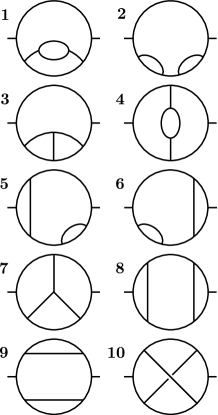
Figure 6: The ten topologies of Feynman diagrams that contribute order $\alpha_{s}^{2}$ terms to $e^{+}e^{-}\to{\it hadrons}$. The incoming and outgoing lines are electroweak vector bosons. The other lines can represent either quarks or gluons. Then a particular contribution to the cross section is given by a particular cut of the diagram, as in Fig. 1.

In this section, we look at some numerical results. As our example, we will consider one of the standard event shape variables, the thrust $t$. We examine the thrust distribution normalized to the total cross section $\sigma\approx(1+\alpha_{s}/\pi)\times\sigma_{0}$ for $e^{+}+e^{-}\to{\it hadrons}$,

$${\cal I}(t)={1\over\sigma}\,{d\sigma\over dt}.$$ (146)

For $t<1$, $d\sigma/dt$ has a contribution, $d\sigma^{(1)}/dt$, of order $\alpha_{s}^{1}$ and a contribution, $d\sigma^{(2)}/dt$, of order $\alpha_{s}^{2}$. Both contributions are included in the next-to-leading order results for ${\cal I}(t)$. We also isolate the second order term, $d\sigma^{(2)}/dt$ and study the second order contributions to the moments of the thrust distribution,

$${I}_{n}={1\over\sigma_{0}(\alpha_{s}/\pi)^{2}}\int_{0}^{1}\!dt\ (1-t)^{n}\ {d\sigma^{(2)}\over dt}.$$ (147)

The first question is whether the gauge choice makes any difference. There are ten topologies of Feynman diagrams that contribute order $\alpha_{s}^{2}$ terms to $e^{+}e^{-}\to{\it hadrons}$. These are shown in Fig. 6. For each topology, we calculate the corresponding contribution to the second moment of the thrust distribution, $I_{2}$. The results are shown in Table 2. We see that graph by graph, the results are completely different in Feynman and Coulomb gauges. However, the total $I_{2}$ summed over graphs is independent of the gauge.

Table 2: Comparison of results in Feynman gauge and Coulomb gauge for $I_{2}$, the second moment of the thrust distribution, Eq. (147). The results are shown for each of the ten graph topologies in Fig. 6. The errors are not shown, but are about 1%. The renormalization scale $\mu$ is chosen to be $\mu=\sqrt{s}$.

graph	Feynman gauge	Coulomb gauge
1	$0.1125$	$-0.3274$
2	$-0.03154$	$-0.01422$
3	$0.2083$	$1.031$
4	$0.1230$	$-0.1955$
5	$-0.1602$	$-0.1834$
6	$-0.1597$	$-0.1828$
7	$1.820$	$1.584$
8	$-0.2222$	$-0.1409$
9	$-0.01243$	$0.03432$
10	$-0.1227$	$-0.04512$
TOTAL	$1.555$	$1.560$

Next, we test whether the Coulomb gauge calculation is working properly by checking whether $I_{n}$ calculated in Coulomb gauge matches $I_{n}$ calculated in Feynman gauge for several choices of $n$. (The results for Feynman gauge were checked against the program of Kunszt and Nason KN in Ref. beowulfPRD .) The results are presented in Table 3. We see that the results are properly gauge invariant within the errors of the program.

Table 3: Comparison of results in Feynman gauge and Coulomb gauge for moments $I_{n}$ of the thrust distribution, Eq. (147). The first error is statistical, the second systematic (determined from the sensitivity to certain cutoffs used to control roundoff errors). We choose $\mu=\sqrt{s}$.

n	Feynman gauge	Coulomb gauge
1.5	$\ 4.127\pm 0.008\pm 0.025$	$\ 4.118\pm 0.010\pm 0.020$
2.0	$\ 1.565\pm 0.002\pm 0.007$	$\ 1.561\pm 0.003\pm 0.006$
2.5	$(6.439\pm 0.010\pm 0.022)\times 10^{-1}$	$(6.423\pm 0.013\pm 0.021)\times 10^{-1}$
3.0	$(2.822\pm 0.005\pm 0.009)\times 10^{-1}$	$(2.816\pm 0.006\pm 0.009)\times 10^{-1}$
3.5	$(1.296\pm 0.002\pm 0.004)\times 10^{-1}$	$(1.294\pm 0.003\pm 0.004)\times 10^{-1}$
4.0	$(6.159\pm 0.011\pm 0.016)\times 10^{-2}$	$(6.156\pm 0.015\pm 0.018)\times 10^{-2}$
4.5	$(3.009\pm 0.006\pm 0.007)\times 10^{-2}$	$(3.010\pm 0.008\pm 0.009)\times 10^{-2}$
5.0	$(1.501\pm 0.003\pm 0.003)\times 10^{-2}$	$(1.503\pm 0.004\pm 0.004)\times 10^{-2}$

Having seen that the program appears to be working properly, we exhibit a graph of the next-to-leading order thrust distribution ${\cal I}(t)$ versus t in Fig. 7. We also show the same distribution calculated at leading order and data from the Opal Collaboration thedata . The theoretical results are rather sensitive to the choice of the $\overline{\rm MS}$ renormalization scale $\mu$. We have chosen $\mu$ to be half of a typical jet energy in a three jet event, $\sqrt{s}/3$. That is, $\mu=\sqrt{s}/6$. The agreement between theory and data is not perfect, but this is to be expected in a strictly perturbative expansion that includes only the first two terms and no correction for effects beyond perturbation theory such as hadronization effects.

As mentioned in the introduction, one may wish to go beyond pure next-to-leading order calculations by incorporating, in an approximate way, some effects at all orders in $\alpha_{s}$. For instance, one may want to include renormalon effects by letting $\alpha_{s}$ run as a function of loop momenta inside graphs. Alternatively, one may also want to simulate realistic final states by adding parton showers to the next-to-leading order calculation. For such applications, one must approximate, and the presence of unphysical degrees of freedom propagating over long distances makes approximation difficult. A straightforward remedy is to do the calculation in a physical gauge, such as Coulomb gauge. In this paper we have seen how this goal can be accomplished.

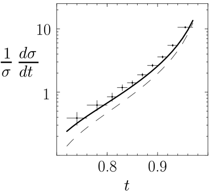
Figure 7: The thrust distribution at $\sqrt{S}=M_{Z}$ calculated in Coulomb gauge at next-to-leading order. We also show, with a dashed curve, the same distribution calculated at leading order. In both cases, the renormalization scale is chosen to be $\mu=\sqrt{S}/6$. We take $\alpha_{s}(M_{Z})=1.118$. The difference between the two theory curves can be taken as an indication of the theory error arising from neglect of graphs beyond order $\alpha_{s}^{2}$. The theory curves are compared to data from the Opal Collaboration thedata .

Appendix A Results for Feynman gauge

It is useful to have at hand the formulas for Feynman gauge that are analogous to what we have found in Coulomb gauge. We present the needed formulas in this appendix.

For the gluon propagator with a self-energy insertion, there is a problem that we treat as described in beowulfPRL ; beowulfPRD . The problem is most easily seen with the virtual self-energy graph. We know that $\Pi^{\alpha\beta}\propto(q^{2}g^{\alpha\beta}-q^{\alpha}q^{\beta})$. The first term is fine since it contains a factor $q^{2}$ that cancels the $1/q^{2}$ in the adjoining propagator. The next term does not have this good property, but its contribution will cancel in a sum over graphs because it is proportional to $q^{\alpha}$ and $q^{\beta}$. In order to make this cancellation happen in a single graph, we replace

$$(-g^{\mu}_{\alpha})(-g^{\nu}_{\beta})\Pi^{\alpha\beta}$$ (148)

by

$$(-g^{\mu}_{\alpha}+q^{\mu}\tilde{q}_{\alpha}/\tilde{q}^{2})(-g^{\nu}_{\beta}+q^{\nu}\tilde{q}_{\beta}/\tilde{q}^{2})\Pi^{\alpha\beta}.$$ (149)

This does not change the answer after summing over graphs because the added terms are proportional to $q^{\mu}$ or $q^{\nu}$. But now the $q^{\alpha}q^{\beta}$ term in $\Pi^{\alpha\beta}$ gives zero in each graph because $(-g^{\mu}_{\alpha}+q^{\mu}\tilde{q}_{\alpha}/\tilde{q}^{2})q^{\alpha}=0$. We make this replacement for both the virtual and real versions of $\Pi^{\alpha\beta}$.

For the real gluon self-energy graph, Eq. (40) becomes

$$N_{TT} = 2C_{A}\bigl{\{}-1+x(1-x)\bigr{\}}+N_{F}\bigl{\{}1-2x(1-x)\bigr{\}},$$

$$N_{tt} = 4C_{A}\,x(1-x)-4N_{F}\,x(1-x),$$

$$N_{EE} = -C_{A}\bigl{\{}1+4x(1-x)\bigr{\}}+4N_{F}\,x(1-x),$$

$$N_{Et} = -2C_{A}(2x-1)+2N_{F}(2x-1).$$ (150)

For the virtual gluon self-energy graph, Eq. (53) becomes

$$A^{\prime\prime}_{T,0} = C_{A}{1\over q^{2}}\biggl{\{}{1\over 2}\,\bar{q}^{2}-{5\over 2}\,q^{2}+2\bar{q}^{2}\,x(1-x)\biggr{\}}+N_{F}{1\over q^{2}}\biggl{\{}\bar{q}^{2}-{x(1-x)\over(1-\epsilon)}\ 2\bar{q}^{2}\biggr{\}},$$

$$A^{\prime\prime}_{T,1} = 0,$$

$$A^{\prime\prime}_{T,2} = 0.$$ (151)

After subtracting $q^{2}A_{T}(q^{2})$ at $q^{2}=0$ from $q^{2}A_{T}(q^{2})$, we are left with the revised version of Eq. (54),

$$A^{\prime}_{T,0} = 2\,C_{A}\bigl{\{}-1+x(1-x)\bigr{\}}+N_{F}\biggl{\{}1-{2x(1-x)\over(1-\epsilon)}\biggr{\}},$$

$$A^{\prime}_{T,1} = 0,$$

$$A^{\prime}_{T,2} = 0.$$ (152)

After renormalization, we have the revised version of Eq. (60),

$$A_{T,0} = -(2C_{A}-N_{F})\,{q^{2}+e^{2}\mu^{2}\over\bar{q}^{2}+e^{2}\mu^{2}}\,+2C_{A}\,x(1-x)\,{q^{2}+e^{5/3}\mu^{2}\over\bar{q}^{2}+e^{5/3}\mu^{2}}$$

$$-2N_{F}\,x(1-x)\,{q^{2}+e^{8/3}\mu^{2}\over\bar{q}^{2}+e^{8/3}\mu^{2}},$$

$$A_{T,1} = 0,$$

$$A_{T,2} = 0.$$ (153)

In Feynman gauge, the second term in the decomposition Eq. (71) is not there, so that

$$F_{g}^{\mu\nu}(q)=D(q)^{\mu\nu}A_{T}(q^{2}).$$ (154)

That is, $A_{E}(q^{2})=A_{T}(q^{2})$ in Eq. (71).

For the quark propagator with a self-energy insertion, we simply change the gauge in the previous Coulomb gauge calculation. Then the coefficients for a quark propagator with a cut self-energy diagram are given by a revised form of Eq. (88),

$$N_{L} = C_{F}\bigl{\{}4x(1-x)+(2x-1)(2x+\Delta)\bigr{\}},$$

$$N_{E} = 2C_{F}\,{(1-x)},$$

$$N_{t} = 2C_{F}.$$ (155)

For the virtual quark self-energy, we begin with the revised form of Eq. (96),

$$B^{\prime\prime}_{L,0} = C_{F}(1-\epsilon),$$

$$B^{\prime\prime}_{L,1} = 0,$$

$$B^{\prime\prime}_{L,2} = 0.$$ (156)

Then $B_{L,J}^{\prime}=B_{L,J}^{\prime\prime}$. After renormalization, we have the revised form of Eq. (99),

$$B_{L,0} = C_{F}\,{q^{2}+e^{1}\mu^{2}\over\bar{q}^{2}+e^{1}\mu^{2}}\ ,$$

$$B_{L,1} = 0,$$

$$B_{L,2} = 0.$$ (157)

In Feynman gauge, the second term in the decomposition (93) is not there, so that

$$F_{q}(q)=\hbox to0.0pt{/\hss}q\,B_{L}(q^{2}).$$ (158)

That is, $B_{E}(q^{2})=0$ in Eq. (93).

The coefficients needed in the renormalization of the quark-antiquark-vector boson three point functions change when we go from Coulomb gauge to Feynman gauge. Specifically, in place of Eq. (135) we have

$$C=C_{A}/2,$$

$$A_{1}(\epsilon)=-2,\ \ \ \ \ A_{2}(\epsilon)=0,\ \ \ A_{3}(\epsilon)=-4(1-\epsilon),$$

$$A_{4}(\epsilon)=0,\ \ \ \ \ \ \ A_{5}(\epsilon)=0,\ \ \ A_{6}(\epsilon)=0,$$

$$B_{1}(\epsilon)=2,\ \ \ \ \ \ \ B_{2}(\epsilon)=0.$$ (159)

In place of Eq. (136) we have

$$C=C_{F}-C_{A}/2=-1/(2N_{C}),$$

$$A_{1}(\epsilon)=-2(1-\epsilon),\ \ A_{2}(\epsilon)=0,\ \ A_{3}(\epsilon)=4(1-\epsilon),$$

$$A_{4}(\epsilon)=0,\ \ \ \ \ \ \ \ \ \ \ \ \ A_{5}(\epsilon)=0,\ \ A_{6}(\epsilon)=0,$$

$$B_{1}(\epsilon)=2,\ \ \ \ \ \ \ \ \ \ \ \ \ B_{2}(\epsilon)=0.$$ (160)

References

• (1) D. E. Soper, Phys. Rev. Lett. 81, 2638 (1998) [hep-ph/9804454].
• (2) D. E. Soper, Phys. Rev. D 62, 014009 (2000) [hep-ph/9910292].
• (3) D. E. Soper, Phys. Rev. D 64, 034018 (2001), [hep-ph/0103262].
• (4) D. E. Soper, Beowulf 1.1 Technical Notes, http://zebu.uoregon.edu/$\sim$soper/beowulf/.
• (5) D. E. Soper, beowulf Version 2.0, http://zebu.uoregon.edu/$\sim$soper/beowulf/.
• (6) Z. Kunszt and D. E. Soper, Phys. Rev. D 46, 192 (1992).
• (7) R. K. Ellis, D. A. Ross and A. E. Terrano, Nucl. Phys. B 178, 421 (1981).
• (8) Z. Kunszt, P. Nason, G.  Marchesini and B. R. Webber in Z Physics at LEP1, Vol. 1, edited by B. Altarelli, R. Kleiss ad C. Verzegnassi (CERN, Geneva, 1989), p. 373
• (9) N.H. Christ and T. D. Lee, Phys. Rev. D 22, 939 (1980).
• (10) G. Leibbrandt and J. Williams, Nucl. Phys. B475, 469 (1996) and subsequent papers.
• (11) M. Z. Akrawy et al. [OPAL Collaboration], Z. Phys. C 47, 505 (1990).