Do solar neutrinos decay?

Abstract

Despite the fact that the solar neutrino flux is now well-understood in the context of matter-affected neutrino mixing, we find that it is not yet possible to set a strong and model-independent bound on solar neutrino decays. If neutrinos decay into truly invisible particles, the Earth-Sun baseline defines a lifetime limit of $\tau/m\gtrsim 10^{-4}$ s/eV. However, there are many possibilities which must be excluded before such a bound can be established. There is an obvious degeneracy between the neutrino lifetime and the mixing parameters. More generally, one must also allow the possibility of active daughter neutrinos and/or antineutrinos, which may partially conceal the characteristic features of decay. Many of the most exotic possibilities that presently complicate the extraction of a decay bound will be removed if the KamLAND reactor antineutrino experiment confirms the large-mixing angle solution to the solar neutrino problem and measures the mixing parameters precisely. Better experimental and theoretical constraints on the ⁸B neutrino flux will also play a key role, as will tighter bounds on absolute neutrino masses. Though the lifetime limit set by the solar flux is weak, it is still the strongest direct limit on non-radiative neutrino decay. Even so, there is no guarantee (by about eight orders of magnitude) that neutrinos from astrophysical sources such as a Galactic supernova or distant Active Galactic Nuclei will not decay.

I Introduction

Since solar neutrinos have been detected with roughly the expected flux, it appears that they do not decay over the 500 s $\times\ c$ distance to Earth. Furthermore, neutrinos from SN1987a were also detected in reasonable numbers on a much longer baseline of ($5\times 10^{12}$ s) $\times\ c$. Decay will deplete the flux of neutrinos of energy $E$ and mass $m$ over a distance $L$ by the factor

$$\exp\left(-\frac{t}{\tau_{lab}}\right)=\exp\left(-\frac{L}{E}\times\frac{m}{\tau}\right)\,,$$ (1)

where $\tau$ is the rest-frame lifetime and we use $c=1$ units from now on. In Table I, we list representative $\tau/m$ scales for various neutrino sources.

Table 1: Representative scales for neutrino lifetimes, taken simply as $\tau/m\sim L/E$. The top three entries correspond to present data, and the lower two to possible future data (after neutrinos of all flavors have been observed from a Galactic supernova and neutrinos from astrophysical sources like active galactic nuclei (AGN) have been observed in km³ detectors).

Neutrino source	$L/E$	$\tau/m$ (s/eV)
Accelerator	30 m/10 MeV	$10^{-14}$
Atmosphere	$10^{4}$ km/300 MeV	$10^{-10}$
Sun	500 s/5 MeV	$10^{-4}$
Supernova	10 kpc/10 MeV	$10^{5}$
AGN	100 Mpc/1 TeV	$10^{4}$

In this paper, we critically assess what the best limits on neutrino decay are. We find that it is not yet possible to set model-independent bounds, even for the well-measured solar neutrinos. We discuss how decay limits can be improved in the future.

Though in the past neutrino decay was frequently discussed in terms of flavor eigenstates, the lifetimes of neutrinos are only well-defined for mass eigenstates (a flavor state does not have a definite mass, lifetime, or magnetic moment). Since we now know that mixing angles are large, this distinction is essential.

Therefore, in considering the decay of neutrinos from the Sun and SN1987a, one has to properly assess the mass eigenstate content of the fluxes. The SN1987a data can be reasonably explained by saying that the expected flux of $\bar{\nu}_{1}$ made it to Earth and was detected as $\bar{\nu}_{e}$ via the charged-current reaction $\bar{\nu}_{e}p\rightarrow e^{+}n$. The $\bar{\nu}_{\mu}$ component would only have been detectable in neutral-current reactions, and the SN1987a data are consistent with no neutral-current events. If $\nu_{1}$ is (as suggestively labeled) the lightest mass eigenstate, then it would not be kinematically allowed to decay, so that the decay limit from SN1987a would be meaningless.

Presently, the best explanation of the solar neutrino problem is large mixing angle (LMA) Mikheyev-Smirnov-Wolfenstein (MSW) transformation of $\nu_{e}$ to $\nu_{\mu},\nu_{\tau}$. Besides being the best oscillation-parameter fit, LMA also provides a “good” fit to all of the solar neutrino data in terms of an acceptable chi-squared. Without the effects of oscillations, the solar neutrino flux is only understood at the factor of two level. Including the effects of oscillations, the total flux of all flavors is better understood, and the hope is that much more stringent decay limits can be derived. A similar approach was used to set the strongest direct neutrino magnetic moment limit magnetic .

If LMA is the correct scenario, then solar neutrinos in the $5-15$ MeV energy range are created as nearly pure $\nu_{2}$ mass eigenstates. Furthermore, their propagation in the Sun is completely adiabatic, so that they emerge as pure $\nu_{2}$ eigenstates, where $m_{2}>m_{1}$. Since the characteristic signature of decay is its energy dependence, we restrict our attention to this energy range, over which Super-Kamiokande (SK) SK and the Sudbury Neutrino Observatory (SNO) SNO have measured energy spectra. This data may thus be used to search for the signatures of the kinematically allowed $\nu_{2}\rightarrow\nu_{1}+X$ decay (the decay modes are discussed in detail below).

While neutrino decay was an early proposed explanation of the solar neutrino problem solardecay ; solardecay1 , in this paper we will take the point of view that the LMA solution specifies the correct basic picture and will consider $\nu_{2}\rightarrow\nu_{1}+X$ decay as a perturbation, with the goal of placing a limit on $\tau/m$ (since $m$ is unknown, only the quantity $\tau/m$ can be constrained). Ongoing experiments will soon confirm or refute the LMA solution.

While there are strong limits on radiative neutrino decays RPP ; raffelt , in this paper we consider only the so-called “invisible” decays, i.e., decays into possibly detectable neutrinos (or antineutrinos) plus truly invisible particles, e.g., light scalar or pseudoscalar bosons. For these modes, the lifetime limits are very weak indeed; see Table I. There are also limits from cosmology, the strongest of which use the cosmic microwave background data cosmolimits . The effect searched for arises because of the transfer of nonrelativistic energy density in the parent neutrinos ($m\gtrsim 10$ eV) to relativistic energy density in the daughter neutrinos ($m\simeq 0$). Neither the large mass of the parent neutrino nor the huge mass splitting is supported by present data, so these cosmological limits on non-radiative neutrino decays are inapplicable.

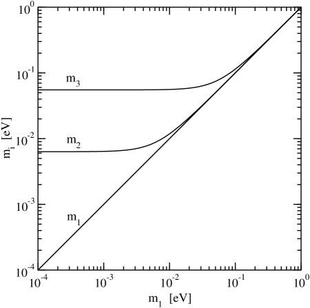
Figure 1: The values of the neutrino mass eigenvalues as a function of the unknown smallest mass $m_{1}$. When $m_{1}$ is specified, the measured solar and atmospheric $\delta m^{2}$ values fix $m_{2}$ and $m_{3}$. For an inverted hierarchy ($\delta m^{2}_{atm}<0$), the two upper eigenvalues are very nearly degenerate at the position of the curve labeled $m_{3}$. The present bound on neutrino mass from tritium experiments is about 2 eV tritium ; by the construction above, it applies to all three mass eigenvalues.

While detection of daughter neutrinos or antineutrinos has been considered in the literature, it has nearly always been with the assumption that $m_{1}\ll m_{2}$, and that the daughter neutrino carries half the energy of its parent in a two-body decay. These assumptions are not generally valid. Since oscillation experiments do not determine the overall mass scale, the lightest mass eigenvalue $m_{1}$ is unknown. However, for fixed $m_{1}$, the masses $m_{2}$ and $m_{3}$ are determined by the measured mass-squared differences. Thus

$$m_{2}=\sqrt{m_{2}^{2}-m_{1}^{2}+m_{1}^{2}}=\sqrt{m_{1}^{2}+\delta m^{2}_{sol}}\,,$$ (2)

where solar-neutrino data give $\delta m^{2}_{sol}\simeq 4\times 10^{-5}$ eV², and similarly,

$$m_{3}=\sqrt{m_{1}^{2}+\delta m^{2}_{sol}+\delta m^{2}_{atm}}\,,$$ (3)

where atmospheric-neutrino data give $\delta m^{2}_{atm}\simeq 3\times 10^{-3}$ eV². All three masses are shown in Fig. 1, illustrating that the masses are nearly degenerate unless the overall mass scale is tiny. The accepted wisdom is that neutrino masses should be strongly hierarchical, e.g., in see-saw models, proportional to the squares of charged-lepton masses. Note that the ratio $m_{3}/m_{2}\lesssim 10$ for all $m_{1}$. Naively, this argues against a simple see-saw mass pattern and argues for the idea that the mass ratios can be small, and quite possibly degenerate.

If the neutrino masses are degenerate, then the daughter neutrino carries nearly the full energy of the parent neutrino in any reference frame (in the rest frame, a $\nu_{2}$ at rest decays to a $\nu_{1}$ nearly at rest). This completely alters scenarios in which active daughters are detected.

II Neutrino Decay Models

Non-radiative neutrino decay may arise through the coupling of the neutrino to a very light or massless particle, such as a Majoron majoronmodels . Majoron models typically have tree-level scalar or pseudoscalar couplings of the form

$${\cal L}=g_{ij}\overline{\nu}_{i}\nu_{j}\chi+h_{ij}\overline{\nu}_{i}\gamma_{5}\nu_{j}\chi+{\rm h.c.},$$ (4)

where $\chi$ is a massless Majoron, which does not carry definite lepton number. For the couplings specified by Eq. (4), the decay rates into neutrino and antineutrino daughters are given by Ref. kim

$$\Gamma_{\nu_{2}\rightarrow\nu_{1}} = \frac{m_{1}m_{2}}{16\pi E_{2}}\left[g^{2}\left(\frac{x}{2}+2+\frac{2}{x}\ln x-\frac{2}{x^{2}}-\frac{1}{2x^{3}}\right)\right.\,$$ (5)

$$+ \left.h^{2}\left(\frac{x}{2}-2+\frac{2}{x}\ln x+\frac{2}{x^{2}}-\frac{1}{2x^{3}}\right)\right],$$

$$\Gamma_{\nu_{2}\rightarrow\overline{\nu}_{1}} = \frac{m_{1}m_{2}}{16\pi E_{2}}\left(g^{2}+h^{2}\right)\left[\frac{x}{2}-\frac{2}{x}\ln x-\frac{1}{2x^{3}}\right]\,,$$ (6)

where $x=m_{2}/m_{1}$, and we have dropped the subscripts on the coupling constants. The decay widths in this section are defined in the laboratory frame, so the relation to the rest-frame lifetimes quoted elsewhere is

$$\frac{\tau}{m}=\frac{1}{m\,\Gamma_{rest}}=\frac{1}{E\,\Gamma_{lab}}\,.$$ (7)

In the limit of hierarchical neutrino masses, $m_{2}\gg m_{1}$, the case that has received the most attention to date, the decay rates are equal:

$$\Gamma_{\nu_{2}\rightarrow\nu_{1}}=\Gamma_{\nu_{2}\rightarrow\overline{\nu}_{1}}=\frac{(g^{2}+h^{2})}{32\pi}\,\frac{m_{2}^{2}}{E_{2}}\,.$$ (8)

In the opposite limit, where $m_{2}\rightarrow m_{1}$ (but keeping $\delta m^{2}\neq 0$), we find instead:

$$\Gamma_{\nu_{2}\rightarrow\nu_{1}} = \frac{g^{2}}{16\pi}\,\frac{\delta m^{2}}{4E_{2}}\;+\;h^{2}\times{\cal O}\left(\frac{\delta m^{2}}{m_{2}^{2}}\right)^{3}\,,$$

$$\Gamma_{\nu_{2}\rightarrow\overline{\nu}_{1}} = \frac{(g^{2}+h^{2})}{16\pi}\,\frac{m_{2}^{2}}{E_{2}}\times{\cal O}\left(\frac{\delta m^{2}}{m_{2}^{2}}\right)^{3}\,.$$ (9)

The important point to note is that in these Majoron models, both neutrino and antineutrino decay products may be produced, but the relative weight of the two decay modes depends strongly upon the mass hierarchy.

In the simplest versions of these models, the neutrino masses are proportional to these coupling constants and hence the neutrinos are exactly stable, as the matrix of coupling constants is diagonal in the mass basis. Even in this case, the neutrinos may have finite lifetimes in matter, as the rotation of the mass basis in matter will lead to non-diagonal couplings between matter mass eigenstates valle ; matterdecay . In the most general case, the basic models can easily be modified to permit non-diagonal couplings in vacuum fastdecay .

While there are a huge variety of Majoron models in the literature including, for instance, “charged” Majoron burgess and “vector Majoron” carone models, we will not restrict our attention to any particular model. For example, instead of a Majoron model per se, we can consider the couplings of neutrinos to a very light gauge boson. Similarly, we make no assumption about the relationship between the neutrino masses and the couplings that give rise to decay, or whether the neutrinos are Dirac or Majorana particles.

We thus take a purely phenomenological point of view and consider any possible tree-level coupling between the neutrinos and a very light or massless particle. We shall consider the cases where the decay products are active or sterile neutrinos or antineutrinos, plus an “invisible” particle. While one could imagine models where such a coupling is absent at tree level (as with radiative decay in the Standard Model, for example), models of this sort are of less interest, as any coupling arising only at loop level is likely to lead to a very small decay rate.

Bounds on neutrino-Majoron couplings of the form in Eq. (4) may be obtained from considering their effects on the two-body leptonic decays of $\pi$ and $K$ mesons at rest. A nonzero coupling allows the final neutrino to also appear as a neutrino or antineutrino, plus a Majoron. This increases the decay rate and also smears the momentum distribution of the charged lepton. The bounds obtained are approximately $g^{2}\lesssim 10^{-4}$ meson ; britton , and are reasonably model-independent. (Note that in this section we denote by $g$ either a scalar or pseudoscalar coupling). A considerably more stringent bound may be derived from limits on neutrinoless double beta decay with Majoron emission zuber . However, the limit of $g^{2}\lesssim 10^{-8}$ applies only to the $g_{ee}$ element of the coupling matrix and does not directly translate into a bound on the parameter of interest, namely $g_{21}$.

Translated into a bound on neutrino lifetimes, the meson-decay bound on the coupling of $g^{2}\lesssim 10^{-4}$ becomes

$$\frac{\tau}{m}\gtrsim 3\times 10^{-5}\ \rm{s/eV}\left(\frac{10^{-5}\ \rm{eV}^{2}}{\delta m^{2}}\right)\,,$$ (10)

where we have used Eq. (8). With the solar $\delta m^{2}\simeq 4\times 10^{-5}$ eV², the lifetime limit obtained allows substantial decay of solar neutrinos (from Table I, the natural scale of the problem is $\tau/m\simeq 10^{-4}$ s/eV). If the mass hierarchy is inverted, then solar neutrino decays can also occur with $\delta m^{2}\simeq 10^{-3}$ eV², in which case the derived lifetime limit is 100 times weaker, and hence not useful.

We emphasize again that it is not our intention to restrict our attention only to the case of Majoron models. We discuss these models only as a concrete example of the types of decay modes that may be expected. In Section III we take a quite general perspective and discuss specific decay modes as illustrative, model-independent examples.

III Solar $\nu_{2}$ Decay

We consider the decay of neutrinos during their journey from the Sun to Earth, and neglect decay inside the Sun, since the distances are 500 s and 2 s, respectively. Decay rates can be increased in matter matterdecay by the greater phase space provided by the matter enhancement to $\delta m^{2}$. However, for LMA-type solutions, this effect is not large. If decay in the Sun were significant it would imply that our understanding of the solar neutrino flux is fundamentally flawed; KamLAND and future solar-neutrino experiments will check this possibility.

As noted, since an identifying characteristic of decay is its particular energy dependence, we consider only the SK and SNO spectral data. These experiments are sensitive to $5-15$ MeV neutrinos from ⁸B beta decay (while the normalization uncertainty is $\simeq 20\%$, it is common to SK and SNO). While one might think that the lowest energy neutrinos are the best suited for testing decay effects, there are two important caveats. First, the gallium and chlorine radiochemical experiments only measure energy-integrated rates, and receive contributions from several different neutrino sources with uncertain relative normalizations. Exotic effects on the neutrino survival probability can be hidden in this data. Second, for the LMA solutions, the $\nu_{1}$ to $\nu_{2}$ ratio rises at low energies, and as noted, only the heavier $\nu_{2}$ can decay.

In the energy range covered by the SK and SNO spectra, the solar neutrino flux is dominated by the ⁸B neutrinos. To a very good approximation, these neutrinos are produced at the solar center where the matter potential is

$$\zeta\equiv{\sqrt{2}}G_{F}N_{e}\frac{2E}{\delta m^{2}}=15.3\left(\frac{E}{10\ {\rm MeV}}\right)\left(\frac{10^{-5}{\ \rm eV^{2}}}{\delta m^{2}}\right).$$ (11)

The initial $\nu_{1}$ and $\nu_{2}$ fractions of the flux are specified by

$$P_{\nu_{1}}^{i} = \cos^{2}\theta_{m},$$

$$P_{\nu_{2}}^{i} = \sin^{2}\theta_{m},$$ (12)

where the matter mixing angle given by

$$\sin^{2}{2\theta_{m}}=\frac{\sin^{2}{2\theta_{v}}}{\sin^{2}{2\theta_{v}}+(\cos{2\theta_{m}}-\zeta)^{2}}\,,$$ (13)

and $\theta_{v}$ is the vacuum angle. As representative values in the LMA allowed region lma , we choose $\delta m^{2}=4\times 10^{-5}$ eV² and $\sin^{2}{2\theta_{v}}=0.9$. The MSW transformation is always adiabatic in the solar neutrino energy range for the LMA solutions, so the fluxes of $\nu_{1}$ and $\nu_{2}$ are unchanged at the solar surface (neglecting the tiny decay probability over the solar radius). The final $\nu_{1}$ and $\nu_{2}$ fluxes at Earth, taking decay into account are

$$P_{\nu_{1}}^{f} = P_{\nu_{1}}^{i}\,,$$

$$P_{\nu_{2}}^{f} = P_{\nu_{2}}^{i}\exp\left(-\frac{L}{E}\times\frac{m}{\tau}\right)\,.$$ (14)

Note that the small variation in the Earth-Sun distance cannot be exploited, as its effects are washed out by the energy resolution. It is convenient to think of a typical energy for decay (that makes the argument of the exponential unity); in convenient units, this is

$$\frac{E_{decay}}{1{\rm\ MeV}}=\frac{5\times 10^{-4}{\rm\ s/eV}}{\tau/m}\,.$$ (15)

The electron neutrino survival probability at Earth is thus

$$P(\nu_{e}\rightarrow\nu_{e})=P_{\nu_{1}}^{f}\cos^{2}\theta_{v}+P_{\nu_{2}}^{f}\sin^{2}\theta_{v}\,.$$ (16)

The muon neutrino appearance probability is

$$P(\nu_{e}\rightarrow\nu_{\mu})=P_{\nu_{1}}^{f}\sin^{2}\theta_{v}+P_{\nu_{2}}^{f}\cos^{2}\theta_{v}\,.$$ (17)

Because of decay, $P(\nu_{e}\rightarrow\nu_{e})+P(\nu_{e}\rightarrow\nu_{\mu})<1$ (at this point, we are considering all decay products to be sterile).

In the absence of decay or oscillations, the recoil electron spectrum from neutrino-electron scattering in SK can be computed by convolving the ⁸B neutrino spectrum ortiz with the $\nu_{e}-e$ elastic scattering cross section $d\sigma/dT$ (see, e.g., Ref magnetic ), and smearing with the SK energy resolution SKres . For a given decay or oscillation scenario, the spectrum is calculated in the same way, but now allowing an energy-dependent survival probability for the neutrinos. The contribution (about 6 times smaller, and with a slightly different differential cross section) from $\nu_{\mu}-e$ elastic scattering must also be included. These two spectra, binned every 0.5 MeV in the recoil electron total energy $E_{e}=T_{e}+m_{e}$ can then be divided bin-by-bin. The resulting “ratio spectrum” $R_{SK}$ closely approximates how SK presents their data, though they of course use a much more detailed Monte Carlo to model the detector response. Also, in their case the numerator in the ratio is the measured counts per bin.

III.1 Simple $\nu_{2}$ Disappearance

In the upper panel of Fig. 2 we display the $\nu_{e}$ survival probability as a function of neutrino energy, for a range of decay rates. We have chosen parameters in the LMA allowed region. The solid curve corresponds to the case of no decay. In the lower panel, we show the corresponding SK electron energy spectrum, which also includes the $\nu_{\mu}$ component. At large energies, the height of the solid lines is set just by $\sin^{2}{2\theta}=0.9$; SNO expects 0.34 and SK expects $0.34+0.66/6=0.45$. The upturn at low energies is set by $\delta m^{2}=4\times 10^{-5}$ eV². Note that the chlorine experiment is mostly sensitive to the ⁸B neutrinos, so also expects $\simeq 1/3$. In order to correctly calculate the rate in the gallium detectors, one must also integrate over the finite source region in the Sun. One can see from the figure that as the neutrino lifetime approaches $10^{-4}{\rm\ s/eV}$ or shorter the spectral shape begins to display a significant deviation from the flat SK ratio spectrum. The total flux also begins to depart significantly from the measured value, though only at about the $2\sigma$ level, taking into account the ⁸B flux uncertainty.

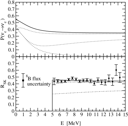
Figure 2: In the upper panel, the electron neutrino survival probability is shown versus neutrino energy. In the lower panel, the ratio of measured to expected spectra in SK is shown versus the recoil electron total energy, as detected in neutrino-electron scattering above 5 MeV. The solid lines correspond to the LMA solution ($\delta m^{2}=4\times 10^{-5}$ eV², $\sin^{2}{2\theta}=0.9$) with stable $\nu_{2}$. The dashed lines, in order of decreasing height, correspond to $\nu_{2}$ lifetimes of $\tau/m=10^{-3},10^{-4},{\rm and\ }10^{-5}$ s/eV (by Eq. (15), these correspond to decays at typical energies of 0.5, 5, and 50 MeV, respectively). The 1258-day data from SK are shown in the lower panel, as is the size of the flux normalization uncertainty. The decay products of $\nu_{2}$ are considered to be sterile.

III.2 Compensating Effects from Oscillations

In Fig. 2 we used the flatness of the SK spectrum to estimate a bound on the decay rate of $\nu_{2}$. However, things may not be as straightforward as this basic case. In particular, since oscillation effects may lead to an energy distortion, we must address the possibility that a cancellation between oscillation and decay survival probabilities may produce an acceptably flat spectrum.

For example, we could choose a $\delta m^{2}$ somewhat larger than those in the allowed LMA region, so that the $\nu_{e}$ survival probability begins to rise toward the lower energy end of the SK energy range. Since the decay rate is larger for lower energy neutrinos, the question then becomes whether the decay might be “just so” in the sense that it conspires to cancel this tilt in the survival probability, resulting in a spectrum which is apparently flat. Such a scenario has recently been addressed in Ref. choubey ; chou ; joshipura . We view this scenario as somewhat unnatural, however we agree that it cannot be excluded.

In Fig. 3, we show an example of such a conspiracy, using oscillation parameters for which, in the absence of decay, the SK spectrum is not very flat. Here, if we choose a lifetime of order $10^{-4}{\rm\ s/eV}$ we see that a reasonably flat spectrum may be regained. Note however, the large difference between the solid and dashed curves in this figure, both in terms of the spectral shape and the overall rates. It is important to realize that KamLAND will essentially break the degeneracy between the oscillation parameters and the neutrino lifetime, giving a prediction for the mixing effects (without decay) on the solar neutrino spectrum. One can then go and look for a deviation from this prediction in the solar neutrino spectrum. As is clear from Figs. 2 and 3, a lifetime of order $10^{-4}{\rm\ s/eV}$ defines the scale at which decay could possibly be distinguished.

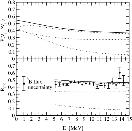
Figure 3: An example of the parameter degeneracy between the lifetime and the mixing parameters is illustrated. The description is as for Fig. 2, except that now $\delta m^{2}=12\times 10^{-5}$ eV², which flattens $R_{SK}$ for $\tau/m=10^{-4}$ s/eV, making it consistent with the SK spectral shape. It is about $1\sigma$ discrepant in terms of normalization.

III.3 Appearance of Active Daughter $\nu_{1}$

Another possible complication is the possible detection of neutrinos produced as decay products. The replacement of a parent neutrino with an active daughter may partially hide the effects of decay. Unlike the situation discussed above, this would not be sensitive to a conspiracy between parameters. Rather, the appearance and possible detection of active decay products is a quite generic expectation, as most plausible decay models will feature a neutrino or antineutrino in the final state. There are a range of model-dependent possibilities for these final-state neutrinos, such as whether the neutrinos are Dirac or Majorana particles and whether the decay products are active or sterile dodelson . In this subsection we study the effects of active daughter neutrinos.

If active daughters are produced, the overall neutrino mass scale is important. In virtually all studies of neutrino decay, it has been assumed that the neutrino mass spectrum is hierarchical, and thus the mass of the final state neutrino may be neglected. This is important, since the energy difference between initial and final state neutrinos depends on the values of the masses. If a neutrino decays to a massless particle and another neutrino, the fraction of the initial neutrino energy carried by the final state neutrino ranges from a maximum of $E_{f}/E_{i}\simeq 1$ to a minimum of $E_{f}/E_{i}\simeq m_{1}^{2}/m_{2}^{2}$. Where a hierarchical mass spectrum is a good approximation, the two decay products will each carry a large fraction of the original neutrino energy, hence the daughter neutrino will, on average, be degraded in energy. However, if the neutrino masses are degenerate, the daughter neutrino must have approximately the same energy as the parent neutrino. For example, if we take $\delta m^{2}\simeq 4\times 10^{-5}\rm{\ eV}^{2}$ and the degenerate mass larger than about $m_{1}\simeq m_{2}\simeq 0.03{\rm\ eV}$ the energy degradation of the daughter neutrino would be less than about 0.5 MeV – the width of the SK energy bins.

Given this, one may wonder if it is possible to set any decay bound at all. For example, if the mixing angle were exactly maximal, any decay of $\nu_{2}$ to $\nu_{1}$ in which the neutrino energy was not degraded would be undetectable. However, the solar $\nu_{e}$ survival probability appears to be less than 1/2 in the SNO/SK and Cl energy region (and somewhat larger in the Ga region) strongly disfavoring exact maximal mixing. As long as the mixing angle is not exactly maximal, decay will cause the relative fluxes of $\nu_{e}$ and $\nu_{\mu}$ to vary as a function of energy, which would be distinguishable in both SK and SNO.

In Fig. 4 we demonstrate the effect on the spectrum if $\nu_{2}$ decays to the orthogonal state $\nu_{1}$, in the limit where the daughter neutrinos carry the full energy of the parent. The expressions in Eq. (III) have now to be replaced by

$$P_{\nu_{1}}^{f} = P_{\nu_{1}}^{i}+P_{\nu_{2}}^{i}\left[1-\exp\left(-\frac{L}{E}\times\frac{m}{\tau}\right)\right],$$

$$P_{\nu_{2}}^{f} = P_{\nu_{2}}^{i}\exp\left(-\frac{L}{E}\times\frac{m}{\tau}\right).$$ (18)

in order to include the $\nu_{1}$ produced by the decay of $\nu_{2}$. Note that there is no quantum-mechanical interference between $\nu_{1}$ originally in the beam with those produced by the decays of $\nu_{2}$ ohlsson . In addition, we may take the daughter neutrinos to be collinear with the parent neutrinos ohlsson .

An interesting feature of Fig. 4 is the direction of the deviation from a flat spectrum. Rather than a deviation downward (as observed in Fig. 2) caused by the depletion of the flux at lower energies, we instead obtain a deviation upward. This is due to the replacement of a portion of the $\nu_{2}$ flux by $\nu_{1}$, which has a larger $\nu_{e}$ component (since $\theta_{solar}\simeq 36^{\circ}$). Note, however, that the size of $\tau/m$ where decay effects show up as a significant deviation (either to the flat spectrum, or to the total rates) is comparable to that shown in Fig. 2. Therefore, the lifetime limits for the cases of decay to steriles and decay to active neutrinos of non-degraded energy could be comparable (if $m_{1}\simeq m_{2}$ were known).

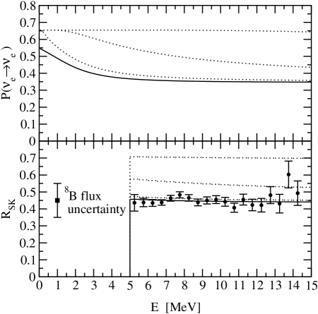
Figure 4: The effect of $\nu_{2}$ decay to active $\nu_{1}$ daughters is shown. We have assumed $m_{1}$ and $m_{2}$ are nearly degenerate, so that the daughter energy is approximately the full energy of the parent. The description is as for Fig. 2, except that now the dotted lines, in order of increasing height, correspond to $\nu_{2}$ lifetimes of $\tau/m=10^{-3},10^{-4},{\rm and\ }10^{-5}$ s/eV. Again, the case $\tau/m=10^{-4}$ s/eV is discrepant in terms of shape and normalization.

III.4 Dark-Side Inversion Undone by Decay

We now consider an unusual case that requires decay. Suppose the solar neutrino parameters live on the so-called “dark-side” dark of the parameter space, that is, the hierarchy is inverted such a way that $\nu_{2}$ has a larger $\nu_{e}$ component than does $\nu_{1}$. This situation does not provide a good fit to the solar neutrino data, as an MSW resonance would not take place in the Sun and it is not possible to obtain a $\nu_{e}$ survival probability less than one half. However, if we add fast decay to this dark-side solution, we can convert the entire flux to $\nu_{1}$, obtaining a solution that is in good agreement with the SK, SNO and Cl data. That is, decay effectively undoes the $\nu_{2}-\nu_{1}$ reversal in $\nu_{e}$. We have plotted such an example in Fig. 5. Note that the curve which most closely resembles the measured SK data is the one which corresponds to the largest decay rate. The only problem with this solution lies with Ga flux measurement of greater than a half – a difficulty which, alone, is probably sufficient to rule out such a solution. So, although such a scenario seems unlikely, it is enough, however, to give one pause for thought.

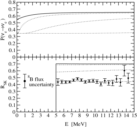
Figure 5: The effect of $\nu_{2}$ decay to active $\nu_{1}$ daughters is shown again, this time with a “dark-side” angle of $54^{\circ}$ instead of $36^{\circ}$ (but still with $\delta m^{2}=4\times 10^{-5}$ eV², $\sin^{2}{2\theta}=0.9$). The description is as for Fig. 2, except that now the dotted lines, in order of decreasing height, correspond to $\nu_{2}$ lifetimes of $\tau/m=10^{-3},10^{-4},{\rm and\ }10^{-5}$ s/eV. In this unusual case, a lifetime as short as $10^{-5}$ s/eV is required to undo the $\nu_{2}/\nu_{1}$ reversal in $\nu_{e}$ caused by choosing a “dark-side” angle.

III.5 Other Possibilities

In Fig. 2 we have considered decay products that are completely undetectable (this could also be achieved if the daughter neutrino energies were artificially taken to zero), while in Fig. 4 we considered active daughters of the full energy, such that their detectability is optimized. It is clear that the case where the daughter neutrino should be active but have degraded energy, lies somewhere between the examples considered in Fig. 2 and Fig. 4. This case would occur if $m_{1}\ll m_{2}$. However, note that this directly modifies the absolute spectrum, which is steeply falling (see Ref SK ); the ratio spectra shown above cannot be averaged by eye. By comparing Figs. 2 and 4, it should be clear that it could be quite difficult to discern such a decay using either the spectral shape or the total flux

Another example is that of the inverted hierarchy, where the solar neutrino flux can decay to the eigenstate that consists mainly of $\nu_{\mu}$ and $\nu_{\tau}$. Since these flavors have a cross-section approximately 6 times smaller than $\nu_{e}$, this situation is closer to the sterile daughters example presented in Fig. 2 than to the active daughter $\nu_{1}$ case presented in Fig. 4.

The decay products might include antineutrinos rather than neutrinos or, more generally, a mixture of the two. Since $\overline{\nu}_{\mu}$ and $\overline{\nu}_{\tau}$ have similar neutrino-electron scattering cross-sections to $\nu_{\mu}$ and $\nu_{\tau}$, they would also be difficult to detect.

In Ref. pakvasadaughters ; choubey , the appearance of $\bar{\nu}_{e}$ as a decay product is discussed. An estimated limit on the solar $\bar{\nu}_{e}$ flux has been obtained for the SK data in Ref. torrente , using the technique of Ref. invbeta , and is quoted as 3.5% of the ⁸B $\nu_{e}$ flux (at the 95% C.L.). Ref. choubey takes this to imply a stringent decay limit of $\tau/m\simeq 10^{-3}$ s/eV. Though they state that the $\bar{\nu}_{1}$ carries less energy than the parent neutrino, it appears that the bound is derived without taking this into account. Indeed, as we have stressed above, the daughter may carry nearly the full energy of the parent. But if not, it makes a big difference for the yield, since the $\bar{\nu}_{e}p\rightarrow e^{+}n$ cross section is nearly quadratic in neutrino energy. And the neutrino spectrum is falling steeply with energy, so decay products from a high energy can be hidden at a lower energy. Also, if the daughter energy is less than the parent energy, then the limit as quoted from Ref. torrente does not apply. The limit of 3.5% assumes that the $\bar{\nu}_{e}$ spectrum has the same shape as the ⁸B $\nu_{e}$ spectrum. If that assumption is relaxed, then the flux limit is more conservatively about 10%. Thus the decay limit is certainly considerably weaker than $\tau/m\simeq 10^{-3}$ s/eV.

Finally, one might reasonably ask if the solar neutrino data can be explained by neutrino decay. The formulation of this question that seems to be the most interesting is this: Can the solar $\nu_{e}$ and LSND lsnd $\bar{\nu}_{e}$ data be made consistent? The combined solar, atmospheric, and LSND results require three independent $\delta m^{2}$ values, whereas only two are allowed in three-generation mixing. Thus, our question can be rephrased: Can one explain all of the data with the two $\delta m^{2}$ values and one $\tau/m$ value? Let us assume the LSND vacuum mixing parameters. For the large $\delta m^{2}\simeq 1$ eV², matter effects in the Sun are negligible. We are free to invert the sign of $\delta m^{2}$ so that the solar $\nu_{e}\simeq\nu_{2}$ (the LSND mixing angle is very small). Suppose decay turns this into $\simeq 1/3\,\nu_{2}+2/3\,\nu_{1}\simeq 1/3\,\nu_{e}+2/3\,\nu_{\mu}$ in the SK energy region, roughly matching the SNO and SK observations (we ignore the spectral distortion). But then decay is complete in the gallium-detector energy range, predicting nearly zero $\nu_{e}$ flux there, in gross disagreement with observations.

IV Other Neutrino Decays

Let us suppose that a model-independent limit on solar neutrino decay can be arrived at, and that it reaches the scale of $\tau/m\lesssim 10^{-4}$ s/eV. Once such a limit has been established, can it be used to set meaningful limits on the possible decay of neutrinos from other sources? In particular, we shall consider the decay of atmospheric neutrinos. It is immediately obvious that if we restrict ourselves to the three active neutrinos, it is difficult to arrange for decay to play a role in the atmospheric neutrino problem. Since two of the three mass eigenstates have large $\nu_{e}$ components, it is hard to see how decay could alter the atmospheric $\nu_{\mu}$ flux, while leaving the $\nu_{e}$ flux unaltered, as the data suggests.

We can make this point more precise. Let us define the neutrino mass eigenstates to be such that $m_{3}>m_{2}>m_{1}$. Considered as a function of mass squared, in a normal hierarchy two states are close together (the solar $\delta m^{2}$), and are well below the third state (by the atmospheric $\delta m^{2}$). The sign of the solar $\delta m^{2}$ is fixed by the observation of matter effects in the Sun (for the opposite sign, there is no MSW resonance). However, the sign of the atmospheric $\delta m^{2}$ that dictates vacuum oscillations is unknown. An inverted hierarchy is obtained when this state is well below the solar doublet on a mass-squared scale. See also Fig. 1, but note that the scale there is mass, not mass squared.

If we have a normal hierarchy, the solar decay limit applies to $\tau_{21}/m_{2}$, whereas if we have an inverted hierarchy, the limit applies to both $\tau_{32}/m_{3}$ and $\tau_{31}/m_{3}$. In the inverted case, only $\nu_{2}\rightarrow\nu_{1}$ is not directly constrained (in the inverted case, we relabel so that $m_{3}>m_{2}>m_{1}$). However, since this decay mode has virtually the same phase space as $\nu_{3}\rightarrow\nu_{1}$, it must also be constrained, unless there were a large hierarchy in the respective couplings. It is important to remember that the flavor content of the mass eigenstates is irrelevant for their decays.

In the case of a normal hierarchy, we can translate the bound on $\nu_{2}$ decay into one on $\nu_{3}$ if we make certain assumptions. Since the quantity limited by experiment is $\tau/m_{2}$ and $\tau/m_{2}\sim(g^{2}\delta m^{2})^{-1}$ (using Eq. (8)), then the overall mass scale is mostly irrelevant (at least for the hierarchical case) for setting a bound on $g$. A solar decay limit of $10^{-4}$ s/eV would translate into a limit on the coupling of

$$g^{2}_{21}\lesssim 3\times 10^{-5}\left(\frac{10^{-5}{\rm\ eV}^{2}}{\delta m^{2}}\right)\,.$$ (19)

For the solar LMA solution, $\delta m^{2}\simeq 4\times 10^{-5}$ eV², one would obtain a limit of $g^{2}_{21}<10^{-5}$, slightly more restrictive than the limit from meson decays of $g^{2}\lesssim 10^{-4}$. However, from Section II we see that the correspondence between neutrino lifetime and the coupling constant depends sensitively on the mass hierarchy.

In order to translate a bound on $\nu_{2}$ into one on $\nu_{3}$, we would have to assume that $g$ is approximately universal among generations. Of course, this is a very model-dependent assumption. The limit on the $\nu_{3}$ lifetime would become

$$\frac{\tau_{31}}{m_{3}}\sim\frac{\tau_{21}}{m_{2}}\times\frac{\delta m^{2}_{21}}{\delta m^{2}_{31}}\gtrsim 10^{-6}{\rm\ s/eV}\,.$$ (20)

The natural scale for setting a limit on neutrino decay with atmospheric neutrinos is $\tau/m\simeq L/E\simeq 10^{4}{\rm\ km}/300{\rm\ MeV}\simeq 10^{-10}$ s/eV. Thus if there were significant decay in the atmospheric neutrinos, a significant hierarchy in the couplings $(g_{31}/g_{21})^{2}\sim 10^{4}$ would be required. The exception to this is to greatly increase the $\delta m^{2}$, as in Ref. barger . This model is now strongly disfavored since it cannot accommodate large-angle mixing with an active neutrino in the solar sector. Finally, as noted, if there is an inverted hierarchy, a limit on solar neutrino decay may apply directly to atmospheric neutrino decay, since the same states may be involved.

A limit on solar neutrino decay would also apply to decays to “phantom” neutrinos. Light sterile neutrinos can be used to add new mass eigenstates anywhere relative to the standard hierarchy. These new mass eigenstates might be inaccessible by flavor mixing (or with very small angles), but might be reached via decays (which connect mass eigenstates directly). If so, the presence of these phantom neutrinos could result in an apparent non-unitarity of the $3\times 3$ mixing matrix. Indeed, such tests could infer their existence even if decay were not seen directly. These phantom neutrinos can also be lower in mass than $\nu_{1}$ in the standard case; however, the very long SN1987a lifetime limit frieman would apply to those states.

V Conclusions

Solar and supernova neutrinos have been observed on Earth suggesting, naively, that they do not decay. However, this conclusion cannot immediately be drawn unless one can rule out certain subtleties. When considering these possibilities we must be careful to distinguish the mass eigenstates (for which the lifetimes are properly defined) and the flavor eigenstates.

1. While the LMA solution is an excellent fit to the solar neutrino data, one cannot completely rule out more exotic scenarios until KamLAND kamland confirms the LMA parameters in an experiment that does not rely upon properties of the Sun. KamLAND will determine the “solar” mixing parameters using antineutrinos rather than neutrinos, in vacuum rather than in matter, and using a much shorter baseline than the Earth-Sun distance. In addition, exotic effects such as flavor-changing neutral currents, or resonant spin-flip transitions can be eliminated. Only then shall we have the complete confidence in the LMA solution necessary to fully utilize the potential of the solar neutrino beam as a probe of non-standard neutrino properties.

2. The flat energy spectrum observed in SK and SNO is well described by the LMA solution, which would seem to argue against an energy-dependent distortion of the survival probability, as would be characteristic of decay. However, for parameters outside the LMA region one can obtain an energy dependent oscillation survival probability to offset the effects of decay. This possibility may be eliminated by KamLAND.

3. Decay will typically (though not always) cause a depletion of the total solar neutrino flux. While this is also a possible way to identify decay, we should keep in mind the $20\%$ uncertainly in the ⁸B flux normalization. That uncertainty will be reduced by future neutral-current data from SNO, as well as direct nuclear-physics measurements s17 .

4. In the limit that the neutrino masses are degenerate, a daughter neutrino produced by decay will carry the full energy of the parent neutrino, and could be detected in solar neutrino experiments. The replacement of the parent neutrino with an active daughter of the same energy could obscure the characteristic features of decay. This is especially pertinent in the case of the decay $\nu_{2}\rightarrow\nu_{1}$, where both $\nu_{2}$ and $\nu_{1}$ have large $\nu_{e}$ projections.

5. Decays producing $\overline{\nu}_{e}$ daughters should be readily detectable, provided the energy of the $\overline{\nu}_{e}$ is not too degraded. If the hierarchy is inverted, there may be decays to the state that is dominantly $\nu_{\mu}$ and $\nu_{\tau}$ (or the antiparticle state). These are harder to detect in SK, though they would add to the integral neutral-current rate in SNO.

6. If a model-independent limit on neutrino decay can be established, the bound will likely be of order $\tau/m\gtrsim 10^{-4}$ s/eV. This is close to the limit obtained via meson-decay bounds (which may or may not apply; see above). Though the bound is quite weak, the solar neutrino flux would, however, still provide the best limit on non-radiative neutrino decay. This limit is about eight orders of magnitude too weak to rule out the decay of astrophysical neutrinos (e.g., from a Galactic supernova or a distant AGN Keranen ) on their journey to Earth. We thus have absolutely no guarantee we shall be able to use such neutrinos to probe the astrophysics of these sources without taking decay into account.

References

- (1) J. F. Beacom and P. Vogel, Phys. Rev. Lett. 83, 5222 (1999).
- (2) S. Fukuda et al., Phys. Rev. Lett. 86, 5651 (2001); S. Fukuda et al., Phys. Rev. Lett. 86, 5656 (2001).
- (3) Q. R. Ahmad et al., Phys. Rev. Lett. 87, 071301 (2001).
- (4) J. N. Bahcall, N. Cabibbo and A. Yahil, Phys. Rev. Lett. 28, 316 (1972).
- (5) S. Pakvasa and K. Tennakone, Phys. Rev. Lett. 28, 1415 (1972).
- (6) G.G. Raffelt, Stars as Laboratories for Fundamental Physics (University of Chicago Press, Chicago, 1996).
- (7) D. E. Groom et al., Eur. Phys. J. C 15, 1 (2000).
- (8) M. Kaplinghat, R. E. Lopez, S. Dodelson and R. J. Scherrer, Phys. Rev. D 60, 123508 (1999); S. Hannestad, Phys. Rev. Lett. 85, 4203 (2000); S. Hannestad, Phys. Lett. B 431, 363 (1998); M. J. White, G. Gelmini and J. Silk, Phys. Rev. D 51, 2669 (1995).
-
(9)
Ch. Weinheimer et al., Phys. Lett. B460, 219 (1999);
V.M. Lobashev et al., Phys. Lett. B460, 227 (1999);
J. Bonn et al., Nucl. Phys. Proc. Suppl. 91, 273 (2001). - (10) Y. Chikashige, R. N. Mohapatra and R. D. Peccei, Phys. Lett. B 98, 265 (1981); G. B. Gelmini and M. Roncadelli, Phys. Lett. B 99, 411 (1981).
- (11) C. W. Kim and W. P. Lam, Mod. Phys. Lett. A 5, 297 (1990); C. Giunti, C. W. Kim, U. W. Lee and W. P. Lam, Phys. Rev. D 45, 1557 (1992); Z. G. Berezhiani, G. Fiorentini, M. Moretti and A. Rossi, Z. Phys. C 54, 581 (1992).
- (12) M. Kachelriess, R. Tomas and J. W. Valle, Phys. Rev. D 62, 023004 (2000).
- (13) Z. G. Berezhiani and M. I. Vysotsky, Phys. Lett. B 199, 281 (1987).
- (14) G. B. Gelmini and J. W. Valle, Phys. Lett. B 142, 181 (1984); A. Acker, A. Joshipura and S. Pakvasa, Phys. Lett. B 285, 371 (1992).
- (15) C. P. Burgess and J. M. Cline, Phys. Lett. B 298, 141 (1993).
- (16) C. D. Carone, Phys. Lett. B 308, 85 (1993).
- (17) V. D. Barger, W. Y. Keung and S. Pakvasa, Phys. Rev. D 25, 907 (1982).
- (18) D. I. Britton et al., Phys. Rev. D 49, 28 (1994); C. E. Picciotto et al., Phys. Rev. D 37, 1131 (1988).
- (19) K. Zuber, Phys. Rept. 305, 295 (1998).
- (20) G. L. Fogli, E. Lisi, D. Montanino and A. Palazzo, Phys. Rev. D 64, 093007 (2001); J. N. Bahcall, M. C. Gonzalez-Garcia and C. Pena-Garay, JHEP 0108, 014 (2001); A. Bandyopadhyay, S. Choubey, S. Goswami and K. Kar, Phys. Lett. B 519, 83 (2001).
- (21) C. E. Ortiz, A. Garcia, R. A. Waltz, M. Bhattacharya and A. K. Komives, Phys. Rev. Lett. 85, 2909 (2000).
- (22) M. Nakahata et al., Nucl. Instrum. Meth. A421, 113 (1999).
- (23) C. K. Chou and M. Chou, Phys. Scripta 64, 197 (2001).
- (24) A. Bandyopadhyay, S. Choubey and S. Goswami, Phys. Rev. D 63, 113019 (2001).
- (25) A. S. Joshipura, E. Masso and S. Mohanty, hep-ph/0203181.
- (26) S. Dodelson, J. A. Frieman and M. S. Turner, Phys. Rev. Lett. 68, 2572 (1992).
- (27) M. Lindner, T. Ohlsson and W. Winter, Nucl. Phys. B 607, 326 (2001).
- (28) A. de Gouvea, A. Friedland and H. Murayama, Phys. Lett. B 490, 125 (2000); G. L. Fogli, E. Lisi and D. Montanino, Phys. Rev. D 54, 2048 (1996).
- (29) R. S. Raghavan, X. G. He and S. Pakvasa, Phys. Rev. D 38, 1317 (1988).
- (30) E. Torrente-Lujan, Phys. Lett. B 494, 255 (2000).
- (31) P. Vogel and J. F. Beacom, Phys. Rev. D 60, 053003 (1999).
- (32) A. Aguilar et al., Phys. Rev. D 64, 112007 (2001).
- (33) V. D. Barger et al., Phys. Lett. B 462, 109 (1999); V. D. Barger et al. Phys. Rev. Lett. 82, 2640 (1999); G. L. Fogli et al., Phys. Rev. D 59, 117303 (1999).
- (34) J. A. Frieman, H. E. Haber and K. Freese, Phys. Lett. B 200, 115 (1988).
- (35) A. Piepke, Nucl. Phys. Proc. Suppl. 91, 99 (2001).
- (36) A. R. Junghans et al., Phys. Rev. Lett. 88, 041101 (2002).
- (37) P. Keranen, J. Maalampi and J. T. Peltoniemi, Phys. Lett. B 461, 230 (1999).
- (38) B. Peon, “Is Hinchliffe’s Rule True?,” Print-88-0582 (full text available via SPIRES).