”Institute for High-Energy Physics”, Protvino, Russia
Abstract
Here we present a pedagogical review of and violation
in the decays of mesons. Diagonalization of the quark mass
matrix and the emergence of the complex phase in both the standard
and the left–right symmetric models is considered in great detail.
A special emphasis is focused on a correct definition of -violating
quantities: etc.
(with due regard for the Wu–Yang phase convention) and
to formulation of the time-reversal invariance criterion in the
elementary particle physics.
A particular attention has been concentrated on theoretical
evaluation of the parameters and and
the - and -violating asymmetries in the decays
and .
1 CKM Matrix
1.1 Diagonalization of the Mass Matrix.
The initial Lagrangian of the Standard Model (SM) involves 12 massless chiral quarks
which acquire mass due to spontaneous breaking of the symmetry.
The most general quark mass matrix induced by the Higgs fields has the form
(1)
where and are arbitrary matrices.
This mass term can be considered as a perturbation of the initial
SM Hamiltonian, the above quark states form the basis associated with
the 12-fold degenerate zero-mass level of the unperturbed Hamiltonian.
According to the quantum mechanics,
one should find the basis in which the perturbation operator takes the diagonal
form
(2)
where and ;
, , , and are unitary matrices; and
(3)
are the so called mass eigenstates, which form the sought-for basis.
The interaction eigenstates (the eigenstates of the interaction Hamiltonian)
are expressed in terms of the mass eigenstates as follows:
This being so, the interaction between left charged currents and gauge
bosons
(4)
takes the form
(5)
where
(6)
is the Cabibbo–Kobayashi–Maskawa (CKM) matrix [1]. Note that the
matrices and play no role when considering interaction.
Now the left doublets (that appear in the interaction Lagrangian)
have the form
It should be noticed that
mass eigenstates are invariant under the transformations
, , where
thus any matrix of the family may be chosen as the
quark-mixing matrix. To exclude this arbitrariness, one should fix the phases
of the quark states:
The phase of the quark is fixed by the requirement that the above matrix elements are real.
Thus 5 independent conditions can be imposed on the elements of the mixing matrix
and so it has 4 independent parameters, 1 of which has to be complex (all real-valued
matrices belong to the group). This means that there is one - and
- violating parameter in the SM interaction Lagrangian, whose value cannot be
determined from the general principles. In the case of flavors, a similar reasoning
implies the existence of complex phases; in the case of two generations,
all the elements of the mixing matrix can be made real and the theory is invariant.
It is instructive to show in detail how the imaginary part
of the fermion–fermion–vector-boson coupling constant
implies and violation. We define the action of the , , and
transformations on the fermion fields as follows:
(7)
where . Then the action of these operators on the fermion densities
(8)
takes the form [2] (note that conjugates all complex constants):
Table 1. and transformations of the fermion densities.
Transformation
and vector field
These definitions agree with the transformations of various physical quantities
under , , and (see Table 4).
It is seen now that the term,222Operator creates and anti- quarks and annihilates and anti- quarks. say,
(9)
is both and violating due to imaginary part of : transformation
changes the fermion densities: , whereas has no effect on the
operators, however, conjugates the coefficients: .
Note that the transformation leaves the term (9) invariant.
1.2 The strong problem.
Strictly speaking, one could fix the phases of left-handed and right-handed states separately,
excluding arbitrariness in the chiral phases :
(10)
This would give rise to the terms
(11)
in the interaction Lagrangian.
A strong limit on the -odd parameters comes from the mechanism
of the spontaneous breaking of the chiral symmetry in
strong interactions. Let us assume that the vacuum is -even.
In this case, the v.e.v. of the mass term
(12)
can approach its minimum only provided that (a consequence of the
Dashen theorem [3]). If we fix the chiral phases of quarks so that the
mass term is -free, we have to consider the spontaneous
breaking of the symmetry:
(13)
where the angles are -violating parameters.
Thus we got rid of the chiral phases.
The chiral phase can be
absorbed in the so called term giving rise to the strong violation:
the measurable quantities are independent of ,
where is the chiral phase and is the coefficient of the
-odd term [4]
(14)
which is equivalent to (that is, can be replaced with) the ”pseudoscalar mass term”
(15)
1.3 The CKM Matrix
Performing the above procedure, we arrive at the expression for the quark
mixing matrix in the form proposed by Kobayashi and Maskawa:
where .
This matrix differs from the mixing matrix advocated by the Particle Data Group [5],
in the phases of the quarks. A popular approximation
that emphasizes the hierarchy in the size of the angles
(16)
where is the sine of the Cabibbo angle,
is that one expands the other elements in terms of the parameter .
Up to and including terms of order , the mixing matrix is given by
where are assumed to be of order unity.
The unitarity of the CKM matrix implies
(17)
In the approximation one obtains
(18)
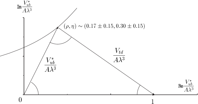
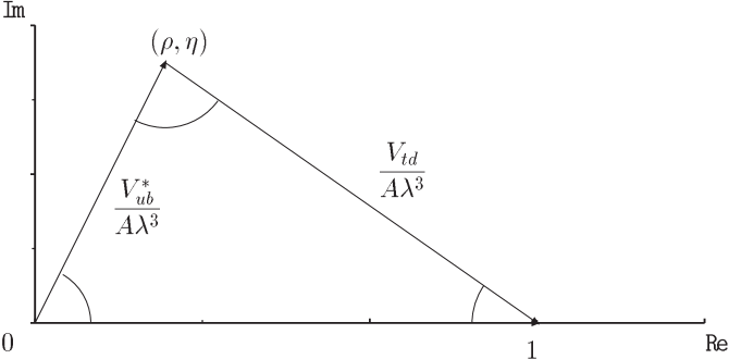
This relation identifies a triangle in the plane (see Fig. 1); the angles of this triangle are
Figure 1: The unitarity triangle.
measures of violation. The origin of the complex CKM phase
is still not clearly understood. It may be that it stems from the
short-distance dynamics [6] or extra dimensions (or something else)
[7].
1.4 Left-Right Symmetric Model
The fermion sector of the -symmetric
model [8] is the same as that of the SM; the boson sector involves the left
and right gauge bosons, whose interaction with quarks
is determined by the covariant derivative
(19)
and a suitable multiplet of the Higgs fields
interacts with quarks as follows:
(20)
where and the indices
denote generation. Vacuum expectation values (v.e.v.) of the Higgs fields can be taken to be
giving rise to the mass term of the form
where and .
Diagonalization of the mass matrices and can be made by the same token
as in the case of the SM:
where
(21)
are the mass eigenstates. Mixing in the left sector and
the elimination of arbitrariness in the choice of the matrices
and can be considered in the same way as in the case of the SM.
The additional interaction Lagrangian of the right currents
is expressed in terms of the mass eigenstates as follows:
(22)
where
(23)
In the case of two flavors,
In the case of flavors the number of independent -violating phases
is equal to .
2 Low-Energy Effective Lagrangian
It is well to recollect that any effective Lagrangian
derives from an expansion of the exact amplitudes at small external momenta.
Keeping only a few terms of such expansion (denote them by ), we find the
Lagrangian such that .
Now we turn to the consideration of the consequences of the -violating phase
for the hadronic physics.
This can be made in the two stages:
•
we construct the low-energy effective Lagrangian in terms of the quark fields,
where the CKM phase gives rise to the imaginary parts of the effective coupling constants,
represented by the Wilson coefficients;
•
using some model assumptions, we derive the expression for the Lagrangian in terms
of the meson fields.
As a result of the first stage of this evolution,
one obtains the effective Lagrangian [11]
(24)
which is a sum of local four–fermion operators ,
constructed with the light degrees of freedom,
(25)
where ,
and are color indices. The operators and
and the respective coefficients and are determined by the low-energy
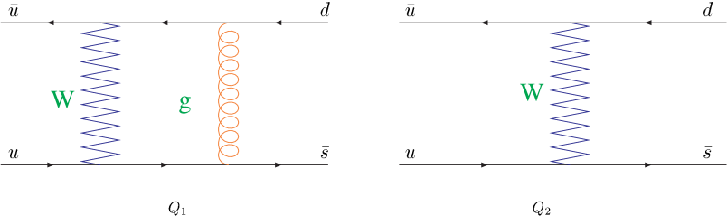
expansion of the diagrams in Fig. 3.
Figure 3: The diagrams for the short-distance processes giving rise to
the operators and in the effective Lagrangian (24).
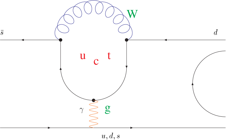
The remaining operators
(26)
come from the celebrated ’penguin’ diagram:
Figure 4: The ’penguin’ diagram.
The Wilson coefficients can be represented in the form
(27)
where
(28)
The -violating amplitudes are proportional to .
At the hadronic level, the effective Lagrangian is expressed in terms of the
The most general effective bosonic Lagrangian of the second order in derivatives,
with the same transformation properties and quantum numbers
as the short–distance Lagrangian, contains three terms [12]:
(29)
where the matrix
represents the octet of
currents at lowest order in derivatives,
is the quark
charge matrix,
projects onto the
transition []
and denotes the flavor trace of A.
The chiral couplings and measure the strength of the two
parts of the effective Lagrangian transforming as
and , respectively, under chiral rotations.
In the presence of electroweak interactions, the explicit breaking
of chiral symmetry generated by the quark charge matrix induces
the operator ,
transforming as under the chiral group.
(30)
The huge difference between these two couplings
shows the well–known enhancement of the octet transitions.
In the limit, the real parts of these constants are expressed
in terms of the Wilson coefficients as follows [13]:
(31)
The imaginary parts of them are responsible for -violating effects
and will be considered further.
With the effective weak Lagrangian at hand, it is very helpful to consider
the evolution of a meson system to the second order in the weak interaction.
3 Violation in System of Neutral Kaons
It has become a tradition333In this Section, we follow
[1, 14, 15] to begin a description of the system
with writing down the most general expression for -invariant Hamiltonian
where and are the eigenstates of the strong-interaction Hamiltonian
and the matrix is non-Hermitean.
However, it is well to recollect a derivation of this formula and formulate
the assumptions made in its derivation.
•
We consider weak interactions as a perturbation to the strong interactions.
•
We consider evolution of the eigenstates of the strong-interaction Hamiltonian
to the second order in the weak interaction and then search for the
effective Hamiltonian that would give the same evolution in the leading order
of perturbation theory [16].
The perturbation expansion of the matrix in the system
has the form
(32)
where , , and
is the weak-interaction Hamiltonian. To the second order in , we obtain
(33)
Making use of the Sokhotsky relations one can represent the transition
amplitudes as the matrix elements
of the effective Hamiltonian
(34)
where
(35)
Note that and . Thus the Hamiltonian
is related to the Hamiltonian of the weak interactions.
Eigenstates of this Hamiltonian are identified with the physical states
and , which are expressed through and
in terms of the parameter
(36)
the respective eigenvalues give the masses and widths
of the and mesons:
(37)
transformation exchanges and states:
(38)
The phase factor can be chosen arbitrarily, because any quantum-mechanical state
is defined up to a phase. However an interpretation of the matrix
elements and parameter depends on a particular choice of
the phase.
In the case , the parameters and are -odd,
whereas and are -even. Assuming that -odd parameters are small,
, we obtain
(39)
The formulas (37) agree with the experimental fact
if the sign of the square root is chosen so that
for
for
Experimental data indicate that ,
hence . Combining the above
formulas, we arrive at
(40)
for both and . (The assumption that
would give the phase factor instead of .)
3.1 Phase Convention
It is important and helpful to keep track of the phase arbitrariness
stemming from the fact that
The transformation rules induced by the rotation of the phase of the quark
(41)
are as follows:
Let the phases of the and be chosen so that the matrix of transformation
has the form
(we call it the ”default” phase convention).
It should be compared with the widely used Wu–Yang phase convention,
in which the phase of is set equal to zero. It should be noticed that
in the Wu–Yang phase convention the operator of transformation has the form
It should also be emphasized that the value as was
defined above is phase-dependent and so does not measure violation,
and the imaginary part of the effective weak Hamiltonian
is not associated with violation (and so it may be larger than real).
We adopt the ”default” phase convention. In this case
•
the quantities and are -odd;
•
and are -even;
•
is real;
Upon fixing a phase convention, the parameter makes
physical sense and can be related to measurable quantities; the -violating parameters
in the effective weak Hamiltonian are and .
3.2Mixing of and in the Standard Model
As has been demonstrated, such mixing is accounted for by the
effective weak Lagrangian.
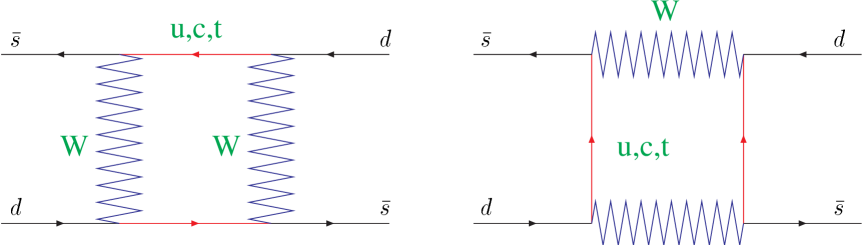
Let us consider the computation of the diagrams in Fig. 5 (giving the
transition amplitude ).
Gaillard and Lee in the pioneer work [17] obtained
(42)
Figure 5: transitions at the quark level.
where
(43)
Thus we obtain the effective Lagrangian
,
where444To simplify these expression it is well to use the unitarity condition
.
(44)
With the use of this Lagrangian the mass difference is readily obtained:
(45)
Now one should evaluate the matrix element
(46)
In early works, the matrix element was evaluated using the so called
”Vacuum Insertion Approximation”. The result is as follows:
(47)
The first computation of this matrix element was performed in the bag model
[18]; in was found that it is smaller from the naive expectation
of by a factor of 2. For this reason, the factor in the expression
(48)
is named ”the bag constant”. The computation of the bag factors presents
the major challenge in the calculations of -violating quantities
in nonleptonic reactions.
The short-distance contribution to comprises
of the total SM contribution:
(49)
where (in the approximation )555In the real
world, .
(50)
and the factor accounts for the corrections due to strong interactions, evaluated
in perturbative QCD.
The fact that indicates that the quark gives the dominant contribution
to the mass difference. The remaining are attributed to the long-distance
contribution (that is the contribution of the , etc
intermediate states in formula (35)),
which is extremely difficult to compute exactly.
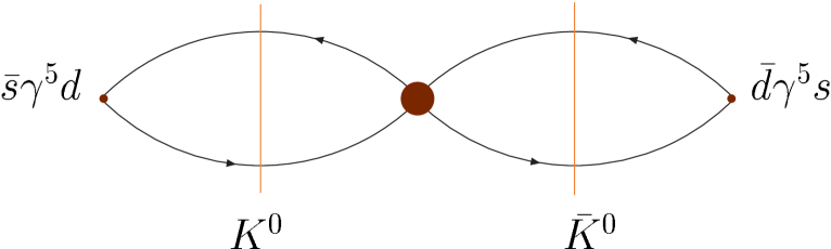
Figure 6: The transition in terms of the effective Lagrangian.
The estimates of the bag constant obtained in the lattice QCD and in
some models are
(51)
(52)
3.3Basic Formula for
In the above subsection we have considered in detail the determination of the real part
of the amplitude of the transition in terms of
the short-distance contribution (the second term in the expression (35)
for ) and the bag constant .
The imaginary part of this amplitude,
which appears in the expression (40) for ,
can be calculated by the same token.
In the case of imaginary part, one can safely neglect the long-distance contribution due
to low-lying intermediate states associated with the third
term in the expression (35) for ).
The result is
(53)
where
(54)
(here we have used the experimental value of , determined from ,
instead of the theoretical value (49)),
(55)
the short-distance corrections due to the strong interactions are absorbed
in the coefficients [21]
Formula (53) allows to set a limitation on the
-violating parameter of the SM from the experimental
limitations on (see Fig.(7)).
Figure 7: Formula (53) confines to lie in some vicinity of
the indicated hyperbola (see [5]). The combined set of
limitations makes the vertex of the unitarity triangle to lie within the indicated limits.
3.4 () Amplitudes
The decay amplitudes of the neutral Kaons in the channel with isospin
are defined by the matrix elements
(56)
where is the -wave phase shift of the scattering;
(57)
and
(58)
The properties of these amplitudes under the -transformation and
time reversal are seen from Table 2.
Table 2. Transformation properties of the isospin amplitudes. Transformation+——++—+—
It is seen that the amplitudes are -even, whereas the amplitudes
are -odd.
Using the relations
we obtain the expressions for the amplitudes
and :
(59)
describes the transitions with , whereas
describes the transitions with .
Assuming that the Hamiltonian for the transitions
contains only terms with quantum numbers and
(that is, it does not contain the terms with etc.),
we can use the Clebsch–Gordan coefficients
to obtain the amplitude
(60)
A comparison of the lifetimes of and leads one to a conclusion that the ratio
(61)
is very small, which is referred to as the long-standing ” problem”.
The experimental value .
The tree–level amplitudes generated
by the PT Lagrangian are:
(62)
Let us introduce the notation
(63)
We can now express the amplitudes , , and in terms of and the
parameter . For example,
Let us consider the experimentally measurable values
(65)
Proceeding as indicated above, we obtain
(66)
and a similar expression for .
Assuming that -violating parameters are small,
that is ,
we arrive at
(67)
where
In a similar way, one obtains
(68)
Let us introduce the parameters, which are conventionally used for a description of the
effects of violation:
(69)
Note that, in contrast to , the parameter is independent of
the phase convention. These values coincide only in the Wu–Yang phase convention.
In terms of the introduced parameters, we have
(70)
where
From the above it follows that
(71)
Note that is approximately real.
Using the short–distance Lagrangian, the –violating ratio
can be written as follows [22]:
(72)
where the quantities
(73)
contain the contributions from hadronic matrix elements
with isospin and
(74)
parameterizes isospin breaking corrections.
The factor enhances the relative weight of the
contributions.
The hadronic matrix elements
are usually parameterized
in terms of the bag parameters , which measure them
in units of their vacuum insertion approximation values.
In the SM, and turn out to
be dominated by the contributions from
the QCD penguin operator and
the electroweak penguin operator , respectively [23].
Thus, to a very good approximation,
can be written (up to global factors)
as [24, 25]
(75)
The isospin–breaking correction coming from - mixing
was originally estimated to be [26]. Together with the usual ansatz ,
this produces a large numerical cancellation
in (72) [27] leading to low values of
around .
A recent improved calculation of - mixing
at in PT has found the result [28]
(76)
This smaller number, slightly increases the naive estimate of .
∗This value depends crucially on the mass of the quark:
for MeV and for MeV
∗∗The most recent data:
(http://na48.web.cern.ch/NA48/Welcome/images/talks/win02/win02.pdf)
4Time-Reversal Invariance
Throughout this Section it is assumed that all the processes under consideration
are adequately described by some local quantum field theory, that is,
is an exact symmetry of the theory. In this case -violation
is equivalent to -violation and so we turn to the consideration of the
time-reversal invariance.
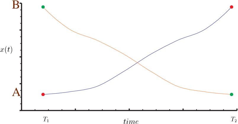
Figure 8: The reversal of time in classical mechanics.
Time-reversal invariance in the classical mechanics (Fig. 8):
motion from to
and
motion from to
are described with the same Hamiltonian
This is the case provided that .
Time-reversal invariance in the quantum mechanics:
evolution from to
and
evolution from to
are described with the same Hamiltonian
This is the case provided that .
Table 4. and transformations for various quantities. Action of these operators on the quantum-mechanical states is determined by the condition that
the - (or -)transformed states are characterized by the - (or -)transformed
(eigen)values of the respective operators.
Value
Notation
-transformed
-transformed
Comment
value
value
Coordinate
Momentum
Angular momentum
()
Spin
Like
Electric field
Magnetic field
Potential
Vector potential
Helicity
Transverse polarization∗
Triple correlation∗∗
∗A characteristic of a three-particle state, if at least one particle
has a nonzero spin.
∗∗A characteristic of a multiparticle state (number of particles
must be greater than 3).
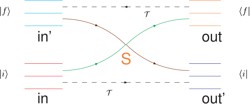
Figure 9: The reversal of time in the -matrix approach.
Time-reversal invariance in the -matrix approach:
The system described by the quantum field theory is invariant under
the time reversal if
•
the space of -states (’ket’-vectors) is isomorphic to the
space of states (’bra’-vectors)666This isomorphism is nothing
but assumption; however, it allows to consider the vectors from and
spaces as the vectors of the same Hilbert space ,
identified with .: ;
•
There exists (anti-unitary) operator of time reversal
which changes the signs of spins and momenta of all particles;
this condition can be cast in the form
for all vectors and ;
•
the transition from the state in the state
and the transition from the state to the state
are described with the same -matrix:
(77)
Having in mind that
(78)
we obtain the condition of -invariance in terms of the decay and scattering amplitudes:
(79)
In perturbation theory, the matrix is expanded in the coupling constant ,
which is assumed to be a small parameter:
(80)
Here is nothing but the interaction Lagrangian, ;
the unitarity of the matrix implies Hermiticity of the
interaction Lagrangian . Thus the -invariance condition
in the leading order of perturbation theory takes the form
(81)
To put it differently, if the complex-conjugated amplitude of the
transition between the states and differs in the leading order
of perturbation theory from the amplitude of the transition between
the states and then the dynamics of such system
is not invariant under the time reversal.
Let me illustrate this statement by considering the example of
the decay ; for definiteness, we consider the reference frame comoving
with the kaon. Let the average transverse777That is, transverse with respect to
the momenta of the outgoing particles polarization of the muon .
This is possible only if the probabilities of the decay
into the states with positive and negative transverse polarizations of the muon
differ from each other:
(82)
Note that the state
can be obtained from the state
as the result of the rotation by the angle of in the reaction plane.
For this reason,
(83)
The equations (82) and (83) imply the
conclusion as follows: if the transverse polarization of the muon
emerges in the first order of perturbation theory, then
(84)
that is, the dynamics is not invariant under the time reversal.
However, we should take into account the following reasoning.
Since the transverse polarization of the muon is determined by the
imaginary part of the decay amplitude, which does not vanish in higher
orders of perturbation theory due to unitarity condition,
the transverse polarization of the muon emerges in higher orders
even in the case of -even interactions.
Thus the transverse polarization of the muon in the decay can be caused by both electromagnetic and -odd interactions
(beyond the SM)
(85)
where is the electromagnetic contribution to the transverse
polarization of the muon and is the contribution of
the -odd (and, therefore -odd) interactions.
The -violating interactions can be accounted for by the imaginary parts of
the coupling constants in the effective quark–lepton Lagrangian
The interactions in (4) arise from new physics.
Nonvanishing imaginary parts in the effective coupling constants
gives rise to the imaginary parts of the form
factors
parameteriznig the matrix element of the decay ):
Figure 10: Diagrams giving a contribution to the imaginary part of the
amplitude of the decay .
Current limitations on the -violation parameters in various extensions of the SM
allow the transverse polarization of the muon in the decay
to be rather large: the left-right symmetric models
based on the symmetry group
with one doublet and two triplets of Higgs bosons
can give ,
supersymmetric models—,
leptoquark models—[34].
The respective -even contribution to the transverse polarization of the muon
is determined by the imaginary part of the decay amplitude (see Fig. 10)
and emerges in the second order in .
Straightforward computations of were made by several authors;
recent results [35] agree with each other and give the average value
(with the photon cutoff energy MeV).
The previous computations [36] are incomplete:
either diagrams in Fig. 10–10 or the diagrams in Fig. 10–10
were not taken into account.
A similar -even contribution to the correlation
in the decay is given by similar diagrams and has
the same order of magnitude [37].
4.1 and violation in the decays .
The imaginary part of the effective coupling constants , and
in the effective weak Lagrangian (29)
gives rise to the -violating effects in the decays .
The kinematical variables used to describe the decay
are as follows:
where ”3” is the ”odd” pion in either the or
decay mode. The slope parameters and
are defined by the formula for the differential probability of the decay:
(87)
The -violating quantities are as follows:
(88)
and
(89)
With the assumption that , the relevant amplitudes
can be expanded as follows:
(90)
From here on we restrict our attention to the slope asymmetry (89)
in the decay mode. As it usually is, this asymmetry is determined by the interplay
of (i) the imaginary parts of the parameters and , stemming from
the -odd effective weak Lagrangian (29) and (ii) the imaginary
part coming about the -even final-state interactions [38]:
(91)
An evaluation of the strong rescattering phases in the one-loop approximation
of the PT gives
(92)
The values , , , , , and
can be expanded in powers of the PT expansion parameter ,
where defines the momentum scale and MeV. In the case of -meson
decays, . In each order of the chiral expansion it is
helpful to isolate the and contributions to
, the latter contribution being suppressed by the factor .
The point is that, in the order , the neglect of the contribution
gives rise to the relations
and , which, in their turn imply that
However, the contribution does not vanish in the order
and so it dominates the total contribution. It is natural to assume that
it is enhanced by the factor (see 61) as compared to the contribution
in the order of the PT. The contribution is
suppressed by the PT expansion parameter as compared to
the contribution . The above reasoning is
summarized in Table 5.
Table 5. Various contributions to .
Order of PT
Numerical estimate
0
We see that the total contribution is dominated by the
contribution, which is times greater than
the contribution—due to vanishing of the contribution.
Maiani and Paver [38] assume that the enhancement factor may
run up to . Therewith, the conclusion by Bel’kov et al.[39] that the corrections increase the enhancement
factor by the order of magnitude appears, in view of the above reasoning,
highly questionable. It should also be noticed that the multi-Higgs models
allow a two-fold increase of the parameter as compared with
the SM prediction [40].
Acknowledgment: I am grateful to G.G. Volkov for stimulating discussions.
References
[1] T.-P. Cheng and L.-F. Li, ”Gauge Theory of Elementary Particle Physics”,
Claredon Press, Oxford, 1984.
[2] C. Itzykson and J.-B. Zuber, Quantum Field Theory, McGraw-Hill, 1980.
[9] A. Pich, Effective Field Theory, in
“Probing the Standard Model of Particle Interactions”, Proc.
1997 Les Houches Summer School, eds. R. Gupta et al.
(Elsevier, Amsterdam, 1999), Vol. II, p. 949.
[10] J. Gasser and H. Leutwyler, Nucl. Phys. B250, 465 (1985); A. Pich, Rep. Prog. Phys. 58, 563 (1995).
[11] L.B. Okun, ”Kvarki i leptony” (Quarks and leptons),
M.: Nauka (1990) (in Russian).
[12] G. Ecker, J. Kambor, D. Wyler, Nucl. Phys. B394, 101 (1993); G. Ecker, H. Neufeld, A. Pich, Nucl. Phys. B413, 321 (1994).
[13] W.A. Bardeen, A.J. Buras, and J.-M. Gérard, Nucl. Phys. B293, 787 (1987); A.J. Buras and J.-M. Gérard, Nucl. Phys. B264, 371 (1986); A. Pich, B. Guberina, and E. de Rafael, Nucl. Phys. B277, 197 (1986).
[14] L. Maiani, in The Second DANE Physics Handbook, L. Maiani, N. Pancheri, and N. Paver Eds., (SIS-Frascati 1995).
[15] Y.Nir, hep-ph/9911321.
[16] M. Gell-Mann and A. Pais, Rhys. Rev. 97, 1387 (1955).
![[Uncaptioned image]](/html/hep-ph/0204099/assets/x2.png)