Flavour mixing, gauge invariance and wave-function renormalisation

Abstract

We clarify some aspects of the LSZ formalism and wave function renormalisation for unstable particles in the presence of electroweak interactions when mixing and $CP$ violation are considered. We also analyse the renormalisation of the CKM mixing matrix which is closely related to wave function renormalisation. We critically review earlier attempts to define a set of “on-shell” wave function renormalisation constants. With the aid of an extensive use of the Nielsen identities complemented by explicit calculations we corroborate that the counter term for the CKM mixing matrix must be explicitly gauge independent and demonstrate that the commonly used prescription for the wave function renormalisation constants leads to gauge parameter dependent amplitudes, even if the CKM counter term is gauge invariant as required. We show that a proper LSZ-compliant prescription leads to gauge independent amplitudes. The resulting wave function renormalisation constants necessarily possess absorptive parts, but we verify that they comply with the expected requirements concerning $CP$ and $CPT$. The results obtained using this prescription are different (even at the level of the modulus squared of the amplitude) from the ones neglecting the absorptive parts in the case of top decay. The difference is numerically relevant.

PACS: 11.10Gh, 11.15.-q, 12.15 Lk, 12.15 Ff

1 Introduction

One of the pressing open problems in particle physics is to understand the origin of $CP$ violation phase and family mixing. In the minimal Standard Model (SM) the information about these quantities is encoded in the Cabibbo-Kobayashi-Maskawa (CKM) mixing matrix. In this work we shall denote this matrix by $K_{ij}$

As it is well known, some of the entries of this matrix are remarkably well measured, while others (such as the $K_{tb}$, $K_{ts}$ and $K_{td}$ elements) are poorly known and the only real experimental constraint come from the unitarity requirements. A lot of effort in the last decade has been invested in this particular problem and this dedication will continue in the foreseeable future aiming to a precision in the charged current sector comparable to the one already reached in the neutral sector. As a guidance, let us mention that the expected accuracy in $\sin 2\beta$ after LHCb is expected to be beyond the 1% level, and a comparable accuracy is expected by that time from the ongoing generation of experiments (BaBar, Belle) [1].

In the neutral sector it is totally mandatory to include electroweak radiative corrections to bring theory and experiment into agreement. Tree level results are incompatible with experiment by many standard deviations [2]. Obviously we are not there yet in the charged current sector, but in a few years electroweak radiative corrections will be required in the studies analysing the “unitarity” of the CKM matrix.

These corrections are of several types. With an on-shell scheme in mind, we need counter terms for the electric charge, Weinberg angle and wave-function renormalisation (wfr.) for the $W$ gauge boson. We shall also require wfr. for the external fermions and counter terms for the entries of the CKM matrix. The latter are in fact related in a way that will be described below [3]. Finally one needs to compute the 1PI vertex parts of the different processes one is interested in.

In the on-shell scheme, all counter terms can be expressed as combinations of self-energies [4]. These are standard and well known at one-loop in perturbation theory; in some cases, at least for the leading pieces, up to two-loop in the SM. However, a long standing controversy exists in the literature concerning what is the appropriate way to define both an external wfr. and CKM counter terms. The issue becomes involved because we are dealing with particles which are unstable (and therefore the self-energies develop branch cuts; even gauge dependent ones in the SM) and because of mixing.

Several proposals have been put forward in the literature to define appropriate counter terms both for the external legs and for the CKM matrix elements. The original prescription for wfr. diagonalizing the on-shell propagator was introduced in [5]. In [6] the wfr. “satisfying” the conditions of [5] were derived. However since [6] does not take care about the branch cuts present in the self-energies those results must be considered only consistent up to absorptive terms. Later it was realized [7] that the on-shell conditions defined in [5] where inconsistent and in fact impossible to satisfy for a minimal set of renormalisation constants due to the imaginary branch cuts present in the self-energies. The author of [7] circumvented this problem by introducing a prescription that de facto eliminates such branch cuts, but at the price of not diagonalizing the propagators in flavour space.

Ward identities based on the SU(2)_L gauge symmetry relate wfr. and counter terms for the CKM matrix elements [3]. In [8] it was seen that if the prescription of [6] was used in the counter terms for the CKM matrix elements, the results were in violation of gauge invariance. As we have just mentioned, the results in [6] do not deal properly with the absorptive terms appearing in the self-energies; which in addition happen to be gauge dependent. In spite of the problems with the prescription for the wfr. given in [6], the conclusions reached in [8] are correct: a necessary condition for gauge invariance of the physical amplitudes is that counter terms for the CKM matrix elements $K_{ij}$ are by themselves gauge independent. This condition is fulfilled by the CKM counter term proposed in [8] as it is in minimal subtraction [3], [9].

Other proposals to handle CKM renormalisation exist in the literature [9], [10] and [11]. In all these works either the external wfr. proposed originally in [6] or [7] are used, or the issue is sidestepped altogether. In either case the absorptive part of the self-energies (and even the absorptive part of the 1PI vertex part in one particular instance [10]) are not taken into account. As we shall see doing so leads to physical amplitudes — $S$-matrix elements— which are gauge dependent, and this irrespective of the method one uses to renormalise $K_{ij}$ provided the redefinition of $K_{ij}$ is gauge independent and preserves unitarity.

Due to the structure of the imaginary branch cuts it turns out however, that the gauge dependence present in the amplitude using the prescription of [7] cancels in the modulus squared of the physical $S$-matrix element in the SM. This cancellation has been checked numerically by the authors in [12]. In this work we shall provide analytical results showing that this cancellation is exact. However the gauge dependence remains at the level of the amplitude.

Is this acceptable? We do not think so. Diagrams contributing to the same physical process outside the SM electroweak sector may interfere with the SM amplitude and reveal the unwanted gauge dependence. Furthermore, gauge independent absorptive parts are also discarded by the prescription in [7]. These parts, contrary to the gauge dependent ones, do not drop in the squared amplitude as we shall show. In addition, one should not forget that the scheme in [7] does not deliver on-shell renormalised propagators that are diagonal in flavour space.

This work is dedicated to substantiate the above claims. We shall compute the gauge dependence of the absorptive parts in the self-energies and the vertex functions. We shall see how the requirements of gauge invariance and proper on-shell conditions (including exact diagonalisation in flavour space) single out a unique prescription for the wfr. The problem is presented in detail in the next section. The explicit expressions for the renormalisation constants are given in sections 3 and 4. Implementation for $W$ and top decay are shown in section 5. A technical discussion where extended use of the Nielsen identities has been done to extract the gauge dependence of all absorptive terms is presented in section 6 and it can be omitted by readers not interested in these details. In section 7 and 8 we return to $W$ and top decay to implement the previous results and finally we conclude in section 9.

2 Statement of the problem and its solution

We want to define an on-shell renormalisation scheme that guarantees the correct properties of the fermionic propagator in the $p^{2}\rightarrow m_{i}^{2}$ limit and at the same time renders the observable quantities calculated in such a scheme gauge parameter independent. In the first place up and down-type propagators have to be family diagonal on-shell. The conditions necessary for that purpose were first given by Aoki et. al. in [5]. Let us introduce some notation in order to write them down. We renormalise the bare fermion fields $\Psi_{0}$ and $\bar{\Psi}_{0}$ as

$$\Psi_{0}=Z^{\frac{1}{2}}\Psi\,,\qquad\bar{\Psi}_{0}=\bar{\Psi}\bar{Z}^{\frac{1}{2}}\,.$$ (2.1)

For reasons that will become clear along the discussion, we shall allow $Z$ and $\bar{Z}$ to be independent renormalisation constants. These renormalisation constants contain flavour, family and Dirac indices. We can decompose them into

$$Z^{\frac{1}{2}}=Z^{u\frac{1}{2}}\tau^{u}+Z^{d\frac{1}{2}}\tau^{d}\,,\qquad\bar{Z}^{\frac{1}{2}}=\bar{Z}^{u\frac{1}{2}}\tau^{u}+\bar{Z}^{d\frac{1}{2}}\tau^{d}\,,$$ (2.2)

with $\tau^{u}$ and $\tau^{d}$ the up and down flavour projectors and furthermore each piece in left and right chiral projectors, $L$ and $R$ respectively,

$$Z^{u\frac{1}{2}}=Z^{uL\frac{1}{2}}L+Z^{uR\frac{1}{2}}R\,,\qquad\bar{Z}^{u\frac{1}{2}}=\bar{Z}^{uL\frac{1}{2}}R+\bar{Z}^{uR\frac{1}{2}}L\,.$$ (2.3)

Analogous decompositions hold for $Z^{d\frac{1}{2}}$ and $\bar{Z}^{d\frac{1}{2}}$. Due to radiative corrections the propagator mixes fermion of different family indices. Namely

$$iS^{-1}\left(p\right)=\bar{Z}^{\frac{1}{2}}\left(\frac{{}}{{}}\not{p}-m-\delta m-\Sigma\left(p\right)\right)Z^{\frac{1}{2}}\,,$$

where the bare self-energy $\Sigma$ is non-diagonal and is given by $-i\Sigma=\sum$1PI. Within one-loop accuracy we can write $Z^{\frac{1}{2}}=1+\frac{1}{2}\delta Z$ etc. Introducing the family indices explicitly we have

$$iS_{ij}^{-1}\left(p\right)=\left(\not{p}-m_{i}\right)\delta_{ij}-\hat{\Sigma}_{ij}\left(p\right)\,,$$

where the one-loop renormalised self-energy is given by

$$\hat{\Sigma}_{ij}\left(p\right)=\Sigma_{ij}\left(p\right)-\frac{1}{2}\delta\bar{Z}_{ij}\left(\not{p}-m_{j}\right)-\frac{1}{2}\left(\not{p}-m_{i}\right)\delta Z_{ij}+\delta m_{i}\delta_{ij}\,.$$ (2.4)

Since we can project the above definition for up and down type-quarks, flavour indices will be dropped in the sequel and only will be restored when necessary. Recalling the following on-shell relations for Dirac spinors ($p^{2}\rightarrow m_{i}^{2}$)

$$\left(\not{p}-m_{i}\right)u_{i}^{\left(s\right)}\left(p\right) = 0\,,$$

$$\bar{u}_{i}^{\left(s\right)}\left(p\right)\left(\not{p}-m_{i}\right) = 0\,,$$

$$\left(\not{p}-m_{i}\right)v_{i}^{\left(s\right)}\left(-p\right) = 0\,,$$

$$\bar{v}_{i}^{\left(s\right)}\left(-p\right)\left(\not{p}-m_{i}\right) = 0\,,$$ (2.5)

the conditions [5] necessary to avoid mixing will be

$$\hat{\Sigma}_{ij}\left(p\right)u_{j}^{\left(s\right)}\left(p\right) = 0\,,\qquad(p^{2}\rightarrow m_{j}^{2})\,,\quad\mathrm{(incoming}\text{ }\mathrm{particle)}$$ (2.6)

$$\bar{v}_{i}^{\left(s\right)}\left(-p\right)\hat{\Sigma}_{ij}\left(p\right) = 0\,,\qquad(p^{2}\rightarrow m_{i}^{2})\,,\quad\mathrm{(incoming}\text{ }\mathrm{anti}\mathrm{-}\mathrm{particle)}$$ (2.7)

$$\bar{u}_{i}^{\left(s\right)}\left(p\right)\hat{\Sigma}_{ij}\left(p\right) = 0\,,\qquad(p^{2}\rightarrow m_{i}^{2})\,,\quad\mathrm{(outgoing}\text{ }\mathrm{particle)}$$ (2.8)

$$\hat{\Sigma}_{ij}\left(p\right)v_{j}^{\left(s\right)}\left(-p\right) = 0\,,\qquad(p^{2}\rightarrow m_{j}^{2})\,,\quad\mathrm{(outgoing}\text{ }\mathrm{anti}\mathrm{-}\mathrm{particle)}$$ (2.9)

where no summation over repeated indices is assumed and $i\neq j.$ These relations determine the non-diagonal parts of $Z$ and $\bar{Z}$ as will be proven in the next section. Here, as a side remark, let us point out that the need of different “incoming” and “outgoing” wfr. constants was already recognised in [13]. Nevertheless, that paper was unsuccessful in reconciling the on-shell prescription with the presence of absorptive terms in the self-energies. However, since its results are concerned with the leading contribution of an effective Lagrangian, no absorptive terms are present and therefore conclusions still hold.

To obtain the diagonal parts $Z_{ii},$ $\bar{Z}_{ii}$, and $\delta m_{i}$ one imposes mass pole and unit residue conditions (to be discussed below). Here it is worth to make one important comment regarding the above conditions. First of all we note that in the literature the relation

$$\bar{Z}^{\frac{1}{2}}=\gamma^{0}Z^{\frac{1}{2}\dagger}\gamma^{0}\,,$$ (2.10)

is taken for granted. This relation is tacitly assumed in [5] and explicitly required in [7]. Imposing Eq. (2.10) would guarantee hermiticity of the Lagrangian written in terms of the renormalised physical fields. However, we are at this point concerned with external leg renormalisation, for which it is perfectly possible to use a different set of renormalisation constants (even ones that do not respect the requirement (2.10)), while keeping the Lagrangian hermitian. In fact, using two sets of renormalisation constants is a standard practice in the on-shell scheme [4], so one should not be concerned by this fact per se. In case one is worried about the consistency of using a set of wfr. constants not satisfying (2.10) for the external legs while keeping a hermitian Lagrangian, it should be pointed out that there is a complete equivalence between the set of renormalisation constants we shall find out below and a treatment of the external legs where diagrams with self-energies (including mass counter terms) are inserted instead of the wfr. constants; provided, of course, that the mass counter term satisfy the on-shell condition. Proceeding in this way gives results identical to ours and different from those obtained using the wfr. proposed in [7], which do fulfil (2.10). Further consistency checks are presented in the following sections.

In any case, self-energies develop absorptive terms and this makes Eq. (2.10) incompatible with the diagonalizing conditions (2.6)-(2.9). Therefore in order to circumvent this problem one can give up diagonalisation conditions (2.6)-(2.9) or alternatively the hermiticity condition (2.10). The approach taken originally in [7] and works thereafter was the former alternative, while in this work we shall advocate the second one. The approach of [7] consists in dropping out absorptive terms from conditions (2.6)-(2.9). That is for $i\neq j$

$$\widetilde{Re}\left(\hat{\Sigma}_{ij}\left(p\right)\right)u_{j}^{\left(s\right)}\left(p\right) = 0\,,\qquad(p^{2}\rightarrow m_{j}^{2})\,,\quad\mathrm{(incoming}\text{ }\mathrm{particle)}$$

$$\bar{v}_{i}^{\left(s\right)}\left(-p\right)\widetilde{Re}\left(\hat{\Sigma}_{ij}\left(p\right)\right) = 0\,,\qquad(p^{2}\rightarrow m_{i}^{2})\,,\quad\mathrm{(incoming}\text{ }\mathrm{anti}\mathrm{-}\mathrm{particle)}$$

$$\bar{u}_{i}^{\left(s\right)}\left(p\right)\widetilde{Re}\left(\hat{\Sigma}_{ij}\left(p\right)\right) = 0\,,\qquad(p^{2}\rightarrow m_{i}^{2})\,,\quad\mathrm{(outgoing}\text{ }\mathrm{particle)}$$

$$\widetilde{Re}\left(\hat{\Sigma}_{ij}\left(p\right)\right)v_{j}^{\left(s\right)}\left(-p\right) = 0\,,\qquad(p^{2}\rightarrow m_{j}^{2})\,,\quad\mathrm{(outgoing}\text{ }\mathrm{anti}\mathrm{-}\mathrm{particle)}$$ (2.11)

where $\widetilde{Re}$ includes the real part of the logarithms arising in loop integrals appearing in the self-energies but not of the rest of coupling factors of the Feynmann diagram. This approach is compatible with the hermiticity condition (2.10) but on the other hand have several drawbacks. These drawbacks include

1. Since only the $\widetilde{Re}$ part of the self-energies enters into the diagonalizing conditions the on-shell propagator remains non-diagonal.

2. The very definition of $\widetilde{Re}$ relies heavily on the one-loop perturbative calculation where it is applied upon. In other words $\widetilde{Re}$ is not a proper function of its argument (in contrast to $Re$) and it is presumably cumbersome to implement in multi-loop calculations.

3. As it will become clear in next sections, the on-shell scheme based in the $\widetilde{Re}$ prescription leads to gauge parameter dependent physical amplitudes. The reason for this unwanted dependence is the dropping of absorptive gauge parameter dependent terms in the self-energies that are necessary to cancel absorptive terms appearing in the vertices. As mentioned in the introduction, in the SM, the gauge dependence drops in the modulus squared of the amplitude, but not in the amplitude itself and it could be eventually observable.

Once stated the unwanted features of the $\widetilde{Re}$ approach let us briefly state the consequences of dropping condition (2.10)

1. Conditions (2.6)-(2.9) readily determine the off-diagonal $Z$ and $\bar{Z}$ wfr. which coincide with the ones obtained using the $\widetilde{Re}$ prescription up to finite absorptive gauge parameter dependent terms.

2. The renormalised fermion propagator becomes exactly diagonal on-shell, unlike in the $\widetilde{Re}$ scheme.

3. Incoming and outgoing particles and anti-particles require different renormalisation constants when computing a physical amplitude. Annihilation of particles and creation of anti-particles are accompanied by the renormalisation constant $Z$, while creation of particles and annihilation of anti-particles are accompanied by the renormalisation constant $\bar{Z}$.

4. These constants $Z$ and $\bar{Z}$ are in what respects to their dispersive parts identical to the ones in [7]. They differ in their absorptive parts. This might suggest to the alert reader there could be problems with fundamental symmetries such as $CP$ or $CPT$. We shall discuss this issue at the end of the paper. Our conclusion is that everything works out consistently in this respect.

For explicit expressions for $Z$ and $\bar{Z}$ the reader should consult formulae (3.3), (3.4) and (4.10) in the next two sections. As an example how to implement them see section 5. The explicit dependence on the gauge parameter (for simplicity only the $W$ gauge parameter is considered) of the absorptive parts is given in section 7.

3 Off-diagonal wave-function renormalisation constants

This section is devoted to a detailed derivation of the off-diagonal renormalisation constants deriving entirely from the on-shell conditions (2.6)-(2.9) and allowing for $\bar{Z}^{\frac{1}{2}}\neq\gamma^{0}Z^{\frac{1}{2}\dagger}\gamma^{0}$. First of all we decompose the renormalised self-energy into all possible Dirac structures

$$\hat{\Sigma}_{ij}\left(p\right)=\not{p}\left(\hat{\Sigma}_{ij}^{\gamma R}\left(p^{2}\right)R+\hat{\Sigma}_{ij}^{\gamma L}\left(p^{2}\right)L\right)+\hat{\Sigma}_{ij}^{R}\left(p^{2}\right)R+\hat{\Sigma}_{ij}^{L}\left(p^{2}\right)L\,,$$ (3.1)

and use Eqs. (2.3), (2.4) and (3.1) to obtain

$$\hat{\Sigma}_{ij}\left(p\right) = \not{p}R\left(\Sigma_{ij}^{\gamma R}\left(p^{2}\right)-\frac{1}{2}\delta\bar{Z}_{ij}^{R}-\frac{1}{2}\delta Z_{ij}^{R}\right)+\not{p}L\left(\Sigma_{ij}^{\gamma L}\left(p^{2}\right)-\frac{1}{2}\delta\bar{Z}_{ij}^{L}-\frac{1}{2}\delta Z_{ij}^{L}\right)$$

$$+R\left(\Sigma_{ij}^{R}\left(p^{2}\right)+\frac{1}{2}\left(\delta\bar{Z}_{ij}^{L}m_{j}+m_{i}\delta Z_{ij}^{R}\right)+\delta_{ij}\delta m_{i}\right)+L\left(\Sigma_{ij}^{L}\left(p^{2}\right)+\frac{1}{2}\left(\delta\bar{Z}_{ij}^{R}m_{j}+m_{i}\delta Z_{ij}^{L}\right)+\delta_{ij}\delta m_{i}\right)\,.$$

Repeated indices are not summed over. Hence from Eqs. (3), (2.5) and (2.6) we obtain

$$\Sigma_{ij}^{\gamma R}\left(m_{j}^{2}\right)m_{j}-\frac{1}{2}\delta Z_{ij}^{R}m_{j}+\Sigma_{ij}^{L}\left(m_{j}^{2}\right)+\frac{1}{2}m_{i}\delta Z_{ij}^{L} = 0\,,$$

$$\Sigma_{ij}^{\gamma L}\left(m_{j}^{2}\right)m_{j}-\frac{1}{2}\delta Z_{ij}^{L}m_{j}+\Sigma_{ij}^{R}\left(m_{j}^{2}\right)+\frac{1}{2}m_{i}\delta Z_{ij}^{R} = 0\,.$$

Exactly the same relations are obtained from Eqs. (3), (2.5) and Eq. (2.9). Analogously, Eqs. (3), (2.5) and Eq. (2.7) (or Eq. (2.8)) lead to

$$m_{i}\Sigma_{ij}^{\gamma R}\left(m_{i}^{2}\right)-\frac{1}{2}m_{i}\delta\bar{Z}_{ij}^{R}+\Sigma_{ij}^{R}\left(m_{i}^{2}\right)+\frac{1}{2}\delta\bar{Z}_{ij}^{L}m_{j} = 0\,,$$

$$m_{i}\Sigma_{ij}^{\gamma L}\left(m_{i}^{2}\right)-\frac{1}{2}m_{i}\delta\bar{Z}_{ij}^{L}+\Sigma_{ij}^{L}\left(m_{i}^{2}\right)+\frac{1}{2}\delta\bar{Z}_{ij}^{R}m_{j} = 0\,.$$

Using the above expressions we immediately obtain

$$\delta Z_{ij}^{L} = \frac{2}{m_{j}^{2}-m_{i}^{2}}\left[\Sigma_{ij}^{\gamma R}\left(m_{j}^{2}\right)m_{i}m_{j}+\Sigma_{ij}^{\gamma L}\left(m_{j}^{2}\right)m_{j}^{2}+m_{i}\Sigma_{ij}^{L}\left(m_{j}^{2}\right)+\Sigma_{ij}^{R}\left(m_{j}^{2}\right)m_{j}\right]\,,$$

$$\delta Z_{ij}^{R} = \frac{2}{m_{j}^{2}-m_{i}^{2}}\left[\Sigma_{ij}^{\gamma L}\left(m_{j}^{2}\right)m_{i}m_{j}+\Sigma_{ij}^{\gamma R}\left(m_{j}^{2}\right)m_{j}^{2}+m_{i}\Sigma_{ij}^{R}\left(m_{j}^{2}\right)+\Sigma_{ij}^{L}\left(m_{j}^{2}\right)m_{j}\right]\,,$$ (3.3)

and

$$\delta\bar{Z}_{ij}^{L} = \frac{2}{m_{i}^{2}-m_{j}^{2}}\left[\Sigma_{ij}^{\gamma R}\left(m_{i}^{2}\right)m_{i}m_{j}+\Sigma_{ij}^{\gamma L}\left(m_{i}^{2}\right)m_{i}^{2}+m_{i}\Sigma_{ij}^{L}\left(m_{i}^{2}\right)+\Sigma_{ij}^{R}\left(m_{i}^{2}\right)m_{j}\right]\,,$$

$$\delta\bar{Z}_{ij}^{R} = \frac{2}{m_{i}^{2}-m_{j}^{2}}\left[\Sigma_{ij}^{\gamma L}\left(m_{i}^{2}\right)m_{i}m_{j}+\Sigma_{ij}^{\gamma R}\left(m_{i}^{2}\right)m_{i}^{2}+m_{i}\Sigma_{ij}^{R}\left(m_{i}^{2}\right)+\Sigma_{ij}^{L}\left(m_{i}^{2}\right)m_{j}\right]\,.$$ (3.4)

At the one-loop level in the SM we can define

$$\Sigma_{ij}^{R}\left(p^{2}\right)\equiv\Sigma_{ij}^{S}\left(p^{2}\right)m_{j}\,,\qquad\Sigma_{ij}^{L}\left(p^{2}\right)\equiv m_{i}\Sigma_{ij}^{S}\left(p^{2}\right)\,,$$

and therefore

$$\delta\bar{Z}_{ij}^{L}-\delta Z_{ij}^{L\dagger} = \frac{2}{m_{i}^{2}-m_{j}^{2}}\left\{\frac{{}}{{}}\left(\Sigma_{ij}^{\gamma R}\left(m_{i}^{2}\right)-\Sigma_{ji}^{\gamma R\ast}\left(m_{i}^{2}\right)\right)m_{i}m_{j}\right.+\left(\Sigma_{ij}^{\gamma L}\left(m_{i}^{2}\right)-\Sigma_{ji}^{\gamma L\ast}\left(m_{i}^{2}\right)\right)m_{i}^{2}$$

$$\left.+\left(m_{i}^{2}+m_{j}^{2}\right)\left(\frac{{}}{{}}\Sigma_{ij}^{S}\left(m_{i}^{2}\right)-\Sigma_{ji}^{S\ast}\left(m_{i}^{2}\right)\frac{{}}{{}}\right)\frac{{}}{{}}\right\}\neq 0\,,$$

and a similar relation holds for $\delta\bar{Z}_{ij}^{R}-\delta Z_{ij}^{R\dagger}.$ The above non-vanishing difference is due to the presence of branch cuts in the self-energies that invalidate the pseudo-hermiticity relation

$$\Sigma_{ij}\left(p\right)\neq\gamma^{0}\Sigma_{ij}^{\dagger}\left(p\right)\gamma^{0}\,.$$ (3.5)

Eq. (3.5) is assumed in [5] and if we, temporally, ignore those branch cut contributions our results reduces to the ones depicted in [6] or [7]. In the SM these branch cuts are generically gauge dependent as a cursory look to the appropriate integrals shows at once.

4 Diagonal wave-function renormalisation constants

Once the off-diagonal wfr. are obtained we focus our attention in the diagonal sector. Near the on-shell limit we can neglect the off-diagonal parts of the inverse propagator and write

$$iS_{ij}^{-1}\left(p\right)=\left(\not{p}-m_{i}-\hat{\Sigma}_{ii}\left(p\right)\right)\delta_{ij}=\left(\frac{{}}{{}}\not{p}\left(aL+bR\right)+cL+dR\frac{{}}{{}}\right)\delta_{ij}\,,$$ (4.1)

and therefore after some algebra

$$-iS_{ij}\left(p\right)=\frac{\not{p}\left(aL+bR\right)-dL-cR}{p^{2}ab-cd}\delta_{ij}\,,$$

in our case we have

$$a = 1-\Sigma_{ii}^{\gamma L}\left(p^{2}\right)+\frac{1}{2}\delta\bar{Z}_{ii}^{L}+\frac{1}{2}\delta Z_{ii}^{L}\,,$$

$$b = 1-\Sigma_{ii}^{\gamma R}\left(p^{2}\right)+\frac{1}{2}\delta\bar{Z}_{ii}^{R}+\frac{1}{2}\delta Z_{ii}^{R}\,,$$

$$c = -\Sigma_{ii}^{L}\left(p^{2}\right)-\left(1+\frac{1}{2}\delta\bar{Z}_{ii}^{R}+\frac{1}{2}\delta Z_{ii}^{L}\right)m_{i}-\delta m_{i}\,,$$

$$d = -\Sigma_{ii}^{R}\left(p^{2}\right)-\left(1+\frac{1}{2}\delta\bar{Z}_{ii}^{L}+\frac{1}{2}\delta Z_{ii}^{R}\right)m_{i}-\delta m_{i}\,.$$ (4.2)

In the limit $p^{2}\rightarrow m_{i}^{2}$ the chiral structures in the numerator has to cancel ($a\rightarrow b$ and $c\rightarrow d$), this requirement leads to

$$\delta\bar{Z}_{ii}^{R}-\delta\bar{Z}_{ii}^{L} = \Sigma_{ii}^{\gamma R}\left(m_{i}^{2}\right)-\Sigma_{ii}^{\gamma L}\left(m_{i}^{2}\right)+\frac{\Sigma_{ii}^{R}\left(m_{i}^{2}\right)-\Sigma_{ii}^{L}\left(m_{i}^{2}\right)}{m_{i}}\,,$$

$$\delta Z_{ii}^{R}-\delta Z_{ii}^{L} = \Sigma_{ii}^{\gamma R}\left(m_{i}^{2}\right)-\Sigma_{ii}^{\gamma L}\left(m_{i}^{2}\right)-\frac{\Sigma_{ii}^{R}\left(m_{i}^{2}\right)-\Sigma_{ii}^{L}\left(m_{i}^{2}\right)}{m_{i}}\,.$$ (4.3)

After this, we impose the inverse propagator to have a zero in its real part as $p^{2}\rightarrow m_{i}^{2}$

$$\lim_{p^{2}\rightarrow m_{i}^{2}}Re\left(p^{2}b-cda^{-1}\right)=0\,,$$ (4.4)

from where $\delta m_{i}$ is obtained

$$\delta m_{i}=-\frac{1}{2}Re\left\{m_{i}\Sigma_{ii}^{\gamma L}\left(m_{i}^{2}\right)+m_{i}\Sigma_{ii}^{\gamma R}+\Sigma_{ii}^{L}\left(m_{i}^{2}\right)+\Sigma_{ii}^{R}\left(m_{i}^{2}\right)\right\}\,.$$ (4.5)

This condition defines a mass and a width that agrees at the one-loop level with the ones given in [14], [15], [16] and [17]. Mass and width are defined as the real an imaginary parts of the propagator pole in the complex plane respectively. Note also that from Eqs. (4.2) (4.3) and (4.5) we have

$$\lim_{p^{2}\rightarrow m_{i}^{2}}\left(-ca^{-1}\right)=m_{i}+\frac{i}{2}Im\left(\Sigma_{ii}^{\gamma R}\left(m_{i}^{2}\right)m_{i}+\Sigma_{ii}^{\gamma L}\left(m_{i}^{2}\right)m_{i}+\Sigma_{ii}^{R}\left(m_{i}^{2}\right)+\Sigma_{ii}^{L}\left(m_{i}^{2}\right)\right)\,,$$ (4.6)

and therefore

$$\lim_{p^{2}\rightarrow m_{i}^{2}}\frac{\not{p}\left(aL+bR\right)-dL-cR}{p^{2}ab-cd}=\frac{\not{p}+m_{i}-i\Gamma/2}{im_{i}\Gamma}\,,$$

where the width is defined as

$$\Gamma\equiv-Im\left(\Sigma_{ii}^{\gamma R}\left(m_{i}^{2}\right)m_{i}+\Sigma_{ii}^{\gamma L}\left(m_{i}^{2}\right)m_{i}+\Sigma_{ii}^{R}\left(m_{i}^{2}\right)+\Sigma_{ii}^{L}\left(m_{i}^{2}\right)\right)\,.$$

This quantity is ultraviolet finite. In order to find the residue in the complex plane we expand the propagator around the physical mass obtaining for $p^{2}\sim m_{i}^{2}$

$$S_{ij}\left(p\right)=\frac{i\left[\not{p}+m_{i}-i\Gamma/2+\mathcal{O}\left(p^{2}-m_{i}^{2}\right)\right]}{im_{i}\Gamma+\left(p^{2}-m_{i}^{2}\right)a^{-1}\left[ab+m_{i}^{2}\left(a^{\prime}b+ab^{\prime}\right)-\left(c^{\prime}d+cd^{\prime}\right)\right]}+\mathcal{O}\left(\left(p^{2}-m_{i}^{2}\right)^{2}\right)\,,$$ (4.7)

where $a=b$ and $c=d$ are evaluated at $p^{2}=m_{i}^{2}$. Hereafter primed quantities denote derivatives with respect to $p^{2}$. $\mathcal{O}\left(\left(p^{2}-m_{i}^{2}\right)^{n}\right)$ stands for non-essential corrections of order $(p^{2}-m_{i}^{2})^{n}$. Note that the $\mathcal{O}\left(p^{2}-m_{i}^{2}\right)$ corrections in the numerator do not mix with the ones of the same order in the denominator since the first ones are of order $\Gamma^{-1}$ and the second ones are of order $\Gamma^{-2}.$ Taking into account these comments the unit residue condition amounts to requiring

$$1=\frac{a+b}{2}+m_{i}^{2}\left(a^{\prime}+b^{\prime}\right)+\left(m_{i}-i\Gamma/2\right)\left(c^{\prime}+d^{\prime}\right)\,,$$ (4.8)

from where

$$\frac{1}{2}\left(\delta\bar{Z}_{ii}^{L}+\delta\bar{Z}_{ii}^{R}\right) = \Sigma_{ii}^{\gamma L}\left(m_{i}^{2}\right)+\Sigma_{ii}^{\gamma R}\left(m_{i}^{2}\right)-\frac{1}{2}\left(\frac{{}}{{}}\delta Z_{ii}^{L}+\delta Z_{ii}^{R}\frac{{}}{{}}\right)+2m_{i}^{2}\left(\Sigma_{ii}^{\gamma L\prime}\left(m_{i}^{2}\right)+\Sigma_{ii}^{\gamma R\prime}\left(m_{i}^{2}\right)\right)$$ (4.9)

$$+2m_{i}\left(\frac{{}}{{}}\Sigma_{ii}^{L\prime}\left(m_{i}^{2}\right)+\Sigma_{ii}^{R\prime}\left(m_{i}^{2}\right)\frac{{}}{{}}\right)\,.$$

We have already required all the necessary conditions to fix the correct properties of the on-shell propagator but still there is some freedom left in the definition of the diagonal $Z$’s. This freedom can be expressed in terms of a set of finite coefficients $\alpha_{i}$ given by

$$\frac{1}{2}\left(\delta Z_{ii}^{L}+\delta Z_{ii}^{R}\right)=\frac{1}{2}\left(\delta\bar{Z}_{ii}^{L}+\delta\bar{Z}_{ii}^{R}\right)+\alpha_{i}\,.$$

Bearing in mind that ambiguity and using Eqs. (4.3) and (4.9) we obtain

$$\delta\bar{Z}_{ii}^{L} = \Sigma_{ii}^{\gamma L}\left(m_{i}^{2}\right)-X-\frac{\alpha_{i}}{2}+D\,,$$

$$\delta\bar{Z}_{ii}^{R} = \Sigma_{ii}^{\gamma R}\left(m_{i}^{2}\right)+X-\frac{\alpha_{i}}{2}+D\,,$$

$$\delta Z_{ii}^{L} = \Sigma_{ii}^{\gamma L}\left(m_{i}^{2}\right)+X+\frac{\alpha_{i}}{2}+D\,,$$

$$\delta Z_{ii}^{R} = \Sigma_{ii}^{\gamma R}\left(m_{i}^{2}\right)-X+\frac{\alpha_{i}}{2}+D\,,$$ (4.10)

where

$$X = \frac{1}{2}\frac{\Sigma_{ii}^{R}\left(m_{i}^{2}\right)-\Sigma_{ii}^{L}\left(m_{i}^{2}\right)}{m_{i}}\,,$$

$$D = m_{i}^{2}\left(\Sigma_{ii}^{\gamma L\prime}\left(m_{i}^{2}\right)+\Sigma_{ii}^{\gamma R\prime}\left(m_{i}^{2}\right)\right)+m_{i}\left(\frac{{}}{{}}\Sigma_{ii}^{L\prime}\left(m_{i}^{2}\right)+\Sigma_{ii}^{R\prime}\left(m_{i}^{2}\right)\frac{{}}{{}}\right)\,.$$

Note that since $X=0$ at the one-loop level and choosing $\alpha_{i}=0$ we obtain $\delta\bar{Z}_{ii}^{L}=\delta Z_{ii}^{L}$ and $\delta\bar{Z}_{ii}^{R}=\delta Z_{ii}^{R}.$ However we have the freedom to choose $\alpha_{i}\neq 0$. This does not affect the mass terms or neutral current couplings, but changes the charged coupling currents by multiplying the CKM matrix $K$ by diagonal matrices. These redefinitions do not change the physical observables provided the $\alpha_{i}$ are pure imaginary numbers. This ambiguity corresponds in perturbation theory to the well know freedom in phase redefinitions of the CKM matrix. Except for this last freedom, the on-shell conditions determine one unique solution, the one presented here, with $\bar{Z}^{\frac{1}{2}}\neq\gamma^{0}Z^{\frac{1}{2}\dagger}\gamma^{0}$.

5 W⁺ and top decay

Let us now apply the above mechanism to $W^{+}$ and top decay. We write

$$W^{+}\left(q\right) \rightarrow f_{i}\left(p_{1}\right)\bar{f}_{j}\left(p_{2}\right)\,,$$ (5.1)

$$f_{i}\left(p_{1}\right) \rightarrow W^{+}\left(q\right)f_{j}\left(p_{2}\right)\,,$$ (5.2)

where $f$ indicates particle and $\bar{f}$ anti-particle. The Latin indices are reserved for family indices. Leptonic and quark channels can be considered with the same notation, and confusion should not arise. For the process (5.1) there are at next-to-leading order two different type of Lorentz structures

$$M_{L}^{\left(1\right)} = \bar{u}_{i}\left(p_{1}\right)\not{\varepsilon}\left(q\right)Lv_{j}\left(p_{2}\right)\,,\qquad\left(L\leftrightarrow R\right)\,,$$

$$M_{L}^{\left(2\right)} = \bar{u}_{i}\left(p_{1}\right)Lv_{j}\left(p_{2}\right)p_{1}\cdot\varepsilon\left(q\right)\,,\qquad\left(L\leftrightarrow R\right)\,,$$ (5.3)

where $\varepsilon$ stands for the vector polarisation of the $W^{+}$. Equivalently for the process (5.2) we shall use

$$M_{L}^{\left(1\right)} = \bar{u}_{j}\left(p_{2}\right)\not{\varepsilon}^{\ast}\left(q\right)Lu_{i}\left(p_{1}\right)\,,\qquad\left(L\leftrightarrow R\right)\,,$$

$$M_{L}^{\left(2\right)} = \bar{u}_{j}\left(p_{2}\right)Lu_{i}\left(p_{1}\right)p_{1}\cdot\varepsilon^{\ast}\left(q\right)\,,\qquad\left(L\leftrightarrow R\right)\,.$$ (5.4)

The transition amplitude at tree level for the processes (5.1) and (5.2) is given by

$$\mathcal{M}_{0}=-\frac{eK_{ij}}{2s_{W}}M_{L}^{\left(1\right)}\,,$$

where Eq. (5.3) is used for $M_{L}^{\left(1\right)}$ in $W^{+}$ decay and Eq. (5.4) instead for $M_{L}^{\left(1\right)}$ in $t$ decay. The one-loop corrected transition amplitude can be written as

$$\mathcal{M}_{1} = -\frac{e}{2s_{W}}M_{L}^{\left(1\right)}\left[K_{ij}\left(1+\frac{\delta e}{e}-\frac{\delta s_{W}}{s_{W}}+\frac{1}{2}\delta Z_{W}\right)+\delta K_{ij}+\frac{1}{2}\sum_{r}\left(\delta\bar{Z}_{ir}^{Lu}K_{rj}+K_{ir}\delta Z_{rj}^{Ld}\right)\right]$$ (5.5)

$$-\frac{e}{2s_{W}}\left(\delta F_{L}^{\left(1\right)}M_{L}^{\left(1\right)}+M_{L}^{\left(2\right)}\delta F_{L}^{\left(2\right)}+M_{R}^{\left(1\right)}\delta F_{R}^{\left(1\right)}+M_{R}^{\left(2\right)}\delta F_{R}^{\left(2\right)}\right)\,.$$

In this expression $\delta F_{L,R}^{\left(1,2\right)}$ are the electroweak form factors coming from one-loop vertex diagrams. The renormalisation constants are given by

$$\frac{\delta e}{e} = -\frac{1}{2}\left[\left(\delta Z_{2}^{A}-\delta Z_{1}^{A}\right)+\delta Z_{2}^{A}\right]=-\frac{s_{W}}{c_{W}M_{Z}^{2}}\Pi^{ZA}\left(0\right)+\frac{1}{2}\frac{\partial\Pi^{AA}}{\partial k^{2}}\left(0\right)\,,$$

$$\frac{\delta s_{W}}{s_{W}} = -\frac{c_{W}^{2}}{2s_{W}^{2}}\left(\frac{\delta M_{W}^{2}}{M_{W}^{2}}-\frac{\delta M_{Z}^{2}}{M_{Z}^{2}}\right)=-\frac{c_{W}^{2}}{2s_{W}^{2}}Re\left(\frac{\Pi^{WW}\left(M_{W}^{2}\right)}{M_{W}^{2}}-\frac{\Pi^{ZZ}\left(M_{Z}^{2}\right)}{M_{Z}^{2}}\right)\,,$$

$$\delta Z_{W} = -\frac{\partial\Pi^{WW}}{\partial k^{2}}\left(M_{W}^{2}\right)\,,$$

and the fermionic wfr. constants are depicted in Eqs. (3.3), (3.4) and (4.10) where the indices $u$ or $d$ must be restored in the masses. The index $A$ refers to the photon field.

As for the $\delta K_{ij}$ renormalisation constants, a SU(2) Ward identity [8] fixes these counter terms to be

$$\delta K_{jk}=\frac{1}{4}\left[\left(\delta\hat{Z}^{uL}-\delta\hat{Z}^{uL\dagger}\right)K-K\left(\delta\hat{Z}^{dL}-\delta\hat{Z}^{dL\dagger}\right)\right]_{jk}\,,$$ (5.6)

where $\hat{Z}$ means that the wfr. constants appearing in the above expression are not necessarily the same ones used to renormalise and guarantee the proper on-shell residue for the external legs as already has been emphasised. One may, for instance, use minimal subtraction $Z$’s for the former.

We know [18] that the combination $\frac{\delta e}{e}-\frac{\delta s_{W}}{s_{W}}$ is gauge parameter independent. All the other vertex functions and renormalisation constants are gauge dependent. For the reasons stated in the introduction we want the amplitude (5.5) to be exactly gauge independent —not just its modulus— so the gauge dependence must cancel between all the remaining terms.

In the next section we shall make use of the Nielsen identities [19, 20, 21, 22] to determine that three of the form factors appearing in the vertex (5.5) are by themselves gauge independent, namely

$$\partial_{\xi}\delta F_{L}^{\left(2\right)}=\partial_{\xi}\delta F_{R}^{\left(1\right)}=\partial_{\xi}\delta F_{R}^{\left(2\right)}=0\,.$$

$\xi$ is the gauge-fixing parameter. We shall also see that the gauge dependence in the remaining form factor $\delta F_{L}^{\left(1\right)}$ cancels exactly with the one contained in $\delta Z_{W}$ and in $\delta Z$ and $\delta\bar{Z}$. Therefore to guarantee a gauge-fixing parameter independent amplitude $\delta K$ must be gauge independent as well.

The difficulties related to a proper definition of $\delta K$ were first pointed out in [8, 19], where it was realized that using the on-shell $Z$’s of [6] in Eq. (5.6) led to a gauge dependent $K$ and amplitude. They suggested a modification of the on-shell scheme based on a subtraction at $p^{2}=0$ for all flavours that ensured gauge independence. We want to stress that the choice for $\delta K$ is not unique and different choices may differ by gauge independent finite parts [12]. Note that the gauge independence of $\delta K$ is in contradistinction with the conclusions of [10] and in addition these authors have a non-unitary bare CKM matrix which does not respect the Ward identity.

As we shall see, if instead of using our prescription for $\delta Z$ and $\delta\bar{Z}$ one makes use of the wfr. constants of [7] to renormalise the external fermion legs, it turns out that the gauge cancellation dictated by the Nielsen identities does not actually take place in the amplitude. The culprits are of course the absorptive parts. These absorptive parts of the self-energies are absent in [7] due to the use of the $\widetilde{Re}$ prescription, which throws them away. Notice, though, that the vertex contribution has gauge dependent absorptive parts (calculated in the next section) and they remain in the final result.

One might think of absorbing these additional terms in the counter term for $\delta K$. This does not work. Indeed one can see from explicit calculations that wfr. constants decompose as

$$\delta Z^{Lu}=A^{uL}+iB^{uL}\,,\qquad\delta\bar{Z}^{Lu}=A^{uL\dagger}+iB^{uL\dagger}\,,\qquad\left(L\leftrightarrow R\text{, }u\leftrightarrow d\right)\,,$$ (5.7)

where the matrices $A$’s or $B$’s contain the dispersive and absorptive parts of the self-energies, respectively. Moreover if one substitutes back Eq. (5.7) into Eq. (5.5) one immediately sees that a necessary requirement allowing the $A^{u}$ and $A^{d}$ (respectively $B^{u}$ and $B^{d}$) contribution to be absorbed into a CKM matrix counter term of the form given in Eq. (5.6) is that $A^{u}$ and $A^{d}$ (respectively $B^{u}$ and $B^{d}$) were anti-hermitian (respectively hermitian) matrices. By direct inspection one can conclude that all $A$’s or $B$’s are neither hermitian nor anti-hermitian matrices and therefore any of such redefinitions are impossible unless one is willing to give up the unitarity of the bare $K$. A problem somewhat similar to that was encountered in [10] (but different, they did not consider absorptive parts at all, the inconsistency showed up already with the dispersive parts of the on-shell scheme of [6]).

It turns out that in the SM these gauge dependent absorptive parts, leading to a gauge dependent amplitude if they are dropped, do actually cancel, at least at the one-loop level, in the modulus of the $S$-matrix element. Thus at this level the use of $\widetilde{Re}$ is irrelevant. It is also shown in section 7 that gauge independent absorptive parts do survive even in the modulus of the amplitude for top or anti-top decay (and only in these cases). Therefore we have to conclude that the difference between using $\widetilde{Re}$, as advocated in [7], or not, as we do, is not just a semantic one. As we have seen such difference cannot be attributed to a finite renormalisation of $K$, provided the bare $K$ remains unitary as required by the Ward identity (5.6).

6 Nielsen Identities

In this section we derive in detail the gauge dependence of the vertex three-point function. It is therefore rather technical and it can be omitted by readers just interested in the physical conclusions. In order to have control on gauge dependence, a useful tool is provided by the so called Nielsen identities [20]. For such purpose besides the “classical” Lagrangian $\mathcal{L}_{\mathrm{SM}}$ we have to take into account the gauge fixing term $\mathcal{L}_{\mathrm{GF}}$, the Fadeev-Popov term $\mathcal{L}_{\mathrm{FP}}$ and source terms. Such source terms are the ones given by BRST variations of matter ($\bar{\eta}^{u},\eta^{u},\ldots$) and gauge fields together with Goldstone and ghost fields (not including anti-ghosts). We refer the reader to [4], [19] for notation and further explanations. We also include source terms ($\chi$) for the composite operators whose BRST variation generate $\mathcal{L}_{\mathrm{GF}}+\mathcal{L}_{\mathrm{FP}}.$ Schematically

$$\mathcal{L} = \mathcal{L}_{\mathrm{SM}}+\mathcal{L}_{\mathrm{GF}}+\mathcal{L}_{\mathrm{FP}}-\frac{1}{2\xi}\chi\left(\frac{{}}{{}}\left(\partial^{\mu}W_{\mu}^{-}-i\xi M_{W}G^{-}\right)\bar{c}^{+}+\left(\partial^{\mu}W_{\mu}^{+}-i\xi M_{W}G^{+}\right)\bar{c}^{-}\frac{{}}{{}}\right)$$

$$+\frac{ig}{\sqrt{2}}\bar{\eta}_{i}^{u}K_{ir}Ld_{r}-\frac{ig}{\sqrt{2}}\bar{c}^{+}\bar{d}_{r}K_{rj}^{\dagger}R\eta_{j}^{u}+\bar{s}_{i}^{u}u_{i}+\bar{u}_{j}s_{j}^{u}+\bar{s}_{i}^{d}d_{i}+\bar{d}_{j}s_{j}^{d}+\ldots\,,$$

where the ellipsis stands for the remaining source terms. The effective action, $\Gamma$, is introduced in the standard manner

$$\Gamma\left[\chi,\bar{\eta}^{u},\eta^{u},\bar{u}^{cl},u^{cl},\ldots\right]=W\left[\chi,\bar{\eta}^{u},\eta^{u},\bar{s}^{u},s^{u},\ldots\right]-\left(\bar{s}_{i}^{u}u_{i}^{cl}+\bar{u}_{j}^{cl}s_{j}^{u}+\bar{s}_{i}^{d}d_{i}^{cl}+\bar{d}_{j}^{cl}s_{j}^{d}+\ldots\right)\,,$$ (6.1)

with

$$e^{iW}=Z\left[\chi,\bar{\eta}^{u},\eta^{u},\bar{s}^{u},s^{u},\ldots\right]\equiv\int D\Phi\exp\left(i\mathcal{L}\right)\,.$$ (6.2)

From the above expressions and using BRST transformations we can extract the Nielsen identities for the three-point functions (see [20] for details)

$$\partial_{\xi}\Gamma_{W_{\mu}^{+}\bar{u}_{i}d_{j}} = -\Gamma_{\chi W_{\mu}^{+}\gamma_{W_{\alpha}}^{-}}\Gamma_{W_{\alpha}^{+}\bar{u}_{i}d_{j}}-\Gamma_{\chi\bar{u}_{i}\eta_{r}^{u}}\Gamma_{W_{\mu}^{+}\bar{u}_{r}d_{j}}-\Gamma_{W_{\mu}^{+}\bar{u}_{i}d_{r}}\Gamma_{\bar{\eta}_{r}^{d}d_{j}\chi}-\Gamma_{\chi W_{\mu}^{+}\gamma_{G_{\alpha}}^{-}}\Gamma_{G_{\alpha}^{+}\bar{u}_{i}d_{j}}$$ (6.3)

$$-\Gamma_{\chi\gamma_{G_{\alpha}}^{+}\bar{u}_{i}d_{j}}\Gamma_{G_{\alpha}^{-}W_{\mu}^{+}}-\Gamma_{\chi\gamma_{W_{\alpha}}^{+}\bar{u}_{i}d_{j}}\Gamma_{W_{\alpha}^{-}W_{\mu}^{+}}-\Gamma_{\chi W_{\mu}^{+}\bar{u}_{i}\eta_{r}^{d}}\Gamma_{\bar{d}_{r}d_{j}}-\Gamma_{\bar{u}_{i}u_{r}}\Gamma_{\chi W_{\mu}^{+}\bar{\eta}_{r}^{u}d_{j}}\,,$$

where we have omitted the momentum dependence and defined

$$\Gamma_{\chi\bar{u}_{i}\eta_{j}^{u}}\equiv\frac{\vec{\delta}}{\delta\chi}\frac{\vec{\delta}}{\delta\bar{u}_{i}^{cl}\left(p\right)}\frac{\delta}{\delta\eta_{j}^{u}\left(p\right)}\Gamma\,,\quad\Gamma_{\bar{\eta}_{i}^{u}u_{j}\chi}\equiv\frac{\delta}{\delta\bar{\eta}_{i}^{u}\left(p\right)}\frac{\vec{\delta}}{\delta u_{j}^{cl}\left(p\right)}\frac{\vec{\delta}}{\delta\chi}\Gamma\,.$$

In the rest of this section we shall evaluate the on-shell contributions to Eq. (6.3). Analogously we can also derive Nielsen identities for two-point functions

$$\partial_{\xi}\Gamma_{W_{\mu}^{+}W_{\beta}^{-}}^{\left(1\right)} = -2\left(\Gamma_{\chi W_{\mu}^{+}\gamma_{W_{\alpha}}^{-}}^{\left(1\right)}\Gamma_{W_{\alpha}^{+}W_{\beta}^{-}}+\Gamma_{\chi W_{\mu}^{+}\gamma_{G_{\alpha}}^{-}}^{\left(1\right)}\Gamma_{G_{\alpha}^{+}W_{\beta}^{-}}\right)\,,$$ (6.4)

$$\partial_{\xi}\Gamma_{W_{\mu}^{+}G_{\beta}^{-}}^{\left(1\right)} = -2\left(\Gamma_{\chi W_{\mu}^{+}\gamma_{W_{\alpha}}^{-}}^{\left(1\right)}\Gamma_{W_{\alpha}^{+}G_{\beta}^{-}}+\Gamma_{\chi W_{\mu}^{+}\gamma_{G_{\alpha}}^{-}}^{\left(1\right)}\Gamma_{G_{\alpha}^{+}G_{\beta}^{-}}\right)\,.$$ (6.5)

On-shell these reduce to

$$\Gamma_{\chi W^{+}\gamma_{W}^{-}}^{T\left(1\right)}\left(M_{W}^{2}\right)=-\frac{1}{2}\partial_{\xi}\left.\frac{\partial\Gamma_{W^{+}W^{-}}^{T\left(1\right)}}{\partial q^{2}}\left(q^{2}\right)\right|_{q^{2}=M_{W}^{2}}=\frac{1}{2}\partial_{\xi}\delta Z_{W}\,,\quad\Gamma_{\chi W^{+}\gamma_{G}^{-}}^{T\left(1\right)}\left(q\right)=0\,,$$ (6.6)

where the superscript $T$ refers to the transverse part and the superscript $(1)$ makes reference to the one-loop order correction.

Using these two sets of results and restricting Eq. (6.3) to the 1PI function appropriate for (on-shell) top-decay

$$\bar{u}_{u}\left(p_{i}\right)\epsilon^{\mu}\left(q\right)\partial_{\xi}\Gamma_{W_{\mu}^{+}\bar{u}_{i}d_{j}}^{\left(1\right)}v_{d}\left(-p_{j}\right)$$ (6.7)

$$= \frac{g}{\sqrt{2}}\bar{u}_{u}\left(p_{i}\right)\left\{\Gamma_{\chi\bar{u}_{i}\eta_{r}^{u}}K_{rj}\not{\epsilon}L+K_{ir}\not{\epsilon}L\Gamma_{\bar{\eta}_{r}^{d}d_{j}\chi}+\frac{1}{2}\partial_{\xi}\delta Z_{W}K_{ij}\not{\epsilon}L\right\}v_{d}\left(-p_{j}\right)\,.$$

At the one-loop level we also have the Nielsen identity

$$\partial_{\xi}\Sigma_{ij}^{u}\left(p\right)=\Gamma_{\chi\bar{u}_{i}\eta_{j}^{u}}^{\left(1\right)}\left(p\right)\left(\not{p}-m_{j}^{u}\right)+\left(\not{p}-m_{i}^{u}\right)\Gamma_{\bar{\eta}_{i}^{u}u_{j}\chi}^{\left(1\right)}\left(p\right)\,,$$ (6.8)

which is the fermionic counterpart of Eqs. (6.4) and (6.5). Similar relation holds interchanging $u\leftrightarrow d$. With the use of Eq. (6.8) and an analogous decomposition to Eq. (3.1) for $\Gamma$,

$$\Gamma_{\chi\bar{u}_{i}\eta_{j}^{u}}^{\left(1\right)}\left(p\right) = \not{p}\left(\Gamma_{\chi\bar{u}_{i}\eta_{j}^{u}}^{\gamma R\left(1\right)}\left(p^{2}\right)R+\Gamma_{\chi\bar{u}_{i}\eta_{j}^{u}}^{\gamma L\left(1\right)}\left(p^{2}\right)L\right)+\Gamma_{\chi\bar{u}_{i}\eta_{j}^{u}}^{R\left(1\right)}\left(p^{2}\right)R+\Gamma_{\chi\bar{u}_{i}\eta_{j}^{u}}^{L\left(1\right)}\left(p^{2}\right)L\,,$$

$$\Gamma_{\bar{\eta}_{i}^{u}u_{j}\chi}^{\left(1\right)}\left(p\right) = \not{p}\left(\Gamma_{\bar{\eta}_{i}^{u}u_{j}\chi}^{\gamma R\left(1\right)}\left(p^{2}\right)R+\Gamma_{\bar{\eta}_{i}^{u}u_{j}\chi}^{\gamma L\left(1\right)}\left(p^{2}\right)L\right)+\Gamma_{\bar{\eta}_{i}^{u}u_{j}\chi}^{R\left(1\right)}\left(p^{2}\right)R+\Gamma_{\bar{\eta}_{i}^{u}u_{j}\chi}^{L\left(1\right)}\left(p^{2}\right)L\,,$$ (6.9)

we obtain after equating Dirac structures

$$\partial_{\xi}\Sigma_{ij}^{u\gamma R}\left(p^{2}\right) = \Gamma_{\chi\bar{u}_{i}\eta_{j}^{u}}^{L\left(1\right)}\left(p^{2}\right)-m_{j}\Gamma_{\chi\bar{u}_{i}\eta_{j}^{u}}^{\gamma R\left(1\right)}\left(p^{2}\right)+\Gamma_{\bar{\eta}_{i}^{u}u_{j}\chi}^{R\left(1\right)}\left(p^{2}\right)-m_{i}\Gamma_{\bar{\eta}_{i}^{u}u_{j}\chi}^{\gamma R\left(1\right)}\left(p^{2}\right)\,,$$

$$\partial_{\xi}\Sigma_{ij}^{uR}\left(p^{2}\right) = p^{2}\Gamma_{\chi\bar{u}_{i}\eta_{j}^{u}}^{\gamma L\left(1\right)}\left(p^{2}\right)-m_{j}\Gamma_{\chi\bar{u}_{i}\eta_{j}^{u}}^{R\left(1\right)}\left(p^{2}\right)+p^{2}\Gamma_{\bar{\eta}_{i}^{u}u_{j}\chi}^{\gamma R\left(1\right)}\left(p^{2}\right)-m_{i}\Gamma_{\bar{\eta}_{i}^{u}u_{j}\chi}^{R\left(1\right)}\left(p^{2}\right)\,,$$ (6.10)

and analogous expressions exchanging $L\leftrightarrow R$ and $u\leftrightarrow d$. Moreover from Eqs. (6.7) and (6.9) we obtain

$$\bar{u}_{u}\left(p_{i}\right)\epsilon^{\mu}\left(q\right)\partial_{\xi}\Gamma_{W_{\mu}^{+}\bar{u}_{i}d_{j}}^{\left(1\right)}v_{d}\left(-p_{j}\right)=\frac{g}{\sqrt{2}}\left\{\frac{{}}{{}}\bar{u}_{u}\left(p_{i}\right)\left(m_{i}^{u}\Gamma_{\chi\bar{u}_{i}\eta_{r}^{u}}^{\gamma R\left(1\right)}\left(m_{i}^{u2}\right)+\Gamma_{\chi\bar{u}_{i}\eta_{r}^{u}}^{R\left(1\right)}\left(m_{i}^{u2}\right)\right)K_{rj}\not{\epsilon}Lv_{d}\left(-p_{j}\right)\right.+$$

$$\bar{u}_{u}\left(p_{i}\right)K_{ir}\not{\epsilon}L\left(m_{j}^{d}\Gamma_{\bar{\eta}_{r}^{d}d_{j}\chi}^{\gamma R\left(1\right)}\left(m_{j}^{d2}\right)+\Gamma_{\bar{\eta}_{r}^{d}d_{j}\chi}^{L\left(1\right)}\left(m_{j}^{d2}\right)\right)v_{d}\left(-p_{j}\right)+\left.\frac{1}{2}\partial_{\xi}\delta Z_{W}\bar{u}_{u}\left(p_{i}\right)K_{ij}\not{\epsilon}Lv_{d}\left(-p_{j}\right)\frac{{}}{{}}\right\}\,.$$ (6.11)

Using Eqs. (3.3), (3.4) and (6.10) one arrives at

$$m_{j}^{u}\Gamma_{\bar{\eta}_{i}^{u}u_{j}\chi}^{\gamma R\left(1\right)}\left(m_{j}^{u2}\right)+\Gamma_{\bar{\eta}_{i}^{u}u_{j}\chi}^{L\left(1\right)}\left(m_{j}^{u2}\right) = \frac{1}{2}\partial_{\xi}\delta Z_{ij}^{uL}\,,\quad\left(i\neq j\right)\,,$$ (6.12)

$$m_{i}^{u}\Gamma_{\chi\bar{u}_{i}\eta_{j}^{u}}^{\gamma R\left(1\right)}\left(m_{i}^{u2}\right)+\Gamma_{\chi\bar{u}_{i}\eta_{j}^{u}}^{R\left(1\right)}\left(m_{i}^{u2}\right) = \frac{1}{2}\partial_{\xi}\delta\bar{Z}_{ij}^{uL}\,,\quad\left(i\neq j\right)\,,$$ (6.13)

and once more similar relations hold exchanging $L\leftrightarrow R$ and $u\leftrightarrow d$. Notice that absorptive parts are present in the 1PI Green functions and hence in $\delta Z$ and $\delta\bar{Z}$ too. If we forget about such absorptive parts we would have pseudo-hermiticity. Namely

$$\Gamma_{\chi\bar{u}_{i}\eta_{j}^{u}}^{\left(1\right)}=\gamma^{0}\Gamma_{\bar{\eta}_{i}^{u}u_{j}\chi}^{\left(1\right)\dagger}\gamma^{0}\,,$$

where $\Gamma_{\bar{\eta}_{i}^{u}u_{j}\chi}^{\dagger}$ means complex conjugating $\Gamma_{\bar{\eta}_{i}^{u}u_{j}\chi}$ and interchanging both Dirac and family indices. However the imaginary branch cuts terms prevent the above relation to hold and then Eq. (2.10) does not hold.

At this point one might be tempted to plug expressions (6.12), (6.13) in Eq. (6.11). However such relations are obtained only in the restricted case $i\neq j$. For $i=j$ Eqs. (6.10) are insufficient to determine the combinations appearing in the lhs. of Eqs. (6.12), (6.13) and further information is required. That is also necessary even in the actual case where the rhs. of Eqs. (6.12), (6.13) are not singular at $m_{i}\rightarrow m_{j}$ [11]. In the rest of this section we shall proceed to calculate such diagonal combinations and as by product we shall also cross-check the results already obtained for the off-diagonal contributions and in addition produce some new ones.

By direct computation one generically finds

$$\Gamma_{\chi\bar{u}_{i}\eta_{j}^{u}}^{\left(1\right)} = \left(\frac{{}}{{}}\not{p}m_{i}^{u}B_{ij}^{u}\left(p^{2}\right)+C_{ij}^{u}\left(p^{2}\right)+A_{ij}^{u}\left(p^{2}\right)\frac{{}}{{}}\right)R\,,$$

$$\Gamma_{\bar{\eta}_{i}^{u}u_{j}\chi}^{\left(1\right)} = L\left(\frac{{}}{{}}\not{p}B_{ij}^{u}\left(p^{2}\right)m_{j}^{u}+C_{ij}^{u}\left(p^{2}\right)+A_{ij}^{u}\left(p^{2}\right)\frac{{}}{{}}\right)\,,$$ (6.14)

and analogous relations interchanging $u\leftrightarrow d.$ The $A$ function comes from the diagram containing a charged gauge boson propagator and $B$ and $C$ from the diagram containing a charged Goldstone boson propagator. From Eqs. (6.8) and (6.14) we obtain

$$\partial_{\xi}\Sigma_{ij}^{\gamma R}\left(p^{2}\right) = -2m_{i}B_{ij}\left(p^{2}\right)m_{j}\,,$$

$$\partial_{\xi}\Sigma_{ij}^{\gamma L}\left(p^{2}\right) = 2\left(\frac{{}}{{}}A_{ij}\left(p^{2}\right)+C_{ij}\left(p^{2}\right)\frac{{}}{{}}\right)\,,$$

$$\partial_{\xi}\Sigma_{ij}^{R}\left(p^{2}\right) = \left(\frac{{}}{{}}p^{2}B_{ij}\left(p^{2}\right)-C_{ij}\left(p^{2}\right)-A_{ij}\left(p^{2}\right)\frac{{}}{{}}\right)m_{j}\,,$$

$$\partial_{\xi}\Sigma_{ij}^{L}\left(p^{2}\right) = m_{i}\left(\frac{{}}{{}}p^{2}B_{ij}\left(p^{2}\right)-C_{ij}\left(p^{2}\right)-A_{ij}\left(p^{2}\right)\frac{{}}{{}}\right)\,.$$ (6.15)

The above system of equations is overdetermined and therefore some consistency identities between bare self-energies arise, namely

$$\partial_{\xi}\left(\frac{{}}{{}}m_{i}\Sigma_{ij}^{R}\left(p^{2}\right)-\Sigma_{ij}^{L}\left(p^{2}\right)m_{j}\frac{{}}{{}}\right)=0\,,$$ (6.16)

and

$$\partial_{\xi}\left(p^{2}\Sigma_{ij}^{\gamma R}\left(p^{2}\right)+\Sigma_{ij}^{\gamma L}\left(p^{2}\right)m_{i}m_{j}+m_{i}\Sigma_{ij}^{R}\left(p^{2}\right)+\Sigma_{ij}^{L}\left(p^{2}\right)m_{j}\right)=0\,.$$ (6.17)

These constrains must hold independently of any renormalisation scheme and we have checked them by direct computation. Actually the former trivially holds since, at least at the one-loop level in the SM,

$$m_{i}\Sigma_{ij}^{R}\left(p^{2}\right)-\Sigma_{ij}^{L}\left(p^{2}\right)m_{j}=0\,.$$ (6.18)

Finally, projecting Eq. (6.14) over spinors we also have

$$\bar{u}_{u}\left(p_{i}\right)\Gamma_{\chi\bar{u}_{i}\eta_{j}^{u}}^{\left(1\right)} = \bar{u}_{u}\left(p_{i}\right)\left(\frac{{}}{{}}m_{i}^{u2}B_{ij}^{u}\left(m_{i}^{u2}\right)+C_{ij}^{u}\left(m_{i}^{u2}\right)+A_{ij}^{u}\left(m_{i}^{u2}\right)\frac{{}}{{}}\right)R\,,$$

$$\Gamma_{\bar{\eta}_{i}^{d}d_{j}\chi}^{\left(1\right)}v_{d}\left(-p_{j}\right) = L\left(\frac{{}}{{}}B_{ij}^{d}\left(m_{j}^{d2}\right)m_{j}^{d2}+C_{ij}^{d}\left(m_{j}^{d2}\right)+A_{ij}^{d}\left(m_{j}^{d2}\right)\right)v_{d}\left(-p_{j}\right)\,.$$ (6.19)

The rhs. of the previous expressions can be evaluated in terms of the wfr. via the use of Eqs. (6.15)

$$\partial_{\xi} \left(m_{j}^{u}m_{i}^{u}\Sigma_{ij}^{u\gamma R}\left(p^{2}\right)+p^{2}\Sigma_{ij}^{u\gamma L}\left(p^{2}\right)+m_{j}^{u}\Sigma_{ij}^{uR}\left(p^{2}\right)+m_{i}^{u}\Sigma_{ij}^{uL}\left(p^{2}\right)\right)=$$ (6.21)

$$B_{ij}^{u}\left(p^{2}\right)\left(\frac{{}}{{}}p^{2}\left(m_{j}^{u2}+m_{i}^{u2}\right)-2m_{j}^{u2}m_{i}^{u2}\frac{{}}{{}}\right)+\left(2p^{2}-m_{j}^{u2}-m_{i}^{u2}\right)\left(A_{ij}^{u}\left(p^{2}\right)+C_{ij}^{u}\left(p^{2}\right)\frac{{}}{{}}\right)\,,$$

$$\partial_{\xi} \left(\Sigma_{ij}^{d\gamma R}\left(p^{2}\right)m_{i}^{d}m_{j}^{d}+\Sigma_{ij}^{d\gamma L}\left(p^{2}\right)p^{2}+m_{i}^{d}\Sigma_{ij}^{dL}\left(p^{2}\right)+\Sigma_{ij}^{dR}\left(p^{2}\right)m_{j}^{d}\right)=$$

$$B_{ij}^{d}\left(p^{2}\right)\left(\frac{{}}{{}}p^{2}\left(m_{i}^{d2}+m_{j}^{d2}\right)-2m_{i}^{d2}m_{j}^{d2}\right)+\left(2p^{2}-m_{i}^{d2}-m_{j}^{d2}\right)\left(\frac{{}}{{}}A_{ij}^{d}\left(p^{2}\right)+C_{ij}^{d}\left(p^{2}\right)\right)\,.$$

Hence using the off-diagonal wfr. expressions (3.3), (3.4) we re-obtain

$$\bar{u}_{u}\left(p_{i}\right)\frac{1}{2}\partial_{\xi}\delta\bar{Z}_{ij}^{uL}R=\bar{u}\left(p_{i}\right)\Gamma_{\chi\bar{u}_{i}\eta_{j}^{u}}^{\left(1\right)}\,,\qquad L\frac{1}{2}\partial_{\xi}\delta Z_{ij}^{dL}v_{d}\left(-p_{j}\right)=\Gamma_{\bar{\eta}_{i}^{d}d_{j}\chi}^{\left(1\right)}v_{d}\left(-p_{j}\right)\,.$$ (6.22)

For the diagonal wfr. we use Eqs. (4.10) together with (6.15) and (6.19) obtaining exactly the same result as in Eq. (6.22) with $i=j$ therein. Note however that since in Eq. (6.19) we have no derivatives with respect to $p^{2}$ obtaining Eq. (6.22) involves a subtle cancellation between the $p^{2}$ derivatives of the bare self-energies appearing in the definition of the diagonal wfr.

Before proceeding let us make a side remark concerning the regularity properties of the gauge derivative in Eqs. (6.21) and (6.21) in the limit $m_{i}\rightarrow m_{j}$. Note that evaluating Eq. (6.21) at $p^{2}=m_{i}^{u2}$ and Eq. (6.21) at $p^{2}=m_{j}^{d2},$ a global factor $\left(m_{i}^{u2}-m_{j}^{u2}\right)$ appears in the first equation and $\left(m_{j}^{d2}-m_{i}^{d2}\right)$ in the second one. Therefore it can be immediately seen that Nielsen identities together with the information provided by Eq. (6.14) assures the regularity of the gauge derivative for the off-diagonal wfr. constants when $m_{i}\rightarrow m_{j}$. Moreover we have seen that such limit is not only regular but also equal to the expression obtained from the diagonal wfr. which is not a priori obvious [8], [11].

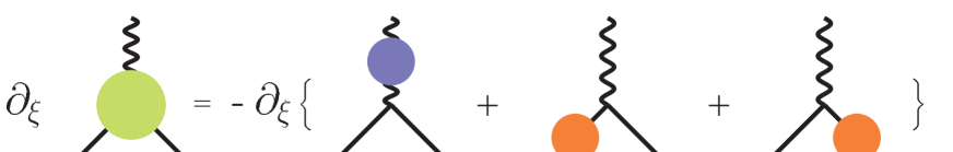
Figure 1: Pictorial representation of the on-shell Nielsen identity given by Eq.(LABEL:vertexgauge). The blobs in the lhs. represent bare one-loop contributions to the on-shell vertex and the blobs in the rhs. wfr. counter terms.

Replacing Eq. (6.22) in Eq. (6.7) we obtain

$$\partial_{\xi}\left(\bar{u}_{u}\left(p_{i}\right)\epsilon^{\mu}\left(q\right)\Gamma_{W_{\mu}^{+}\bar{u}_{i}d_{j}}^{\left(1\right)}v_{d}\left(-p_{j}\right)\right) = \frac{e}{2s_{W}}M_{L}^{\left(1\right)}\partial_{\xi}\left(\delta\bar{Z}_{ir}^{uL}K_{rj}+K_{ir}\delta Z_{rj}^{dL}+\delta Z_{W}K_{ij}\right)$$

$$= -\frac{e}{2s_{W}}\partial_{\xi}\left(M_{L}^{\left(1\right)}\delta F_{L}^{\left(1\right)}+M_{L}^{\left(2\right)}\delta F_{L}^{\left(2\right)}+M_{R}^{\left(1\right)}\delta F_{R}^{\left(1\right)}+M_{R}^{\left(2\right)}\delta F_{R}^{\left(2\right)}\right)\,,$$

where Eq. (5.5) and the gauge independence of the electric charge and Weinberg angle has been used in the last equality. In the previous expression $M_{L,R}^{\left(i\right)}$ are understood with the physical momenta $p_{1}$ and $p_{2}$ of Eq. (5.3) replaced by the diagrammatic momenta $p_{i}$ and $-p_{j}$ respectively. Note that Eq. (LABEL:vertexgauge) states that the gauge dependence of the on-shell bare one-loop vertex function cancels out the renormalisation counter terms appearing in Eq. (5.5) (see Fig. 1). This is one of the crucial results and special care should be taken not to ignore any of the absorptive parts —including those in the wfr. constants. As a consequence

$$\partial_{\xi}\mathcal{M}_{1}=-\frac{e}{2s_{W}}M_{L}^{\left(1\right)}\partial_{\xi}\delta K_{ij}\,,$$

and asking for a gauge independent amplitude the counter term for $K_{ij}$ must be separately gauge independent, as originally derived in [8].

Finally, since each structure $M_{L,R}^{\left(i\right)}$ must cancel separately we have that the Nielsen identities enforce

$$\partial_{\xi}\delta F_{L}^{\left(2\right)}=\partial_{\xi}\delta F_{R}^{\left(1\right)}=\partial_{\xi}\delta F_{R}^{\left(2\right)}=0\,.$$

7 Absorptive parts

Having determined in the previous section, thanks to an extensive use of the Nielsen identities, the gauge dependence of the different quantities appearing in top or $W$ decay in terms of the self-energies, we shall now proceed to list the absorptive parts of the wfr. constants, with special attention to their gauge dependence. The aim of this section is to state the differences between the wfr. constants given in our scheme and the ones in [7]. Recall that at one-loop such difference reduces to the absorptive ($\widetilde{Im}$) contribution to the $\delta Z$’s. In what concerns the gauge dependent part (with $\xi\geq 0$) the absorptive contribution ($\widetilde{Im}_{\xi}$) in the fermionic $\delta Z$’s amounts to

$$i\widetilde{Im}_{\xi}\left(\delta Z_{ij}^{uL}\right) = \sum_{h}\frac{iK_{ih}K_{hj}^{\dagger}}{8\pi v^{2}m_{j}^{u2}}\theta\left(m_{j}^{u}-m_{h}^{d}-\sqrt{\xi}M_{W}\right)\left(m_{j}^{u2}-m_{h}^{d2}-\xi M_{W}^{2}\right)$$

$$\times\sqrt{\left(\left(m_{j}^{u}-m_{h}^{d}\right)^{2}-\xi M_{W}^{2}\right)\left(\left(m_{j}^{u}+m_{h}^{d}\right)^{2}-\xi M_{W}^{2}\right)}\,,$$

$$i\widetilde{Im}_{\xi}\left(\delta\bar{Z}_{ij}^{uL}\right) = \sum_{h}\frac{iK_{ih}K_{hj}^{\dagger}}{8\pi v^{2}m_{i}^{u2}}\theta\left(m_{i}^{u}-m_{h}^{d}-\sqrt{\xi}M_{W}\right)\left(m_{i}^{u2}-m_{h}^{d2}-\xi M_{W}^{2}\right)$$

$$\times\sqrt{\left(\left(m_{i}^{u}-m_{h}^{d}\right)^{2}-\xi M_{W}^{2}\right)\left(\left(m_{i}^{u}+m_{h}^{d}\right)^{2}-\xi M_{W}^{2}\right)}\,,$$

$$\widetilde{Im}_{\xi}\left(\delta Z_{ij}^{uR}\right) = \widetilde{Im}_{\xi}\left(\delta\bar{Z}_{ij}^{uR}\right)=0\,,$$

where $\theta$ is the Heaviside function and $v$ is the Higgs vacuum expectation value. For the down $\delta Z$ we have the same formulae replacing $u\leftrightarrow d$ and $K\leftrightarrow K^{\dagger}.$ Note that using these results we can write

$$i\partial_{\xi}\widetilde{Im}\left[\sum_{r}\left(\delta\bar{Z}_{ir}^{uL}K_{rj}+K_{ir}\delta Z_{rj}^{dL}\right)+\delta Z_{W}K_{ij}\right]$$ (7.24)

$$= K_{ij}\partial_{\xi}\left\{\frac{i}{8\pi v^{2}}\left[\frac{1}{m_{i}^{u2}}\theta\left(m_{i}^{u}-m_{j}^{d}-\sqrt{\xi}M_{W}\right)\left(m_{i}^{u2}-m_{j}^{d2}-\xi M_{W}^{2}\right)\right.\right.$$

$$+\left.\frac{1}{m_{j}^{d2}}\theta\left(m_{j}^{d}-m_{i}^{u}-\sqrt{\xi}M_{W}\right)\left(m_{j}^{d2}-m_{i}^{u2}-\xi M_{W}^{2}\right)\frac{{}}{{}}\right]$$

$$\times\left.\sqrt{\left(\left(m_{j}^{d}-m_{i}^{u}\right)^{2}-\xi M_{W}^{2}\right)\left(\left(m_{j}^{d}+m_{i}^{u}\right)^{2}-\xi M_{W}^{2}\right)}+i\widetilde{Im}_{\xi}\left(\delta Z_{W}\right)\frac{{}}{{}}\right\}\,.$$

In the case $\left|m_{i}^{u}-m_{j}^{d}\right|\leq\sqrt{\xi}M_{W}$ the above expression reduces to

$$\partial_{\xi}\sum_{r}\widetilde{Im}\left(\delta\bar{Z}_{ir}^{uL}K_{rj}+K_{ir}\delta Z_{rj}^{dL}\right)=0\,,$$ (7.25)

while for $\left|m_{i}^{u}-m_{j}^{d}\right|\geq\sqrt{\xi}M_{W}$ we have

$$i\partial_{\xi}\sum_{r}\widetilde{Im}\left(\delta\bar{Z}_{ir}^{uL}K_{rj}+K_{ir}\delta Z_{rj}^{dL}\right)=$$

$$K_{ij}\partial_{\xi}\left\{\frac{i}{4\pi v^{2}}\frac{\left|m_{i}^{u2}-m_{j}^{d2}\right|-\xi M_{W}^{2}}{m_{i}^{u2}+m_{j}^{d2}+\left|m_{i}^{u2}-m_{j}^{d2}\right|}\sqrt{\left(\left(m_{j}^{d}-m_{i}^{u}\right)^{2}-\xi M_{W}^{2}\right)\left(\left(m_{j}^{d}+m_{i}^{u}\right)^{2}-\xi M_{W}^{2}\right)}\right\}\,.$$ (7.26)

Moreover the $\xi$-dependent absorptive contribution to $\delta Z_{W}$ ($\widetilde{Im}_{\xi}\left(\delta Z_{W}\right)$) has no dependence in quark masses since the diagram with a fermion loop is gauge independent. Because of that we can conclude that the derivative in Eq. (7.24) does not vanish. Defining $\Delta_{ij}$ as the difference between the vertex observable calculated in our scheme and the same in the scheme using $\widetilde{Re}$ we have

$$\Delta_{ij}\sim\left|K_{ij}\right|^{2}\mathrm{Re}\left(i\widetilde{Im}\delta Z_{W}\right)+\mathrm{Re}\left\{iK_{ij}^{\ast}\sum_{r}\left[\widetilde{Im}\left(\delta\bar{Z}_{ir}^{uL}\right)K_{rj}+K_{ir}\widetilde{Im}\left(\delta Z_{rj}^{dL}\right)\right]\right\}\,.$$

In the case of $\delta Z_{W}$ one can easily check that $\widetilde{Im}\left(\delta Z_{W}\right)=\mathrm{Im}\left(\delta Z_{W}\right)$ obtaining

$$\Delta_{ij}\sim\mathrm{Re}\left\{iK_{ij}^{\ast}\sum_{r}\left[\widetilde{Im}\left(\delta\bar{Z}_{ir}^{uL}\right)K_{rj}+K_{ir}\widetilde{Im}\left(\delta Z_{rj}^{dL}\right)\right]\right\}\,.$$ (7.27)

Thus from Eqs. (7.25), (7.26) and (7.27) we immediately obtain

$$\partial_{\xi}\Delta_{ij}\sim\mathrm{Re}\left\{iK_{ij}^{\ast}\sum_{r}\left[\partial_{\xi}\widetilde{Im}\left(\delta\bar{Z}_{ir}^{uL}\right)K_{rj}+K_{ir}\partial_{\xi}\widetilde{Im}\left(\delta Z_{rj}^{dL}\right)\right]\right\}=0\,.$$ (7.28)

However gauge independent absorptive parts, included if our prescription is used but not if one uses the one of [7] which makes use of the $\widetilde{Re}$, do contribute to Eq. (7.27). In order to see that we can take $\xi=1$ obtaining for the physical values of the masses

$$\widetilde{Im}_{\xi=1}\left(\delta Z_{rj}^{dL}\right) = 0\,,$$

$$\widetilde{Im}_{\xi=1}\left(\delta\bar{Z}_{ir}^{uL}\right) = \sum_{h}\frac{K_{ih}K_{hr}^{\dagger}}{8\pi v^{2}m_{i}^{u2}}\frac{\theta\left(m_{i}^{u}-m_{h}^{d}-M_{W}\right)}{m_{i}^{u2}-m_{r}^{u2}}\sqrt{\left(m_{i}^{u2}-\left(M_{W}-m_{h}^{d}\right)^{2}\right)\left(m_{i}^{u2}-\left(M_{W}+m_{h}^{d}\right)^{2}\right)}$$ (7.29)

$$\times\left(\frac{1}{2}\left(m_{r}^{u2}+m_{h}^{d2}+2M_{W}^{2}\right)\left(m_{i}^{u2}+m_{h}^{2d}-M_{W}^{2}\right)-\left(m_{i}^{u2}+m_{r}^{u2}\right)m_{h}^{d2}\right)\,,$$

where only the results for $i\neq j$ have been presented. Note that $\widetilde{Im}_{\xi=1}\left(\delta\bar{Z}_{ir}^{uL}\right)\neq 0$ only when $i=3$, that is when the renormalised up-particle is a top. In addition, since the $m_{r}^{u2}$ dependence in Eq. (7.29) does not vanish, CKM phases do not disappear from Eq. (7.27) and therefore

$$\Delta_{3j}\sim\mathrm{Re}\left\{iK_{3j}^{\ast}\sum_{r}\left[\widetilde{Im}\left(\delta\bar{Z}_{3r}^{uL}\right)K_{rj}+K_{3r}\widetilde{Im}\left(\delta Z_{rj}^{dL}\right)\right]\right\}\neq 0\,.$$ (7.30)

Eqs. (7.28) and (7.30) show that even though the difference $\Delta_{3j}$ is gauge independent, does not actually vanish. There are genuine gauge independent pieces that contribute not only to the amplitude, but also to the observable. As discussed these additional pieces cannot be absorbed by a redefinition of $K_{ij}$. Numerically such gauge independent corrections amounts roughly to $\Delta_{3j}\simeq 5\times 10^{-3}O_{\mathrm{tree}}$ where $O_{\mathrm{tree}}$ is the observable quantity calculated at leading order.

8 CP violation and CPT invariance

In this section we want to show that using wfr. constants that do not verify a pseudo-hermiticity condition does not lead to any unwanted pathologies. In particular: (a) No new sources of $CP$ violation appear besides the ones already present in the SM. (b) The total width of particles and anti-particles coincide, thus verifying the $CPT$ theorem. Let us start with the latter, which is not completely obvious since not all external particles and anti-particles are renormalised with the same constant due to the different absorptive parts.

The optical theorem asserts that

$$\Gamma_{t}\sim\sum_{f}\int d\Pi_{f}\left|M\left(t^{\left(\hat{n}\right)}\left(p\right)\rightarrow f\right)\right|^{2} = 2\mathrm{Im}\left[M\left(t^{\left(\hat{n}\right)}\left(p\right)\rightarrow t^{\left(\hat{n}\right)}\left(p\right)\right)\right]\,,$$ (8.31)

$$\Gamma_{\bar{t}}\sim\sum_{f}\int d\Pi_{f}\left|M\left(\bar{t}^{\left(\hat{n}\right)}\left(p\right)\rightarrow f\right)\right|^{2} = 2\mathrm{Im}\left[M\left(\bar{t}^{\left(\hat{n}\right)}\left(p\right)\rightarrow\bar{t}^{\left(\hat{n}\right)}\left(p\right)\right)\right]\,,$$ (8.32)

where we have consider, just as an example, top ($t^{\left(\hat{n}\right)}\left(p\right)$) and anti-top ($\bar{t}^{\left(\hat{n}\right)}\left(p\right)$) decay, with $p$ and $\hat{n}$ being their momentum and polarisation. Recalling that the incoming fermion and outgoing anti-fermion spinors are renormalised with a common constant (see Eq. (2.1)) as are the outgoing fermion and incoming anti-fermion ones, it is immediate to see that

$$M\left(t^{\left(\hat{n}\right)}\left(p\right)\rightarrow t^{\left(\hat{n}\right)}\left(p\right)\right) = \bar{u}^{\left(\hat{n}\right)}\left(p\right)A_{33}\left(p\right)u^{\left(\hat{n}\right)}\left(p\right)\,,$$

$$M\left(\bar{t}^{\left(\hat{n}\right)}\left(p\right)\rightarrow\bar{t}^{\left(\hat{n}\right)}\left(p\right)\right) = -\bar{v}^{\left(\hat{n}\right)}\left(p\right)A_{33}\left(-p\right)v^{\left(\hat{n}\right)}\left(p\right)\,,$$

where the minus sign comes from an interchange of two fermion operators and where the subscripts in $A$ indicate family indices. Using the fact that

$$u^{\left(\hat{n}\right)}\left(p\right)\otimes\bar{u}^{\left(\hat{n}\right)}\left(p\right)=\frac{\not{p}+m}{2m}\frac{1+\gamma^{5}\not{n}}{2}\,,\qquad-v^{\left(\hat{n}\right)}\left(p\right)\otimes\bar{v}^{\left(\hat{n}\right)}\left(p\right)=\frac{-\not{p}+m}{2m}\frac{1+\gamma^{5}\not{n}}{2}\,,$$

with $n=\frac{1}{\sqrt{\left(p^{0}\right)^{2}-\left(\vec{p}\cdot\hat{n}\right)^{2}}}\left(\vec{p}\cdot\hat{n},p^{0}\hat{n}\right)$ being the polarisation four-vector and performing some elementary manipulations we obtain

$$\bar{u}^{\left(\hat{n}\right)}\left(p\right)A_{33}\left(p\right)u^{\left(\hat{n}\right)}\left(p\right) = Tr\left[\left(\frac{\not{p}+m}{2m}\frac{1+\gamma^{5}\not{n}}{2}\right)\left(a\left(p^{2}\right)\not{p}L+b\left(p^{2}\right)\not{p}R+c\left(p^{2}\right)L+d\left(p^{2}\right)R\right)\right]$$

$$= \frac{1}{4}Tr\left\{\frac{\not{p}+m}{2m}\left[\left(a\left(p^{2}\right)+b\left(p^{2}\right)\right)\not{p}+c\left(p^{2}\right)+d\left(p^{2}\right)\right]\right\}$$

$$= \frac{1}{4}Tr\left\{\frac{-\not{p}+m}{2m}\left[-\left(a\left(p^{2}\right)+b\left(p^{2}\right)\right)\not{p}+c\left(p^{2}\right)+d\left(p^{2}\right)\right]\right\}$$

$$= Tr\left[\frac{-\not{p}+m}{2m}\frac{1+\gamma^{5}\not{n}}{2}\left(-a\left(p^{2}\right)\not{p}L-b\left(p^{2}\right)\not{p}R+c\left(p^{2}\right)L+d\left(p^{2}\right)R\right)\right]$$

$$= -\bar{v}^{\left(\hat{n}\right)}\left(p\right)A_{33}\left(-p\right)v^{\left(\hat{n}\right)}\left(p\right)\,,$$

where we have decomposed $A_{33}\left(p\right)$ into its most general Dirac structure. We thus conclude the equality between Eqs. (8.31) and (8.32) verifying that the lifetimes of top and anti-top are identical. The detailed form of the wfr. constants, or whether they have absorptive parts or not, does not play any role.

Even thought total decay widths for top and anti-top are identical the partial ones need not to if $CP$ violation is present and some compensation between different processes must take place. This issue is discussed in detail in [23]. Here we shall show that when $K=K^{\ast}$ the $CP$ invariance of the Lagrangian manifests itself in a zero asymmetry between the partial differential decay rate of top and its $CP$ conjugate process. The fact that the external renormalisation constants have dispersive parts does not alter this conclusion. This is of course expected on rather general grounds, so the following discussion has to be taken really as a verification that no unexpected difficulties arise.

To illustrate this point let us consider the top decay channel $t\left(p_{1}\right)\rightarrow W^{+}\left(p_{1}-p_{2}\right)+b\left(p_{2}\right)$ and its $CP$ conjugate process $\bar{t}\left(\tilde{p}_{1}\right)\rightarrow W^{-}\left(\tilde{p}_{1}-\tilde{p}_{2}\right)+b\left(\tilde{p}_{2}\right).$ Let us note the respective amplitudes by $\mathcal{A}$ and $\mathcal{B}$ which are given as

$$\mathcal{A} = \varepsilon^{\mu}\bar{u}^{\left(s_{2}\right)}\left(p_{2}\right)A_{\mu}u^{\left(s_{1}\right)}\left(p_{1}\right)\,,$$

$$\mathcal{B} = -\tilde{\varepsilon}^{\mu}\bar{v}^{\left(s_{1}\right)}\left(\tilde{p}_{1}\right)B_{\mu}v^{\left(s_{2}\right)}\left(\tilde{p}_{2}\right)\,,$$

where $\tilde{a}^{\mu}=a_{\mu}=\left(a^{0},-a^{i}\right)$ for any four-vector. Considering contributions up to including next-to-leading corrections we have

$$A_{\mu} = -i\frac{e}{\sqrt{2}s_{W}}\left[\left(\bar{Z}^{\frac{1}{2}bL}K^{\dagger}Z^{\frac{1}{2}tL}+K^{\dagger}\delta_{V}+\delta K^{\dagger}\right)\gamma_{\mu}L+\delta F_{\mu}\right]\,,$$

$$B_{\mu} = -i\frac{e}{\sqrt{2}s_{W}}\left[\left(\bar{Z}^{\frac{1}{2}tL}KZ^{\frac{1}{2}bL}+K\delta_{V}+\delta K\right)\gamma_{\mu}L+\delta G_{\mu}\right]\,,$$

with $\delta_{V}$ $=\frac{\delta e}{e}-\frac{\delta s_{W}}{s_{W}}+\frac{1}{2}\delta Z_{W}$ and $\delta F_{\mu}$ and $\delta G_{\mu}$ are given by the one-loop diagrams. From a direct computation it can be seen that if $K=K^{\ast}$ this implies

$$\bar{Z}^{\frac{1}{2}L}=\left(Z^{\frac{1}{2}L}\right)^{T}\,,\quad\bar{Z}^{\frac{1}{2}R}=\left(Z^{\frac{1}{2}R}\right)^{T}\,,\quad\tilde{\varepsilon}^{\mu}\delta G_{\mu}=\varepsilon^{\mu}\gamma^{2}\delta F_{\mu}^{T}\gamma^{2}\,,$$ (8.33)

where the superscript $T$ means transposition with respect to all indices (family indices in the case of $Z^{\frac{1}{2}L}$ and $Z^{\frac{1}{2}R}$ and Dirac indices in the case of $\delta F_{\mu}$ ). Using

$$i\gamma^{2}\bar{u}^{\left(s\right)T}\left(p\right)=sv^{\left(s\right)}\left(\tilde{p}\right)\,,\qquad u^{\left(s\right)T}\left(p\right)i\gamma^{2}=-s\bar{v}^{\left(s\right)}\left(\tilde{p}\right)\,,$$

where $s=\pm 1$, depending on the spin direction in the $\hat{z}$ axis, we obtain

$$\mathcal{A} = \frac{-ie}{\sqrt{2}s_{W}}\varepsilon^{\mu}\bar{u}^{\left(s_{2}\right)}\left(p_{2}\right)\left[\left(\bar{Z}^{\frac{1}{2}bL}K^{\dagger}Z^{\frac{1}{2}tL}+K^{\dagger}\delta_{V}+\delta K^{\dagger}\right)\gamma_{\mu}L+\delta F_{\mu}\right]u^{\left(s_{1}\right)}\left(p_{1}\right)$$

$$= \frac{-ie}{\sqrt{2}s_{W}}\varepsilon^{\mu}u^{\left(s_{1}\right)T}\left(p_{1}\right)\left[L\left(\left(Z^{\frac{1}{2}tL}\right)^{T}K^{\ast}\left(\bar{Z}^{\frac{1}{2}bL}\right)^{T}+K^{\ast}\delta_{V}+\delta K^{\ast}\right)\gamma_{\mu}^{T}+\delta F_{\mu}^{T}\right]\bar{u}^{\left(s_{2}\right)T}\left(p_{2}\right)$$

$$= \frac{-s_{1}s_{2}ie}{\sqrt{2}s_{W}}\varepsilon^{\mu}\bar{v}^{\left(s_{1}\right)}\left(\tilde{p}_{1}\right)\gamma^{2}\left[L\left(\left(Z^{\frac{1}{2}tL}\right)^{T}K^{\ast}\left(\bar{Z}^{\frac{1}{2}bL}\right)^{T}+K^{\ast}\delta_{V}+\delta K^{\ast}\right)\gamma_{\mu}^{T}+\delta F_{\mu}^{T}\right]\gamma^{2}v^{\left(s_{2}\right)}\left(\tilde{p}_{2}\right)$$

$$= \frac{-s_{1}s_{2}ie}{\sqrt{2}s_{W}}\varepsilon^{\mu}\bar{v}^{\left(s_{1}\right)}\left(\tilde{p}_{1}\right)\left[\left(\left(Z^{\frac{1}{2}tL}\right)^{T}K^{\ast}\left(\bar{Z}^{\frac{1}{2}bL}\right)^{T}+K^{\ast}\delta_{V}+\delta K^{\ast}\right)\gamma_{\mu}^{\dagger}L+\gamma^{2}\delta F_{\mu}^{T}\gamma^{2}\right]v^{\left(s_{2}\right)}\left(\tilde{p}_{2}\right)\,,$$

now using Eq. (8.33) we see that if no $CP$ violating phases are present in the CKM matrix $K$ (and therefore neither in $\delta K,$ Eq. (5.6)) we obtain that $\mathcal{A}=-s_{1}s_{2}\mathcal{B}$ and thus

$$\left|\mathcal{A}\right|^{2}=\left|\mathcal{B}\right|^{2}\,.$$

Note again that when $CP$ violating phases are present we can expect in general non-vanishing phase-space dependent asymmetries for the different channels. Once we sum over all channels and integrate over the final state phase space a compensation must take place as we have seen guaranteed by unitarity and $CPT$ invariance. Using a set of wfr. constants with absorptive parts as advocated here (and required by gauge invariance) leads to different results than using the prescription originally advocated in [7], in particular using Eq. (7.30) for $K\neq K^{\ast}$ we expect $\Delta_{3j}^{\left(t~{}decay\right)}-\Delta_{3j}^{\left(\bar{t}~{}decay\right)}\neq 0$.

9 Conclusions

Let us recapitulate our main results. We hope, first of all, to have convinced the reader that there is a problem with what appears to be the commonly accepted prescription for dealing with wave function renormalisation when mixing is present. The situation is even further complicated by the appearance of $CP$ violating phases. The problem has a twofold aspect. On the one hand the prescription of [7] does not diagonalise the propagator matrix in flavour space in what respects to the absorptive parts. On the other hand it yields gauge dependent amplitudes, albeit gauge independent modulus squared of the amplitudes. This is not satisfactory: interference with e.g. strong phases may reveal an unacceptable gauge dependence.

The only solution is to accept wfr. constants that do not satisfy a pseudo-hermiticity condition due to the presence of the absorptive parts, which are neglected in [7]. This immediately brings about some gauge independent absorptive parts which appear even in the modulus squared amplitude and which are neglected in the treatment of [7]. Furthermore, these parts (and the gauge dependent ones) cannot be absorbed in unitary redefinitions of the CKM matrix which are the only ones allowed by Ward identities. We have checked that —although unconventional— the presence of the absorptive parts in the wfr. constants is perfectly compatible with basic tenets of field theory and the Standard Model. Numerically we have found the differences to be important, at the order of the half per cent. Small, but relevant in the future. This information will be relevant to extract the experimental values of the CKM mixing matrix.

Traditionally, wave function renormalisation seems to have been the “poor relative” in the Standard Model renormalisation program. We have seen here that it is important on two counts. First because it is related to the counter terms for the CKM mixing matrix, although the on-shell values for wave function constants cannot be directly used there. Second because they are crucial to obtain gauge independent $S$ matrix elements and observables. While using our wfr. constants (but not the ones in [7]) for the external legs is strictly equivalent to considering reducible diagrams (with on-shell mass counter terms) the former procedure is considerably more practical.

References

[1] S. Amato et al. [LHCb Collaboration],
CERN-LHCC-98-4.
[2] A. Pich, arXiv:hep-ph/9711279.
[3] C. Balzereit, T. Mannel and B. Plumper,
Eur. Phys. J. C 9, 197 (1999) [arXiv:hep-ph/9810350].