Abstract

We present a contribution of higher order to neutrino–electron scattering that is a charged-current counterpart of both the anomalous axial-vector triangle and possible non-standard interaction contributions. It arises in the standard model with massive neutrinos, and renormalizes the nondiagonal axial-vector form-factor at low energies. We show that, due to the small size of radiative corrections, the neutrino–electron scattering still provides a discovery potential for some of the non-standard neutrino interactions proposed in the literature.

1 Introduction

We have reached the time where the advance in neutrino experiments enables quite accurate global fits on the leptonic mixing angles. Simultaneously, the advent of the neutrino masses gives hope to infer on the specific departures from the standard model (SM). In this sense we explore here a further discovery potential of the neutrino–electron scattering.

Ever since the earliest studies of the neutrino–electron scattering, this particular process remained in a focus of interest. The underlying diagonal $\nu$–$e$ interaction density is provided by the SM, which at energies much lower than $M_{W}$ gives

$$\mathcal{H}^{\text{diag}}(x)=\frac{G_{F}}{\sqrt{2}}\,\bar{e}\gamma^{\mu}(g_{V}-g_{A}\gamma_{5})e\,\bar{\nu}\gamma_{\mu}(1-\gamma_{5})\nu\;.$$ (1)

Here $g_{V}$ and $g_{A}$ are the SM couplings, where both charged and neutral current contribute for $\nu=\nu_{e}\,$ ($g_{V}=1/2+2\sin^{2}\theta_{W}$, $g_{A}=1/2$), whereas there is only neutral current contribution for $\nu=\nu_{\mu},\nu_{\tau}$ ($g_{V}=-1/2+2\sin^{2}\theta_{W}$, $g_{A}=-1/2$).

On the experimental side, the results for atmospheric neutrinos [1], in conjunction with the results from the Sudbury Neutrino Observatory (SNO) [2], show that the disappearance of one neutrino flavour (such as reported by the SuperKamiokande) is accompanied by the appearance of another. Such conversion of the neutrino species appears naturally if neutrinos have nonvanishing masses.

The neutrino masses imply at least a minimal extension of the SM, where a mismatch in diagonalizing mass matrices of charged and neutral leptons results in a $3\times 3$ flavour mixing matrix. It enters the leptonic charged current interactions, that generalizes the interaction (1) to the nondiagonal $\nu_{H}$ $\leftrightarrow$ $\nu_{L}$ transition

$$\mathcal{H}^{\text{non-diag}}_{\text{rad}}(x)=\frac{G_{F}}{\sqrt{2}}\,\bar{e}\gamma^{\mu}(f_{V}-f_{A}\gamma_{5})e\,\bar{\nu}_{L}\gamma_{\mu}(1-\gamma_{5})\nu_{H}\;.$$ (2)

Here, $\nu_{H}$ and $\nu_{L}$ are just generic labels for neutrino mass eigenstates. The form of Eq. (2) explicates the lepton conversion in the neutrino sector, rather than in the charged lepton sector.

In a more ambitious approach, where one attempts to explain neutrino masses, one faces the theories that include non-standard interactions (NSI) of neutrinos with matter [3]. In particular, we focus here to the neutrino conversion via left- ($L=(1-\gamma_{5})/2$) and right-handed ($R=(1+\gamma_{5})/2$) neutral current NSI of the form

$$\mathcal{H}_{\text{eff}}^{\text{NSI}}=\sqrt{2}G_{F}\big{[}\epsilon^{eL}_{\alpha\beta}\bar{e}\gamma^{\mu}Le+\epsilon^{eR}_{\alpha\beta}\bar{e}\gamma^{\mu}Re\big{]}\big{[}\bar{\nu}_{\alpha}\gamma_{\mu}(1-\gamma_{5})\nu_{\beta}\big{]}$$ (3)

explored further by [4, 5]. Such neutral current interactions may be confused with the higher loop effects of the charged currents, comprised in the $f_{V,A}$ terms in (2).

In the next section we will present a novel contribution to the axial form-factor $f_{A}$ in (2) arising from the charged current transition at the two-loop level. In Sect. 3 we will demonstrate that, due to the fact that the SM based loop contribution is small, there is ample space left for a discovery of certain NSI contributions.

2 The Neutrino Conversion in the Presence of the Axial Coupling to Electrons

Let us recall a heuristic role of an early study of radiative corrections to the neutrino–electron scattering. The radiative correction at order $\alpha^{2}$ displayed on Fig. 1 generates an infinite nonrenormalizable contribution to the $g_{A}$ form-factor of the diagonal interaction (1). Adler [6] observed this infinite radiative correction to $\nu_{l}l$ scattering by embedding the triangle diagram calculated by Rosenberg [7] into the next loop. In present day terminology, the axial triangle anomaly resides in the neutral current piece of the $\nu$–$e$ interaction displayed on Fig. 1(b).

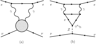
Figure 1: Radiative corrections of order $\alpha^{2}$ displayed in the 1PI blob (a), contain a nonrenormalizable triangle diagram in the axial-vector part of the neutral current amplitude (b).

Among possible remedies for infinities proposed by Adler [6], the idea to add to the electron triangle on Fig. 1(b) the muon triangle with opposite sign, survived in its essence to the present day. The quantum numbers assigned to the SM fermion representations confirmed such cancellation for each generation of fundamental fermions, and this anomaly cancelation remained as a guiding principle for model building ever since.

In addition to this piece of the neutrino axial current for which nature took care by itself, neutrino masses invoke another contribution at same order of $\alpha^{2}$, that is finite. Up to our knowledge, this extra part to which we turn in this paper, is novel in the literature.

Let us look how such counterpart to original Adler’s contribution sets in for massive neutrinos. In this case, the neutrino flavour eigenstates are mixtures of the mass eigenstates, described by the leptonic 3$\times$3 unitary matrix (nowadays dubbed the Pontecorvo-Maki-Nakagawa-Sakata $U_{\text{PMNS}}$ matrix [8, 9], in analogy to the Cabibbo-Kobayashi-Maskawa matrix in the quark sector of the Standard model)

$$\left(\begin{array}[]{c}\nu_{e}\\ \nu_{\mu}\\ \nu_{\tau}\end{array}\right)=\left(\begin{array}[]{ccc}U_{e1}&U_{e2}&U_{e3}\\ U_{\mu 1}&U_{\mu 2}&U_{\mu 3}\\ U_{\tau 1}&U_{\tau 2}&U_{\tau 3}\end{array}\right)\left(\begin{array}[]{c}\nu_{1}\\ \nu_{2}\\ \nu_{3}\end{array}\right)\equiv U_{\text{PMNS}}\left(\begin{array}[]{c}\nu_{1}\\ \nu_{2}\\ \nu_{3}\end{array}\right)\;.$$ (4)

Note that the flavour violation induced by the PMNS mixing (similarly to the one by the CKM mixing) does not affect the renormalizability of the electroweak theory. Thus, a safe evaluation of the quantum-loop corrections is possible. Recently, we employed this framework in calculating lepton-flavour violating annihilation of muonium [10, 11]. Now we consider the radiative corrections which will allow for the neutrino conversion via the two-photon exchange similar to Fig. 1(a).

Since the PMNS mixing affects only the charged current, our starting point is the tree diagram displayed on Fig. 2(a). Its two-photon radiative corrections will result in Fig. 2(b) as the nondiagonal counterpart to Fig. 1.

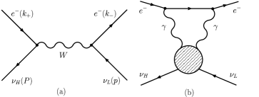
Figure 2: Tree-level Feynman diagram (a), describing the nondiagonal neutrino–electron interaction, and the photonic-loop diagram (b) induced by the $\nu_{H}\nu_{L}\gamma\gamma$ vertex (the shaded circle).

The referent tree-level amplitude corresponding to the diagram on Fig. 2(a) reads (after a Fierz transformation)

$$\mathcal{A}_{\text{tree}}=\frac{G_{F}}{\sqrt{2}}\sum_{\alpha=\mu,\tau}\lambda_{\alpha}\>\bar{u}(p)\gamma^{\mu}(1-\gamma_{5})u(P)\>\bar{u}(k_{-})\gamma_{\mu}(1-\gamma_{5})v(k_{+})\;,$$ (5)

where the summation over combinations $\lambda_{\alpha}\equiv U_{\alpha H}^{*}U_{\alpha L}$ appears on account of the unitarity of $U_{\text{PMNS}}$. Concerning the radiative corrections at one-loop (1L) level, we refer to [12] (whose notation and kinematics we keep on Fig 2a and in our formulae for easier comparison). Notably, the diagram corresponding to the one-photon variant of Fig. 2b dominates in the set of electroweak diagrams considered in [12]. The pertinent amplitude

$$\mathcal{A}_{\text{rad}}^{\text{1L}}=\frac{G_{F}}{\sqrt{2}}\frac{e^{2}}{24\pi^{2}}\left[\sum_{\alpha=\mu,\tau}\lambda_{\alpha}\ln\frac{m_{\alpha}^{2}}{m_{e}^{2}}\right]\bar{u}(p)\gamma^{\mu}(1-\gamma_{5})u(P)\>\bar{u}(k_{-})\gamma_{\mu}v(k_{+})\;,$$ (6)

contains purely vector electron current. Thus, in the sum of (5) and (6)

$$\mathcal{A}_{\text{tree}}+\mathcal{A}_{\text{rad}}^{\text{1L}}=\frac{G_{F}}{\sqrt{2}}\bar{u}(p)\gamma^{\mu}(1-\gamma_{5})u(P)\>\bar{u}(k_{-})\gamma_{\mu}(f_{V}-f_{A}\gamma_{5})v(k_{+})\;,$$ (7)

the mentioned one-loop radiative correction modifies only the vector form factor, and gives

$$f_{V}=\sum_{\alpha=\mu,\tau}\lambda_{\alpha}(1+f^{\text{1L}}_{\alpha})\;.$$ (8)

Thereby, the correction term in eq. (8) acquires a simple leading logarithmic form,

$$f^{\text{1L}}_{\alpha}=\frac{\alpha}{3\pi}\ln\frac{m_{\alpha}}{m_{e}}\;.$$ (9)

Now we turn to radiative corrections indicated on Fig. 2(b), which will give a contribution to the axial-vector form factor $f_{A}$ in (7). This contribution corresponds to the two-loop electroweak diagrams considered by us [13] in the context of the flavour-changing $s\bar{d}\to\mu^{+}\mu^{-}$ transitions.

After adding the photon-crossed counterpart to the diagram on Fig. 2(b), the terms symmetric in indices $\mu-\nu$ cancel, and we are left with the amplitude

$$\mathcal{A}^{\text{2L}}_{\text{rad}}=-2e^{2}\bar{u}(k_{-})\gamma_{\beta}\gamma_{5}v(k_{+})\int\frac{d^{4}q}{(2\pi)^{4}}\frac{1}{q^{4}}\epsilon^{\beta\mu\sigma\nu}q_{\sigma}\bar{u}(p)M_{\mu\nu}u(P)\;.$$ (10)

Here $M_{\mu\nu}$ denotes the $\nu_{H}\nu_{L}\gamma\gamma$ vertex, and the one-particle irreducible diagrams contributing to it in ’t Hooft-Feynman gauge are displayed on Fig. 3. Diagrams similar to (A3) and (A3b) but with Higgs boson $\phi$ in place of one or both of the vertical-line $W$ bosons turn out to be $\mu-\nu$ symmetric, so they don’t contribute after contraction with Levi-Civita tensor in (10). Diagrams employing four-boson $WW\gamma\gamma$ and $\phi\phi\gamma\gamma$ vertices vanish for the same reason.

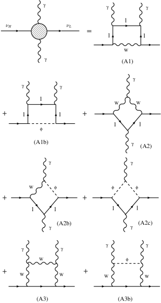
Figure 3: Electroweak one-loop Feynman diagrams for $\nu_{H}\to\nu_{L}\gamma\gamma$ in the ’t Hooft-Feynman gauge contributing to nondiagonal $\nu$–$e$ scattering on Fig. 2(b). Diagram (A2b) stands also for its counterpart diagram with $\phi$ and $W$ exchanged. There are some additional diagrams which do not contribute to the total $\nu_{L}\nu_{H}ee$ amplitude, as discussed in text.

The respective insertions enumerated on Fig. 3 build up the two-loop radiative amplitude

$$\mathcal{A}_{\text{rad}}^{\text{2L}}=\frac{G_{F}}{4\sqrt{2}}\frac{9}{4}\frac{\alpha^{2}}{\pi^{2}}\sum_{\alpha=\mu,\tau}\lambda_{\alpha}A_{(\alpha,e)}\bar{u}(p)\gamma^{\mu}(1-\gamma_{5})u(P)\>\bar{u}(k_{-})\gamma_{\mu}\gamma_{5}v(k_{+})\;,$$ (11)

which modifies the axial-vector form factor $f_{A}$. Note that potentially large logarithms of the type $\ln M_{W}^{2}/m_{l}^{2}$ get suppressed by the GIM mechanism.

The net result

$$f_{A}=\sum_{\alpha=\mu,\tau}\lambda_{\alpha}(1+\frac{9\alpha^{2}}{16\pi^{2}}A_{(\alpha,e)})\;,\\$$ (12)

is expressed in terms of the GIM-like combinations $A_{(\mu,e)}$ and $A_{(\tau,e)}$, displayed in Table 1.

Table 1: Contributions $A1,\ldots,A3b$ from Fig. 3 leading to the pertinent GIM-like loop-diagram factors $A_{(\tau,e)}$ and $A_{(\mu,e)}$.

      Diagram       $A_{(\tau,e)}$       $A_{(\mu,e)}$       A1       $21.4$       $14.0$       A1b       $-0.002$       $\sim 0$       A2       $0.0007$       $\sim 0$       A2b       $0.12$       $0.0007$       A2c       $0.009$       $\sim 0$       A3       $0.4$       $0.0001$       A3b       $0.03$       $\sim 0$       Total       $21.6$       $14.0$

Since the dominant contribution comes from the (A1) diagram in Fig. 3, one can rely on the simple leading-log analytical form of these functions ($A_{(\alpha,e)}\propto f_{\alpha}^{\text{2L}}$) in correspondence to the analytical expressions deduced previously [14, 13]. In close analogy to the one-loop radiative correction in (8) and (9), our two-loop radiative correction reads

$$f_{A} = \sum_{\alpha=\mu,\tau}\lambda_{\alpha}(1+f^{\text{2L}}_{\alpha})\;,$$ (13)

$$f^{\text{2L}}_{\alpha} = \frac{3}{4}\frac{\alpha^{2}}{\pi^{2}}\ln\frac{m_{\alpha}^{2}}{m_{e}^{2}}\;.$$ (14)

The dominant $\tau$-loop ($\alpha=\tau$) corrections to the referent tree-loop amplitude, given by expressions (9) and (14), are numerically

$$f^{\text{1L}}_{\tau}\simeq 6.3\times 10^{-3}\;,\quad f^{\text{2L}}_{\tau}\simeq 6.6\times 10^{-5}\;.$$ (15)

In order to estimate $f_{V}$ and $f_{A}$, one has to include also the PMNS-matrix prefactors, for which we now have the first strong experimental hints.

3 Conclusion

The existing neutrino experiments enable quite accurate global fits on the PMNS matrix elements. Unanticipated outcome of these experiments are large mixings. Let us, for definiteness, refer to the result of an earlier analysis by Fukugita and Tanimoto [15], based on the solar (SNO [2]) and atmospheric (SuperKamiokande [1]) neutrino data. Their solution shows a “democratic” mixing, very different from the “hierarchical” one experienced in the quark sector. The least known matrix element has been constrained here by the CHOOZ reactor experiment ($|U_{e3}|<0.16$).

Let us stress that for sufficiently heavy neutrino ($\nu_{H}$), such as the one allowed by the existing direct experimental mass limit of $\sim$18 MeV for $\nu_{\tau}$, the diagrams in Fig. 2 could give rise to the $\nu_{H}(P)\to\nu_{L}(p)e^{+}(k_{+})e^{-}(k_{-})$ decay. This decay was originally considered in [16], used for constraining the $|U_{e3}|$ PMNS matrix element in [17], and reconsidered later in [12]. However, the recent measurements squeeze neutrinos to sub-eV mass eigenstates that exclude this decay, and leave us with the scattering variant studied here.

In the meantime, an additional possibility to constrain $|U_{e3}|$ came with the results of KamLAND experiment [18]. For example, it allows in Ref. [19] to deduce the bounds $0.04<|U_{e3}|<0.19$. This prediction came on account of assuming Fritzsch-type lepton mass matrices adopted earlier by the same authors [20]. The range of parameters allowed by the KamLAND, as given by [19]

$$U_{\text{PMNS}}=\left(\begin{array}[]{ccc}0.76-0.86&0.50-0.63&0.04-0.19\\ 0.27-0.48&0.63-0.72&0.60-0.71\\ 0.34-0.49&0.42-0.58&0.71-0.80\\ \end{array}\right)\>,$$ (16)

turns out to be quite narrow and is a subject of future tests in neutrino experiments. These values enable us to give a definite prediction for $f_{V,A}$, which can be compared with the corresponding NSI contributions in (3).

The present bounds for the relevant NSI parameters are quite modest [5]

$$|\epsilon^{eL}_{\tau e}|<0.4\;,\qquad|\epsilon^{eR}_{\tau e}|<0.7\;.$$ (17)

They compare to $f_{L,R}=(f_{V}\pm f_{A})/2$ combinations of form factors (8) and (13)

$$|f_{L}|<0.16\;,\qquad|f_{R}|<1.3\times 10^{-3}\;,$$ (18)

where the loop results in (15) are further modulated by the matrix elements from (16). Thereby, the leading contribution given by $f^{1L}_{\tau}$ in (15) is numerically further suppressed. Consequently, the “standard” radiative corrections encoded in (2) can be confused with the left-handed $\epsilon^{L}$-couplings in (3), whereas the radiative corrections are small enough to allow for the discovery of the right-handed non-standard neutrino interactions.

References

- [1] Super-Kamiokande, Y. Fukuda et al., Phys. Rev. Lett. 81, 1562 (1998), hep-ex/9807003.
- [2] SNO, Q. R. Ahmad et al., Phys. Rev. Lett. 87, 071301 (2001), nucl-ex/0106015.
- [3] P. Huber, T. Schwetz, and J. W. F. Valle, Phys. Rev. D66, 013006 (2002), hep-ph/0202048.
- [4] Z. Berezhiani and A. Rossi, Phys. Lett. B535, 207 (2002), hep-ph/0111137.
- [5] S. Davidson, C. Pena-Garay, N. Rius, and A. Santamaria, (2003), hep-ph/0302093.
- [6] S. L. Adler, Phys. Rev. 177, 2426 (1969).
- [7] L. Rosenberg, Phys. Rev. 129, 2786 (1963).
- [8] B. Pontecorvo, Sov. Phys. JETP 7, 172 (1958).
- [9] Z. Maki, M. Nakagawa, and S. Sakata, Prog. Theor. Phys. 28, 870 (1962).
- [10] J. O. Eeg, K. Kumerički, and I. Picek, Eur. Phys. J. C17, 163 (2000), hep-ph/0007183.
- [11] J. O. Eeg, K. Kumerički, and I. Picek, Fizika B (2001), hep-ph/0203055.
- [12] Q. Ho-Kim, B. Machet, and X. Y. Pham, Eur. Phys. J. C13, 117 (2000), hep-ph/9902442.
- [13] J. O. Eeg, K. Kumerički, and I. Picek, Eur. Phys. J. C1, 531 (1998), hep-ph/9605337.
- [14] M. B. Voloshin and E. P. Shabalin, Pisma Zh. Eksp. Teor. Fiz. 23, 123 (1976).
- [15] M. Fukugita and M. Tanimoto, Phys. Lett. B515, 30 (2001), hep-ph/0107082.
- [16] R. E. Shrock, Phys. Rev. D24, 1275 (1981).
- [17] C. Hagner et al., Phys. Rev. D52, 1343 (1995).
- [18] KamLAND, K. Eguchi et al., Phys. Rev. Lett. 90, 021802 (2003), hep-ex/0212021.
- [19] M. Fukugita, M. Tanimoto, and T. Yanagida, (2003), hep-ph/0303177.
- [20] M. Fukugita, M. Tanimoto, and T. Yanagida, Prog. Theor. Phys. 89, 263 (1993).