Soft lepton-flavor violation
in a multi-Higgs-doublet seesaw model

Abstract

We consider the Standard Model with an arbitrary number $n_{H}$ of Higgs doublets and enlarge the lepton sector by adding to each lepton family $\ell$ a right-handed neutrino singlet $\nu_{\ell R}$. We assume that all the Yukawa-coupling matrices are diagonal, but the Majorana mass matrix $M_{R}$ of the right-handed neutrino singlets is an arbitrary symmetric matrix, thereby introducing an explicit but soft violation of all lepton numbers. We investigate lepton-flavor-violating processes within this model. We pay particular attention to the large-$m_{R}$ behavior of the amplitudes for these processes, where $m_{R}$ is the order of magnitude of the matrix elements of $M_{R}$. While the amplitudes for processes like $\tau^{-}\to\mu^{-}\gamma$ and $Z\to\tau^{+}\mu^{-}$ drop as $1/m_{R}^{2}$ for arbitrary $n_{H}$, processes like $\tau^{-}\to\mu^{-}e^{+}e^{-}$ and $\mu^{-}\to e^{-}e^{+}e^{-}$ obey this power law only for $n_{H}=1$. For $n_{H}\geq 2$, on the contrary, those amplitudes do not fall off when $m_{R}$ increases, rather they converge towards constants. This “non-decoupling” of the right-handed scale occurs because of the sub-process $\ell^{-}\to{\ell^{\prime}}^{-}{S_{b}^{0}}^{\ast}$, where $S_{b}^{0}$ is a neutral scalar which subsequently decays to $e^{+}e^{-}$. That sub-process has a contribution from charged-scalar exchange which, for $n_{H}\geq 2$, does not decrease when $m_{R}$ tends to infinity. We also perform a general study of the non-decoupling and argue that, at the one-loop level, after performing the limit $m_{R}\to\infty$ and after removing the $\nu_{R}$ from the Lagrangian, our model becomes a normal multi-Higgs-doublet Standard Model with loop-suppressed flavor-changing Yukawa couplings. Finally, we show that in our model the branching ratios of all lepton-flavor-changing processes are several orders of magnitude smaller than present experimental limits, if one makes the usual assumptions about the mass scales in the seesaw mechanism.

I Introduction

Recent experimental evidence strongly suggests that neutrinos mix and are, therefore, massive [1, 2, 3, 4]. This raises the question of why are the neutrino masses so much smaller than the masses of charged fermions. A simple answer to this question is provided by the seesaw mechanism [5]. In a seesaw model there are two mass scales:

  

$m_{D}$, the scale of the Dirac mass terms linking the (known) left-handed neutrinos to (new) right-handed neutrinos;

  

$m_{R}$, the scale of the Majorana mass terms of the right-handed neutrinos.

When $m_{R}\gg m_{D}$ the mixing of the two types of neutrinos gets suppressed by $m_{D}/m_{R}$ and the left-handed neutrinos acquire Majorana masses of order $m_{D}^{2}/m_{R}$, hence much smaller than the Dirac mass terms. Now, $m_{R}\gg m_{D}$ is natural, since the Majorana mass terms of the right-handed neutrinos are gauge-invariant; therefore, they do not need to be of order of the Fermi scale $m_{F}$ of the spontaneous breaking of the electroweak symmetry.

In the context of the seesaw mechanism an interesting option consists in having lepton-flavor symmetries which are respected by the Dirac mass terms, but broken by the Majorana mass terms of the right-handed neutrinos [6, 7]. This option arises because the Dirac mass terms originate in Yukawa couplings of the leptons to scalar doublets, which are hard (dimension four), while the Majorana mass terms are soft (dimension three). Lepton-flavor breaking thus becomes soft and, in fact, an unsuppressed reflection at low energies of some physics at ultra-high energies. This attractive hypothesis has the advantage that it allows one to construct simple models which explain the apparent maximal mixing of atmospheric neutrinos, solar neutrinos, or both simultaneously [7].

Once it is accepted that lepton-flavor breaking is soft, there is nothing against introducing many scalar doublets with Yukawa couplings to the leptons, since lepton-flavor-changing neutral interactions are automatically absent at tree level from those couplings. The question then arises of knowing whether lepton-flavor-violating decays, which arise at loop level, are suppressed by some powers of $m_{D}/m_{R}$ or $m_{F}/m_{R}$, or not. Moreover, one would like to identify the effective field theory at low scale which corresponds to the limit $m_{R}\to\infty$.

In this paper we try and answer the questions above by computing the lepton-flavor-violating decay $\tau^{-}\to\mu^{-}e^{+}e^{-}$ in the context of a seesaw model with an arbitrary number of scalar doublets and with softly-broken lepton numbers. We take this tau decay as a concrete example for the study of general features of our model. Since we compute the full one-loop decay amplitude for $\tau^{-}\to\mu^{-}e^{+}e^{-}$, we simultaneously also have the amplitudes for $\tau^{-}\to\mu^{-}\gamma$, $Z\to\tau^{+}\mu^{-}$, and $S^{0}_{b}\to\tau^{+}\mu^{-}$ at our disposal. ($S^{0}_{b}$ denotes a physical neutral scalar.) Evidently, the changes from tau decays to muon decays can be performed trivially in our results. There are in the literature a number of analogous computations (see Refs. [8, 9, 10, 11, 12, 13] and citations therein), yet our work is different for the following reasons:

1. In previous works the seesaw mechanism is considered in the context of the Standard Model, i.e. with only one Higgs doublet. There are then no physical charged scalars, and the neutral scalar—the Higgs particle—has been neglected because its Yukawa couplings are suppressed by the smallness of the charged-lepton masses. In the present work we consider charged scalars in the loops, and also neutral scalars $S_{b}^{0}$ in the process

   $$\tau^{-}\to\mu^{-}{S_{b}^{0}}^{\ast}\to\mu^{-}e^{+}e^{-}\,.$$ (1)

2. In previous works all external momenta have been set to zero. In this paper we give exact expressions for non-zero external momenta. Since the masses of the light neutrinos are much smaller than the masses of the charged leptons, it does not seem justified to treat the former exactly while neglecting the latter.

3. We study how the various contributions to the decay amplitude behave as functions of $m_{R}$. We demonstrate that the contributions previously computed are proportional to $1/m_{R}^{2}$, and thus negligible for sufficiently high $m_{R}$, while on the other hand some contributions to the process (1) remain unsuppressed.

In order to perform our computation in the context of a general multi-scalar-doublet model, we had to extend the formalism previously developed for the scalar particles in that model [14]. This formalism is presented in detail in Appendix A; it may be useful for other computations in that general model. We also took a close look at the one-loop renormalization of flavor-changing interactions; we show in Appendix B that the fermion wave-function renormalization, including fermion mixing, does not introduce any contributions to flavor-changing decays beyond those given by diagrams with flavor-changing self-energies in the external fermion legs [15].

This paper is organized as follows. In Section II we discuss the leptonic couplings and the necessary formulas concerning the seesaw mechanism. Section III treats some notation for the process $\tau^{-}\to\mu^{-}e^{+}e^{-}$, our example decay. Section IV deals with the orders of magnitude in our model and Section V introduces conventions and sub-processes for the example decay. Sections VI, VII, VIII, and IX describe, respectively, the photon, $Z$, neutral-scalar, and box-diagram sub-processes of $\tau^{-}\to\mu^{-}e^{+}e^{-}$. In Section X we discuss the limit of infinite right-handed scale. Section XI presents decay rates for the example decay and for other flavor-changing decays whose amplitudes have been implicitly calculated in Sections VI–VIII. The conclusions are found in Section XII.

II The leptonic couplings

A General seesaw framework

We consider an extension of the standard model with three families and three right-handed neutrinos. We label the latter with family lepton numbers: $\nu_{eR}$, $\nu_{\mu R}$, and $\nu_{\tau R}$. At the moment we do not assume conservation of the family lepton numbers, thus this labelling has no physical content. The Yukawa Lagrangian of the leptons is

$${\mathcal{L}}_{\mathrm{Y}}=-\sum_{k=1}^{n_{H}}\,\sum_{\ell,\ell^{\prime}=e,\mu,\tau}\left[\left(\begin{array}[]{cc}\varphi_{k}^{-},&{\varphi_{k}^{0}}^{\ast}\end{array}\right)\bar{\ell}_{R}\left(\Gamma_{k}\right)_{\ell\ell^{\prime}}+\left(\begin{array}[]{cc}\varphi_{k}^{0},&-\varphi_{k}^{+}\end{array}\right)\bar{\nu}_{\ell R}\left(\Delta_{k}\right)_{\ell\ell^{\prime}}\right]\left(\begin{array}[]{c}\nu_{\ell^{\prime}L}\\ \ell_{L}^{\prime}\end{array}\right)+\mathrm{H.c.}$$ (2)

The mass matrix of the charged leptons $M_{\ell}$ and the Dirac neutrino mass matrix $M_{D}$ are

$$M_{\ell}=\frac{1}{\sqrt{2}}\,\sum_{k}v_{k}^{\ast}\Gamma_{k}\quad\mathrm{and}\quad M_{D}=\frac{1}{\sqrt{2}}\,\sum_{k}v_{k}\Delta_{k}\,,$$ (3)

respectively. Without loss of generality, we assume $M_{\ell}$ to be diagonal with real and positive diagonal elements: $M_{\ell}=\mathrm{diag}\left(m_{e},m_{\mu},m_{\tau}\right)$. The mass terms for the neutrinos are

$$-\bar{\nu}_{R}M_{D}\nu_{L}-\frac{1}{2}\,\bar{\nu}_{R}CM_{R}\bar{\nu}_{R}^{T}+\mathrm{H.c.}\,,$$ (4)

where $C$ is the charge-conjugation matrix and $M_{R}$ is non-singular and symmetric.

The left- and right-handed neutrinos are written as linear superpositions of six physical Majorana neutrino fields $\chi_{i}$:

$$\nu_{\ell L}=\sum_{i}\left(U_{L}\right)_{\ell i}\gamma_{L}\chi_{i}\quad\mathrm{and}\quad\nu_{\ell R}=\sum_{i}\left(U_{R}\right)_{\ell i}\gamma_{R}\chi_{i}\,,$$ (5)

where $\gamma_{L}=\left(1-\gamma_{5}\right)/2$ and $\gamma_{R}=\left(1+\gamma_{5}\right)/2$ are the projectors of chirality. The fields $\chi_{i}$ satisfy $\chi_{i}=C\bar{\chi}_{i}^{T}$. The matrix

$${\mathcal{U}}=\left(\begin{array}[]{c}U_{L}\\ U_{R}^{\ast}\end{array}\right)$$ (6)

is $6\times 6$ unitary; therefore,

$$U_{L}U_{L}^{\dagger} = 1_{3\times 3}\,,$$ (7)

$$U_{R}U_{R}^{\dagger} = 1_{3\times 3}\,,$$ (8)

$$U_{L}U_{R}^{T} = 0_{3\times 3}\,,$$ (9)

and

$$U_{L}^{\dagger}U_{L}+U_{R}^{T}U_{R}^{\ast}=1_{6\times 6}\,.$$ (10)

${\mathcal{U}}$ is defined in such a way that

$${\mathcal{U}}^{T}\left(\begin{array}[]{cc}0&M_{D}^{T}\\ M_{D}&M_{R}\end{array}\right){\mathcal{U}}=\hat{m}=\mathrm{diag}\left(m_{1},m_{2},\ldots,m_{6}\right),$$ (11)

with real and non-negative $m_{i}$. Therefore,

$$U_{L}^{\ast}\hat{m}U_{L}^{\dagger} = 0_{3\times 3}\,,$$ (12)

$$U_{R}\hat{m}U_{L}^{\dagger} = M_{D}\,,$$ (13)

$$U_{R}\hat{m}U_{R}^{T} = M_{R}\,.$$ (14)

The charged-current Lagrangian is

$${\mathcal{L}}_{\mathrm{cc}}=\frac{g}{\sqrt{2}}\,\sum_{\ell,i}\left[W_{\mu}^{-}\left(U_{L}\right)_{\ell i}\bar{\ell}\gamma^{\mu}\gamma_{L}\chi_{i}+W_{\mu}^{+}\left(U_{L}^{\dagger}\right)_{i\ell}\bar{\chi}_{i}\gamma^{\mu}\gamma_{L}\ell\right].$$ (15)

The interaction of the $Z$ boson with the leptons is given by

$${\mathcal{L}}_{\mathrm{nc}} = \frac{g}{4c_{w}}\,Z_{\mu}\sum_{i,j}\bar{\chi}_{i}\gamma^{\mu}\left[\gamma_{L}\left(U_{L}^{\dagger}U_{L}\right)_{ij}-\gamma_{R}\left(U_{L}^{T}U_{L}^{\ast}\right)_{ij}\right]\chi_{j}$$ (17)

$$+\frac{g}{c_{w}}Z_{\mu}\sum_{\ell}\bar{\ell}\gamma^{\mu}\left(s_{w}^{2}-\frac{1}{2}\gamma_{L}\right)\ell\,.$$

When extracting the vertex from Eq. (17) one must multiply by a factor 2, since the neutrinos are Majorana fields.

The Yukawa couplings of the charged scalars $S_{a}^{\pm}$ to the leptons are written in the following general notation:

$${\mathcal{L}}_{\mathrm{Y}}\left(S^{\pm}\right)=\sum_{a,i,\ell}\left\{S_{a}^{-}\bar{\ell}\left[\left(R_{a}\right)_{\ell i}\gamma_{R}-\left(L_{a}\right)_{\ell i}\gamma_{L}\right]\chi_{i}+S_{a}^{+}\bar{\chi}_{i}\left[\left(R_{a}^{\dagger}\right)_{i\ell}\gamma_{L}-\left(L_{a}^{\dagger}\right)_{i\ell}\gamma_{R}\right]\ell\right\}.$$ (18)

The notation for the scalar sector, and the precise meaning of the $n_{H}$-vectors $a$, are explained in Appendix A 1. One has

$$R_{a}=\Delta_{a}^{\dagger}U_{R}\,, \mathrm{with} \Delta_{a}=\sum_{k}a_{k}\Delta_{k}\,,$$ (19)

$$L_{a}=\Gamma_{a}U_{L}\,, \mathrm{with} \Gamma_{a}=\sum_{k}a_{k}^{\ast}\Gamma_{k}\,.$$ (20)

Similarly, the Yukawa couplings of the neutral scalars $S^{0}_{b}$ (see again Appendix A 1) to the leptons are written

$${\mathcal{L}}_{\mathrm{Y}}\left(S^{0}\right) = -\frac{1}{\sqrt{2}}\,\sum_{b}S^{0}_{b}\left\{\sum_{i,j}\bar{\chi}_{i}\left[\left(F_{b}\right)_{ij}\gamma_{L}+\left(F_{b}^{\dagger}\right)_{ij}\gamma_{R}\right]\chi_{j}\right.$$ (22)

$$\left.+\sum_{\ell,\ell^{\prime}}\bar{\ell}\left[\left(\Gamma_{b}\right)_{\ell\ell^{\prime}}\gamma_{L}+\left(\Gamma_{b}^{\dagger}\right)_{\ell\ell^{\prime}}\gamma_{R}\right]\ell^{\prime}\right\},$$

with $\Gamma_{b}=\sum_{k}b_{k}^{\ast}\Gamma_{k}$. The matrices $F_{b}$ are symmetric:

$$F_{b}=\frac{1}{2}\left(U_{R}^{\dagger}\Delta_{b}U_{L}+U_{L}^{T}\Delta_{b}^{T}U_{R}^{\ast}\right),\quad\mathrm{with}\quad\Delta_{b}=\sum_{k}b_{k}\Delta_{k}\,.$$ (23)

When extracting the Feynman rule for the vertex with the neutrinos from Eq. (22), one should multiply by a factor 2, since the $\chi_{i}$ are self-conjugate fields.

In the case of the charged Goldstone bosons $G^{\pm}=S^{\pm}_{a_{W}}$ one has (see Appendix A.3) $\left(a_{W}\right)_{k}=gv_{k}/\left(2m_{W}\right)$. Therefore,

$$\Delta_{a_{W}} = \frac{g}{\sqrt{2}m_{W}}\,M_{D}\,,$$ (24)

$$\Gamma_{a_{W}} = \frac{g}{\sqrt{2}m_{W}}\,M_{\ell}\,,$$ (25)

and

$$R_{a_{W}} = \frac{g}{\sqrt{2}m_{W}}\,U_{L}\hat{m}\,,$$ (27)

$$L_{a_{W}} = \frac{g}{\sqrt{2}m_{W}}\,M_{\ell}U_{L}\,.$$ (28)

B Our model

We assume that the Yukawa-coupling matrices $\Gamma_{k}$ and $\Delta_{k}$ are simultaneously diagonal [7]. Therefore, the matrices $\Gamma_{a}$, $\Delta_{a}$, $\Gamma_{b}$, and $\Delta_{b}$ are all diagonal. The neutrino Dirac mass matrix $M_{D}$ is also diagonal, hence

$$U_{L}\hat{m}U_{R}^{\dagger}=M_{D}^{\dagger}\quad\mathrm{and}\quad U_{L}\hat{m}^{2}U_{L}^{\dagger}=M_{D}^{\dagger}M_{D}\quad\mathrm{are\ diagonal}.$$ (29)

Now the labelling of the neutrino fields according to family lepton numbers acquires a well-defined meaning.

Diagonal Yukawa-coupling matrices are achieved by assuming invariance of the Yukawa Lagrangian under $U(1)_{L_{\alpha}}$ ($\alpha=e,\mu,\tau$), the groups associated with conservation of the lepton number $L_{\alpha}$ for each lepton family. Since the gauge part of the Standard-Model Lagrangian is invariant under these $U(1)$ symmetries anyway, and since the scalar doublets do not transform under these $U(1)$ groups, the only place where these lepton-number symmetries are violated is the Majorana mass term of the right-handed singlets in Eq. (4). Since the mass term is an operator of dimension three, this violation is soft [7]. Hence, the one-loop amplitudes for lepton-flavor-violating processes must be finite.

III Notation for the process

The flavor-changing decay that we want to study is

$$\tau^{-}\left(p_{1}\right)\rightarrow\mu^{-}\left(p_{2}\right)e^{+}\left(p_{3}\right)e^{-}\left(p_{4}\right).$$ (30)

Clearly,

$$p_{1}^{2} = m_{\tau}^{2}\,,$$ (31)

$$p_{2}^{2} = m_{\mu}^{2}\,,$$ (32)

$$p_{3}^{2}=p_{4}^{2} = m_{e}^{2}\,.$$ (33)

We denote

$$\begin{array}[]{rcccl}q^{\alpha}&=&p_{1}^{\alpha}-p_{2}^{\alpha}&=&p_{3}^{\alpha}+p_{4}^{\alpha}\,,\\ r^{\alpha}&=&p_{1}^{\alpha}-p_{4}^{\alpha}&=&p_{2}^{\alpha}+p_{3}^{\alpha}\,,\end{array}$$ (34)

and

$$p_{+}^{\alpha}=\frac{p_{1}^{\alpha}+p_{2}^{\alpha}}{2}\,.$$ (35)

Then,

$$\begin{array}[]{rcccl}4m_{e}^{2}&\leq&q^{2}&\leq&\left(m_{\tau}-m_{\mu}\right)^{2}\,,\\ \left(m_{\mu}+m_{e}\right)^{2}&\leq&r^{2}&\leq&\left(m_{\tau}-m_{e}\right)^{2}\,.\end{array}$$ (36)

The amplitude $M$ for the process of Eq. (30) involves the Dirac spinors $\bar{u}_{\mu}=\bar{u}_{\mu}\left(p_{2}\right)$, $u_{\tau}=u_{\tau}\left(p_{1}\right)$, $\bar{u}_{e}=\bar{u}_{e}\left(p_{4}\right)$, and $v_{e}=v_{e}\left(p_{3}\right)$. These spinors satisfy

$$\bar{u}_{\mu}\!\!\not\!p_{2} = m_{\mu}\bar{u}_{\mu}\,,$$ (37)

$$\!\!\not\!p_{1}u_{\tau} = m_{\tau}u_{\tau}\,,$$ (38)

$$\bar{u}_{e}\!\!\not\!p_{4} = m_{e}\bar{u}_{e}\,,$$ (39)

$$\!\!\not\!p_{3}v_{e} = -m_{e}v_{e}\,.$$ (40)

In our calculations we shall often need the the following product of elements of $U_{L}$:

$$x_{i}=\left(U_{L}\right)_{\mu i}\left(U_{L}^{\dagger}\right)_{i\tau}\,,\quad\mathrm{satisfying}\quad\sum_{i}x_{i}=0\,,$$ (41)

where the second relation is a consequence of unitarity—see Eq. (7). Furthermore, we shall make use of dimensional regularization, evaluating integrals in a space–time of dimension $d$. Therefore, we define

$$d=4-2\epsilon\quad\mathrm{and}\quad{\mathcal{D}}k=d^{d}k/(2\pi)^{d}\,,$$ (42)

where the latter expression is an abbreviation for integration over the momentum $k$. Eventually, we shall take the limit $\epsilon\to 0$. Then, in some integrals the divergent constant

$$\mathcal{K}=\epsilon^{-1}-\gamma+\ln(4\pi)$$ (43)

will appear ($\gamma$ is Euler’s constant). The reason why $\mathcal{K}$ always drops out when calculating the amplitude for the process (30) in our model will be discussed in detail.

IV Orders of magnitude

We assume that the matrix elements of $M_{D}$ are of order $m_{D}$ and the square roots of the eigenvalues of $M_{R}^{\dagger}M_{R}$ are of order $m_{R}$, with $m_{D}\ll m_{R}$. Then,

$$\begin{array}[]{lclcl}{\displaystyle m_{i}\sim\frac{m_{D}^{2}}{m_{R}}}&\mathrm{and}&{\displaystyle\left(U_{R}\right)_{\ell i}\sim\frac{m_{D}}{m_{R}}}&\mathrm{for}&i=1,2,3\,;\\[11.38109pt] m_{i}\sim m_{R}&\mathrm{and}&{\displaystyle\left(U_{L}\right)_{\ell i}\sim\frac{m_{D}}{m_{R}}}&\mathrm{for}&i=4,5,6\,.\end{array}$$ (44)

There is also the order of magnitude, which we may call $m_{\ell}$, of the charged-lepton masses. This may be taken as either $m_{\tau}\sim 2$ GeV, or $m_{\mu}\sim 10^{-1}$ GeV, or $m_{e}\sim 5\times 10^{-4}$ GeV. Because of Eqs. (36), $q^{2}\sim r^{2}\sim m_{\ell}^{2}$. For simplicity we shall identify $m_{\ell}$ with $m_{D}$.

Finally, there is the Fermi scale $m_{F}$, in between 10 GeV and 1 TeV. The $W$ mass $m_{W}$, the charged-scalar masses $m_{a}$, and the neutral-scalar masses $m_{b}$ are all taken to be of order $m_{F}$. The scalar-potential couplings $C_{aa^{\prime}b}$ in Eq. (A47) are also assumed to be of order $m_{F}$. The overall hierarchy of mass scales is thus $m_{D}\ll m_{F}\ll m_{R}$.

When we have information about the masses of the light neutrinos we can estimate the order of magnitude of $m_{R}$ via the seesaw relation [5] in the first line of Eq. (44). If we take the light-neutrino masses to be of the order of $\sqrt{\Delta m^{2}_{\mathrm{atm}}}\sim 0.05$ eV, where $\Delta m^{2}_{\mathrm{atm}}$ is the neutrino mass-squared difference relevant for atmospheric-neutrino oscillations [1], and if we assume that $m_{D}\sim m_{\mu}$ or $m_{\tau}$, then we obtain $m_{R}\sim 10^{8}\div 10^{11}$ GeV. Thus we might regard $m_{R}\sim 10^{10}$ GeV as a typical order of magnitude of the right-handed scale, keeping in mind however that $m_{R}$ might deviate several orders of magnitude from this value.

It is important to notice that, with the convention $m_{\ell}=m_{D}$, the matrices $R_{a_{W}}$ and $L_{a_{W}}$ in Eqs. (27) and (28), giving the Yukawa couplings of the charged Goldstone boson, are of the same orders of magnitude as the corresponding general matrices $R_{a}$ and $L_{a}$ in Eqs. (20) and (19), provided we make the assumption

$$\Gamma_{j}\,,\Delta_{j}\sim m_{D}/m_{F}\,;$$ (45)

this is a natural relation in view of $m_{\ell}=m_{D}$. This means that the factors $m_{D}^{2}/m_{R}^{2}$ suppressing some charged-Goldstone-boson contributions are exactly the same as those suppressing the corresponding, and more general, charged-scalar contributions.

In the result for the momentum integrals large logarithms, like for instance $\ln(m_{R}/m_{F})$, arise. We shall not take into account such logarithms in our estimates of orders of magnitude.

V Conventions and sub-processes

We shall compute the process (30) using the conventions and vertices given in Ref. [16]. In the $Z^{0}$–$G^{0}$ sector we use the unitary gauge, thus discarding $G^{0}$. On the contrary, in the $W^{\pm}$–$G^{\pm}$ sector we use Feynman gauge. This means that the propagator of $W^{\pm}$ is $-ig_{\rho\sigma}/(k^{2}-m_{W}^{2})$. The charged-Goldstone-boson contributions will usually be taken into account together with the general charged-scalar contributions; the sums over the charged scalars $S_{a}^{\pm}$ will not exclude the charged Goldstone boson $G^{\pm}=S_{a_{W}}^{\pm}$. We remind that, in Feynman gauge, $m_{a_{W}}=m_{W}$.

The process (30) may proceed via box diagrams or through one of the three following sub-processes. In the sub-process with amplitude $\bar{M}_{A}$ the initial lepton $\tau^{-}$ decays into the final lepton $\mu^{-}$ together with a virtual photon $A$ with momentum $q$; the photon later decays into the $e^{+}e^{-}$ pair in the final state. The corresponding amplitude may be written

$$\bar{M}_{A}=\frac{M_{A}^{\rho}}{q^{2}}\,e\,\bar{u}_{e}\gamma_{\rho}v_{e}\,,$$ (46)

where $e$ is the positron charge and $M_{A}^{\rho}$ is the amplitude for $\tau^{-}\left(p_{1}\right)\to\mu^{-}\left(p_{2}\right)\gamma\left(q\right)$, the $\tau^{-}$ and the $\mu^{-}$ being on mass shell while the photon is off mass shell. Current conservation, i.e. Eqs. (39) and (40), implies that one may discard all terms proportional to $q^{\rho}$ from $M_{A}^{\rho}$. The sub-process with amplitude $\bar{M}_{Z}$ is analogous to the previous one with the virtual photon substituted by a virtual $Z$ boson. Its amplitude may be written

$$\bar{M}_{Z}=\frac{M_{Z}^{\rho}}{q^{2}-m_{Z}^{2}}\left(g_{\rho\theta}-\frac{q_{\rho}q_{\theta}}{m_{Z}^{2}}\right)\frac{g}{c_{w}}\,\bar{u}_{e}\gamma^{\theta}\left(s_{w}^{2}-\frac{\gamma_{L}}{2}\right)v_{e}\,.$$ (47)

Finally, there is the sub-process with amplitude $\bar{M}_{b}$, in which the $\tau^{-}$ decays into $\mu^{-}$ together with an off-shell neutral scalar $S^{0}_{b}$ with momentum $q$. The corresponding amplitude is

$$\bar{M}_{b}=\frac{M_{b}}{\sqrt{2}\left(q^{2}-m_{b}^{2}\right)}\,\bar{u}_{e}\left[\left(\Gamma_{b}\right)_{ee}\gamma_{L}+\left(\Gamma_{b}^{\dagger}\right)_{ee}\gamma_{R}\right]v_{e}\,.$$ (48)

One must sum $\bar{M}_{b}$ over all physical neutral scalars $b\neq b_{Z}$.

Besides these three sub-processes, there are also box diagrams, which are all finite, to be considered in Section IX.

No one-loop diagram with a neutral scalar $S_{b}^{0}$ in the loop can contribute to the process (30).

The infinities in the amplitude for the process (30) cancel for the following reasons:

1. Conservation of the electromagnetic current;

2. unitarity of the diagonalization matrix $\mathcal{U}$;

3. flavor-diagonal Yukawa-coupling matrices.

Item A is independent both of our model and of the seesaw mechanism, and applies to the photon sub-process. Concerning item B, the relations (7) and (9) are relevant, the first one in the form of Eq. (41). Only item C is directly connected with our model and, clearly, it plays a role only in charged-scalar exchange. More generally, items B and C are responsible for the cancellation of all terms independent of the neutrino masses $m_{i}$.

VI $\tau^{-}\to\mu^{-}A^{\ast}$

A Computation

Let us work out $M_{A}^{\rho}$ in detail. First consider the transition $\tau^{-}(p)\to\mu^{-}(p)$, effected either by $W^{\pm}$ exchange or by charged-scalar exchange. Call the corresponding amplitude $-i\Sigma(p)$. Then, there are the following two contributions to $M_{A}^{\rho}$:

$$M_{A1}^{\rho} = -e\bar{u}_{\mu}\gamma^{\rho}\,\frac{\ \!\!\not\!p_{1}+m_{\mu}}{m_{\tau}^{2}-m_{\mu}^{2}}\left[-i\Sigma\left(p_{1}\right)\right]u_{\tau}\,,$$ (49)

$$M_{A2}^{\rho} = -e\bar{u}_{\mu}\left[-i\Sigma\left(p_{2}\right)\right]\frac{\ \!\!\not\!p_{2}+m_{\tau}}{m_{\mu}^{2}-m_{\tau}^{2}}\,\gamma^{\rho}u_{\tau}\,.$$ (50)

We obtain for $\Sigma(p)$

$$-i\Sigma(p)=\int\!{\mathcal{D}}k\,\sum_{i}\frac{1}{D_{i}}\left[\frac{g^{2}x_{i}}{2}\,\frac{\left(d-2\right)\!\!\not\!k\gamma_{L}}{\left(k-p\right)^{2}-m_{W}^{2}}+\sum_{a}\frac{X_{ai}}{\left(k-p\right)-m_{a}^{2}}\right],$$ (51)

where

$$X_{ai} = \left(R_{a}\right)_{\mu i}\left(R_{a}^{\dagger}\right)_{i\tau}\,\!\!\not\!k\gamma_{L}+\left(L_{a}\right)_{\mu i}\left(L_{a}^{\dagger}\right)_{i\tau}\,\!\!\not\!k\gamma_{R}$$ (53)

$$-m_{i}\left(L_{a}\right)_{\mu i}\left(R_{a}^{\dagger}\right)_{i\tau}\gamma_{L}-m_{i}\left(R_{a}\right)_{\mu i}\left(L_{a}^{\dagger}\right)_{i\tau}\gamma_{R}\,.$$

The first term in the right-hand-side of Eq. (51) is the $W^{\pm}$-exchange contribution. The second term automatically includes, in the sum over $a$, the contribution of the charged Goldstone boson—which is obtained by setting $m_{a_{W}}=m_{W}$ and by using Eqs. (27) and (28) for the matrices $R_{a_{W}}$ and $L_{a_{W}}$.

There is one more contribution to $M_{A}^{\rho}$, namely from diagrams in which the photon attaches either to the $W^{\pm}$ or to the charged scalar in the loop. There is no $W^{\pm}S_{a}^{\mp}\gamma$ vertex except in the case $S_{a}^{\mp}=G^{\mp}$; also—see Appendix A 4—the vertex $W^{\pm}G^{\mp}\gamma$ has a factor $m_{W}$ which cancels the denominator $m_{W}^{-1}$ in the Yukawa coupling of $G^{\mp}$. One obtains the amplitude

$$M_{A3}^{\rho} = e\bar{u}_{\mu}\int\!{\mathcal{D}}k\,\sum_{i}\frac{1}{D_{i}}\left\{\frac{g^{2}x_{i}}{D_{1W}D_{2W}}\,\left[\left(d-2\right)\left(k-p_{+}\right)^{\rho}\!\!\not\!k\gamma_{L}-4k\cdot p_{+}\gamma^{\rho}\gamma_{L}+4p_{+}^{\rho}\!\!\not\!k\gamma_{L}\right.\right.$$ (55)

$$\left.\left.+m_{\tau}\left(\gamma^{\rho}\!\!\not\!k-\!\!\not\!k\gamma^{\rho}\right)\gamma_{R}+m_{\mu}\left(\,\!\!\not\!k\gamma^{\rho}-\gamma^{\rho}\!\!\not\!k\right)\gamma_{L}\right]+\sum_{a}\frac{2\left(k-p_{+}\right)^{\rho}X_{ai}}{D_{1a}D_{2a}}\right\}u_{\tau}\,.$$

We have used the shorthands

$$D_{\iota W}=\left(k-p_{\iota}\right)^{2}-m_{W}^{2}\quad\mathrm{and}\quad D_{\iota a}=\left(k-p_{\iota}\right)^{2}-m_{a}^{2}\,,\quad\mathrm{for}\quad\iota=1,2\,.$$ (56)

The sum over $a$ in Eq. (55) includes the contribution of the vertex $G^{+}G^{-}\gamma$. The other terms in the right-hand-side of that equation are the contributions from the vertex $W^{+}W^{-}\gamma$ and from the vertices $W^{\pm}G^{\mp}\gamma$.

Thus, $M_{A}^{\rho}=M_{A1}^{\rho}+M_{A2}^{\rho}+M_{A3}^{\rho}$.

One writes the Feynman integrals symbolically:

$$\int\!{\mathcal{D}}k\,\frac{1}{D_{i}D_{1W}}=a_{1}^{i}\,,\quad\int\!{\mathcal{D}}k\,\frac{k^{\theta}}{D_{i}D_{1W}}=b_{1}^{i}p_{1}^{\theta}\,;$$ (57)

$$\int\!{\mathcal{D}}k\,\frac{1}{D_{i}D_{2W}}=a_{2}^{i}\,,\quad\int\!{\mathcal{D}}k\,\frac{k^{\theta}}{D_{i}D_{2W}}=b_{2}^{i}p_{2}^{\theta}\,;$$ (58)

$$\begin{array}[]{l}{\displaystyle\int\!{\mathcal{D}}k\,\frac{1}{D_{i}D_{1W}D_{2W}}=a_{3}^{i}\,,\quad\int\!{\mathcal{D}}k\,\frac{k^{\theta}}{D_{i}D_{1W}D_{2W}}=c_{1}^{i}p_{1}^{\theta}+c_{2}^{i}p_{2}^{\theta}\,,}\\[14.22636pt] {\displaystyle\int\!{\mathcal{D}}k\,\frac{k^{\theta}k^{\psi}}{D_{i}D_{1W}D_{2W}}=d_{1}^{i}p_{1}^{\theta}p_{1}^{\psi}+d_{2}^{i}p_{2}^{\theta}p_{2}^{\psi}+f^{i}\left(p_{1}^{\theta}p_{2}^{\psi}+p_{2}^{\theta}p_{1}^{\psi}\right)+u^{i}g^{\theta\psi}.}\end{array}$$ (59)

In $a_{1}^{i},\ldots,u^{i}$, the index $i$ indicates the dependence on $m_{i}^{2}$. The coefficients $u^{i}$, $a_{1}^{i}$, $a_{2}^{i}$, $b_{1}^{i}$, and $b_{2}^{i}$ diverge when $d\to 4$, while all other coefficients are finite. However, the following relations hold:

$$a_{1}^{i}-a_{2}^{i} = q^{2}\left(c_{1}^{i}-c_{2}^{i}\right)+\left(m_{\tau}^{2}-m_{\mu}^{2}\right)k_{3}^{i}\,,$$ (60)

$$b_{1}^{i}-b_{2}^{i} = q^{2}\left(d_{1}^{i}-d_{2}^{i}\right)+\left(m_{\tau}^{2}-m_{\mu}^{2}\right)\left(k_{1}^{i}+k_{2}^{i}\right),$$ (61)

$$m_{\tau}^{2}b_{1}^{i}-m_{\mu}^{2}b_{2}^{i} = q^{2}\left(m_{\tau}^{2}d_{1}^{i}-m_{\mu}^{2}d_{2}^{i}\right)+\left(m_{\tau}^{2}-m_{\mu}^{2}\right)\left(2u^{i}-q^{2}f^{i}+m_{\tau}^{2}k_{1}^{i}+m_{\mu}^{2}k_{2}^{i}\right),$$ (62)

where

$$k_{1}^{i} = d_{1}^{i}+f^{i}-c_{1}^{i}\,,$$ (64)

$$k_{2}^{i} = d_{2}^{i}+f^{i}-c_{2}^{i}\,,$$ (65)

$$k_{3}^{i} = c_{1}^{i}+c_{2}^{i}-a_{3}^{i}\,.$$ (66)

One may write relations similar to Eqs. (57)–(66) for the integrals which have $D_{\iota a}$ instead of $D_{\iota W}$ (for $\iota=1,2$), then we use the notation $a_{1}^{i,a},\ldots,u^{i,a}$ in order to indicate the dependences on $m_{i}^{2}$ and on $m_{a}^{2}$.

Using Eqs. (60)–(LABEL:b1b2) one finds that $M^{\rho}_{A}$ is finite and that, moreover, it respects gauge invariance, i.e. $q_{\rho}M^{\rho}_{A}=0$:

$$M^{\rho}_{A} = e\sum_{i}\bar{u}_{\mu}\left\{i\sigma^{\rho\lambda}q_{\lambda}\left(\alpha_{Li}\,\gamma_{L}+\alpha_{Ri}\,\gamma_{R}\right)\right.$$ (69)

$$+\beta_{Li}\left[q^{\rho}\gamma_{L}-\frac{q^{2}}{m_{\tau}^{2}-m_{\mu}^{2}}\,\gamma^{\rho}\left(m_{\mu}\gamma_{L}+m_{\tau}\gamma_{R}\right)\right]$$

$$\left.+\beta_{Ri}\left[q^{\rho}\gamma_{R}-\frac{q^{2}}{m_{\tau}^{2}-m_{\mu}^{2}}\,\gamma^{\rho}\left(m_{\mu}\gamma_{R}+m_{\tau}\gamma_{L}\right)\right]\right\}u_{\tau}\,.$$

One obtains (for $d=4$)

$$\alpha_{Li} = g^{2}x_{i}m_{\mu}\left(k_{2}^{i}+c_{1}^{i}+c_{2}^{i}\right)$$ (71)

$$+\sum_{a}\left[m_{\mu}\left(R_{a}\right)_{\mu i}\left(R_{a}^{\dagger}\right)_{i\tau}k_{2}^{i,a}+m_{\tau}\left(L_{a}\right)_{\mu i}\left(L_{a}^{\dagger}\right)_{i\tau}k_{1}^{i,a}-m_{i}\left(L_{a}\right)_{\mu i}\left(R_{a}^{\dagger}\right)_{i\tau}k_{3}^{i,a}\right],$$

$$\alpha_{Ri} = g^{2}x_{i}m_{\tau}\left(k_{1}^{i}+c_{1}^{i}+c_{2}^{i}\right)$$ (74)

$$+\sum_{a}\left[m_{\tau}\left(R_{a}\right)_{\mu i}\left(R_{a}^{\dagger}\right)_{i\tau}k_{1}^{i,a}+m_{\mu}\left(L_{a}\right)_{\mu i}\left(L_{a}^{\dagger}\right)_{i\tau}k_{2}^{i,a}-m_{i}\left(R_{a}\right)_{\mu i}\left(L_{a}^{\dagger}\right)_{i\tau}k_{3}^{i,a}\right],$$

$$\beta_{Li} = g^{2}x_{i}m_{\mu}\left(k_{5}^{i}+c_{1}^{i}+c_{2}^{i}\right)$$ (77)

$$+\sum_{a}\left[m_{\mu}\left(R_{a}\right)_{\mu i}\left(R_{a}^{\dagger}\right)_{i\tau}k_{5}^{i,a}-m_{\tau}\left(L_{a}\right)_{\mu i}\left(L_{a}^{\dagger}\right)_{i\tau}k_{4}^{i,a}+m_{i}\left(L_{a}\right)_{\mu i}\left(R_{a}^{\dagger}\right)_{i\tau}\Delta c^{i,a}\right],$$

$$\beta_{Ri} = -g^{2}x_{i}m_{\tau}\left(k_{4}^{i}+c_{1}^{i}+c_{2}^{i}\right)$$ (80)

$$+\sum_{a}\left[-m_{\tau}\left(R_{a}\right)_{\mu i}\left(R_{a}^{\dagger}\right)_{i\tau}k_{4}^{i,a}+m_{\mu}\left(L_{a}\right)_{\mu i}\left(L_{a}^{\dagger}\right)_{i\tau}k_{5}^{i,a}+m_{i}\left(R_{a}\right)_{\mu i}\left(L_{a}^{\dagger}\right)_{i\tau}\Delta c^{i,a}\right],$$

where

$$k_{4}^{i} = f^{i}-d_{1}^{i}\,,$$ (82)

$$k_{5}^{i} = f^{i}-d_{2}^{i}\,,$$ (83)

and similarly for the coefficients $k_{4}^{i,a}$ and $k_{5}^{i,a}$. Also, $\Delta c^{i,a}=c_{2}^{i,a}-c_{1}^{i,a}$.

B Order of magnitude

Integrating over the momentum $k$ one finds, from Eqs. (59),

$$\left(a_{3}^{i},c_{1}^{i},c_{2}^{i},d_{1}^{i},d_{2}^{i},f^{i}\right)=\frac{-i}{16\pi^{2}}\,\int_{0}^{1}\!dx\int_{0}^{1-x}\!dy\,\frac{1}{\Delta_{i}^{W}}\left(1,y,x,y^{2},x^{2},xy\right),$$ (84)

where

$$\Delta_{i}^{W}=\left(x+y\right)m_{W}^{2}+\left(1-x-y\right)\left(m_{i}^{2}-xm_{\mu}^{2}-ym_{\tau}^{2}\right)-xyq^{2}\,.$$ (85)

Let us denote by $g^{i}$ a generic coefficient $a_{3}^{i}$, $c_{1,2}^{i}$, $d_{1,2}^{i}$, or $f^{i}$, and similarly $g^{i,a}$ for $a_{3}^{i,a}$, etc. Clearly, $g^{i}$ is a function of $m_{i}^{2}$, with $g^{i}\sim m_{F}^{-2}$ for $i=1,2,3$ and $g^{i}\sim m_{R}^{-2}$ for $i=4,5,6$. Moreover, for $i=1,2,3$, $g^{i}$ is independent of $m_{i}$ up to corrections of order $m_{i}^{2}/m_{W}^{2}\sim m_{D}^{4}/\left(m_{R}^{2}m_{F}^{2}\right)$. The same holds for the $g^{i,a}$, of course.

Considering Eqs. (69)–(LABEL:betaRi) in detail, we see that $M_{A}^{\rho}$ involves terms of five types:

1. $g^{2}m_{\ell}^{2}\sum_{i}x_{i}g^{i}$;

2. $m_{\ell}^{2}\sum_{i}\left(R_{a}\right)_{\mu i}\left(R_{a}^{\dagger}\right)_{i\tau}g^{i,a}$;

3. $m_{\ell}^{2}\sum_{i}\left(L_{a}\right)_{\mu i}\left(L_{a}^{\dagger}\right)_{i\tau}g^{i,a}$;

4. $m_{\ell}\sum_{i}m_{i}\left(R_{a}\right)_{\mu i}\left(L_{a}^{\dagger}\right)_{i\tau}g^{i,a}$;

5. $m_{\ell}\sum_{i}m_{i}\left(L_{a}\right)_{\mu i}\left(R_{a}^{\dagger}\right)_{i\tau}g^{i,a}$.

We remind the reader that we set $m_{\ell}\sim m_{D}$. Also, from Eqs. (19) and (20), we see that $L_{a}$ is $U_{L}$ and $R_{a}$ is $U_{R}$ except for diagonal Yukawa-coupling matrices.

Terms of types 1 and 3 are similar. They are proportional to $(U_{L})_{\mu i}(U_{L}^{\dagger})_{i\tau}$, which is of order 1 for $i=1,2,3$ and of order $m_{D}^{2}/m_{R}^{2}$ for $i=4,5,6$. As we have seen, $g^{i}\sim m_{F}^{-2}$ is almost independent of $i$ for $i=1,2,3$. One may therefore use

$$\sum_{i=1}^{3}x_{i}=-\sum_{i=4}^{6}x_{i}\sim\frac{m_{D}^{2}}{m_{R}^{2}}$$ (86)

to estimate $m_{\ell}^{2}\sum_{i=1}^{3}x_{i}g^{i}$ to be of order $m_{D}^{4}/\left(m_{R}^{2}m_{F}^{2}\right)$. For $i=4,5,6$ one has $g^{i}\sim m_{R}^{-2}$ and $x_{i}\sim m_{D}^{2}/m_{R}^{2}$, hence terms of type 1 or 3 are of order $m_{D}^{4}/m_{R}^{4}$.

Terms of type 2 are proportional to $(U_{R})_{\mu i}(U_{R}^{\dagger})_{i\tau}$. Therefore, for $i=1,2,3$ they are of order $m_{D}^{4}/\left(m_{R}^{2}m_{F}^{2}\right)$ and for $i=4,5,6$ they are of order $m_{D}^{2}/m_{R}^{2}$.

Finally, terms of types 4 and 5 always include a suppression $m_{D}/m_{R}$ from the mixing matrices $U_{L}$ and $U_{R}$. Taking into account also $m_{\ell}$, $m_{i}$, and $g^{i,a}$, those terms are of order $m_{D}^{4}/\left(m_{R}^{2}m_{F}^{2}\right)$ for $i=1,2,3$, or $m_{D}^{2}/m_{R}^{2}$ for $i=4,5,6$.

In summary, we find that the amplitude for the vertex $\tau^{-}\to\mu^{-}A^{\ast}$ is suppressed by $m_{D}^{2}/m_{R}^{2}$. With $m_{D}\sim 1$ GeV and $m_{R}\sim 10^{10}$ GeV one has a suppression factor $10^{-20}$ in the amplitude of $\tau\to\mu\gamma$. Note that terms of type 2–5 contain a product of two Yukawa coupling constants. If we are more specific and assume the relation (45) for the Yukawa couplings, then there is a suppression factor of order $m_{D}^{4}/(m_{R}^{2}m_{F}^{2})$ for all of them and, in addition, a $(16\pi^{2})^{-1}$ from the loop integration. Terms of type 1, on the other hand, have an extra factor $g^{2}$.

VII $\tau^{-}\to\mu^{-}Z^{\ast}$

A Graphs in which the $Z$ attaches to charged particles

The vertex $\tau^{-}\to\mu^{-}Z^{\ast}$ has three contributions $M_{Z1}^{\rho}$, $M_{Z2}^{\rho}$, and $M_{Z3}^{\rho}$ analogous to the corresponding contributions to $\tau^{-}\to\mu^{-}A^{\ast}$. Comparing them one easily concludes that

$$M_{Z1}^{\rho}+M_{Z2}^{\rho}+M_{Z3}^{\rho}=\frac{g\left(s_{w}^{2}-c_{w}^{2}\right)}{2ec_{w}}\,M_{A}^{\rho}+\frac{g}{2c_{w}}\,T^{\rho}\,,$$ (87)

with

$$T^{\rho} = -\bar{u}_{\mu}\left\{\gamma^{\rho}\gamma_{R}\,\frac{\ \!\!\not\!p_{1}+m_{\mu}}{m_{\tau}^{2}-m_{\mu}^{2}}\left[-i\Sigma\left(p_{1}\right)\right]+\left[-i\Sigma\left(p_{2}\right)\right]\frac{\ \!\!\not\!p_{2}+m_{\tau}}{m_{\mu}^{2}-m_{\tau}^{2}}\,\gamma^{\rho}\gamma_{R}\right\}u_{\tau}$$ (90)

$$+\bar{u}_{\mu}\int\!{\mathcal{D}}k\,\sum_{i}\frac{g^{2}x_{i}}{D_{i}D_{1W}D_{2W}}\left[\left(2-d\right)\left(k-p_{+}\right)^{\rho}\!\!\not\!k\gamma_{L}+4k\cdot p_{+}\gamma^{\rho}\gamma_{L}-4p_{+}^{\rho}\!\!\not\!k\gamma_{L}\right.$$

$$\left.+m_{\tau}\!\!\not\!k\gamma^{\rho}\gamma_{R}+m_{\mu}\gamma^{\rho}\!\!\not\!k\gamma_{L}-2m_{i}^{2}\gamma^{\rho}\gamma_{L}\right]u_{\tau}\,.$$

We compute $T^{\rho}$ by using the same method as in Eqs. (57)–(83), arriving at the result

$$T^{\rho} = -\left(\bar{u}_{\mu}\gamma_{R}u_{\tau}\right)\sum_{i}g^{2}x_{i}m_{\tau}\left[2p_{+}^{\rho}\left(k_{1}^{i}+c_{1}^{i}\right)-q^{\rho}\left(k_{4}^{i}+c_{1}^{i}\right)\right]$$ (93)

$$-\left(\bar{u}_{\mu}\gamma_{L}u_{\tau}\right)\sum_{i}g^{2}x_{i}m_{\mu}\left[2p_{+}^{\rho}\left(k_{2}^{i}+c_{2}^{i}\right)+q^{\rho}\left(k_{5}^{i}+c_{2}^{i}\right)\right]$$

$$+\bar{u}_{\mu}\gamma^{\rho}\sum_{i}\left(L_{i}\gamma_{L}+R_{i}\gamma_{R}\right)u_{\tau}\,,$$

where

$$L_{i} = g^{2}x_{i}\left[\left(2-d\right)u^{i}-2m_{i}^{2}a_{3}^{i}+\left(2m_{\tau}^{2}+m_{\mu}^{2}-q^{2}\right)c_{1}^{i}+\left(m_{\tau}^{2}+2m_{\mu}^{2}-q^{2}\right)c_{2}^{i}\right],$$ (94)

$$R_{i} = g^{2}x_{i}m_{\mu}m_{\tau}\left[c_{1}^{i}+c_{2}^{i}-k_{1}^{i}-k_{2}^{i}+\frac{q^{2}}{m_{\tau}^{2}-m_{\mu}^{2}}\left(d_{2}^{i}-d_{1}^{i}\right)\right]$$ (98)

$$+\sum_{a}\left\{\left(R_{a}\right)_{\mu i}\left(R_{a}^{\dagger}\right)_{i\tau}m_{\mu}m_{\tau}\left[-k_{1}^{i,a}-k_{2}^{i,a}+\frac{q^{2}}{m_{\tau}^{2}-m_{\mu}^{2}}\left(d_{2}^{i,a}-d_{1}^{i,a}\right)\right]\right.$$

$$+\left(L_{a}\right)_{\mu i}\left(L_{a}^{\dagger}\right)_{i\tau}\!\left[-2u^{i,a}+q^{2}f^{i,a}-m_{\tau}^{2}k_{1}^{i,a}-m_{\mu}^{2}k_{2}^{i,a}+\frac{q^{2}}{m_{\tau}^{2}-m_{\mu}^{2}}\left(m_{\mu}^{2}d_{2}^{i,a}-m_{\tau}^{2}d_{1}^{i,a}\right)\!\right]$$

$$\left.+m_{i}\left[m_{\tau}\left(L_{a}\right)_{\mu i}\left(R_{a}^{\dagger}\right)_{i\tau}+m_{\mu}\left(R_{a}\right)_{\mu i}\left(L_{a}^{\dagger}\right)_{i\tau}\right]\left[k_{3}^{i,a}+\frac{q^{2}}{m_{\tau}^{2}-m_{\mu}^{2}}\left(c_{1}^{i,a}-c_{2}^{i,a}\right)\right]\right\}.$$

Let us consider the order of magnitude of $T^{\rho}$. We realize at a glance that most of its terms are of one of the five types already considered in Subsection VI B. In $L_{i}$ there is a term $x_{i}m_{i}^{2}a_{3}^{i}$, which is of order $m_{D}^{2}/m_{R}^{2}$ for $i=4,5,6$ and additionally suppressed for $i=1,2,3$. The main originality of the $T^{\rho}$ is, however, the presence of a term with $u^{i}$ in $L_{i}$ and with $u^{i,a}$ in $R_{i}$. Computing the divergent coefficient $u^{i}$ one finds

$$u^{i}=\frac{i}{32\pi^{2}}\,\int_{0}^{1}\!dx\int_{0}^{1-x}\!dy\,\left(\mathcal{K}-\ln{\Delta_{i}^{W}}\right),$$ (99)

where the infinite constant $\mathcal{K}$ is defined in Eq. (43). Now, $\mathcal{K}$ is independent of $i$ and cancels out when one sums over $i$. This happens in the case of $u^{i}$ because $\sum_{i}x_{i}=0$, and in the case of $u^{i,a}$ because $(L_{a}L_{a}^{\dagger})_{\mu\tau}=(\Gamma_{a}\Gamma_{a}^{\dagger})_{\mu\tau}=0$; the last relation holds because the matrices $\Gamma_{a}$ are diagonal, which is a specific property of our model. In $u^{i}$, Eq. (99), and also in $u^{i,a}$ one may, therefore, discard the divergence. We may also substitute $\ln{\Delta_{i}^{W}}$ by the logarithm of the dimensionless quantity $\Delta_{i}^{W}/\Delta_{1}^{W}$. This logarithm is large for $i=4,5,6$ while for $i=1,2,3$ it is of order $m_{D}^{4}/\left(m_{R}^{2}m_{F}^{2}\right)$. The order of magnitude of $\sum_{i}x_{i}u^{i}$ and $\sum_{i}(L_{a})_{\mu i}(L_{a}^{\dagger})_{i\tau}u^{i,a}$ is, therefore, $m_{D}^{2}/m_{R}^{2}$.

In summary, $\sum_{\iota=1}^{3}M_{Z\iota}^{\rho}$ is suppressed by $m_{D}^{2}/m_{R}^{2}$, even in the presence of charged scalars.

B Graphs in which the $Z$ attaches to neutrinos

There are also contributions to $M_{Z}^{\rho}$ in which the $Z$ boson attaches to the neutrino line, thereby changing the neutrino eigenstate from $\chi_{j}$ to $\chi_{i}$. The corresponding vertex is given by Eq. (17), with an extra factor 2 because of the self-conjugated character of the neutrinos. One obtains a contribution $M^{\rho}_{Z4}$ to $M_{Z}^{\rho}$, and $M_{Z}^{\rho}=\sum_{\iota=1}^{4}M_{Z\iota}^{\rho}$. Let us define

$$D_{ij}^{W}=xm_{i}^{2}+ym_{j}^{2}+\left(1-x-y\right)\left(m_{W}^{2}-xm_{\mu}^{2}-ym_{\tau}^{2}\right)-xyq^{2}\,,$$ (100)

and similarly $D_{ij}^{a}$, which is identical to $D_{ij}^{W}$ with $m_{W}$ substituted by $m_{a}$. We then find

$$M^{\rho}_{Z4} = \frac{-ig^{3}}{32\pi^{2}c_{w}}\,\sum_{i,j}\left(U_{L}\right)_{\mu i}\left(U_{L}^{\dagger}\right)_{j\tau}\,\int_{0}^{1}\!dx\,\int_{0}^{1-x}\!dy\ \bar{u}_{\mu}\left[\frac{\xi_{1}^{\rho}\left(U_{L}^{T}U_{L}^{\ast}\right)_{ij}+\xi_{2}^{\rho}\left(U_{L}^{\dagger}U_{L}\right)_{ij}}{D^{W}_{ij}}\right.$$ (104)

$$\left.+\left(U_{L}^{\dagger}U_{L}\right)_{ij}\gamma^{\rho}\gamma_{L}\left(\ln{D_{ij}^{W}}-\mathcal{K}+2\right)\right]u_{\tau}$$

$$+\frac{-ig}{32\pi^{2}c_{w}}\,\sum_{i,j}\sum_{a}\int_{0}^{1}\!dx\,\int_{0}^{1-x}\!dy\ \bar{u}_{\mu}\left\{\frac{\xi_{3}^{\rho}}{D_{ij}^{a}}+\gamma^{\rho}\left[\left(L_{a}\right)_{\mu i}\left(U_{L}^{\dagger}U_{L}\right)_{ij}\left(L_{a}^{\dagger}\right)_{j\tau}\gamma_{R}\right.\right.$$

$$\left.\left.-\left(R_{a}\right)_{\mu i}\left(U_{L}^{T}U_{L}^{\ast}\right)_{ij}\left(R_{a}^{\dagger}\right)_{j\tau}\gamma_{L}\right]\left(\ln{D^{a}_{ij}}-\mathcal{K}+1\right)\right\}u_{\tau}\,,$$

with

$$\xi_{1}^{\rho}=m_{i}m_{j}\gamma^{\rho}\gamma_{L}\,,$$ (105)

$$\xi_{2}^{\rho} = \left[2p_{1}\cdot p_{2}\left(1-x\right)\left(1-y\right)+m_{\mu}^{2}x\left(x-1\right)+m_{\tau}^{2}y\left(y-1\right)\right]\gamma^{\rho}\gamma_{L}$$ (108)

$$+m_{\mu}m_{\tau}\left(1-x-y\right)\gamma^{\rho}\gamma_{R}$$

$$+2m_{\mu}\left(1-x\right)\left[p_{2}^{\rho}x-p_{1}^{\rho}\left(1-y\right)\right]\gamma_{L}+2m_{\tau}\left(1-y\right)\left[p_{1}^{\rho}y-p_{2}^{\rho}\left(1-x\right)\right]\gamma_{R}\,,$$

$$\xi_{3}^{\rho} = m_{i}m_{j}\gamma^{\rho}\left[\left(L_{a}\right)_{\mu i}\left(U_{L}^{T}U_{L}^{\ast}\right)_{ij}\left(L_{a}^{\dagger}\right)_{j\tau}\gamma_{R}-\left(R_{a}\right)_{\mu i}\left(U_{L}^{\dagger}U_{L}\right)_{ij}\left(R_{a}^{\dagger}\right)_{j\tau}\gamma_{L}\right]$$ (120)

$$+m_{i}m_{\tau}\left(1-y\right)\gamma^{\rho}\left[\left(R_{a}\right)_{\mu i}\left(U_{L}^{\dagger}U_{L}\right)_{ij}\left(L_{a}^{\dagger}\right)_{j\tau}\gamma_{L}-\left(L_{a}\right)_{\mu i}\left(U_{L}^{T}U_{L}^{\ast}\right)_{ij}\left(R_{a}^{\dagger}\right)_{j\tau}\gamma_{R}\right]$$

$$+m_{i}x\left(m_{\mu}\gamma^{\rho}-2p_{2}^{\rho}\right)\left[\left(R_{a}\right)_{\mu i}\left(U_{L}^{\dagger}U_{L}\right)_{ij}\left(L_{a}^{\dagger}\right)_{j\tau}\gamma_{R}-\left(L_{a}\right)_{\mu i}\left(U_{L}^{T}U_{L}^{\ast}\right)_{ij}\left(R_{a}^{\dagger}\right)_{j\tau}\gamma_{L}\right]$$

$$+m_{j}m_{\mu}\left(1-x\right)\gamma^{\rho}\left[\left(L_{a}\right)_{\mu i}\left(U_{L}^{\dagger}U_{L}\right)_{ij}\left(R_{a}^{\dagger}\right)_{j\tau}\gamma_{L}-\left(R_{a}\right)_{\mu i}\left(U_{L}^{T}U_{L}^{\ast}\right)_{ij}\left(L_{a}^{\dagger}\right)_{j\tau}\gamma_{R}\right]$$

$$+m_{j}y\left[\left(L_{a}\right)_{\mu i}\left(U_{L}^{\dagger}U_{L}\right)_{ij}\left(R_{a}^{\dagger}\right)_{j\tau}\gamma_{L}-\left(R_{a}\right)_{\mu i}\left(U_{L}^{T}U_{L}^{\ast}\right)_{ij}\left(L_{a}^{\dagger}\right)_{j\tau}\gamma_{R}\right]\left(m_{\tau}\gamma^{\rho}-2p_{1}^{\rho}\right)$$

$$+m_{\mu}m_{\tau}\left(1-x-y\right)\gamma^{\rho}\left[\left(R_{a}\right)_{\mu i}\left(U_{L}^{T}U_{L}^{\ast}\right)_{ij}\left(R_{a}^{\dagger}\right)_{j\tau}\gamma_{R}-\left(L_{a}\right)_{\mu i}\left(U_{L}^{\dagger}U_{L}\right)_{ij}\left(L_{a}^{\dagger}\right)_{j\tau}\gamma_{L}\right]$$

$$+m_{\mu}x\left(1-x\right)$$

$$\times\left(m_{\mu}\gamma^{\rho}-2p_{2}^{\rho}\right)\left[\left(R_{a}\right)_{\mu i}\left(U_{L}^{T}U_{L}^{\ast}\right)_{ij}\left(R_{a}^{\dagger}\right)_{j\tau}\gamma_{L}-\left(L_{a}\right)_{\mu i}\left(U_{L}^{\dagger}U_{L}\right)_{ij}\left(L_{a}^{\dagger}\right)_{j\tau}\gamma_{R}\right]$$

$$+m_{\tau}y\left(1-y\right)$$

$$\times\left[\left(R_{a}\right)_{\mu i}\left(U_{L}^{T}U_{L}^{\ast}\right)_{ij}\left(R_{a}^{\dagger}\right)_{j\tau}\gamma_{R}-\left(L_{a}\right)_{\mu i}\left(U_{L}^{\dagger}U_{L}\right)_{ij}\left(L_{a}^{\dagger}\right)_{j\tau}\gamma_{L}\right]\left(m_{\tau}\gamma^{\rho}-2p_{1}^{\rho}\right)$$

$$+xy\left[\left(R_{a}\right)_{\mu i}\left(U_{L}^{T}U_{L}^{\ast}\right)_{ij}\left(R_{a}^{\dagger}\right)_{j\tau}\left(2m_{\mu}p_{1}^{\rho}\gamma_{L}+2m_{\tau}p_{2}^{\rho}\gamma_{R}-2p_{1}\cdot p_{2}\gamma^{\rho}\gamma_{L}\right)\right.$$

$$\left.-\left(L_{a}\right)_{\mu i}\left(U_{L}^{\dagger}U_{L}\right)_{ij}\left(L_{a}^{\dagger}\right)_{j\tau}\left(2m_{\mu}p_{1}^{\rho}\gamma_{R}+2m_{\tau}p_{2}^{\rho}\gamma_{L}-2p_{1}\cdot p_{2}\gamma^{\rho}\gamma_{R}\right)\right].$$

As before, $\mathcal{K}$ does not depend on $m_{i}$ and on $m_{j}$ and cancels out when one sums Eq. (104) over $i$ and over $j$. The cancellations occurs in the second line as a consequence of Eq. (7) and in the fourth line as a consequence of (9) and the form of $R_{a}$ in Eq. (19), which are properties of the general seesaw framework; in the case of the term $(L_{a})_{\mu i}(U_{L}^{\dagger}U_{L})_{ij}(L_{a}^{\dagger})_{j\tau}$, cancellation upon summation over $i$ and over $j$ also hinges upon the fact that the matrices $\Gamma_{a}$ are diagonal, which is a property of our specific model.

We are therefore free to subtract from $\ln{D^{W}_{ij}}$ in Eq. (104) its value when $i=j=1$, i.e. its value when both $\chi_{i}$ and $\chi_{j}$ are the lightest neutrino. We obtain $\ln{(D^{W}_{ij}/D^{W}_{11})}$, which is zero for $i=j=1$, of order $m_{D}^{4}/\left(m_{R}^{2}m_{F}^{2}\right)$ when $i\in\left\{1,2,3\right\}$ and $j\in\left\{2,3\right\}$ or vice-versa, and large otherwise. We similarly substitute $\ln{D^{a}_{ij}}$ by $\ln{(D^{a}_{ij}/D^{a}_{11})}$.

It is now possible to evaluate the order of magnitude of each contribution to $M_{Z4}^{\rho}$. After tedious yet straightforward consideration, we conclude that all terms are suppressed by, at least, $m_{D}^{2}/m_{R}^{2}$. In most cases this suppression applies term by term; in some exceptional cases one must sum the contributions over the light neutrinos and apply Eq. (86). This happens, for instance, with

$$\left(U_{L}\right)_{\mu i}\left(U_{L}^{\dagger}U_{L}\right)_{ij}\left(U_{L}^{\dagger}\right)_{j\tau}\int_{0}^{1}\!dx\,\int_{0}^{1-x}\!dy\ \frac{1}{D^{W}_{ij}}\,,$$ (121)

which is of order $m_{F}^{-2}$ for $i,j\in\left\{1,2,3\right\}$ but acquires a suppression $m_{D}^{2}/m_{R}^{2}$ when $i$ and $j$ are both summed over the light neutrinos.

In conclusion, the contributions to the decay (30) from both photon or $Z$ exchange are all suppressed by $m_{D}^{2}/m_{R}^{2}$, even in the presence of extra scalar doublets. This suppression also ensures that the simpler processes $\tau^{-}\to\mu^{-}\gamma$ and $Z\to\tau^{+}\mu^{-}$ are invisible in all feasible experiments. We next look to the contributions to the decay (30) from neutral-scalar exchange.

VIII $\tau^{-}\to\mu^{-}{S^{0}_{b}}^{*}$

A Self-energy graphs

Similarly to what happens with the couplings to the photon and $Z$ boson, there are two self-energy graphs for the coupling to the neutral scalar $S^{0}_{b}$:

$$M_{b1} = \frac{1}{\sqrt{2}}\,\bar{u}_{\mu}\left(\Gamma_{b}\gamma_{L}+\Gamma_{b}^{\dagger}\gamma_{R}\right)_{\mu\mu}\frac{\not\!p_{1}+m_{\mu}}{m_{\tau}^{2}-m_{\mu}^{2}}\left[-i\Sigma(p_{1})\right]u_{\tau}\,,$$ (122)

$$M_{b2} = \frac{1}{\sqrt{2}}\,\bar{u}_{\mu}\left[-i\Sigma(p_{2})\right]\frac{\not\!p_{2}+m_{\tau}}{m_{\mu}^{2}-m_{\tau}^{2}}\left(\Gamma_{b}\gamma_{L}+\Gamma_{b}^{\dagger}\gamma_{R}\right)_{\tau\tau}u_{\tau}\,.$$ (123)

The difference relative to the case of the gauge bosons lies in the fact that $S^{0}_{b}$ couples differently to the charged leptons $\tau$ and $\mu$—in the first case with the Yukawa coupling $\left(\Gamma_{b}\right)_{\tau\tau}$, in the second case with $\left(\Gamma_{b}\right)_{\mu\mu}$. As a consequence, it is not possible to use Eqs. (60)–(LABEL:b1b2) and we must compute $\Sigma(p)$ explicitly. Define

$$D_{i}^{W} = xm_{i}^{2}+\left(1-x\right)\left(m_{W}^{2}-xp^{2}\right),$$ (124)

$$D_{i}^{a} = xm_{i}^{2}+\left(1-x\right)\left(m_{a}^{2}-xp^{2}\right).$$ (125)

The relevant integrals are then

$$f_{i}^{a} = \int_{0}^{1}\!dx\,\ln{\frac{D_{i}^{a}}{D_{1}^{a}}}\,,$$ (126)

$$g_{i}^{a} = \int_{0}^{1}\!dx\left(1-x\right)\ln{\frac{D_{i}^{a}}{D_{1}^{a}}}\,,$$ (127)

together with $f_{i}^{W}$ and $g_{i}^{W}$ analogously defined. One has

$$-i\Sigma(p) = \frac{-i}{16\pi^{2}}\,\sum_{i}\,\left\{g^{2}x_{i}\,g_{i}^{W}\!\!\!\not\!p\gamma_{L}+\sum_{a}g_{i}^{a}\!\!\not\!p\left[\left(R_{a}\right)_{\mu i}\left(R_{a}^{\dagger}\right)_{i\tau}\gamma_{L}+\left(L_{a}\right)_{\mu i}\left(L_{a}^{\dagger}\right)_{i\tau}\gamma_{R}\right]\right.$$ (129)

$$\left.-\sum_{a}f_{i}^{a}m_{i}\left[\left(L_{a}\right)_{\mu i}\left(R_{a}^{\dagger}\right)_{i\tau}\gamma_{L}+\left(R_{a}\right)_{\mu i}\left(L_{a}^{\dagger}\right)_{i\tau}\gamma_{R}\right]\right\}.$$

As in the previous section, in the original definitions of $f_{i}^{a}$ and $g_{i}^{a}$ there should be a divergence $\mathcal{K}$ added to the logarithms. However, $\mathcal{K}$ is $i$-independent and yields a null contribution to $\Sigma(p)$ upon summation over $i$. This happens because of Eqs. (7) and (8) and because in our model the matrices $\Gamma_{a}$ and $\Delta_{a}$ are diagonal; in the second line of Eq. (129) we also need the first Eq. (29) for $(L_{a}\hat{m}R_{a}^{\dagger})_{\mu\tau}=(\Gamma_{a}U_{L}\hat{m}U_{R}^{\dagger}\Delta_{a})_{\mu\tau}=(\Gamma_{a}M_{D}^{\dagger}\Delta_{a})_{\mu\tau}=0$. In the definitions of $f_{i}^{a}$ and of $g_{i}^{a}$ we could, therefore, subtract from $\ln{D_{i}^{a}}$ its value for $i=1$, i.e. for the lightest neutrino; this subtraction corresponds to an $i$-independent subtraction from $f_{i}^{a}$ and from $g_{i}^{a}$ and, therefore, to a null contribution to $\Sigma(p)$.

It is clear from Eqs. (122) and (123) that the relevant $p^{2}$ in $\Sigma(p)$ is either $m_{\mu}^{2}$ or $m_{\tau}^{2}$. When $i=1,2,3$ one has $m_{i}^{2}\ll p^{2}\ll m_{a}^{2}$; when $i=4,5,6$ one has $p^{2}\ll m_{a}^{2}\ll m_{i}^{2}$. It is clear that, for $i=1,2,3$, the logarithm of $D_{i}^{a}/D_{1}^{a}$ is—neglecting $p^{2}\ll m_{a}^{2}$—approximately proportional to $\left(m_{i}^{2}-m_{1}^{2}\right)/m_{a}^{2}\sim m_{D}^{4}/\left(m_{R}^{2}m_{F}^{2}\right)$. The same happens with the logarithm of $D_{i}^{W}/D_{1}^{W}$. Therefore, the contributions of the light neutrinos to $\Sigma(p)$ are suppressed by $m_{D}^{4}/\left(m_{R}^{2}m_{F}^{2}\right)$. On the other hand, some contributions of the heavy neutrinos remain unsuppressed. For $i=4,5,6$ one has

$$f_{i}^{a} \approx \ln{\frac{m_{i}^{2}}{m_{a}^{2}}}\,,$$ (130)

$$g_{i}^{a} \approx \frac{1}{2}\left(\ln{\frac{m_{i}^{2}}{m_{a}^{2}}}-1\right)\,.$$ (131)

Matrix elements of $U_{L}$, as in $x_{i}$ and in $(L_{a})_{\mu i}(L_{a}^{\dagger})_{i\tau}$, suppress some of the contributions of the heavy neutrinos. Overall one obtains the unsuppressed part

$$\Sigma(p) \approx \frac{1}{16\pi^{2}}\,\sum_{i=4}^{6}\sum_{a}\ln{\frac{m_{i}^{2}}{m_{a}^{2}}}\left\{\frac{\,\,\!\!\not\!p\gamma_{L}}{2}\left(R_{a}\right)_{\mu i}\left(R_{a}^{\dagger}\right)_{i\tau}\right.$$ (133)

$$\left.-m_{i}\left[\left(L_{a}\right)_{\mu i}\left(R_{a}^{\dagger}\right)_{i\tau}\gamma_{L}+\left(R_{a}\right)_{\mu i}\left(L_{a}^{\dagger}\right)_{i\tau}\gamma_{R}\right]\right\}.$$

Note that the sum over $a$ includes a contribution from the charged Goldstone boson.

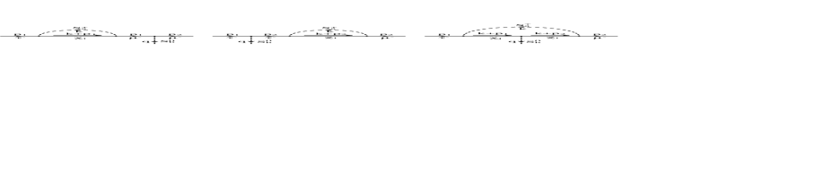
FIG. 1.: The three diagrams for $\tau^{-}\to\mu^{-}{S_{b}^{0}}^{*}$ which have parts unsuppressed by $m_{R}^{-1}$.

We conclude that some contributions of the heavy neutrinos to $M_{b1}$ and to $M_{b2}$ remain unsuppressed when $m_{R}\to\infty$. Let us compute those contributions in detail. Using

$$m_{i}\left(U_{L}\right)_{\ell i}=\left(M_{D}^{\ast}\right)_{\ell\ell}\left(U_{R}\right)_{\ell i}\,,$$ (134)

which is valid in our specific seesaw model for any $\ell$ and $i$, we rewrite Eq. (133) as

$$\Sigma(p) \approx \frac{1}{16\pi^{2}}\,\sum_{i=4}^{6}\left[\left(U_{R}\right)_{\mu i}\left(U_{R}^{\dagger}\right)_{i\tau}\ln{\frac{m_{i}^{2}}{\mu^{2}}}\right]\sum_{a}\left[\frac{\,\,\!\!\not\!p\gamma_{L}}{2}\left(\Delta_{a}^{\ast}\right)_{\mu\mu}\left(\Delta_{a}\right)_{\tau\tau}\right.$$ (136)

$$\left.-\left(\Gamma_{a}\right)_{\mu\mu}\left(M_{D}^{\ast}\right)_{\mu\mu}\left(\Delta_{a}\right)_{\tau\tau}\gamma_{L}-\left(\Delta_{a}^{\ast}\right)_{\mu\mu}\left(M_{D}\right)_{\tau\tau}\left(\Gamma_{a}^{\ast}\right)_{\tau\tau}\gamma_{R}\right]$$

$$= \frac{1}{16\pi^{2}}\,\sum_{i=4}^{6}\left[\left(U_{R}\right)_{\mu i}\left(U_{R}^{\dagger}\right)_{i\tau}\ln{\frac{m_{i}^{2}}{\mu^{2}}}\right]\sum_{k}\left[\frac{\,\,\!\!\not\!p\gamma_{L}}{2}\left(\Delta_{k}^{\ast}\right)_{\mu\mu}\left(\Delta_{k}\right)_{\tau\tau}\right.$$ (138)

$$\left.-\left(\Gamma_{k}\right)_{\mu\mu}\left(M_{D}^{\ast}\right)_{\mu\mu}\left(\Delta_{k}\right)_{\tau\tau}\gamma_{L}-\left(\Delta_{k}^{\ast}\right)_{\mu\mu}\left(M_{D}\right)_{\tau\tau}\left(\Gamma_{k}^{\ast}\right)_{\tau\tau}\gamma_{R}\right],$$

where $\mu$ is an arbitrary mass, inserted for dimensional reasons; the expression (138) is independent of it. Inserting this result into Eqs. (122) and (123), we obtain—see Fig. 1 for the relevant self-energy graphs—

$$M_{b1}+M_{b2}\approx{\displaystyle\frac{-i}{16\sqrt{2}\pi^{2}}\,\frac{\sum_{i=4}^{6}\left[\left(U_{R}\right)_{\mu i}\left(U_{R}^{\dagger}\right)_{i\tau}\ln\left(m_{i}^{2}/\mu^{2}\right)\right]}{m_{\tau}^{2}-m_{\mu}^{2}}}\,\bar{u}_{\mu}\left(A_{L}\gamma_{L}+A_{R}\gamma_{R}\right)u_{\tau}\,,$$ (139)

with

$$A_{L} = \left[m_{\tau}\left(\Gamma_{b}\right)_{\mu\mu}-m_{\mu}\left(\Gamma_{b}\right)_{\tau\tau}\right]\left[\frac{m_{\tau}}{2}\,\sum_{k}\left(\Delta_{k}^{\ast}\right)_{\mu\mu}\left(\Delta_{k}\right)_{\tau\tau}-\left(M_{D}\right)_{\tau\tau}\sum_{k}\left(\Delta_{k}^{\ast}\right)_{\mu\mu}\left(\Gamma_{k}^{\ast}\right)_{\tau\tau}\right]$$ (141)

$$+\left[m_{\tau}\left(\Gamma_{b}\right)_{\tau\tau}-m_{\mu}\left(\Gamma_{b}\right)_{\mu\mu}\right]\left(M_{D}^{\ast}\right)_{\mu\mu}\sum_{k}\left(\Gamma_{k}\right)_{\mu\mu}\left(\Delta_{k}\right)_{\tau\tau}\,,$$

$$A_{R} = \left[m_{\tau}\left(\Gamma_{b}^{\ast}\right)_{\mu\mu}-m_{\mu}\left(\Gamma_{b}^{\ast}\right)_{\tau\tau}\right]\left[\frac{m_{\mu}}{2}\,\sum_{k}\left(\Delta_{k}^{\ast}\right)_{\mu\mu}\left(\Delta_{k}\right)_{\tau\tau}-\left(M_{D}^{\ast}\right)_{\mu\mu}\sum_{k}\left(\Gamma_{k}\right)_{\mu\mu}\left(\Delta_{k}\right)_{\tau\tau}\right]$$ (143)

$$+\left[m_{\tau}\left(\Gamma_{b}^{\ast}\right)_{\tau\tau}-m_{\mu}\left(\Gamma_{b}^{\ast}\right)_{\mu\mu}\right]\left(M_{D}\right)_{\tau\tau}\sum_{k}\left(\Delta_{k}^{\ast}\right)_{\mu\mu}\left(\Gamma_{k}^{\ast}\right)_{\tau\tau}\,.$$

B Graphs in which $S^{0}_{b}$ couples to charged bosons

The necessary couplings are found in Appendices A 4 and A 5. Let us define

$$D_{i}^{aa^{\prime}}=xm_{a}^{2}+ym_{a^{\prime}}^{2}+\left(1-x-y\right)\left(m_{i}^{2}-xm_{\tau}^{2}-ym_{\mu}^{2}\right)-xyq^{2}\,.$$ (144)

Then, the graph in which $S^{0}_{b}$ couples to (incoming) $S_{a}^{-}$ and $S_{a^{\prime}}^{+}$ yields

$$M_{baa^{\prime}} = \frac{-i}{16\pi^{2}}\,\sum_{i}\sum_{a,a^{\prime}}C_{aa^{\prime}b}\,\int_{0}^{1}\!dx\,\int_{0}^{1-x}\!dy\ \frac{1}{D_{i}^{aa^{\prime}}}$$ (147)

$$\times\,\bar{u}_{\mu}\left[\left(R_{a^{\prime}}\right)_{\mu i}\left(R_{a}^{\dagger}\right)_{i\tau}\left(xm_{\tau}\gamma_{R}+ym_{\mu}\gamma_{L}\right)+\left(L_{a^{\prime}}\right)_{\mu i}\left(L_{a}^{\dagger}\right)_{i\tau}\left(xm_{\tau}\gamma_{L}+ym_{\mu}\gamma_{R}\right)\right.$$

$$\left.-m_{i}\left(R_{a^{\prime}}\right)_{\mu i}\left(L_{a}^{\dagger}\right)_{i\tau}\gamma_{R}-m_{i}\left(L_{a^{\prime}}\right)_{\mu i}\left(R_{a}^{\dagger}\right)_{i\tau}\gamma_{L}\right]u_{\tau}\,.$$

The cases in which either $S_{a}^{-}$, or $S_{a^{\prime}}^{+}$, or both, are charged Goldstone bosons, are implicitly covered through Eqs. (27), (28), and (A51), (A53). The graph in which $S^{0}_{b}$ couples to $W^{-}$ and $S_{a}^{+}$ gives

$$M_{bWa} = \frac{-ig^{2}}{32\sqrt{2}\pi^{2}}\,\sum_{i}\left(U_{L}^{\dagger}\right)_{i\tau}\sum_{a}b^{\dagger}a\,\int_{0}^{1}\!dx\,\int_{0}^{1-x}\!dy$$ (151)

$$\times\,\bar{u}_{\mu}\left\{\frac{\left(R_{a}\right)_{\mu i}m_{i}}{D_{i}^{Wa}}\left[\left(x+1\right)m_{\tau}\gamma_{R}+\left(y-2\right)m_{\mu}\gamma_{L}\right]\right.$$

$$-\frac{\left(L_{a}\right)_{\mu i}}{D_{i}^{Wa}}\left[\left(2x+y\right)m_{\mu}m_{\tau}\gamma_{R}+x\left(1+x\right)m_{\tau}^{2}\gamma_{L}\right.$$

$$\left.\left.+y\left(y-2\right)m_{\mu}^{2}\gamma_{L}+2x\left(y-2\right)p_{1}\cdot p_{2}\gamma_{L}\right]-2\left(L_{a}\right)_{\mu i}\gamma_{L}\,\ln{\frac{D_{i}^{Wa}}{D_{1}^{Wa}}}\right\}u_{\tau}\,.$$

Similarly, the graph in which $S^{0}_{b}$ couples to $S_{a}^{-}$ and $W^{+}$ contributes

$$M_{baW} = \frac{-ig^{2}}{32\sqrt{2}\pi^{2}}\,\sum_{i}\left(U_{L}\right)_{\mu i}\sum_{a}a^{\dagger}b\,\int_{0}^{1}\!dx\,\int_{0}^{1-x}\!dy$$ (155)

$$\times\,\bar{u}_{\mu}\left\{\frac{\left(R_{a}^{\dagger}\right)_{i\tau}m_{i}}{D_{i}^{aW}}\left[\left(y+1\right)m_{\mu}\gamma_{L}+\left(x-2\right)m_{\tau}\gamma_{R}\right]\right.$$

$$-\frac{\left(L_{a}^{\dagger}\right)_{i\tau}}{D_{i}^{aW}}\left[\left(2y+x\right)m_{\mu}m_{\tau}\gamma_{L}+x\left(x-2\right)m_{\tau}^{2}\gamma_{R}\right.$$

$$\left.\left.+y\left(1+y\right)m_{\mu}^{2}\gamma_{R}+2y\left(x-2\right)p_{1}\cdot p_{2}\gamma_{R}\right]-2\left(L_{a}^{\dagger}\right)_{i\tau}\gamma_{R}\,\ln{\frac{D_{i}^{aW}}{D_{1}^{aW}}}\right\}u_{\tau}\,.$$

Finally, there is a graph with the $S^{0}_{b}$ attaching to two $W^{\pm}$ bosons, yielding

$$M_{bWW}=\frac{-ig^{3}m_{W}}{16\pi^{2}}\,a_{W}^{\dagger}b\,\sum_{i}x_{i}\,\int_{0}^{1}\!dx\,\int_{0}^{1-x}\!dy\ \bar{u}_{\mu}\frac{xm_{\tau}\gamma_{R}+ym_{\mu}\gamma_{L}}{D_{i}^{WW}}\,u_{\tau}\,.$$ (156)

Any part of the integrals which does not depend on $m_{i}$ ends up, upon summation over $i$, giving a zero contribution to $M_{b}$. One may therefore subtract from each integral its value when $m_{i}=m_{1}$. In Eqs. (151) and (155) we have already performed that subtraction in the logarithmic terms. The infinities which occurred together with the logarithms in those expressions have been dropped using $(L_{a}U_{L}^{\dagger})_{\mu\tau}=(\Gamma_{a})_{\mu\tau}=0$ in Eq. (151) and the Hermitian-conjugate relation in Eq. (155). The amplitudes (147) and (156) have only finite integrals.

Consider for instance $M_{baa^{\prime}}$ in Eq. (147). The term with $R_{a^{\prime}}R_{a}^{\dagger}$ is proportional to $(U_{R})_{\mu i}(U_{R}^{\dagger})_{i\tau}$. For $i=1,2,3$ it is suppressed by $m_{D}^{2}/m_{R}^{2}$ from the matrix $U_{R}$; it is additionally suppressed by $C_{aa^{\prime}b}$ and the integral, giving together a factor $m_{D}/m_{F}$. For $i=4,5,6$ the suppression factor is $m_{F}m_{D}/m_{R}^{2}$.

The term with $L_{a^{\prime}}L_{a}^{\dagger}$ has $(U_{L})_{\mu i}(U_{L}^{\dagger})_{i\tau}$. For $i=1,2,3$ we neglect the neutrino masses $m_{i}$ in the integral and use Eq. (86) to obtain the same order of magnitude as for the term $R_{a^{\prime}}R_{a}^{\dagger}$. For $i=4,5,6$ we have suppressions $m_{D}^{2}/m_{R}^{2}$ from $U_{L}$ and $m_{F}m_{D}/m_{R}^{2}$ from the rest of the term.

The terms with $R_{a^{\prime}}L_{a}^{\dagger}$ and $L_{a^{\prime}}R_{a}^{\dagger}$ have suppressions $m_{D}/m_{R}$ from the mixing. For $i=1,2,3$ there is also $m_{i}$ and the integral, yielding together suppressions $m_{D}^{2}/\left(m_{R}m_{F}\right)$. For $i=4,5,6$ $m_{i}\sim m_{R}$ and the integral is of order $m_{R}^{-2}$, and we correspondingly obtain $m_{F}/m_{R}$ in addition to the mixing suppression.

In conclusion, all contributions to $M_{baa^{\prime}}$ are suppressed by, at least, $m_{F}m_{D}/m_{R}^{2}$. In the same way, one finds that $M_{bWa}$ and $M_{baW}$ are suppressed by $m_{D}^{2}/m_{R}^{2}$ while $M_{bWW}$ is suppressed by $m_{D}^{3}/\left(m_{R}^{2}m_{F}\right)$.

C Graphs in which $S^{0}_{b}$ couples to neutrinos

We remind the reader of the quantity $D_{ij}^{W}$ defined in Eq. (100), and of the analogous quantity $D_{ij}^{a}$. We find, for the contribution to $M_{b}$ in which $S^{0}_{b}$ couples to neutrinos, the result

$$M_{b4}=\frac{-i\sqrt{2}}{16\pi^{2}}\,\int_{0}^{1}\!dx\int_{0}^{1-x}\!dy\ \bar{u}_{\mu}\sum_{i,j}\left(\frac{Z_{ij}^{W}}{D_{ij}^{W}}+\sum_{a}\frac{Z_{ij}^{a}}{D_{ij}^{a}}-2\sum_{a}Z_{ij}^{\prime a}\ln{\frac{D_{ij}^{a}}{D_{11}^{a}}}\right)u_{\tau}\,.$$ (157)

Here,

$$Z_{ij}^{W} = g^{2}\left(U_{L}\right)_{\mu i}\left(U_{L}^{\dagger}\right)_{j\tau}\left[\left(1-x\right)m_{\mu}m_{j}\left(F_{b}^{\dagger}\right)_{ij}\gamma_{L}+\left(1-y\right)m_{i}m_{\tau}\left(F_{b}\right)_{ij}\gamma_{R}\right.$$ (159)

$$\left.-ym_{j}m_{\tau}\left(F_{b}^{\dagger}\right)_{ij}\gamma_{R}-xm_{\mu}m_{i}\left(F_{b}\right)_{ij}\gamma_{L}\right],$$

$$Z_{ij}^{a} = -m_{i}m_{j}\left[\left(R_{a}\right)_{\mu i}\left(F_{b}^{\dagger}\right)_{ij}\left(L_{a}^{\dagger}\right)_{j\tau}\gamma_{R}+\left(L_{a}\right)_{\mu i}\left(F_{b}\right)_{ij}\left(R_{a}^{\dagger}\right)_{j\tau}\gamma_{L}\right]$$ (167)

$$+m_{i}m_{\tau}\left(1-y\right)\left[\left(R_{a}\right)_{\mu i}\left(F_{b}^{\dagger}\right)_{ij}\left(R_{a}^{\dagger}\right)_{j\tau}\gamma_{R}+\left(L_{a}\right)_{\mu i}\left(F_{b}\right)_{ij}\left(L_{a}^{\dagger}\right)_{j\tau}\gamma_{L}\right]$$

$$-m_{i}m_{\mu}x\left[\left(R_{a}\right)_{\mu i}\left(F_{b}^{\dagger}\right)_{ij}\left(R_{a}^{\dagger}\right)_{j\tau}\gamma_{L}+\left(L_{a}\right)_{\mu i}\left(F_{b}\right)_{ij}\left(L_{a}^{\dagger}\right)_{j\tau}\gamma_{R}\right]$$

$$+m_{\mu}m_{j}\left(1-x\right)\left[\left(L_{a}\right)_{\mu i}\left(F_{b}^{\dagger}\right)_{ij}\left(L_{a}^{\dagger}\right)_{j\tau}\gamma_{R}+\left(R_{a}\right)_{\mu i}\left(F_{b}\right)_{ij}\left(R_{a}^{\dagger}\right)_{j\tau}\gamma_{L}\right]$$

$$-m_{\tau}m_{j}y\left[\left(L_{a}\right)_{\mu i}\left(F_{b}^{\dagger}\right)_{ij}\left(L_{a}^{\dagger}\right)_{j\tau}\gamma_{L}+\left(R_{a}\right)_{\mu i}\left(F_{b}\right)_{ij}\left(R_{a}^{\dagger}\right)_{j\tau}\gamma_{R}\right]$$

$$-m_{\mu}m_{\tau}\left(1-x-y\right)\left[\left(L_{a}\right)_{\mu i}\left(F_{b}^{\dagger}\right)_{ij}\left(R_{a}^{\dagger}\right)_{j\tau}\gamma_{R}+\left(R_{a}\right)_{\mu i}\left(F_{b}\right)_{ij}\left(L_{a}^{\dagger}\right)_{j\tau}\gamma_{L}\right]$$

$$+\left[x\left(1-x\right)m_{\mu}^{2}+y\left(1-y\right)m_{\tau}^{2}-xy\left(m_{\mu}^{2}+m_{\tau}^{2}-q^{2}\right)\right]$$

$$\times\left[\left(L_{a}\right)_{\mu i}\left(F_{b}^{\dagger}\right)_{ij}\left(R_{a}^{\dagger}\right)_{j\tau}\gamma_{L}+\left(R_{a}\right)_{\mu i}\left(F_{b}\right)_{ij}\left(L_{a}^{\dagger}\right)_{j\tau}\gamma_{R}\right],$$

and

$$Z_{ij}^{\prime a}=\left(L_{a}\right)_{\mu i}\left(F_{b}^{\dagger}\right)_{ij}\left(R_{a}^{\dagger}\right)_{j\tau}\gamma_{L}+\left(R_{a}\right)_{\mu i}\left(F_{b}\right)_{ij}\left(L_{a}^{\dagger}\right)_{j\tau}\gamma_{R}\,.$$ (168)

In Eq. (157) we have already dropped the infinity occurring together with the logarithm, because, using all the previous arguments for the cancellation of terms independent of $m_{i}$, we find $\sum_{i,j}Z_{ij}^{\prime a}=0$.

It is tedious but straightforward to check that all the terms in $Z_{ij}^{W}$ and in $Z_{ij}^{a}$ end up suppressed by $1/m_{R}^{2}$ or by higher powers of $m_{R}^{-2}$. The same does not happen, however, with the terms in $Z^{\prime a}_{ij}$ (which include a contribution from the charged Goldstone boson for $a=a_{W}$). Let us write the latter in more detail, using Eqs. (19), (20), (23), and the fact that the matrices $\Gamma_{a}$, $\Delta_{a}$, and $\Delta_{b}$ are diagonal:

$$2Z^{\prime a}_{ij} = \left(\Gamma_{a}\right)_{\mu\mu}\left(\Delta_{a}\right)_{\tau\tau}\left(U_{L}\right)_{\mu i}\left(U_{L}^{\dagger}\Delta_{b}^{\ast}U_{R}+U_{R}^{T}\Delta_{b}^{\ast}U_{L}^{\ast}\right)_{ij}\left(U_{R}^{\dagger}\right)_{j\tau}\gamma_{L}$$ (170)

$$+\left(\Delta_{a}^{\ast}\right)_{\mu\mu}\left(\Gamma_{a}^{\ast}\right)_{\tau\tau}\left(U_{R}\right)_{\mu i}\left(U_{R}^{\dagger}\Delta_{b}U_{L}+U_{L}^{T}\Delta_{b}U_{R}^{\ast}\right)_{ij}\left(U_{L}^{\dagger}\right)_{j\tau}\gamma_{R}\,.$$

Due to Eqs. (44), terms unsuppressed by $m_{D}/m_{R}$ may arise only from the first term in the right-hand-side of Eq. (170), when $i=1,2,3$ and $j=4,5,6$, and from the third term in the right-hand-side of Eq. (170), when $i=4,5,6$ and $j=1,2,3$. In the first case the integral of $\ln{D_{ij}^{a}}$ is practically $i$-independent, in the second case it is almost $j$-independent. One obtains the following contribution to $M_{b4}$, with the corresponding Feynman diagram depicted in Fig. 1:

$$M_{b4}^{a} \approx \frac{i}{16\sqrt{2}\pi^{2}}\sum_{i=4}^{6}\left[\left(U_{R}\right)_{\mu i}\left(U_{R}^{\dagger}\right)_{i\tau}\ln{\frac{m_{i}^{2}}{\mu^{2}}}\right]\bar{u}_{\mu}\left[\left(\Delta_{b}^{\ast}\right)_{\mu\mu}\sum_{k}\left(\Gamma_{k}\right)_{\mu\mu}\left(\Delta_{k}\right)_{\tau\tau}\gamma_{L}\right.$$ (172)

$$\left.+\left(\Delta_{b}\right)_{\tau\tau}\sum_{k}\left(\Delta_{k}^{\ast}\right)_{\mu\mu}\left(\Gamma_{k}^{\ast}\right)_{\tau\tau}\gamma_{R}\right]u_{\tau}\,.$$

This expression is independent of the arbitrary mass $\mu$. $M_{b4}$ is not fully suppressed by powers of $m_{R}$ since $M_{b4}^{a}$ becomes constant in the limit $m_{R}\to\infty$.

D Unsuppressed terms

We thus conclude that the vertex $\tau^{-}\to\mu^{-}{S_{b}^{0}}^{\ast}$ does not vanish in the limit $m_{R}\to\infty$. One has

$$M_{b}^{\infty} = \frac{i}{16\sqrt{2}\pi^{2}}\,\sum_{i=4}^{6}\left[\left(U_{R}\right)_{\mu i}\left(U_{R}^{\dagger}\right)_{i\tau}\ln{\frac{m_{i}^{2}}{\mu^{2}}}\right]$$ (175)

$$\times\bar{u}_{\mu}\left\{\left[\left(\Delta_{b}^{\ast}\right)_{\mu\mu}\sum_{k}\left(\Gamma_{k}\right)_{\mu\mu}\left(\Delta_{k}\right)_{\tau\tau}+\frac{A_{L}}{m_{\mu}^{2}-m_{\tau}^{2}}\right]\gamma_{L}\right.$$

$$\left.+\left[\left(\Delta_{b}\right)_{\tau\tau}\sum_{k}\left(\Delta_{k}^{\ast}\right)_{\mu\mu}\left(\Gamma_{k}^{\ast}\right)_{\tau\tau}+\frac{A_{R}}{m_{\mu}^{2}-m_{\tau}^{2}}\right]\gamma_{R}\right\}u_{\tau}\,,$$

with $A_{L}$ and $A_{R}$ given in Eqs. (141) and (143). Note that $M_{b}^{\infty}$ is independent of the arbitrary mass parameter $\mu$.

It is interesting to observe that $M_{b}$ is suppressed when there is only one scalar doublet. Indeed, in that case there is only one physical scalar, the Higgs boson, which has $b=1$. Moreover, there is only one matrix $\Gamma=\left(\sqrt{2}/v^{\ast}\right)M_{\ell}$ and, since $\left(\sqrt{2}/v\right)M_{D}=\Delta$, we find

$$n_{H}=1\;\Rightarrow\left\{\begin{array}[]{ccl}A_{L}&=&\frac{\sqrt{2}}{v^{\ast}}\,\left(m_{\tau}^{2}-m_{\mu}^{2}\right)\left(M_{D}^{\ast}\right)_{\mu\mu}\left(\Gamma\right)_{\mu\mu}\left(\Delta\right)_{\tau\tau}\\[2.84526pt] A_{R}&=&\frac{\sqrt{2}}{v}\,\left(m_{\tau}^{2}-m_{\mu}^{2}\right)\left(M_{D}\right)_{\tau\tau}\left(\Delta^{\ast}\right)_{\mu\mu}\left(\Gamma^{\ast}\right)_{\tau\tau}\end{array}\right\}\;\Rightarrow\;M_{b}^{\infty}=0\,.$$ (176)

Thus Eq. (175) vanishes in this simple case.

IX Box diagrams

There are four classes of box diagrams, as depicted in Fig. 2. In that figure, either $S_{a}^{\pm}$, or $S_{a^{\prime}}^{\pm}$, or both, may be substituted by $W^{\pm}$.

Let us first consider the box diagrams in which the fermion line starting in the incoming $\tau^{-}$ ends in the outgoing $\mu^{-}$. Those are the diagrams denoted in Fig. 2 “box 1”. The box diagram with two charged scalars $S_{a}^{\pm}$ and $S_{a^{\prime}}^{\pm}$ gives the following contribution to the decay (30):

$$\bar{M}_{aa^{\prime}}=\frac{i}{16\pi^{2}}\,\int_{0}^{1}\!dx\,\int_{0}^{1-x}\!dy\,\int_{0}^{1-x-y}\!dz\,\sum_{i,j}\sum_{a,a^{\prime}}\left[\frac{A_{ij}^{aa^{\prime}}}{\left(D_{ij}^{aa^{\prime}}\right)^{2}}-\frac{B_{ij}^{aa^{\prime}}}{2D_{ij}^{aa^{\prime}}}\right].$$ (177)

The box diagrams with one $S_{a}^{\pm}$ and one $W^{\pm}$ give

$$\bar{M}_{aW} = \frac{ig^{2}}{32\pi^{2}}\sum_{i,j}\left(U_{L}\right)_{\mu i}\left(U_{L}^{\dagger}\right)_{je}\,\int_{0}^{1}\!dx\int_{0}^{1-x}\!dy\int_{0}^{1-x-y}\!dz\sum_{a}\left[\frac{A_{ij}^{aW}}{\left(D_{ij}^{aW}\right)^{2}}-\frac{B_{ij}^{aW}}{2D_{ij}^{aW}}\right],$$ (178)

$$\bar{M}_{Wa} = \frac{ig^{2}}{32\pi^{2}}\sum_{i,j}\left(U_{L}^{\dagger}\right)_{i\tau}\left(U_{L}\right)_{ej}\,\int_{0}^{1}\!dx\int_{0}^{1-x}\!dy\int_{0}^{1-x-y}\!dz\sum_{a}\left[\frac{A_{ij}^{Wa}}{\left(D_{ij}^{Wa}\right)^{2}}-\frac{B_{ij}^{Wa}}{2D_{ij}^{Wa}}\right].$$ (179)

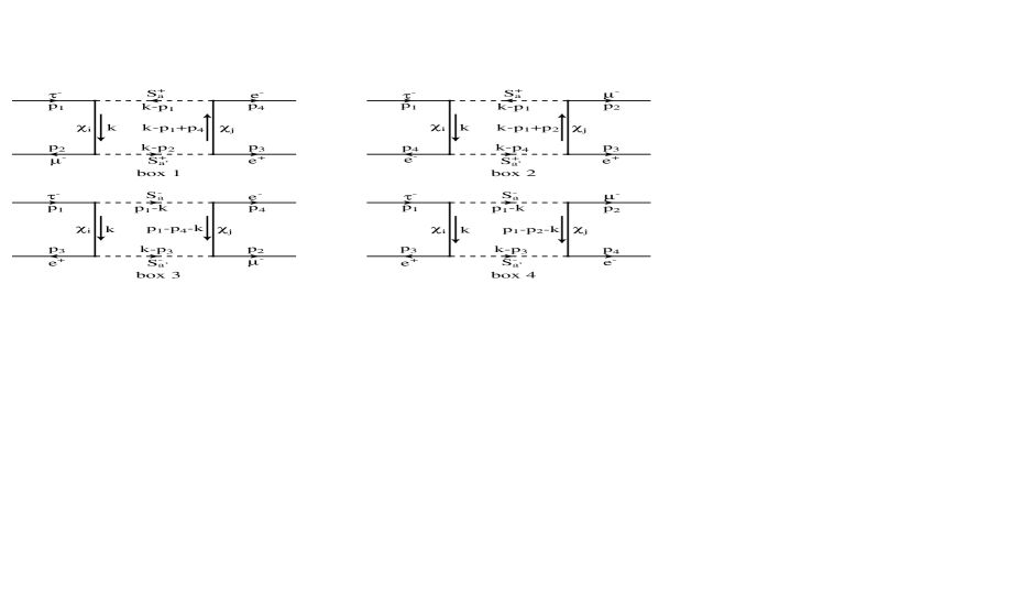
FIG. 2.: The four types of box diagrams for $\tau^{-}\to\mu^{-}e^{+}e^{-}$ which occur in our model.

Finally, the box diagram with two $W^{\pm}$ yields

$$\bar{M}_{WW} = \frac{ig^{4}}{64\pi^{2}}\sum_{i,j}\left(U_{L}\right)_{\mu i}\left(U_{L}^{\dagger}\right)_{i\tau}\left(U_{L}\right)_{ej}\left(U_{L}^{\dagger}\right)_{je}$$ (181)

$$\times\int_{0}^{1}\!dx\,\int_{0}^{1-x}\!dy\,\int_{0}^{1-x-y}\!dz\,\left[\frac{A_{ij}^{WW}}{\left(D_{ij}^{WW}\right)^{2}}-\frac{B_{ij}^{WW}}{2D_{ij}^{WW}}\right].$$

In Eqs. (177)–(181),

$$D_{ij}^{aa^{\prime}} = xm_{a}^{2}+ym_{a^{\prime}}^{2}+zm_{j}^{2}+\left(1-x-y-z\right)\left(m_{i}^{2}-xp_{1}^{2}-yp_{2}^{2}-zr^{2}\right)$$ (183)

$$-xyq^{2}-xzp_{4}^{2}-yzp_{3}^{2}\,;$$

$D_{ij}^{aW}$, $D_{ij}^{Wa^{\prime}}$, and $D_{ij}^{WW}$ are obtained from $D_{ij}^{aa^{\prime}}$ by substituting either $m_{a^{\prime}}$, or $m_{a}$, or both, by $m_{W}$. In order to write down the expressions for $A_{ij}^{aa^{\prime}},\ldots,B_{ij}^{WW}$ one must define

$$P^{\alpha} = p_{1}^{\alpha}\left(x+z\right)+p_{2}^{\alpha}y-p_{4}^{\alpha}z\,,$$ (184)

$$P^{\prime\alpha} = p_{1}^{\alpha}\left(x+z-1\right)+p_{2}^{\alpha}y+p_{4}^{\alpha}\left(1-z\right).$$ (185)

One then has

$$A_{ij}^{aa^{\prime}} = \bar{u}_{\mu}\left[\left(R_{a^{\prime}}\right)_{\mu i}\left(R_{a}^{\dagger}\right)_{i\tau}\!\!\not\!P\gamma_{L}+\left(L_{a^{\prime}}\right)_{\mu i}\left(L_{a}^{\dagger}\right)_{i\tau}\!\!\not\!P\gamma_{R}-m_{i}\left(R_{a^{\prime}}\right)_{\mu i}\left(L_{a}^{\dagger}\right)_{i\tau}\gamma_{R}\right.$$ (188)

$$\left.-m_{i}\left(L_{a^{\prime}}\right)_{\mu i}\left(R_{a}^{\dagger}\right)_{i\tau}\gamma_{L}\right]u_{\tau}\,\bar{u}_{e}\left[\left(R_{a}\right)_{ej}\left(R_{a^{\prime}}^{\dagger}\right)_{je}\!\!\not\!P^{\prime}\gamma_{L}+\left(L_{a}\right)_{ej}\left(L_{a^{\prime}}^{\dagger}\right)_{je}\!\!\not\!P^{\prime}\gamma_{R}\right.$$

$$\left.-m_{j}\left(R_{a}\right)_{ej}\left(L_{a^{\prime}}^{\dagger}\right)_{je}\gamma_{R}-m_{j}\left(L_{a}\right)_{ej}\left(R_{a^{\prime}}^{\dagger}\right)_{je}\gamma_{L}\right]v_{e}\,,$$

$$A_{ij}^{aW} = -\bar{u}_{\mu}\gamma^{\rho}\gamma_{L}\left[m_{i}\left(R_{a}^{\dagger}\right)_{i\tau}-\!\!\not\!P\!\left(L_{a}^{\dagger}\right)_{i\tau}\right]u_{\tau}\,\bar{u}_{e}\left[\left(R_{a}\right)_{ej}m_{j}-\left(L_{a}\right)_{ej}\!\!\not\!P^{\prime}\right]\gamma_{\rho}\gamma_{L}v_{e}\,,$$ (189)

$$A_{ij}^{Wa} = -\bar{u}_{\mu}\left[\left(R_{a}\right)_{\mu i}m_{i}-\left(L_{a}\right)_{\mu i}\!\!\not\!P\right]\gamma^{\rho}\gamma_{L}u_{\tau}\,\bar{u}_{e}\gamma_{\rho}\gamma_{L}\left[m_{j}\left(R_{a}^{\dagger}\right)_{je}-\!\!\not\!P^{\prime}\left(L_{a}^{\dagger}\right)_{je}\right]v_{e}\,,\hskip 14.22636pt$$ (190)

$$A_{ij}^{WW} = \bar{u}_{\mu}\gamma^{\rho}\!\!\not\!P\gamma^{\sigma}\gamma_{L}u_{\tau}\,\bar{u}_{e}\gamma_{\sigma}\!\!\not\!P^{\prime}\gamma_{\rho}\gamma_{L}v_{e}\,.$$ (191)

One obtains $B_{ij}^{aa^{\prime}}$ by discarding from $A_{ij}^{aa^{\prime}}$ all the terms which contain neither $\not\!P$ nor $\not\!P^{\prime}$, and then substituting, in the remaining terms, $\not\!P$ by $\gamma^{\theta}$ and $\not\!P^{\prime}$ by $\gamma_{\theta}$. Applying the same algorithm, one obtains $B_{ij}^{aW}$ from $A_{ij}^{aW}$, $B_{ij}^{Wa}$ from $A_{ij}^{Wa}$, and $B_{ij}^{WW}$ from $A_{ij}^{WW}$.

Next we consider the box diagrams in which the fermion line starting in the incoming $\tau^{-}$ ends in the outgoing $e^{-}$. Those are the diagrams called “box 2” in Fig. 2. The corresponding amplitudes may be obtained from Eqs. (177)–(191) by using, instead of Eqs. (183)–(185),

$$D_{ij}^{aa^{\prime}} = xm_{a}^{2}+ym_{a^{\prime}}^{2}+zm_{j}^{2}+\left(1-x-y-z\right)\left(m_{i}^{2}-xp_{1}^{2}-yp_{4}^{2}-zq^{2}\right)$$ (193)

$$-xyr^{2}-xzp_{2}^{2}-yzp_{3}^{2}\,,$$

$$P^{\alpha} = p_{1}^{\alpha}\left(x+z\right)-p_{2}^{\alpha}z+p_{4}^{\alpha}y\,,$$ (194)

$$P^{\prime\alpha} = p_{1}^{\alpha}\left(x+z-1\right)+p_{2}^{\alpha}\left(1-z\right)+p_{4}^{\alpha}y\,,$$ (195)

and by making, in Eqs. (188)–(191), the substitutions $\bar{u}_{\mu}\leftrightarrow\bar{u}_{e}$, $\left(L_{a},R_{a}\right)_{ej}\rightarrow\left(L_{a},R_{a}\right)_{\mu j}$, and $\left(L_{a,a^{\prime}},R_{a,a^{\prime}}\right)_{\mu i}\rightarrow\left(L_{a,a^{\prime}},R_{a,a^{\prime}}\right)_{ei}$. Finally, one must change the overall sign of the amplitudes, i.e. insert a minus sign in front of Eqs. (177)–(181), due to the interchange of two fermions in the final state. In Eqs. (178)–(181) one must also interchange $\left(U_{L}\right)_{\mu i}\rightarrow\left(U_{L}\right)_{ei}$ and $\left(U_{L}\right)_{ej}\rightarrow\left(U_{L}\right)_{\mu j}$.

Another type of diagrams are the box diagrams denoted “box 3” in Fig. 2. Those diagrams arise due to the Majorana character of the neutrinos, and they must be computed using specific Feynman rules for Majorana fields—see, for instance, Ref. [17]. One obtains, analogously to Eqs. (177)–(181), the following contributions to the decay (30):

$$\tilde{M}_{aa^{\prime}} = \frac{i}{16\pi^{2}}\,\int_{0}^{1}\!dx\,\int_{0}^{1-x}\!dy\,\int_{0}^{1-x-y}\!dz\,\sum_{i,j}\sum_{a,a^{\prime}}\left[\frac{\tilde{A}_{ij}^{aa^{\prime}}}{\left(\tilde{D}_{ij}^{aa^{\prime}}\right)^{2}}-\frac{\tilde{B}_{ij}^{aa^{\prime}}}{2\tilde{D}_{ij}^{aa^{\prime}}}\right],$$ (196)

$$\tilde{M}_{aW} = \frac{ig^{2}}{32\pi^{2}}\sum_{i,j}\left(U_{L}^{\dagger}\right)_{ie}\left(U_{L}\right)_{\mu j}\,\int_{0}^{1}\!dx\int_{0}^{1-x}\!dy\int_{0}^{1-x-y}\!dz\sum_{a}\left[\frac{\tilde{A}_{ij}^{aW}}{\left(\tilde{D}_{ij}^{aW}\right)^{2}}-\frac{\tilde{B}_{ij}^{aW}}{2\tilde{D}_{ij}^{aW}}\right],$$ (197)

$$\tilde{M}_{Wa} = \frac{ig^{2}}{32\pi^{2}}\sum_{i,j}\left(U_{L}^{\dagger}\right)_{i\tau}\left(U_{L}\right)_{ej}\,\int_{0}^{1}\!dx\int_{0}^{1-x}\!dy\int_{0}^{1-x-y}\!dz\sum_{a}\left[\frac{\tilde{A}_{ij}^{Wa}}{\left(\tilde{D}_{ij}^{Wa}\right)^{2}}-\frac{\tilde{B}_{ij}^{Wa}}{2\tilde{D}_{ij}^{Wa}}\right],$$ (199)

$$\tilde{M}_{WW} = \frac{ig^{4}}{64\pi^{2}}\sum_{i}m_{i}\left(U_{L}^{\dagger}\right)_{ie}\left(U_{L}^{\dagger}\right)_{i\tau}\sum_{j}m_{j}\left(U_{L}\right)_{ej}\left(U_{L}\right)_{\mu j}$$ (202)

$$\times\int_{0}^{1}\!dx\,\int_{0}^{1-x}\!dy\,\int_{0}^{1-x-y}\!dz\,\left[\frac{\tilde{A}_{ij}^{WW}}{\left(\tilde{D}_{ij}^{WW}\right)^{2}}-\frac{\tilde{B}_{ij}^{WW}}{2\tilde{D}_{ij}^{WW}}\right].$$

Here,

$$\tilde{D}_{ij}^{aa^{\prime}} = xm_{a}^{2}+ym_{a^{\prime}}^{2}+zm_{j}^{2}+\left(1-x-y-z\right)m_{i}^{2}$$ (205)

$$-x\left(1-x-z\right)p_{1}^{2}-y\left(x+z\right)p_{2}^{2}-y\left(1-y-z\right)p_{3}^{2}-x\left(y+z\right)p_{4}^{2}$$

$$+xyq^{2}+\left[xy-z\left(1-x-y-z\right)\right]r^{2}\,.$$

Notice that $\tilde{M}_{WW}$ is proportional to $m_{i}$ and to $m_{j}$, indicating that it vanishes in both limits $m_{i}\to 0$ and $m_{j}\to 0$. This is an instance of Kayser’s “practical Majorana–Dirac confusion theorem” [18]. Defining

$$\tilde{P}^{\alpha} = p_{1}^{\alpha}\left(x+z\right)+p_{3}^{\alpha}y-p_{4}^{\alpha}z\,,$$ (206)

$$\tilde{P}^{\prime\alpha} = p_{1}^{\alpha}\left(x+z-1\right)+p_{3}^{\alpha}y+p_{4}^{\alpha}\left(1-z\right)\,,$$ (207)

one may write

$$\tilde{A}_{ij}^{aa^{\prime}} = v_{e}^{T}C^{-1}\left[\left(R_{a^{\prime}}^{\dagger}\right)_{ie}\left(L_{a}^{\dagger}\right)_{i\tau}\!\!\not\!\tilde{P}\gamma_{R}+\left(L_{a^{\prime}}^{\dagger}\right)_{ie}\left(R_{a}^{\dagger}\right)_{i\tau}\!\!\not\!\tilde{P}\gamma_{L}-m_{i}\left(R_{a^{\prime}}^{\dagger}\right)_{ie}\left(R_{a}^{\dagger}\right)_{i\tau}\gamma_{L}\right.$$ (210)

$$\left.-m_{i}\left(L_{a^{\prime}}^{\dagger}\right)_{ie}\left(L_{a}^{\dagger}\right)_{i\tau}\gamma_{R}\right]u_{\tau}\,\bar{u}_{\mu}\left[\left(R_{a^{\prime}}\right)_{\mu j}\left(L_{a}\right)_{ej}\!\!\not\!\tilde{P}^{\prime}\gamma_{L}+\left(L_{a^{\prime}}\right)_{\mu j}\left(R_{a}\right)_{ej}\!\!\not\!\tilde{P}^{\prime}\gamma_{R}\right.$$

$$\left.+m_{j}\left(R_{a^{\prime}}\right)_{\mu j}\left(R_{a}\right)_{ej}\gamma_{R}+m_{j}\left(L_{a^{\prime}}\right)_{\mu j}\left(L_{a}\right)_{ej}\gamma_{L}\right]C\bar{u}_{e}^{T}\,,$$

$$\tilde{A}_{ij}^{aW} = v_{e}^{T}C^{-1}\gamma^{\rho}\gamma_{R}\left[\left(R_{a}^{\dagger}\right)_{i\tau}\!\!\not\!\tilde{P}-m_{i}\left(L_{a}^{\dagger}\right)_{i\tau}\right]u_{\tau}\,\bar{u}_{\mu}\gamma_{\rho}\gamma_{L}\left[\left(R_{a}\right)_{ej}\!\!\not\!\tilde{P}^{\prime}+\left(L_{a}\right)_{ej}m_{j}\right]C\bar{u}_{e}^{T}\,,$$ (211)

$$\tilde{A}_{ij}^{Wa} = v_{e}^{T}C^{-1}\left[\left(R^{\dagger}_{a}\right)_{ie}\!\!\not\!\tilde{P}-m_{i}\left(L^{\dagger}_{a}\right)_{ie}\right]\gamma^{\rho}\gamma_{L}u_{\tau}\,\bar{u}_{\mu}\left[\left(R_{a}\right)_{\mu j}\!\!\not\!\tilde{P}^{\prime}+\left(L_{a}\right)_{\mu j}m_{j}\right]\gamma_{\rho}\gamma_{R}C\bar{u}_{e}^{T}\,,$$ (213)

$$\tilde{A}_{ij}^{WW} = -v_{e}^{T}C^{-1}\gamma^{\rho}\gamma^{\sigma}\gamma_{L}u_{\tau}\,\bar{u}_{\mu}\gamma_{\rho}\gamma_{\sigma}\gamma_{R}C\bar{u}_{e}^{T}\,.$$ (215)

One obtains $\tilde{B}_{ij}^{aa^{\prime}}$ from $\tilde{A}_{ij}^{aa^{\prime}}$—and similarly $\tilde{B}_{ij}^{aW}$ from $\tilde{A}_{ij}^{aW}$, $\tilde{B}_{ij}^{Wa}$ from $\tilde{A}_{ij}^{Wa}$, and $\tilde{B}_{ij}^{WW}$ from $\tilde{A}_{ij}^{WW}$—by deleting all the terms which contain neither $\not\!\tilde{P}$ nor $\not\!\tilde{P}^{\prime}$, and then substituting, in the remaining terms, $\not\!\tilde{P}$ by $\gamma^{\theta}$ and $\not\!\tilde{P}^{\prime}$ by $\gamma_{\theta}$.

Finally, there are the box diagrams of the type denoted in Fig. 2 “box 4”. The corresponding amplitudes may be obtained from Eqs. (196)–(215) in the following way. Firstly, one must change the overall sign of Eqs. (196)–(202) and perform in them the interchange $\left(U_{L}\right)_{ej}\leftrightarrow\left(U_{L}\right)_{\mu j}$. Secondly, in Eqs. (205)–(207) one must interchange $p_{2}^{\alpha}\leftrightarrow p_{4}^{\alpha}$, $p_{2}^{2}\leftrightarrow p_{4}^{2}$, and $q^{2}\leftrightarrow r^{2}$. Lastly, in Eqs. (210)–(215) one must interchange $\bar{u}_{\mu}\leftrightarrow\bar{u}_{e}$ and $\left(L_{a,a^{\prime}},R_{a,a^{\prime}}\right)_{ej}\leftrightarrow\left(L_{a,a^{\prime}},R_{a,a^{\prime}}\right)_{\mu j}$.

One may analyze the $m_{R}$ dependence of the box amplitudes given above by using the skills developed in the previous sections. It is easily concluded that all those amplitudes are suppressed by at least one factor $m_{R}^{-2}$. In order to reach this conclusion, it is necessary to use Eq. (86), when the box diagrams are either of type “box 1” or “box 2” and both $\chi_{i}$ and $\chi_{j}$ are light neutrinos.

X The asymptotic limit $m_{R}\to\infty$

In our model there is a scale $m_{R}$ which is much higher than the other two scales, $m_{D}$ and $m_{F}$ (see Section IV). In this section we want to study the asymptotic limit $m_{R}\to\infty$ of our model. The simplest way—the one which we have in mind in the following—of increasing the scale $m_{R}$ is by multiplying the mass matrix $M_{R}$ in Eq. (4) by a (dimensionless) factor which becomes much larger than one.

When the decoupling theorem [19, 20] applies straightforwardly, one may simply delete the heavy fields from the Lagrangian in order to obtain the low-energy theory. In our case this does not work because, if we remove the fields $\nu_{R}$ from the Lagrangian, we also delete any trace of the flavor-changing neutral interactions. This is at odds with the explicit one-loop calculation of the vertex $\ell\to\ell^{\prime}{S_{b}^{0}}^{\ast}$, for $\ell\neq\ell^{\prime}$, since that vertex does not vanish in the limit $m_{R}\to\infty$ (see Fig. 1 for the Feynman diagrams with non-vanishing contributions). On the other hand, according to Ref. [20], the limit $m_{R}\to\infty$ must yield a sensible theory. Evidently, the only theory which can emerge from our model in that limit is the multi-Higgs-doublet SM, containing flavor-changing neutral Higgs interactions suppressed by loop factors $16\pi^{2}$ and by small couplings. Thus, we expect a Yukawa Lagrangian of the form

$$\tilde{\mathcal{L}}_{\mathrm{Y}}=-\sum_{j=1}^{n_{H}}\left(\begin{array}[]{cc}\varphi_{j}^{-}\,,&{\varphi_{j}^{0}}^{\ast}\end{array}\right)\bar{\ell}_{R}\,\tilde{\Gamma}_{j}\left(\begin{array}[]{c}\tilde{\nu}_{L}\\ \ell_{L}\end{array}\right)+\mathrm{H.c.}$$ (216)

In order to demonstrate that this Lagrangian indeed emerges, we consider the following couplings:

1. $\ell_{L}\to\ell^{\prime}_{R}{S^{0}}^{\ast}$,

2. $\nu_{L}\to\ell_{R}{S^{+}}^{\ast}$,

3. $\nu_{L}\to\ell_{L}{W^{+}}^{\ast}$.

For the sake of brevity, let us denote the corresponding tree-level vertices by $V_{0}$, $V_{+}$, and $V_{W}$, respectively. The one-loop contributions to these vertices fall into three categories:

1. The contribution has a non-vanishing limit $m_{R}\to\infty$.

2. In the limit $m_{R}\to\infty$ the contribution vanishes.

3. The contribution is independent of $m_{R}$ and is present also when the fields $\nu_{R}$ are removed from the Lagrangian.

Our strategy is the following. We identify all contributions of Category I, since only they are relevant for obtaining the limit $m_{R}\to\infty$ of our model. We then show that there are three contributions of Category I to $V_{W}$, but they cancel out except for a part which may be viewed as a unitary transformation on the vector of flavor fields $\nu_{L}$. The transformed field vector is denoted by $\tilde{\nu}_{L}$. After these steps, we see that the contributions of Category I to the vertices $V_{0}$ and $V_{+}$ are identical, provided that the neutrino field $\tilde{\nu}_{L}$ is used in $V_{+}$. This demonstrates that in the limit $m_{R}\to\infty$ the Yukawa Lagrangian of Eq. (216) emerges. After the one-loop corrections, as discussed above, we remove the fields $\nu_{R}$ from the Lagrangian. Then all the traces left by those heavy fields are contained in the off-diagonal elements of $\tilde{\Gamma}_{j}$, which have arisen from the one-loop corrections of Category I.

We now pursue the strategy outlined in the previous paragraph. First consider the vertex and self-energy corrections for the above couplings:

$$V_{0}: \Gamma_{k}+\Delta\Gamma_{k}\left(V_{0},S^{\pm}\right)+\frac{1}{2}\left[z_{R}^{\ell}\left(S^{\pm}\right)\right]^{\dagger}\Gamma_{k}+\frac{1}{2}\,\Gamma_{k}z_{L}^{\ell}\left(S^{\pm}\right),$$ (217)

$$V_{+}: \Gamma_{k}+\Delta\Gamma_{k}\left(V_{+},S^{0}\right)+\frac{1}{2}\left[z_{R}^{\ell}\left(S^{\pm}\right)\right]^{\dagger}\Gamma_{k}+\frac{1}{2}\,\Gamma_{k}z_{L}^{\nu}\left(S^{0}\right)\,,$$ (218)

$$V_{W}: \frac{g}{\sqrt{2}}\left\{1+\Gamma\left(V_{W},S\right)+\frac{1}{2}\left[z_{L}^{\ell}\left(S^{\pm}\right)\right]^{\dagger}+\frac{1}{2}\,z_{L}^{\nu}\left(S^{0}\right)\right\}.$$ (219)

For the definition of the wave-function renormalization matrices $z_{L}^{\ell}$, $z_{R}^{\ell}$, and $z_{L}^{\nu}$ see Appendix B. It is proven by a tedious checking of all one-loop graphs that the corrections to $V_{0}$, $V_{+}$, and $V_{W}$ not included in Eqs. (217), (218), and (219), respectively, are either of Category II or Category III. In the expressions (218) and (219), only one-loop corrections in which the external neutrino legs correspond to light neutrinos are interesting. Those one-loop corrections are obtained by performing the calculations with the fields $\chi_{i}$, but the result has to be multiplied appropriately by $U_{L}$; in order to obtain $\Delta\Gamma_{k}(V_{+},S^{\pm})$ a multiplication from the right by $U_{L}^{\dagger}$ is necessary; the $6\times 6$ matrix part of the neutrino self-energy associated with the Dirac structure $p\hskip-5.0pt/\gamma_{L}$ has to be multiplied by $U_{L}$ from the left and $U_{L}^{\dagger}$ from the right in order to arrive at the $3\times 3$ matrix we need; and so on. With this procedure we have in mind that, in the limit $m_{R}\to\infty$, the light neutrinos become massless, and we are allowed to work with the fields $\nu_{L}$, which are members of the left-handed lepton doublets in the Lagrangian before spontaneous symmetry breaking. In the following, our results for the quantities appearing in Eqs. (217), (218), and (219) will only be given for $m_{R}\to\infty$, since this is the limit we aim at. In Eq. (217) the vertex correction $\Delta\Gamma_{k}(V_{0},S^{\pm})$ is obtained by exchanging all charged scalars, including the charged Goldstone boson $G^{\pm}$. In Eq. (218) the vertex correction $\Delta\Gamma_{k}(V_{+},S^{0})$ stems from exchanging all neutral scalars, including the neutral Goldstone boson $G^{0}$. The vertex correction $\Gamma(V_{W},S)$ originates in the coupling of the W boson to a charged and a neutral scalar; thus, the loop has $S^{0}_{b}$, $S^{\pm}_{a}$, and $\chi_{i}$. Concerning the wave-function renormalization matrices $z_{L}^{\ell}(S^{\pm})$, $z_{R}^{\ell}(S^{\pm})$, and $z_{L}^{\nu}(S^{0})$, in parentheses we have indicated the scalar exchange they come from in the self-energies.

In Eqs. (217), (218), and (219), all the one-loop contributions which occur contain two $\Delta$ and one $\Gamma$ Yukawa-coupling matrices. The vertices $V_{0}$ and $V_{+}$ also receive contributions from the wave-function renormalization matrix of the Higgs doublets; these contributions fall into all three categories. One can show that those of Category I induce the same corrections to $\Gamma_{k}$ at the vertices $V_{0}$ and $V_{+}$.

Before we list the one-loop results for the quantities appearing in Eqs. (217), (218), and (219), we want to introduce some useful notation. First we note that

$$\lim_{m_{R}\to\infty}U_{R}=(0,W)\,,\quad\lim_{m_{R}\to\infty}m_{1,2,3}=0\,,$$ (220)

where $W$ is a $3\times 3$ unitary matrix. We define a useful $3\times 3$ Hermitian matrix by

$$A\equiv\frac{1}{16\pi^{2}}\sum_{j=1}^{n_{H}}\Delta_{j}^{\dagger}\left[-\frac{1}{2}\,\mathcal{K}-\frac{3}{4}+\frac{1}{2}\,W\ln{\tilde{m}}^{2}\,W^{\dagger}\right]\Delta_{j}\,,$$ (221)

where the divergent constant $\mathcal{K}$ has been defined in Eq. (43) and

$$\tilde{m}=\mathrm{diag}\left(m_{4},m_{5},m_{6}\right).$$ (222)

Then, it is easy to write down the self-energy

$$\Sigma_{\nu}^{\infty}\left(S^{0};p\right)=Ap\hskip-5.0pt/\gamma_{L}$$ (223)

for the neutrinos, and

$$\Sigma_{\ell}^{\infty}\left(S^{\pm};p\right)=Ap\hskip-5.0pt/\gamma_{L}+B\gamma_{L}+B^{\dagger}\gamma_{R}$$ (224)

for the charged leptons, with $B$ given by

$$B=\frac{1}{16\pi^{2}}\sum_{j=1}^{n_{H}}\Gamma_{j}\left[M_{D}^{\dagger}\left(\mathcal{K}+1\right)-W\tilde{m}\ln{\tilde{m}^{2}}W^{\dagger}\right]\Delta_{j}\,.$$ (225)

The superscript $\infty$ reminds us that we have taken the limit $m_{R}\to\infty$. In the same limit, the vertex corrections are given by

$$\Delta\Gamma_{k}\left(V_{0},S^{\pm}\right)=\Delta\Gamma_{k}\left(V_{+},S^{0}\right)=\frac{1}{16\pi^{2}}\sum_{j=1}^{n_{H}}\Gamma_{j}\Delta_{k}^{\dagger}\left(\mathcal{K}+1-W\ln{\tilde{m}^{2}}W^{\dagger}\right)\Delta_{j}$$ (226)

and

$$\Gamma\left(V_{W},S\right)=-A\,.$$ (227)

The off-diagonal elements of $\Delta\Gamma_{k}(V_{0},S^{\pm})$ are given by the vertex correction computed in Section VIII, in the limit $m_{R}\to\infty$; the same holds for $\Sigma_{\ell}^{\infty}(S^{\pm};p)$. In order to calculate the self-energy (223) one has to take into account the Majorana nature of the fields $\chi_{i}$: the neutrino self-energy derives from a propagator at second order in perturbation theory, and there are $2^{3}=8$ possibilities to attach the external legs to neutrino fields in the two $S^{0}$ Yukawa Lagrangians; therefore there is a combinatorial factor $2^{3}/2!=4$. Furthermore, the terms $B_{L,R}$ drop out of the neutrino self-energy because of [14]

$$\sum_{b}b_{k}b_{k^{\prime}}=0\,.$$ (228)

We have also used the relations (see Appendix A.1)

$$\sum_{b}b_{k}^{\ast}b_{k^{\prime}}=2\sum_{a}a_{k}^{\ast}a_{k^{\prime}}=2\delta_{kk^{\prime}}\,,$$ (229)

which have enabled us to sum, in Eqs. (221), (225) and (226) over the index $j$.

Since in the limit $m_{R}\to\infty$ the neutrinos are massless, the procedure for the renormalization of the self-energy laid out in Appendix B.1 is not applicable. However, it is reasonable, in view of Eq. (223), to define

$$z_{R}^{\nu}\left(S^{0}\right)=0\,,\quad z_{L}^{\nu}\left(S^{0}\right)=\left[z_{L}^{\nu}\left(S^{0}\right)\right]^{\dagger}=A\,.$$ (230)

The determination of $z_{L}^{\ell}$ and of $z_{R}^{\ell}$ follows the on-shell prescription in Appendix B.1.

In the expression for the one-loop correction of $V_{W}$, Eq. (219), the only matrix which is possibly non-Hermitian is $z_{L}^{\ell}(S^{\pm})$. In any case, we may decompose that matrix into a Hermitian and an anti-Hermitian part:

$$z_{L}^{\ell}\left(S^{\pm}\right)=z_{+}^{\ell}+z_{-}^{\ell}\,,\quad\mathrm{with}\quad\left(z_{\pm}^{\ell}\right)^{\dagger}=\pm z_{\pm}^{\ell}\,.$$ (231)

We notice that in the $\Sigma_{\ell}^{\infty}(S^{\pm};p)$ of Eq. (224) there is no term $A_{R}^{\ell}p\hskip-5.0pt/$. Using the equations in Appendix B.1 for calculating the fermion wave-function renormalization matrices, this fact simplifies considerably the expression for $z^{\ell}_{L,R}$. Since $A$ is Hermitian, we obtain

$$\mathrm{Re}\left[z_{L}^{\ell}\left(S^{\pm}\right)-z_{R}^{\ell}\left(S^{\pm}\right)\right]_{\alpha\alpha}=A_{\alpha\alpha}\,,\quad\mathrm{Im}\left[z_{L}^{\ell}\left(S^{\pm}\right)-z_{R}^{\ell}\left(S^{\pm}\right)\right]_{\alpha\alpha}=-\frac{2}{m_{\alpha}}\mathrm{Im}\,B_{\alpha\alpha}\,,$$ (232)

and

$$\mathrm{Re}\left[z_{L}^{\ell}\left(S^{\pm}\right)+z_{R}^{\ell}\left(S^{\pm}\right)\right]_{\alpha\alpha}=A_{\alpha\alpha}\,.$$ (233)

Using the possibility to choose the convention

$$\mathrm{Im}\left[z_{L}^{\ell}\left(S^{\pm}\right)\right]_{\alpha\alpha}=0\,,$$ (234)

as explained at the end of Appendix B 1, we obtain $[z_{L}^{\ell}(S^{\pm})]_{\alpha\alpha}=(z_{+}^{\ell})_{\alpha\alpha}=A_{\alpha\alpha}$ and $(z_{-}^{\ell})_{\alpha\alpha}=0$. For $\alpha\neq\beta$ we apply again the procedure of Appendix B.1 and obtain $(z_{+}^{\ell})_{\beta\alpha}=A_{\beta\alpha}$. In summary, with the convention of Eq. (234) we find

$$z_{+}^{\ell}=A$$ (235)

and, with Eqs. (227) and (230),

$$\Gamma\left(V_{W},S\right)+\frac{1}{2}\left(z_{+}^{\ell}+z_{L}^{\nu}\right)=0\,.$$ (236)

Thus, Eq. (219) is given by

$$\frac{g}{\sqrt{2}}\left(1-\frac{1}{2}z_{-}^{\ell}\right).$$ (237)

Since the light-neutrino masses vanish when $m_{R}\to\infty$, we are allowed to rotate $\nu_{L}$ unitarily. An infinitesimal unitary rotation is given by

$$\nu_{L}=\left(1+\Omega\right){\tilde{\nu}}_{L}\,,\quad\mathrm{with}\quad\Omega^{\dagger}=-\Omega\,.$$ (238)

With the choice [21]

$$\Omega=\frac{1}{2}\,z_{-}^{\ell}\,,$$ (239)

the one-loop-corrected W vertex of Eq. (219) reduces to the trivial form $g/\sqrt{2}$, if conceived as pertaining to ${\tilde{\nu}}_{L}$.

In terms of the new field $\tilde{\nu}_{L}$, the vertex $V_{+}$ is given by

$$\Gamma_{k}+\Delta\Gamma_{k}\left(V_{+},S^{0}\right)+\frac{1}{2}\left[z_{R}^{\ell}\left(S^{\pm}\right)\right]^{\dagger}\Gamma_{k}+\frac{1}{2}\,\Gamma_{k}\left[z_{L}^{\nu}\left(S^{0}\right)+z_{-}^{\ell}\right].$$ (240)

Since

$$z_{L}^{\nu}\left(S^{0}\right)+z_{-}^{\ell}=A+z_{-}^{\ell}=z_{L}^{\ell}\left(S^{\pm}\right),$$ (241)

and because of Eq. (226), the expression (240) for the charged-scalar vertex is identical with the expression (217) for the neutral-scalar vertex. Therefore, in the $\tilde{\nu}_{L}$ basis for the neutrino fields, the one-loop corrections—associated with $\nu_{R}$—to the couplings of types $\bar{\ell}_{R}\ell_{L}S^{0}$ and $\bar{\ell}_{R}\tilde{\nu}_{L}S^{-}$ are identical. This is crucial for writing the theory after decoupling of the heavy fields $\nu_{R}$ as a multi-Higgs-doublet Standard Model with the Yukawa Lagrangian of Eq. (216). The coupling matrices $\tilde{\Gamma}_{k}$ are then given by Eq. (217). The infinities introduced by the one-loop contributions of Category I are all in the diagonal—see Eq. (226)—and they may, therefore, be absorbed by redefining the diagonal matrices $\Gamma_{k}$ as renormalized coupling matrices. This concludes our argument, valid at least at the one-loop level, that in the asymptotic limit $m_{R}\to\infty$ one obtains the Lagrangian of Eq. (216) and our model approaches a multi-scalar-doublet SM with suppressed off-diagonal couplings in $\tilde{\Gamma}_{j}$.

Several remarks are in order. First, we stress that the contributions to $z_{L}^{\ell}$ from $S^{0}$ exchange, and those to $z_{L}^{\nu}$ from $S^{\pm}$ exchange, are flavor-diagonal and Hermitian and, therefore, they do not have anti-Hermitian components which would interfere with the arguments presented above. This must be so because these contributions belong to Category III. Second, though in the limit of infinite right-handed scale we were able to show—taking into account a rotation of $\nu_{L}$—that the one-loop contributions of the right-handed neutrino singlets are the same for couplings of the types $\bar{\ell}_{R}\ell_{L}S^{0}$ and $\bar{\ell}_{R}\tilde{\nu}_{L}S^{-}$, this does not happen with contributions of Category III, due to the different mass effects of charged leptons and of massless neutrinos; thus, the fully one-loop-corrected coupling matrices $\Gamma_{k}$ do receive different finite parts in the $\bar{\ell}_{R}\ell_{L}S^{0}$ and $\bar{\ell}_{R}\tilde{\nu}_{L}S^{-}$ couplings because of contributions of Category III, an effect which is to be expected in the multi-scalar-doublet SM. Of course, the infinite corrections to couplings of both types are the same, which allows for a consistent renormalization procedure. Third, because of the cancellation in Eq. (236), the infinities at the vertex $V_{W}$ stemming from scalar corrections of Category I also cancel. This is necessary for consistency, since it would be impossible to absorb those infinities into the gauge coupling constant.

XI Decay rates

Experimental bounds on lepton-flavor-changing processes are found in Ref. [22]. For the $\tau$ the bounds on the branching ratios are of order $10^{-6}$, but for $\mu$ decays they are five to six orders of magnitude better. Of course, all our formulas are easily adapted to muon decays.

In this section we shall always neglect the masses of all final-state fermions. Pursuing the philosophy laid out in Section IV, we shall also assume that Yukawa couplings are of order $Y\sim m_{D}/m_{F}$, cf. Eq. (45).

First we consider the process $\tau^{-}\to\mu^{-}\gamma$. Its matrix element may be written

$$\mathcal{A}\left(\tau^{-}\to\mu^{-}\gamma\right)=e\,\varepsilon_{\rho}^{\ast}\,\bar{u}_{\mu}i\sigma^{\rho\lambda}q_{\lambda}\left(A^{\gamma}_{L}\gamma_{L}+A^{\gamma}_{R}\gamma_{R}\right)u_{\tau}\,,$$ (242)

where $\varepsilon$ is the polarization vector of the photon. Then the decay rate is

$$\Gamma\left(\tau^{-}\to\mu^{-}\gamma\right)=\Gamma_{\tau}\,\frac{48\pi^{3}\alpha}{G_{F}^{2}m_{\tau}^{2}}\left(\left|A^{\gamma}_{L}\right|^{2}+\left|A^{\gamma}_{R}\right|^{2}\right),$$ (243)

where $\alpha$ is the electromagnetic fine-structure constant, $G_{F}$ is the Fermi constant, and

$$\Gamma_{\tau}\equiv\Gamma\left(\tau^{-}\to e^{-}\bar{\nu}_{e}\nu_{\tau}\right)=\frac{G_{F}^{2}m_{\tau}^{5}}{192\pi^{3}}\,.$$ (244)

The amplitudes in Eq. (242) are given in our model by Eqs. (LABEL:alphaLi) and (LABEL:alphaRi):

$$A^{\gamma}_{L,R}=\sum_{i}\alpha_{L,Ri}\left(q^{2}=0\right).$$ (245)

In Subsection VI B we have made for those amplitudes the order-of-magnitude estimate $A^{\gamma}_{L,R}\sim Y^{2}m_{D}/(16\pi^{2}m_{R}^{2})$. Thus, the branching ratio should be of order $\alpha Y^{4}/(\pi G_{F}^{2}m_{R}^{4})$, where we have used $m_{\tau}\sim m_{D}$. With $G_{F}\approx 10^{-5}$ GeV^-2 and $m_{R}\sim 10^{10}$ GeV, we see that the branching ratio would be $\sim 10^{-32}$ even if we allowed $Y$ to be of order 1.

Next we consider the lepton-flavor-changing $Z$ decay $Z\to\tau^{+}\mu^{-}$. Its decay amplitude may be written

$$\mathcal{A}\left(Z\to\tau^{+}\mu^{-}\right)=\frac{ig}{2c_{w}}\,\varepsilon^{\rho}\,\bar{u}_{\mu}\gamma_{\rho}\left(A^{Z}_{L}\gamma_{L}+A^{Z}_{R}\gamma_{R}\right)v_{\tau}\,,$$ (246)

where $\varepsilon$ now denotes the $Z$ polarization vector. The decay rate is then

$$\Gamma\left(Z\to\tau^{+}\mu^{-}\right)=\frac{g^{2}m_{Z}}{96\pi c_{w}^{2}}\left(\left|A^{Z}_{L}\right|^{2}+\left|A^{Z}_{R}\right|^{2}\right).$$ (247)

The amplitudes $A^{Z}_{L,R}$ can be read off from $\sum_{\iota=1}^{4}M^{\rho}_{Z\iota}$, computed in Section VII. As they are of order $m_{D}^{2}/m_{R}^{2}$, once again one finds a ridiculously small decay rate.

We now discuss neutral-scalar decay, which is not suppressed by inverse powers of $m_{R}$ whenever $n_{H}\geq 2$. The matrix element is

$$\mathcal{A}\left(S_{b}^{0}\to\tau^{+}\mu^{-}\right)=\bar{u}_{\mu}\left(A^{b}_{L}\gamma_{L}+A^{b}_{R}\gamma_{R}\right)v_{\tau}\,.$$ (248)

Then the decay rate is

$$\Gamma\left(S_{b}^{0}\to\tau^{+}\mu^{-}\right)=\frac{m_{b}}{16\pi}\left(\left|A^{b}_{L}\right|^{2}+\left|A^{b}_{R}\right|^{2}\right).$$ (249)

In our model we may identify

$$A^{b}_{L}\gamma_{L}+A^{b}_{R}\gamma_{R}=\tilde{M}_{b}^{\infty}\,,$$ (250)

with $\tilde{M}_{b}^{\infty}$ given by Eq. (175) without the spinors. This is not suppressed by any power of $m_{R}^{-1}$ but it contains three Yukawa couplings. Thus, the decay rate should in general be very small due to a factor $Y^{6}/(16\pi^{2})^{2}$. In any case this is not very interesting, since no fundamental neutral scalar as been observed up to now.

Finally we consider our model process $\tau^{-}\to\mu^{-}e^{+}e^{-}$. Rather general formulas for the decay rate can be found in Refs. [11, 12]. Comparing our result of Section VI for the photon sub-process with the results in Ref. [11], we conclude that this contribution has a branching ratio of order $[\alpha^{2}/(G_{F}^{2}m_{R}^{4})](m_{D}/m_{F})^{4}/16\pi^{2}$. In the $Z$ sub-process (Section VII), $W$ exchange dominates over the exchange of charged scalars. Thus we estimate for the branching ratio of this sub-process $[\alpha_{w}^{4}/(G_{F}^{2}m_{R}^{4})](m_{D}/m_{Z})^{4}$ (of course, $m_{Z}\sim m_{F}$), where $\alpha_{w}=g^{2}/(4\pi)$ is the weak fine-structure constant. A similar suppression is found for the box sub-process of Section IX. Therefore we may safely neglect all those contributions, including interference terms, and concentrate only on the neutral-scalar sub-process computed in Section VIII. The amplitude is then written

$$\mathcal{A}\left(\tau^{-}\to\mu^{-}e^{+}e^{-}\right)=\sum_{b}\bar{u}_{\mu}\left(\lambda_{b}\gamma_{L}+\rho_{b}\gamma_{R}\right)u_{\tau}\,\bar{u}_{e}\left(\Gamma_{b}\gamma_{L}+\Gamma_{b}^{\ast}\gamma_{R}\right)v_{e}\,,$$ (251)

which is modeled according to Eq. (48). Thus, we are making the identifications $\Gamma_{b}=(\Gamma_{b})_{ee}$ and, assuming more than one scalar doublet,

$$\bar{u}_{\mu}\left(\lambda_{b}\gamma_{L}+\rho_{b}\gamma_{R}\right)u_{\tau}=-\frac{M_{b}^{\infty}}{\sqrt{2}\,m_{b}^{2}}\,,$$ (252)

where we have used the approximation $q^{2}\ll m_{b}^{2}$. From Eq. (251) one obtains

$$\frac{\Gamma\left(\tau^{-}\to\mu^{-}e^{+}e^{-}\right)}{\Gamma_{\tau}}=\frac{1}{32\,G_{F}^{2}}\left(\left|\sum_{b}\lambda_{b}\Gamma_{b}\right|^{2}+\left|\sum_{b}\lambda_{b}\Gamma_{b}^{\ast}\right|^{2}+\left|\sum_{b}\rho_{b}\Gamma_{b}\right|^{2}+\left|\sum_{b}\rho_{b}\Gamma_{b}^{\ast}\right|^{2}\right).$$ (253)

Both $\rho_{b}$ and $\lambda_{b}$ are of the form $Y^{3}/(16\pi^{2}m_{H}^{2})$, where $m_{H}$ is a typical neutral-scalar mass, which should be of order $m_{F}$. Therefore, the order of magnitude of the part of the branching ratio which is not suppressed by powers of $m_{R}$ is $Y^{8}/(16\pi^{2}G_{F}m_{F}^{2})^{2}$. With $16\pi^{2}G_{F}m_{F}^{2}\sim 10$ and $Y\sim 10^{-2}$ as reasonable numerical values, this branching ratio is quite small, of order $10^{-18}$, yet it is much larger than the photon, $Z$, and box contributions, which are all suppressed by $m_{R}^{-4}$. Due to the dependence on $Y^{8}$, we can easily achieve a branching ratio much larger than $10^{-18}$ by moderately increasing $Y$. However, in this case it is certainly not possible to allow for $Y\sim 1$. In particular, if we apply the present estimate to the branching ratio of $\mu^{-}\to e^{-}e^{+}e^{-}$, we rather find $Y^{8}\lesssim 10^{-10}$.

XII Conclusions

In this paper we have computed the amplitude of the lepton-flavor-violating decay $\tau^{-}\to\mu^{-}e^{+}e^{-}$ in the context of the seesaw model with an arbitrary number $n_{H}$ of Higgs doublets, but with the assumption that the (tree-level) Yukawa couplings conserve lepton flavor. Our calculation is easily adapted to other lepton-flavor-violating decays of the same type, e.g. $\mu^{-}\to e^{-}e^{+}e^{-}$; moreover, the parts of the calculation in which $\tau^{-}\to\mu^{-}e^{+}e^{-}$ proceeds via an intermediate photon or an intermediate $Z$ boson are also applicable to lepton-flavor-changing decays like $\tau^{\pm}\to\mu^{\pm}\gamma$ and $Z\to\tau^{\pm}\mu^{\mp}$, respectively. As a function of the right-handed scale $m_{R}$ we have found the following behavior of the decay amplitudes:

$$\mathcal{A}(\tau^{-}\to\mu^{-}\gamma) \propto 1/m_{R}^{2}\,,$$ (254)

$$\mathcal{A}(Z\to\tau^{+}\mu^{-}) \propto 1/m_{R}^{2}\,,$$ (255)

$$\mathcal{A}(\tau^{-}\to\mu^{-}e^{+}e^{-}) \propto \left\{\begin{array}[]{ll}1/m_{R}^{2}&\mathrm{for}\quad n_{H}=1\,,\\ \mathrm{constant}&\mathrm{for}\quad n_{H}>1\,.\end{array}\right.$$ (258)

The partial amplitudes for $\tau^{-}\to\mu^{-}e^{+}e^{-}$ which behave like $m_{R}^{-2}$ are, in general, suppressed by at least a factor $m_{D}m_{F}/m_{R}^{2}\sim 10^{-18}$; here we have assumed that the elements of the Dirac neutrino mass matrix $M_{D}$ are of order $m_{D}\sim 1$ GeV, the Fermi scale is of order $m_{F}\sim 100$ GeV, and $m_{R}\sim 10^{10}$ GeV. The exception to this suppression occurs precisely when there is more than one scalar doublet, for then there are contributions to $\tau^{-}\to\mu^{-}{S^{0}_{b}}^{\ast}$, where $S^{0}_{b}$ is a neutral scalar, which are not suppressed by inverse powers of $m_{R}$. These unsuppressed contributions originate from exchange of the charged scalars $S_{a}^{\pm}$; the corresponding Feynman diagrams are shown in Fig. 1. We have found that the vertices $\tau^{-}\to\mu^{-}\gamma^{\ast}$ and $\tau^{-}\to\mu^{-}Z^{\ast}$ (and therefore also the decay amplitudes for $\tau^{-}\to\mu^{-}\gamma$ and $Z\to\tau^{+}\mu^{-}$), which had already been computed before by other authors in the case of only one scalar doublet, are, even in the case of many doublets, suppressed by $m_{D}^{2}/m_{R}^{2}\sim 10^{-20}$. Furthermore, also the box diagrams behave like $1/m_{R}^{2}$ for an arbitrary $n_{H}$. Therefore, with the above numerical assumptions, all classes of diagrams, except those with intermediate neutral scalars in the case of more than one Higgs doublet, are basically irrelevant for the process (30).

The unsuppressed contribution to the vertex $\tau^{-}\to\mu^{-}{S^{0}_{b}}^{\ast}$ is found in Eq. (175), with the quantities $A_{L}$ and $A_{R}$ given by Eqs. (141) and (143), respectively. That unsuppressed contribution has three Yukawa couplings and a denominator $16\pi^{2}$; if we assume each Yukawa coupling to be of order $m_{D}/m_{F}\sim 10^{-2}$, we obtain an overall order of magnitude $10^{-8}$. This is certainly very small, but anyway much larger than anything which is suppressed by $m_{R}^{-2}$. Moreover, we may allow for Yukawa couplings larger than $10^{-2}$.

Estimating the branching ratio for the non-suppressed decay $\tau^{-}\to\mu^{-}e^{+}e^{-}$, we obtain [7] $Y^{8}/\left(16\pi^{2}G_{F}m_{H}^{2}\right)^{2}\sim 10^{-18}$, where we have taken $m_{H}\sim m_{F}$ for a typical neutral-scalar mass, $Y\sim m_{D}/m_{F}$ for a typical Yukawa coupling, and with the same assumptions as before for the scales $m_{D}$, $m_{F}$, and $m_{R}$. This branching ratio, valid for $n_{H}>1$, is not suppressed by the large scale $m_{R}$, but it is suppressed instead by the eighth power of a typical Yukawa coupling $Y$. We want to stress, however, that the estimate $10^{-18}$ for the branching ratio of $\tau^{-}\to\mu^{-}e^{+}e^{-}$ is rather crude; having in mind the remarks at the end of the previous paragraph, it could easily be several orders of magnitude larger due to its dependence on $Y^{8}$. On the other hand, the branching ratio for $\tau^{-}\to\mu^{-}\gamma$ is suppressed by $\alpha Y^{4}/(\pi G_{F}^{2}m_{R}^{4})\sim 10^{-40}$.

We have studied in detail the non-decoupling in the Higgs sector for $m_{R}\to\infty$. In this limit our model approaches a multi-Higgs-doublet Standard Model with lepton-flavor non-diagonal Yukawa couplings, the off-diagonal couplings being, however, suppressed. The situation here reminds somehow the Minimal Supersymmetric Standard Model, which has two Higgs doublets, where non-decoupling in the Higgs sector has been found when the SUSY scale is made much larger than the Fermi scale but the masses of all scalars are kept of order $m_{F}$ [23].

The model discussed here with lepton-flavor-diagonal Yukawa couplings was put forward in Ref. [7] as a framework for imposing large or maximal neutrino mixing. Here we have shown in a detailed way that, despite the soft breaking of the lepton numbers at the very large scale $m_{R}$, the branching ratios of lepton-flavor-violating processes remain very small. We have identified the class of processes whose vertices are not suppressed by $m_{R}^{-2}$. In this class the most promising example for future experiments is $\mu^{-}\to e^{-}e^{+}e^{-}$; this non-suppression requires more than one Higgs doublet. Those vertices suppressed by $m_{R}^{-2}$ lead to branching ratios far beyond present or future experimental limits. Thus we have a viable model with the interesting feature that neutrino mixing has its origin at the ultra-high scale $m_{R}$—the order of magnitude of the masses of the right-handed neutrino singlets, which is at the same time, via the seesaw mechanism, responsible for the smallness of the light-neutrino masses.

A Formalism for the scalar sector

1 $S_{a}^{\pm}$ and $S_{b}^{0}$

We allow for an arbitrary number $n_{H}$ of scalar doublets $\phi_{k}$ ($k=1,2,\ldots,n_{H}$) and use the notation

$$\phi_{k}=\left(\begin{array}[]{c}\varphi_{k}^{+}\\ \varphi_{k}^{0}\end{array}\right),\quad\mathrm{with}\quad\left\langle 0\left|\varphi_{k}^{0}\right|0\right\rangle=\frac{v_{k}}{\sqrt{2}}\,.$$ (A1)

We then write

$$\varphi^{0}_{k}=\frac{v_{k}}{\sqrt{2}}+{\varphi^{0}_{k}}^{\hskip 1.0pt\raisebox{-1.0pt}{$\scriptstyle\prime$}}\,,\quad\mbox{hence}\quad\left\langle 0\left|{\varphi^{0}_{k}}^{\hskip 1.0pt\raisebox{-1.0pt}{$\scriptstyle\prime$}}\right|0\right\rangle=0\,.$$ (A2)

The quadratic terms in the scalar potential are written

$$V_{\mathrm{mass}}=\sum_{i,j}\left[\varphi^{-}_{i}\left(\mathcal{M}^{2}_{+}\right)_{ij}\,\varphi^{+}_{j}+A_{ij}\,\mbox{Re}\,{\varphi^{0}_{i}}^{\hskip 1.0pt\raisebox{-1.0pt}{$\scriptstyle\prime$}}\,\mbox{Re}\,{\varphi^{0}_{j}}^{\hskip 1.0pt\raisebox{-1.0pt}{$\scriptstyle\prime$}}+B_{ij}\,\mbox{Im}\,{\varphi^{0}_{i}}^{\hskip 1.0pt\raisebox{-1.0pt}{$\scriptstyle\prime$}}\,\mbox{Im}\,{\varphi^{0}_{j}}^{\hskip 1.0pt\raisebox{-1.0pt}{$\scriptstyle\prime$}}+2C_{ij}\,\mbox{Re}\,{\varphi^{0}_{i}}^{\hskip 1.0pt\raisebox{-1.0pt}{$\scriptstyle\prime$}}\,\mbox{Im}\,{\varphi^{0}_{j}}^{\hskip 1.0pt\raisebox{-1.0pt}{$\scriptstyle\prime$}}\right].$$ (A3)

The matrix $\mathcal{M}^{2}_{+}$ is complex and Hermitian, while the matrices $A$ and $B$ are real and symmetric; $C$ is real but otherwise arbitrary. They are all $n_{H}\times n_{H}$ matrices. The eigenvalue equations are

$$\mathcal{M}^{2}_{+}\,a = m_{a}^{2}\,a\,,$$ (A4)

$$\mathcal{M}^{2}_{0}\left(\begin{array}[]{c}\mbox{Re}\,b\\ \mbox{Im}\,b\end{array}\right) = \left(\begin{array}[]{cc}A&C\\ C^{T}&B\end{array}\right)\left(\begin{array}[]{c}\mbox{Re}\,b\\ \mbox{Im}\,b\end{array}\right)=m_{b}^{2}\left(\begin{array}[]{c}\mbox{Re}\,b\\ \mbox{Im}\,b\end{array}\right),$$ (A13)

where $a$ and $b=\mbox{Re}\,b+i\,\mbox{Im}\,b$ are $n_{H}\times 1$ complex vectors. The orthonormality equations for the eigenvectors are

$$\sum_{k}a_{k}^{*}a^{\prime}_{k}=a^{\dagger}a^{\prime}=\delta_{aa^{\prime}}\,,\quad\sum_{k}\left(\mbox{Re}\,b_{k}\,\mbox{Re}\,b^{\prime}_{k}+\mbox{Im}\,b_{k}\,\mbox{Im}\,b^{\prime}_{k}\right)=\mbox{Re}\,(b^{\dagger}b^{\prime})=\delta_{bb^{\prime}}\,,$$ (A14)

$$\sum_{a}a^{\ast}_{k}a_{k^{\prime}}=\sum_{b}\mbox{Re}\,b_{k}\,\mbox{Re}\,b_{k^{\prime}}=\sum_{b}\mbox{Im}\,b_{k}\,\mbox{Im}\,b_{k^{\prime}}=\delta_{kk^{\prime}}\,,\quad\mbox{and}\quad\sum_{b}\mbox{Re}\,b_{k}\,\mbox{Im}\,b_{k^{\prime}}=0\,.$$ (A15)

The physical (mass-eigenstate) charged scalars $S_{a}^{+}$ and the physical neutral scalars $S_{b}^{0}$ are given by [14]

$$S_{a}^{+}=\sum_{k}a_{k}^{*}\varphi^{+}_{k}\quad\mbox{and}\quad S_{b}^{0}=\sqrt{2}\,\sum_{k}\mbox{Re}\left(b_{k}^{*}{\varphi^{0}_{k}}^{\hskip 1.0pt\raisebox{-1.0pt}{$\scriptstyle\prime$}}\right),$$ (A16)

respectively; or, equivalently,

$$\phi_{k}=\left(\begin{array}[]{c}\sum_{a}a_{k}S_{a}^{+}\\ \left(v_{k}+\sum_{b}b_{k}S_{b}^{0}\right)/\sqrt{2}\end{array}\right).$$ (A17)

Indeed, one then has

$$V_{\mathrm{mass}}=\sum_{a}m_{a}^{2}\,S_{a}^{-}S_{a}^{+}+\frac{1}{2}\sum_{b}\,m_{b}^{2}\left(S_{b}^{0}\right)^{2}.$$ (A18)

2 The mass matrices of the scalars

The scalar potential is

$$V=\sum_{i,j}\mu^{2}_{ij}\phi^{\dagger}_{i}\phi_{j}+\sum_{i,j,k,l}\lambda_{ijkl}\left(\phi^{\dagger}_{i}\phi_{j}\right)\left(\phi^{\dagger}_{k}\phi_{l}\right),$$ (A19)

with

$$\mu^{2}_{ij}=\left(\mu^{2}_{ji}\right)^{\ast},\quad\lambda_{ijkl}=\lambda_{klij}\,,\quad\mbox{and}\quad\lambda_{ijkl}=\lambda_{jilk}^{\ast}\,.$$ (A20)

The mass matrix of the charged scalars is obtained from the potential in Eq. (A19):

$$\mathcal{M}^{2}_{+}=\mu^{2}+\Lambda\,,\quad\mbox{with}\quad\Lambda_{ij}=\sum_{k,l}\lambda_{ijkl}\,v_{k}^{*}v_{l}\,.$$ (A21)

The matrix $\Lambda$ is Hermitian. We proceed to find out the terms in $V$ which are quadratic in the neutral scalars. We need to define two more $n_{H}\times n_{H}$ matrices, $K$ which is symmetric (but, in general, not Hermitian) and $K^{\prime}$ which is Hermitian:

$$K_{ik}=\sum_{j,l}\lambda_{ijkl}\,v_{j}v_{l}\quad\mathrm{and}\quad K^{\prime}_{il}=\sum_{j,k}\lambda_{ijkl}\,v_{j}v_{k}^{*}\,.$$ (A22)

Computing the real matrices defined in Eq. (A3), we arrive at the result

$$A = \mbox{Re}\left(\mu^{2}+\Lambda+K^{\prime}\right)+\mbox{Re}\,K\,,$$ (A23)

$$B = \mbox{Re}\left(\mu^{2}+\Lambda+K^{\prime}\right)-\mbox{Re}\,K\,,$$ (A24)

$$C = -\mbox{Im}\left(\mu^{2}+\Lambda+K^{\prime}\right)-\mbox{Im}\,K\,.$$ (A25)

These matrices determine the $2n_{H}\times 2n_{H}$ mass matrix $\mathcal{M}^{2}_{0}$ of the neutral scalars. Equation (A13) reads

$$\left(\mu^{2}+\Lambda+K^{\prime}\right)b+Kb^{*}=m_{b}^{2}b\,.$$ (A26)

3 The Goldstone bosons

The Goldstone bosons corresponding to the longitudinal modes of the $W$ and $Z$ vector bosons are given, respectively, by

$$a_{W}=\frac{1}{v}\left(v_{1},v_{2},\ldots,v_{n_{H}}\right)^{T}\quad\mbox{and}\quad b_{Z}=\frac{i}{v}\left(v_{1},v_{2},\ldots,v_{n_{H}}\right)^{T},$$ (A27)

where

$$v=\sqrt{\left|v_{1}\right|^{2}+\left|v_{2}\right|^{2}+\cdots+\left|v_{n_{H}}\right|^{2}}=\frac{2m_{W}}{g}\,.$$ (A28)

They correspond to zero eigenvalues of the mass matrices $\mathcal{M}^{2}_{+}$ and $\mathcal{M}^{2}_{0}$, respectively. Indeed, making the replacement $\phi_{k}\to\langle 0|\phi_{k}|0\rangle=(0,v_{k}/\sqrt{2})^{T}$ in the scalar potential of Eq. (A19) and enforcing the condition that this is a stability point of $V$, one obtains

$$\frac{\partial}{\partial v_{i}^{*}}\,V\left(\left\langle 0\left|\phi_{j}\right|0\right\rangle\right)=\frac{1}{2}\left(\sum_{j}\mu^{2}_{ij}\,v_{j}+\sum_{j,k,l}\lambda_{ijkl}\,v_{j}v_{k}^{*}v_{l}\right)=\frac{1}{2}\,\sum_{j}\left(\mathcal{M}^{2}_{+}\right)_{ij}v_{j}=0\,.$$ (A29)

Thus, $\mathcal{M}^{2}_{+}a_{W}=0$. Furthermore, inserting $b_{Z}$ into Eq. (A26) one obtains

$$\left(\mu^{2}+\Lambda+K^{\prime}\right)b_{Z}+Kb_{Z}^{*}=i\left(K^{\prime}a_{W}-Ka_{W}^{*}\right)=0\,,$$ (A30)

where we have used $b_{Z}=ia_{W}$, $\left(\mu^{2}+\Lambda\right)a_{W}=0$, and the definitions of $K$ and $K^{\prime}$ in Eq. (A22). Thus, $m_{a_{W}}=0$ and $m_{b_{Z}}=0$.

4 Feynman rules for some gauge vertices

The covariant derivative of the scalar doublets is (we use the notation of Ref. [16])

$$D_{\mu}\phi_{k} = \left[\partial_{\mu}-i\,\frac{g}{\sqrt{2}}\left(\begin{array}[]{cc}0&W^{+}_{\mu}\\ W^{-}_{\mu}&0\end{array}\right)-i\,\frac{g}{2c_{w}}\left(\begin{array}[]{cc}c_{w}^{2}-s_{w}^{2}&0\\ 0&-1\end{array}\right)Z_{\mu}\right.$$ (A40)

$$\left.+ie\left(\begin{array}[]{cc}A_{\mu}&0\\ 0&0\end{array}\right)\right]\left(\begin{array}[]{c}\sum_{a}a_{k}S_{a}^{+}\\ \left(v_{k}+\sum_{b}b_{k}S_{b}^{0}\right)/\sqrt{2}\end{array}\right).$$

The weak mixing angle $\theta_{w}$, the positron charge $e$, and the $SU(2)$ gauge coupling $g$ are related by $e=gs_{w}$, where $c_{w}=\cos{\theta_{w}}$ and $s_{w}=\sin{\theta_{w}}$.

The covariant derivative in Eq. (A40) leads to $W^{\pm}S_{a}^{\mp}S^{0}_{b}$ couplings given by

$${\mathcal{L}}=\cdots+i\,\frac{g}{2}\,W^{+}_{\mu}\sum_{a,b}a^{\dagger}b\left(S_{a}^{-}\,\partial^{\mu}S_{b}^{0}-S_{b}^{0}\,\partial^{\mu}S_{a}^{-}\right)+\mbox{H.c.}\,,$$ (A41)

where the sums over $a$ and $b$ include the Goldstone bosons. The Feynman rules for the vertices $W^{+}_{\mu}S_{a}^{-}S^{0}_{b}$ and $W^{-}_{\mu}S_{a}^{+}S^{0}_{b}$ are, therefore,

$$i\,\frac{g}{2}\,a^{\dagger}b\left(p_{b}-p_{a}\right)^{\mu}\quad\mbox{and}\ \quad i\,\frac{g}{2}\,b^{\dagger}a\left(p_{a}-p_{b}\right)^{\mu},$$ (A42)

respectively. In Eq. (A42), $p_{b}$ and $p_{a}$ are the incoming momenta of $S_{b}^{0}$ and of $S_{a}^{\pm}$, respectively.

¿From the covariant derivative (A40) one also derives the coupling

$${\mathcal{L}}=\cdots+gm_{W}W^{+}_{\mu}{W^{-}}^{\mu}\sum_{b\neq b_{Z}}\left(a_{W}^{\dagger}b\right)S_{b}^{0}\,.$$ (A43)

Note that $a_{W}^{\dagger}b$ is real for all $b\neq b_{Z}$, because of the second Eq. (A14) and $b_{Z}=ia_{W}$ (see Subsection A 3).

The covariant derivative in Eq. (A40) also yields the $W^{\pm}S_{a}^{\mp}\gamma$ and $W^{\pm}S_{a}^{\mp}Z$ couplings, given by

$${\mathcal{L}}=\cdots-m_{W}\left(eA^{\mu}+\frac{gs_{w}^{2}}{c_{w}}\,Z^{\mu}\right)\left(W^{+}_{\mu}G^{-}+W^{-}_{\mu}G^{+}\right),$$ (A44)

where $G^{\pm}\equiv S_{a_{W}}^{\pm}$ are the charged Goldstone bosons. We emphasize that the charged Goldstone bosons are the only charged scalars which have a vertex with $W^{\pm}\gamma$ and with $W^{\pm}Z$.

We also need the couplings of the photon and the $Z$ boson to the charged scalars:

$${\mathcal{L}}=\cdots+i\left(-eA^{\mu}+g\,\frac{c_{w}^{2}-s_{w}^{2}}{2c_{w}}\,Z^{\mu}\right)\sum_{a}\left(S_{a}^{-}\partial_{\mu}S_{a}^{+}-S_{a}^{+}\partial_{\mu}S_{a}^{-}\right)\,.$$ (A45)

Here the sum includes the charged Goldstone boson.

For the three-gauge-boson vertices $W^{\pm}W^{\mp}\gamma$ and $W^{\pm}W^{\mp}Z$ see, for instance, Ref. [16].

5 Feynman rules for some scalar vertices

Let us consider the contributions to ${\mathcal{L}}=\cdots-V$ with one positively-charged scalar, one negatively-charged scalar, and neutral scalars:

$${\mathcal{L}}=\cdots-\sum_{i,j,k,l}\,\sum_{a,a^{\prime}\!,b,b^{\prime}}\lambda_{ijkl}\,a_{i}^{*}S_{a}^{-}a^{\prime}_{j}S_{a^{\prime}}^{+}\left(v_{k}^{*}+b_{k}^{*}S_{b}^{0}\right)\left(v_{l}+b^{\prime}_{l}S_{b^{\prime}}^{0}\right).$$ (A46)

We pick from this expression the vertex $S_{a}^{-}S_{a^{\prime}}^{+}S_{b}^{0}$:

$${\mathcal{L}}=\cdots-\sum_{a,a^{\prime}\!,b}C_{aa^{\prime}b}S_{a}^{-}S_{a^{\prime}}^{+}S_{b}^{0}\,,\quad\mathrm{with}\quad C_{aa^{\prime}b}=C_{a^{\prime}ab}^{\ast}=\sum_{i,j,k,l}\lambda_{ijkl}a_{i}^{\ast}a^{\prime}_{j}\left(v_{k}^{\ast}b_{l}+v_{l}b_{k}^{\ast}\right).$$ (A47)

In the particular case $a^{\prime}=a_{W}$, with $a_{W}$ given by Eq. (A27), we obtain

$${\mathcal{L}}=\cdots-\frac{g}{2m_{W}}\sum_{a,b}\sum_{i,j,k,l}a_{i}^{*}v_{j}\lambda_{ijkl}\left(v_{k}^{*}b_{l}+b_{k}^{*}v_{l}\right)G^{+}S_{a}^{-}S_{b}^{0}+\mbox{H.c.}$$ (A48)

With the definitions of Eq. (A22) and using Eq. (A26), we perform the simplification

$$\sum_{i,j,k,l}a_{i}^{*}v_{j}\lambda_{ijkl}\left(v_{k}^{*}b_{l}+b_{k}^{*}v_{l}\right)=\sum_{i}a_{i}^{*}\left(K^{\prime}b+Kb^{*}\right)_{i}=\left(m_{b}^{2}-m_{a}^{2}\right)a^{\dagger}b\,.$$ (A49)

We thus arrive at the interaction

$${\mathcal{L}}=\cdots+\frac{g}{2m_{W}}\,\sum_{a,b}a^{\dagger}b\left(m_{a}^{2}-m_{b}^{2}\right)G^{+}S_{a}^{-}S_{b}^{0}+\mbox{H.c.}\,,$$ (A50)

which is the counterpart of Eq. (A41) in $R_{\xi}$ gauges. Therefore, we have

$$C_{aa_{W}b}=\frac{g}{2m_{W}}\left(m_{b}^{2}-m_{a}^{2}\right)a^{\dagger}b\quad\mathrm{and}\quad C_{a_{W}ab}=\frac{g}{2m_{W}}\left(m_{b}^{2}-m_{a}^{2}\right)b^{\dagger}a\,,$$ (A51)

and the Feynman rules for the vertices $G^{+}S_{a}^{-}S_{b}^{0}$ and $G^{-}S_{a}^{+}S_{b}^{0}$ are

$$i\,\frac{g}{2m_{W}}\,a^{\dagger}b\left(m_{a}^{2}-m_{b}^{2}\right)\quad\mbox{and}\ \quad i\,\frac{g}{2m_{W}}\,b^{\dagger}a\left(m_{a}^{2}-m_{b}^{2}\right),$$ (A52)

respectively.

In Eq. (A50) we may consider the particular case $a=a_{W}$. Remember that $a_{W}^{\dagger}b$ is real for all $b\neq b_{Z}$. Using $m_{a_{W}}=0$ (see Subsection A 3), we obtain

$$C_{a_{W}a_{W}b}=\frac{g}{2m_{W}}\,m_{b}^{2}\left(a_{W}^{\dagger}b\right)\,,$$ (A53)

and the corresponding Feynman rule for the vertex $G^{+}G^{-}S^{0}_{b}$:

$$-i\,\frac{g}{2m_{W}}\,m_{b}^{2}\left(a_{W}^{\dagger}b\right).$$ (A54)

B The fermion self-energy and its renormalization

1 On-shell renormalization conditions

Most of the material in this Subsection can be found, e.g. in Refs. [15, 21]. We include it in order to make our paper self-contained, since the renormalization procedure outlined here is used in Section X.

Let us consider a theory with $n$ Dirac fermions, e.g. charged leptons. We use a matrix notation whenever possible. The unit matrix is not distinguished from the number 1. The one-loop fermion self-energy is

$$-i\Sigma(p)=-i\left\{p\hskip-5.0pt/\left[A_{L}\left(p^{2}\right)\gamma_{L}+A_{R}\left(p^{2}\right)\gamma_{R}\right]+B_{L}\left(p^{2}\right)\gamma_{L}+B_{R}\left(p^{2}\right)\gamma_{R}\right\}.$$ (B1)

The quantities $A_{L,R}$ and $B_{L,R}$ are $n\times n$ matrices. They constitute the result of the one-loop calculation. We assume that there are no absorptive parts in the one-loop self-energy diagrams, then

$$\left(A_{L}\right)_{\gamma\beta}^{\ast}=\left(A_{L}\right)_{\beta\gamma}\,,\quad\left(A_{R}\right)_{\gamma\beta}^{\ast}=\left(A_{R}\right)_{\beta\gamma}\,,\quad\mathrm{and}\quad\left(B_{L}\right)_{\gamma\beta}^{\ast}=\left(B_{R}\right)_{\beta\gamma}\,.$$ (B2)

We shall also assume that the fermion masses are non-degenerate.

We want to study the one-loop renormalization of the fermion fields. The bare chiral fields are denoted $\ell_{\alpha L}$ and $\ell_{\alpha R}$, and the renormalized ones $\ell^{r}_{\alpha L}$ and $\ell^{r}_{\alpha R}$:

$$\ell_{L,R}=\sqrt{Z_{L,R}}\,\ell^{r}_{L,R}=\left(1+\frac{1}{2}\,z_{L,R}\right)\ell^{r}_{L,R}\,.$$ (B3)

The $z_{L,R}$ are $n\times n$ matrices. The diagonal matrix of the bare fermion masses $m_{\alpha}$ is $M_{\ell}=\mbox{diag}\,(m_{1},\ldots,m_{n})$. We write $M_{\ell}=M_{\ell}^{r}+\delta M_{\ell}$, where $M_{\ell}^{r}$ is the diagonal matrix of the renormalized masses, and $\delta M_{\ell}=\mbox{diag}\,(\delta m_{1},\ldots,\delta m_{n})$. Then, the renormalized fermion self-energy is

$$-i\Sigma^{r}(p) = -i\Sigma(p)+i\,\frac{1}{2}\left(z_{L}+z_{L}^{\dagger}\right)p\hskip-5.0pt/\gamma_{L}+i\,\frac{1}{2}\left(z_{R}+z_{R}^{\dagger}\right)p\hskip-5.0pt/\gamma_{R}$$ (B5)

$$-i\left(\delta M_{\ell}+\frac{1}{2}\,M_{\ell}z_{L}+\frac{1}{2}\,z_{R}^{\dagger}M_{\ell}\right)\gamma_{L}-i\left(\delta M_{\ell}+\frac{1}{2}\,z_{L}^{\dagger}M_{\ell}+\frac{1}{2}\,M_{\ell}z_{R}\right)\gamma_{R}\,.\hskip 22.76219pt$$

The terms in $\Sigma^{r}(p)$ beyond those in $\Sigma(p)$ originate in the counter-terms for the masses and for the wave functions.

Up to now the renormalized self-energy has no precise meaning. Now we fix the meaning of this notion by requiring that $\Sigma^{r}$ fulfills the following conditions:

Condition 1: $$\Sigma^{r}_{\beta\alpha}(p)\mbox{\raisebox{-5.0pt}{$\Big{|}$} $\hskip-7.0pt$ \raisebox{-7.0pt}{$\scriptstyle p^{2}=m_{\alpha}^{2}$}}\,u_{\alpha}=0\,,\quad\forall\,\alpha,\beta\,;$$ (B6)

Condition 2: $$\lim_{p^{2}\to m_{\alpha}^{2}}\left[S_{F}(p)\right]_{\alpha\alpha}\left(p\hskip-5.0pt/-m_{\alpha}\right)u_{\alpha}=u_{\alpha}\,,\quad\forall\,\alpha\,,$$ (B7)

where the fermion propagator is given by

$$S_{F}(p)=\frac{1}{p\hskip-5.0pt/-M_{\ell}-\Sigma^{r}(p)}\,.$$ (B8)

We are using the notation $u_{\alpha}\equiv u(\vec{p},m_{\alpha},s)$, where the four-spinor is to be taken with mass $m_{\alpha}$, three-momentum $\vec{p}$, and polarization $s$; it satisfies $p\hskip-5.0pt/u_{\alpha}=m_{\alpha}u_{\alpha}$. The above equations are the conditions for on-shell self-energy (or propagator) renormalization [15, 21, 24, 25, 26], and they include rotating back the renormalized fermion fields into the physical basis. Condition 2 fixes the residuum of the propagator $S_{F}(p)$ at the pole $p^{2}=m_{\alpha}^{2}$ to be 1.

Exploiting first Condition 1, i.e. Eq. (B6), it is easy to see that it leads to the following relations, which originate in the coefficients of $\gamma_{R}$ and $\gamma_{L}$, respectively:

$$m_{\alpha}A_{L}\left(m_{\alpha}^{2}\right)_{\beta\alpha}+B_{R}\left(m_{\alpha}^{2}\right)_{\beta\alpha}-\frac{1}{2}\,m_{\alpha}(z_{L})_{\beta\alpha}+\frac{1}{2}\,m_{\beta}(z_{R})_{\beta\alpha}+\delta m_{\alpha}\delta_{\beta\alpha} = 0\,,$$ (B9)

$$m_{\alpha}A_{R}\left(m_{\alpha}^{2}\right)_{\beta\alpha}+B_{L}\left(m_{\alpha}^{2}\right)_{\beta\alpha}-\frac{1}{2}\,m_{\alpha}(z_{R})_{\beta\alpha}+\frac{1}{2}\,m_{\beta}(z_{L})_{\beta\alpha}+\delta m_{\alpha}\delta_{\beta\alpha} = 0\,.$$ (B10)

These equations may be solved to give [15, 21], for $\alpha\neq\beta$,

$$\frac{1}{2}\,(z_{L})_{\beta\alpha} = \frac{m_{\alpha}^{2}A_{L}\left(m_{\alpha}^{2}\right)_{\beta\alpha}+m_{\alpha}m_{\beta}A_{R}\left(m_{\alpha}^{2}\right)_{\beta\alpha}+m_{\beta}B_{L}\left(m_{\alpha}^{2}\right)_{\beta\alpha}+m_{\alpha}B_{R}\left(m_{\alpha}^{2}\right)_{\beta\alpha}}{m_{\alpha}^{2}-m_{\beta}^{2}}\,,$$ (B11)

$$\frac{1}{2}\,(z_{R})_{\beta\alpha} = \frac{m_{\alpha}^{2}A_{R}\left(m_{\alpha}^{2}\right)_{\beta\alpha}+m_{\alpha}m_{\beta}A_{L}\left(m_{\alpha}^{2}\right)_{\beta\alpha}+m_{\beta}B_{R}\left(m_{\alpha}^{2}\right)_{\beta\alpha}+m_{\alpha}B_{L}\left(m_{\alpha}^{2}\right)_{\beta\alpha}}{m_{\alpha}^{2}-m_{\beta}^{2}}\,,$$ (B12)

and, for $\alpha=\beta$,

$$-2\,\delta m_{\alpha} = m_{\alpha}\left[A_{L}\left(m_{\alpha}^{2}\right)_{\alpha\alpha}+A_{R}\left(m_{\alpha}^{2}\right)_{\alpha\alpha}\right]+B_{L}\left(m_{\alpha}^{2}\right)_{\alpha\alpha}+B_{R}\left(m_{\alpha}^{2}\right)_{\alpha\alpha},$$ (B13)

$$m_{\alpha}\left(z_{L}-z_{R}\right)_{\alpha\alpha} = m_{\alpha}\left[A_{L}\left(m_{\alpha}^{2}\right)_{\alpha\alpha}-A_{R}\left(m_{\alpha}^{2}\right)_{\alpha\alpha}\right]-B_{L}\left(m_{\alpha}^{2}\right)_{\alpha\alpha}+B_{R}\left(m_{\alpha}^{2}\right)_{\alpha\alpha}\,.\hskip 22.76219pt$$ (B14)

The right-hand side of Eq. (B13) is real because of Eqs. (B2). Equations (B11)–(B13) fix the mass counterterms and the off-diagonal wave-function counterterms.

With Eqs. (B2), the $z_{L}$ of Eq. (B11) and the $z_{R}$ of Eq. (B12) agree with the corresponding self-energy renormalization for $\alpha\neq\beta$ in Ref. [15], after one specializes the functions $B_{L,R}$ to the forms used there.

Only the difference $(z_{L}-z_{R})_{\alpha\alpha}$ is determined by Eq. (B14). In order to fix $(z_{L})_{\alpha\alpha}$ and $(z_{R})_{\alpha\alpha}$ separately, one has to invoke Condition 2. Equation (B7) is equivalent to

$$\lim_{p^{2}\to m_{\alpha}^{2}}\frac{1}{p\hskip-5.0pt/-m_{\alpha}}\,\Sigma^{r}_{\alpha\alpha}(p)\,u_{\alpha}=0\,,\quad\forall\,\alpha\,,$$ (B15)

which is better suited for the further procedure. Firstly, we expand the matrix functions $A_{L,R}(p^{2})$ and $B_{L,R}(p^{2})$ in $\Sigma(p)$ around $p^{2}=m_{\alpha}^{2}$; for instance,

$$A_{L}\left(p^{2}\right)=A_{L}\left(m_{\alpha}^{2}\right)+\left(p^{2}-m_{\alpha}^{2}\right)A_{L}^{\prime}\left(m_{\alpha}^{2}\right)+\frac{1}{2}\left(p^{2}-m_{\alpha}^{2}\right)^{2}A_{L}^{\prime\prime}\left(m_{\alpha}^{2}\right)+\cdots\,.$$ (B16)

Secondly, we use Eqs. (B9) and (B10) to obtain

$$\Sigma^{r}_{\alpha\alpha}(p) = \left[A_{L}\left(m_{\alpha}^{2}\right)-\mathrm{Re}\,z_{L}\right]_{\alpha\alpha}\left(p\hskip-5.0pt/\gamma_{L}-m_{\alpha}\gamma_{R}\right)$$ (B22)

$$+\left[A_{R}\left(m_{\alpha}^{2}\right)-\mathrm{Re}\,z_{R}\right]_{\alpha\alpha}\left(p\hskip-5.0pt/\gamma_{R}-m_{\alpha}\gamma_{L}\right)$$

$$+\left(p^{2}-m_{\alpha}^{2}\right)\left[A_{L}^{\prime}\left(m_{\alpha}^{2}\right)p\hskip-5.0pt/\gamma_{L}+A_{R}^{\prime}\left(m_{\alpha}^{2}\right)p\hskip-5.0pt/\gamma_{R}\right.$$

$$\left.+B_{L}^{\prime}\left(m_{\alpha}^{2}\right)\gamma_{L}+B_{R}^{\prime}\left(m_{\alpha}^{2}\right)\gamma_{R}\right]_{\alpha\alpha}$$

$$+\frac{1}{2}\left(p^{2}-m_{\alpha}^{2}\right)^{2}\left[A_{L}^{\prime\prime}\left(m_{\alpha}^{2}\right)p\hskip-5.0pt/\gamma_{L}+A_{R}^{\prime\prime}\left(m_{\alpha}^{2}\right)p\hskip-5.0pt/\gamma_{R}\right.$$

$$\left.+B_{L}^{\prime\prime}\left(m_{\alpha}^{2}\right)\gamma_{L}+B_{R}^{\prime\prime}\left(m_{\alpha}^{2}\right)\gamma_{R}\right]_{\alpha\alpha}+\cdots\,,$$

where the dots indicate higher orders in $p^{2}-m_{\alpha}^{2}$. It is obvious from Eq. (B22) that, when $p^{2}=m_{\alpha}^{2}$, $\Sigma^{r}_{\alpha\alpha}(p)\,u_{\alpha}=0$. This agrees with Condition 1 in Eq. (B6). Condition 2, in Eq. (B15), is nonetheless non-trivial because of the presence of the denominator $p\hskip-5.0pt/-m_{\alpha}$, which also vanishes when applied to $u_{\alpha}$. Thirdly, we use

$$\frac{1}{p\hskip-5.0pt/-m_{\alpha}}\left(p\hskip-5.0pt/\gamma_{L}-m_{\alpha}\gamma_{R}\right)=\left(\gamma_{L}p\hskip-5.0pt/+m_{\alpha}\gamma_{R}\right)\frac{1}{p\hskip-5.0pt/+m_{\alpha}}\,,$$ (B23)

together with the analogous relation for opposite chiralities, to obtain

$$\frac{1}{p\hskip-5.0pt/-m_{\alpha}}\,\Sigma^{r}_{\alpha\alpha}(p) = \left[A_{L}\left(m_{\alpha}^{2}\right)-\mathrm{Re}\,z_{L}\right]_{\alpha\alpha}\left(\gamma_{L}p\hskip-5.0pt/+m_{\alpha}\gamma_{R}\right)\frac{1}{p\hskip-5.0pt/+m_{\alpha}}$$ (B29)

$$+\left[A_{R}\left(m_{\alpha}^{2}\right)-\mathrm{Re}\,z_{R}\right]_{\alpha\alpha}\left(\gamma_{R}p\hskip-5.0pt/+m_{\alpha}\gamma_{L}\right)\frac{1}{p\hskip-5.0pt/+m_{\alpha}}$$

$$+\left(p\hskip-5.0pt/+m_{\alpha}\right)\left[A_{L}^{\prime}\left(m_{\alpha}^{2}\right)p\hskip-5.0pt/\gamma_{L}+A_{R}^{\prime}\left(m_{\alpha}^{2}\right)p\hskip-5.0pt/\gamma_{R}\right.$$

$$\left.+B_{L}^{\prime}\left(m_{\alpha}^{2}\right)\gamma_{L}+B_{R}^{\prime}\left(m_{\alpha}^{2}\right)\gamma_{R}\right]_{\alpha\alpha}$$

$$+\frac{p^{2}-m_{\alpha}^{2}}{2}\left(p\hskip-5.0pt/+m_{\alpha}\right)\left[A_{L}^{\prime\prime}\left(m_{\alpha}^{2}\right)p\hskip-5.0pt/\gamma_{L}+A_{R}^{\prime\prime}\left(m_{\alpha}^{2}\right)p\hskip-5.0pt/\gamma_{R}\right.$$

$$\left.+B_{L}^{\prime\prime}\left(m_{\alpha}^{2}\right)\gamma_{L}+B_{R}^{\prime\prime}\left(m_{\alpha}^{2}\right)\gamma_{R}\right]_{\alpha\alpha}+\cdots\,.$$

Therefore,

$$\frac{1}{p\hskip-5.0pt/-m_{\alpha}}\,\Sigma^{r}_{\alpha\alpha}(p)\,u_{\alpha} = \left\{\frac{\left[A_{L}\left(m_{\alpha}^{2}\right)+A_{R}\left(m_{\alpha}^{2}\right)-\mathrm{Re}\left(z_{L}+z_{R}\right)\right]_{\alpha\alpha}}{2}\right.$$ (B32)

$$+m_{\alpha}^{2}\left[A_{L}^{\prime}\left(m_{\alpha}^{2}\right)+A_{R}^{\prime}\left(m_{\alpha}^{2}\right)\right]_{\alpha\alpha}+m_{\alpha}\left[B_{L}^{\prime}\left(m_{\alpha}^{2}\right)+B_{R}^{\prime}\left(m_{\alpha}^{2}\right)\right]_{\alpha\alpha}$$

$$\left.+\mathrm{O}\left(p^{2}-m_{\alpha}^{2}\right)\right\}u_{\alpha}\,.$$

Finally performing the limit $p^{2}\to m_{\alpha}^{2}$ to apply Condition 2, i.e. Eq. (B15), we obtain [21]

$$\mathrm{Re}\left(z_{L}+z_{R}\right)_{\alpha\alpha} = \left\{A_{L}\left(m_{\alpha}^{2}\right)+A_{R}\left(m_{\alpha}^{2}\right)+2m_{\alpha}^{2}\left[A_{L}^{\prime}\left(m_{\alpha}^{2}\right)+A_{R}^{\prime}\left(m_{\alpha}^{2}\right)\right]\right.$$ (B34)

$$\left.+2m_{\alpha}\left[B_{L}^{\prime}\left(m_{\alpha}^{2}\right)+B_{R}^{\prime}\left(m_{\alpha}^{2}\right)\right]\right\}_{\alpha\alpha}\,.$$

Equations (B14) and (B34) together fix the real parts of $(z_{L})_{\alpha\alpha}$ and of $(z_{R})_{\alpha\alpha}$. Concerning the imaginary parts of those quantities, Eq. (B14) fixes their difference, $\mathrm{Im}\,(z_{L}-z_{R})_{\alpha\alpha}$, whereas their sum remains undetermined. This fact reflects the freedom of redefining the fields $\ell_{\alpha L}$ and $\ell_{\alpha R}$ by transforming them with the same phase factor.

2 The equivalence of two different procedures

In Sections VI, VII, and VIII we have considered, respectively, the vertices $\tau\mu\gamma$, $\tau\mu Z$, and $\tau\mu S^{0}_{b}$. When computing those flavor-changing vertices we have not invoked any renormalization procedure, but we have considered self-energy transitions $\tau\to\mu$ in the external fermion legs. In the following we show that, instead of adding the self-energy transitions in the external fermion legs to the one-loop vertex, one may equivalently apply the on-shell renormalization prescription to the external fermion legs. We explicitly work out this equivalence, for an arbitrary fermion self-energy, in the case a scalar vertex (a Yukawa coupling). However, it will become clear that the nature of the vertex is irrelevant for this equivalence, and therefore our considerations are of general validity. In the case of the one-loop flavor-changing $Z$ vertex in the Standard Model, this equivalence was explicitly derived in Ref. [15].

Let us first see the effect of the on-shell wave-function renormalization on the Yukawa interaction of a real scalar $S^{0}$,

$$\mathcal{L}_{\mathrm{Y}}\left(S^{0}\right)=-\left(\bar{\ell}_{R}\Gamma_{0}\ell_{L}+\bar{\ell}_{L}\Gamma_{0}^{\dagger}\ell_{R}\right)S^{0}\,,$$ (B35)

where $\Gamma_{0}$ is the $n\times n$ coupling matrix of unrenormalized coupling constants. Defining the renormalized scalar field via $S^{0}=\sqrt{Z_{S}}S^{0}_{r}=(1+z_{S}/2)S^{0}_{r}$, and denoting the renormalized coupling matrix by $\Gamma=\Gamma_{0}-\delta\Gamma$, the Lagrangian of Eq. (B35), written in renormalized quantities, is

$$\mathcal{L}_{\mathrm{Y}}\left(S^{0}\right) = -\left[\bar{\ell}_{R}^{r}\left(\Gamma+\delta\Gamma+\frac{1}{2}z_{S}\Gamma+\frac{1}{2}z_{R}^{\dagger}\Gamma+\frac{1}{2}\Gamma z_{L}\right)\ell_{L}^{r}\right.$$ (B37)

$$+\left.\bar{\ell}_{L}^{r}\left(\Gamma^{\dagger}+\delta\Gamma^{\dagger}+\frac{1}{2}z_{S}\Gamma^{\dagger}+\frac{1}{2}\Gamma^{\dagger}z_{R}+\frac{1}{2}z_{L}^{\dagger}\Gamma^{\dagger}\right)\ell_{R}^{r}\right]S^{0}_{r}\,.$$

The quantity $\delta\Gamma$ is determined by the renormalization condition for $\Gamma$.

We now consider the part of the vertex $\ell_{\alpha}\to\ell_{\beta}S^{0}$ given by the wave-function renormalization constants $z_{L,R}$. First we consider those terms which have the coupling matrices $\Gamma$ and $\Gamma^{\dagger}$ to the left of the factors $z$; only those terms can give a fermion self-energy on the $\ell_{\alpha}$ leg. For any $\gamma\neq\alpha$, using the Lagrangian in Eq. (B37) and taking into account Eqs. (B11) and (B12), we obtain (see also Ref. [15])

$$\frac{1}{2}\,\bar{u}_{\beta}\left[\Gamma_{\beta\gamma}\left(z_{L}\right)_{\gamma\alpha}\gamma_{L}+\left(\Gamma^{\dagger}\right)_{\beta\gamma}\left(z_{R}\right)_{\gamma\alpha}\gamma_{R}\right]u_{\alpha} = \bar{u}_{\beta}\left[\Gamma_{\beta\gamma}\gamma_{L}+\left(\Gamma^{\dagger}\right)_{\beta\gamma}\gamma_{R}\right]$$ (B39)

$$\times\,\frac{i}{\!\!\not\!p_{1}-m_{\gamma}}\left[-i\Sigma(p_{1})_{\gamma\alpha}\right]u_{\alpha}\,,$$

where the four-spinors $u_{\alpha}$ and $u_{\beta}$ are to be taken at four-momenta $p_{1}$ and $p_{2}$, respectively, with $p_{1}^{2}=m_{\alpha}^{2}$ and $p_{2}^{2}=m_{\beta}^{2}$. Equation (B39) holds for every $\gamma\neq\alpha$ and demonstrates that the $z$-terms taken into account in the left-hand side of Eq. (B39) exactly reproduce the self-energy insertion in the leg $\ell_{\alpha}$ of the tree-level scalar vertex.

Equation (B39) actually does not depend on the assumption that we are dealing with a scalar vertex. All operations needed in order to derive Eq. (B39) took place to the right of the matrices $\Gamma$ and $\Gamma^{\dagger}$, and they involved only the spinor $u_{\alpha}$. Thus, our scalar vertex might be replaced by any other vertex with different Dirac structure, and the result would be analogous.

For the terms where $\Gamma$ and $\Gamma^{\dagger}$ are to the right of the wave-function renormalization constants, we have to consider $(z_{L,R}^{\dagger})_{\beta\gamma}=(z_{L,R})_{\gamma\beta}^{*}$, which means that the matrices $A_{L,R}$ and $B_{L,R}$, as functions of $p^{2}$, must be evaluated at $m_{\beta}^{2}$. This contrasts with Eq. (B39) where they had to be taken at $m_{\alpha}^{2}$; in Eq. (B39) the fermion self-energy appears with $p_{1}$. Furthermore, we now must use Eq. (B2). Having this in mind, for any $\gamma\neq\beta$ we arrive at

$$\frac{1}{2}\,\bar{u}_{\beta}\left[\left(z_{R}^{\dagger}\right)_{\beta\gamma}\Gamma_{\gamma\alpha}\gamma_{L}+\left(z_{L}^{\dagger}\right)_{\beta\gamma}\left(\Gamma^{\dagger}\right)_{\gamma\alpha}\gamma_{R}\right]u_{\alpha} = \bar{u}_{\beta}\left[-i\Sigma(p_{2})\right]_{\beta\gamma}\frac{i}{\!\!\not\!p_{2}-m_{\gamma}}$$ (B41)

$$\times\left[\Gamma_{\gamma\alpha}\gamma_{L}+\left(\Gamma^{\dagger}\right)_{\gamma\alpha}\gamma_{R}\right]u_{\alpha}\,.$$

In conclusion, in the example of a simple scalar vertex and for $\alpha\neq\gamma\neq\beta$ one can see the equivalence [15] of the following two procedures for calculating the transition amplitude $\ell_{\alpha}\to\ell_{\beta}{S^{0}}^{*}$:

1. On-shell renormalization of the propagator in order to calculate the wave-function renormalization constants $z_{L,R}$, and then taking them into account at the vertex;

2. Adding the two self-energy contributions to the vertex, without any renormalization.

REFERENCES

- [1] Super-Kamiokande Collaboration, Y. Fukuda et al., Phys. Rev. Lett. 81, 1562 (1998); Super-Kamiokande Collaboration, S. Fukuda et al., ibid. 85, 3999 (2000).
- [2] GALLEX Collaboration, W. Hampel et al., Phys. Lett. B 447, 127 (1999); SAGE Collaboration, J. N. Abdurashitov et al., Phys. Rev. C 60, 055801 (1999); Homestake Collaboration, B. T. Cleveland et al., Astrophys. J. 496, 505 (1998); GNO Collaboration, M. Altmann et al., Phys. Lett. B 490, 16 (2000); Super-Kamiokande Collaboration, Y. Fukuda et al., Phys. Rev. Lett. 86, 5651 (2001); ibid. 86, 5656 (2001); SNO Collaboration, Q. R. Ahmad et al., Phys. Rev. Lett. 87, 071301 (2001).
- [3] S. M. Bilenky and B. Pontecorvo, Phys. Rep. 41, 225 (1978); S. M. Bilenky and S. T. Petcov, Rev. Mod. Phys. 59, 671 (1987).
- [4] K. Zuber, Phys. Rep. 305, 295 (1998); S. M. Bilenky, C. Giunti, and W. Grimus, Prog. Part. Nucl. Phys. 43, 1 (1999); P. Fisher, B. Kayser, and K. S. McFarland, Ann. Rev. Nucl. Part. Sci. 49, edited by C. Quigg, V. Luth, and P. Paul (Annual Reviews, Palo Alto, California, 1999), p. 481; V. Barger, hep-ph/0003212; J. W. F. Valle, astro-ph/0104085.
- [5] M. Gell-Mann, P. Ramond, and R. Slansky, in Supergravity, Proceedings of the Workshop, Stony Brook, New York, 1979, edited by F. van Nieuwenhuizen and D. Freedman (North Holland, Amsterdam, 1979); T. Yanagida, in Proceedings of the Workshop on Unified Theories and Baryon Number in the Universe, Tsukuba, Japan, 1979, edited by O. Sawada and A. Sugamoto (KEK Report No. 79-18, Tsukuba, 1979); R. N. Mohapatra and G. Senjanović, Phys. Rev. Lett. 44, 912 (1980).
- [6] L. Lavoura and W. Grimus, J. High Energy Phys. 09, 007 (2000).
- [7] W. Grimus and L. Lavoura, J. High Energy Phys. 07, 045 (2001); Acta. Phys. Pol. B 32, 3719 (2001).
- [8] M. C. Gonzalez-Garcia and J. W. F. Valle, Mod. Phys. Lett. A 7, 477 (1992).
- [9] J. G. Körner, A. Pilaftsis, and K. Schilcher, Phys. Rev. D 47, 1080 (1993).
- [10] J. G. Körner, A. Pilaftsis, and K. Schilcher, Phys. Lett. B 300, 381 (1993); J. I. Illana and T. Riemann, Phys. Rev. D 63, 053004 (2001).
- [11] A. Ilakovac and A. Pilaftsis, Nucl. Phys. B437, 491 (1995).
- [12] Y. Okada, K. Okumura, and Y. Shimizu, Phys. Rev. D 58, 051901 (1998); ibid. 61, 094001 (2000).
- [13] G. Cvetič, C. Dib, C. S. Kim, and J.D. Kim, hep-ph/0202212.
- [14] W. Grimus and H. Neufeld, Nucl. Phys. B325, 18 (1989).
- [15] J. M. Soares and A. Barroso, Phys. Rev. D 39, 1973 (1989).
- [16] G. C. Branco, L. Lavoura, and J. P. Silva, CP violation (Oxford University Press, 1999).
- [17] A. Denner, H. Eck, O. Hahn, and J. Küblbeck, Phys. Lett. B 291, 278 (1992).
- [18] B. Kayser, Phys. Rev. D 26, 1662 (1982).
- [19] T. Appelquist and J. Carazzone, Phys. Rev. D 11, 2856 (1976).
- [20] J. Collins, Renormalization (Cambridge University Press, 1995).
- [21] A. Denner and T. Sack, Nucl. Phys. B347, 203 (1990); B. A. Kniehl and A. Pilaftsis, ibid. B474, 286 (1996).
- [22] Particle Data Group, D. E. Groom et al., Eur. Phys. J. C 15, 1 (2000).
- [23] A. Dobado, M. J. Herrero, and D. Temes, hep-ph/0107147; M.J. Herrero, hep-ph/0109291.
- [24] S. Weinberg, Phys. Rev. D 7, 2887 (1973).
- [25] D. A. Ross, Nucl. Phys. B51, 116 (1973); D. A. Ross and J. C. Taylor, ibid. B51, 125 (1973); erratum B58, 643 (1973).
- [26] S. Sakakibara, Phys. Rev. D 24, 1149 (1981).