LU TP 02-12

hep-ph/0204068

April 2002

QCD and Weak Interactions of Light Quarks^a

Johan Bijnens
Department of Theoretical Physics, Lund University,
Sölvegatan 14A, S22362 Lund, Sweden

Abstract

This review contains an overview of strong interaction effects in weak decays starting with a historical introduction. It contains a short overview of semileptonic decays and their relevance for measuring CKM matrix elements. The main part is devoted to the theoretical calculation on nonleptonic matrix elements relevant for $K^{0}$-$\overline{K^{0}}$ mixing and $K\to\pi\pi$ decays. It concludes with a short summary of rare kaon decays.

^a To be published in ’At the Frontier of Particle Physics / Handbook of QCD’, edited by M. Shifman, Volume 4.

This review contains an overview of strong interaction effects in weak decays starting with a historical introduction. It contains a short overview of semileptonic decays and their relevance for measuring CKM matrix elements. The main part is devoted to the theoretical calculation on nonleptonic matrix elements relevant for $K^{0}$-$\overline{K^{0}}$ mixing and $K\to\pi\pi$ decays. It concludes with a short summary of rare kaon decays.

1 Introduction

This chapter gives an overview of the effects of Quantum ChromoDynamics (QCD) in the weak interactions of light quarks. In this chapter I will discuss the analytical knowledge existing at present for the main nonleptonic decays.

Section 2 gives a short historical introduction to the area. Since this is an overview of the theory involved, mainly theoretical references are given. This is especially the case for the older papers. The standard model is introduced briefly in Section 3. After that we start with the first part of the influence of strong interactions on the weak interactions, the influence of the strong interactions on the semileptonic decays of light quarks in Section 4. Sections 5.8 and 6 contain the main parts of this introductory review, a description of the QCD effects in $K^{0}$-${\overline{K^{0}}}$ mixing and $K\to\pi\pi$ decays. The last sections contain a short overview of the pure Chiral Perturbation Theory tests in nonleptonic kaon decays and of rare kaon decays.

2 History

The weak interaction was discovered in 1896 by Becquerel when he discovered spontaneous radioactivity. This was the radioactive decay of uranium and thus already in the beginning the study of the weak interaction was very much entangled with the strong interaction. The study of radioactivity and associated processes was a very active research area during much of the beginning of the 20th century. The next large step towards a more fundamental study of the weak interaction was taken in the 1930s when the neutron was discovered and its $\beta$-decay studied in detail. After an initial period of confusion since the proton and electron energies did not add up to the total energy corresponding to the mass of the neutron, Pauli suggested the neutrino as a way around this problem. Fermi then incorporated this in the first full fledged theory of the weak interaction, the famous Fermi four-fermion $\!{}^{{\bf?}}$ interaction.

$${\cal L}_{\mbox{Fermi}}=\frac{G_{F}}{\sqrt{2}}\;[\overline{p}\gamma_{\mu}\left(1-\gamma_{5}\right)n]\;[\overline{e}\gamma^{\mu}\left(1-\gamma_{5}\right)\nu]\,.$$ (1)

Here I used the symbol for the particle itself also as a symbol for its four-spinor.

Still, the weak interaction was only known in a context mixing both strong and weak effects. The first fully nonhadronic weak interaction came after world-war two when the muon was discovered and one could study its $\beta$-decay. The analogous Lagrangian to Eq. (1) was soon written down. At that point T.D. Lee and C.N. Yang $\!{}^{{\bf?}}$ realized that there was no evidence that parity was conserved in the weak interaction. This quickly led to a search for parity violation both in nuclear decays $\!{}^{{\bf?}}$ by C.S. Wu and collaborators and in the decay chain $\pi^{+}\to\mu^{+}\to e^{+}$ and its associated neutrinos.$\!{}^{{\bf?}}$ Parity violation was duly observed in both cases. Notice again that this was in processes where the strong interaction plays an important role.

These experiments and others then led to the final form of the Fermi Lagrangian given in Eq. (1) as proposed by Sudarshak and Marshak $\!{}^{{\bf?}}$ as well as Feynman and Gell-Mann.$\!{}^{{\bf?}}$

During the 1950s steadily more particles were discovered. In particular the kaon together with new baryons. These particles provided several puzzles. First, they seemed to be produced with strong interaction probabilities but then were long-lived with lifetimes comparable to typical weak interaction lifetimes of the pion and muon. This was solved by the introduction of associated production, the strong interaction does not violate a new quantum number, now called strangeness, and can produce pairs, each particle with opposite strangeness. This was introduced simultaneously by Pais $\!{}^{{\bf?}}$ and Gell-Mann.$\!{}^{{\bf?}}$ Further experimental study of these particles revealed the second puzzle. There were two particles with as far as could be measured, the same mass and the same production mechanism. One of them was rather short-lived and decayed to two pions while the other had a much longer lifetime and decayed into three pions or semileptonically. This socalled tau-theta puzzle was solved by Gell-Mann and Pais $\!{}^{{\bf?}}$ who introduced what is now known as the $K_{L}$ and the $K_{S}$.

Further progress had to await the classification of the hadrons into symmetry-multiplets, the $SU(3)_{V}$ of Ne’eman and Gell-Mann $\!{}^{{\bf?}}$ building on earlier work by Sakata.$\!{}^{{\bf?}}$ Subsequently Cabibbo realized that the weak interactions of the strange particles were very similar to those of the nonstrange particles.$\!{}^{{\bf?}}$ He proposed that the weak interactions of hadrons occurred through a current which was a mixture of the strange and non-strange currents with a mixing angle now universally known as the Cabibbo angle. The symmetry group of the hadrons led to the introduction of quarks $\!{}^{{\bf?}}$ as a means of organizing which $SU(3)_{V}$ multiplets actually were present in the hadronic spectrum.

In the same time period the kaons provided another surprise. After the discovery of parity violation and charge-conjugation violation Lee and Yang had introduced $CP$ as a symmetry to save the Gell-Mann–Pais mechanism to understand the tau-theta puzzle. The original suggestion used charge-conjugation but the construction worked as well using the combination of charge-conjugation and parity, $CP$. Measurements at Brookhaven $\!{}^{{\bf?}}$ indicated that the long-lived state, the $K_{L}$, did occasionally decay to two pions in the final state as well. The last discrete symmetry thus fell as well. The remaining simple discrete symmetry, the combination of $C$, $P$ and $T$, is automatically satisfied in any local quantum field theory. At present no such violations have been seen, but tests remain important given that it tests such a basic aspect of our theories. Since the $CP$-violation was small, explanations could be sought at many scales, an early phenomenological analysis can be found in Ref.  [References] but as Wolfenstein $\!{}^{{\bf?}}$ showed, the scale of the interaction involved in $CP$-violation could be much higher. The latter became known as the superweak model for $CP$-violation. At that time also some influential reviews were written discussing weak interactions and in particular $C$, $P$, $T$, $CP$, $T$ and $CPT$ violation.$\!{}^{{\bf?},{\bf?},{\bf?}}$

The standard model for the weak and electromagnetic interactions of leptons was in the process of construction at the same time. Calculations with Fermi theory for leptonic weak interactions led to infinities which were not renormalizable. Alternatives based on Yang-Mills $\!{}^{{\bf?}}$ theories had been proposed by Glashow $\!{}^{{\bf?}}$ but struggled with the problem of having massless gauge bosons. This was solved by the introduction of the Higgs mechanism by Weinberg and Salam. The model could be extended to include the weak interactions of hadrons by adding quarks in doublets, similar to the way the leptons were included. One problem this produced was that loop-diagrams provided a much too high probability for the decay $K_{L}\to\mu^{+}\mu^{-}$ compared to the experimental limits. These socalled flavour changing neutral currents (FCNC) needed to be suppressed. The solution was found in the Glashow-Iliopoulos-Maiani mechanism.$\!{}^{{\bf?}}$ A fourth quark, the charm quark, was introduced beyond the up, down and strange quarks. This allowed for a nice structure of the standard model with two generations of leptons and quarks with the weak interactions acting very symmetrically between quarks and leptons. A consequence of this, together with the extension of the Cabibbo mixing to the two generation scenario, was that if all the quark masses were equal, the dangerous loop contributions to FCNC processes cancel. This cancellation is now generally known as the GIM mechanism. An added advantage of this structure was that all anomalies of the standard model gauge interactions cancel between the quark and the lepton sector. This allowed a prediction of the charm quark mass $\!{}^{{\bf?}}$ which was soon borne out by experiment with the discovery of the $J/\psi$ charm-anticharm state.

In the mean time, as has been discussed in part 1 of these books, QCD was formulated.$\!{}^{{\bf?}}$ The property of asymptotic freedom $\!{}^{{\bf?}}$ was established which explained why quarks at short distances could behave as free particles and at the same time at large distances be confined inside hadrons. As discussed elsewhere in these volumes the proof of this confinement or infrared slavery is still one of the main open problems in the study of QCD.

The study of kaon decays still went on, and an already old problem, the $\Delta I=1/2$ rule saw the first signs of a solution. It was shown by Gaillard and Lee $\!{}^{{\bf?}}$ and Altarelli and Maiani $\!{}^{{\bf?}}$ that the short-distance QCD part of the nonleptonic weak decays provided already an enhancement of the $\Delta I=1/2$ weak $\Delta S=1$ transition over the $\Delta I=3/2$ one. The ITEP group extended first the Gaillard-Lee analysis for the charm mass,$\!{}^{{\bf?}}$ but then realized that in addition to the effects that were included by Gaillard, Lee, Altarelli and Maiani there was a new class of diagrams that only contributed to the $\Delta I=1/2$ transition.$\!{}^{{\bf?},{\bf?}}$ While, as we will discuss in more detail later, the general class of these contributions, now known generally as Penguin-diagrams, is the most likely main cause of the $\Delta I=1/2$ rule, the short-distance part of them provide only a small enhancement contrary to the original hope. A description of the early history of Penguin diagrams, including the origin of the name, can be found in the 1999 Sakurai Prize lecture of Vainshtein.$\!{}^{{\bf?}}$

Penguin diagrams at short distances provide nevertheless a large amount of physics. But here we need to return first to another (r)evolution that happened in the mean time. The GIM mechanism had explained away the troublesome FCNC effects but the origin of $CP$-violation was (and partly is) still a mystery. The model of Wolfenstein explained it, but introduced new physics that had no other predictions. Kobayashi and Maskawa $\!{}^{{\bf?}}$ realized that the framework established by Ref. [References] and in particular how it incorporated Cabibbo mixing could be extended to more than two generations. The really new aspect this brings in is that $CP$-violation could easily be produced at the weak scale and not at the much higher superweak scale. In this scenario $CP$-violation comes from the mixed quark-Higgs sector, the Yukawa sector from the standard model, and is linked with the masses and mixings of the quarks. Other mechanisms at the weak scale also exist, in particular an extended Higgs sector provides possibilities as well. This was pointed out by Weinberg.$\!{}^{{\bf?}}$

The inclusion of the Kobayashi-Maskawa mechanism into the calculations for weak decays was done by Gilman and Wise $\!{}^{{\bf?},{\bf?}}$ which provided the prediction that ${\varepsilon^{\prime}/\varepsilon}$ should be nonzero and of the order of $10^{-3}$ within this picture. Guberina and Peccei $\!{}^{{\bf?}}$ confirmed this. This prediction spurred on the experimentalists and after two generations of major experiments, NA48 at CERN and KTeV at Fermilab have now determined this quantity and the qualitative prediction that $CP$-violation at the weak scale exists is now confirmed. Much stricter tests of this picture will happen at other kaon experiments as well as at $B$ meson studies. The strong interaction effects in the latter are described elsewhere in these volumes.

The $K^{0}$-${\overline{K^{0}}}$ mixing has QCD corrections and $CP$-violating contributions as well. The calculations of these required a proper treatment of box diagrams and inclusions of the effects of the $\Delta S=1$ interaction squared. This was accomplished at one-loop by Gilman and Wise a few years later.$\!{}^{{\bf?},{\bf?}}$

That Penguins had more surprises in store was shown some years later when it was realized that the enhancement originally expected on chiral grounds for the Penguin diagrams $\!{}^{{\bf?},{\bf?}}$ was present, not for the Penguin diagrams with gluonic intermediate states, but for those with a photon.$\!{}^{{\bf?}}$ This contribution was also enhanced in its effects by the $\Delta I=1/2$ rule. This lowered the expectation for ${\varepsilon^{\prime}/\varepsilon}$ but at that time not by very much. A significant change came with the discovery of a large $B^{0}$-$\overline{B^{0}}$ mixing at DESY. This immediately led people to realize that the mass of the top quark could be much larger than hitherto assumed. Flynn and Randall $\!{}^{{\bf?}}$ reanalyzed the electromagnetic Penguin with a large top quark mass and included also $Z^{0}$ exchange which could now be important as well. The final effect was that the now rebaptized electroweak Penguins could have a very large contribution that could even cancel the contribution to ${\varepsilon^{\prime}/\varepsilon}$ from gluonic Penguins. This story still continues at present and the cancellation, though not complete, is one of the major impediments to accurate theoretical predictions of ${\varepsilon^{\prime}/\varepsilon}$.

At that time, the short-distance part was fully analyzed at one-loop but it became clear that higher precision would be needed. The first calculation of two-loop effects was done in Rome $\!{}^{{\bf?},{\bf?}}$ in 1981. The physics analyses proceeded to only use the one-loop expressions since only for these had the effects for all operators been calculated. The two-loop calculation had also been performed in dimensional reduction, a scheme known to have inconsistencies. The value of $\Lambda_{\mbox{QCD}}$ continued to rise from values of about 100 MeV to more than 300 MeV. A full calculation of all operators at two loops thus became necessary, taking into account all complexities of higher order QCD. This program was finally accomplished by two independent groups. One in Munich around A. Buras and one in Rome around G. Martinelli. These will be described in Sec. 5.8. The progress on evaluation of the long-distance matrix elements since the original vacuum-insertion-approximation from Gaillard and Lee can be found in Sec. 6.

3 A Short Overview of the Standard Model

The Standard Model Lagrangian has four parts:

$${\cal L}_{SM} = \displaystyle\underbrace{{\cal L}_{H}(\phi)}_{\mbox{Higgs}}+\underbrace{{\cal L}_{G}(W,Z,G)}_{\mbox{Gauge}}\displaystyle+\underbrace{\sum_{\psi=\mbox{fermions}}\bar{\psi}iD\hskip-6.99997pt/\hskip 3.99994pt\psi}_{\mbox{gauge-fermion}}$$ (2)

$$+\underbrace{\sum_{\psi,\psi^{\prime}=\mbox{fermions}}g_{\psi\psi^{\prime}}\bar{\psi}\phi\psi^{\prime}}_{\mbox{Yukawa}}$$

The experimental tests on the various parts are at a very different level:
gauge-fermion Very well tested at LEP-1 and other precision measurements Higgs Hardly tested, LEP-1 and LEP-2 have made a start, Tevatron and LHC in the future Gauge part Well tested in QCD, partly in electroweak at LEP-2 Yukawa The real testing ground for weak interactions and the main source of the number of standard model parameters.

There are three discrete symmetries that play a special role, they are
$\bullet$ $C$ Charge Conjugation
$\bullet$ $P$ Parity
$\bullet$ $T$ Time Reversal
QCD and QED conserve $C$, $P$ and $T$ separately. Local Field theory by itself implies the conservation of $CPT$. The fermion and Higgs part of the SM-Lagrangian conserves $CP$ and $T$ as well.

The only part that violates $CP$ and as a consequence also $T$ is the Yukawa part. The Higgs part is responsible for two parameters, the gauge part for three and the Higgs-Fermion part contains in principle 27 complex parameters, neglecting Yukawa couplings to neutrinos. In the presence of neutrino masses and mixings there are more parameters. Most of the 54 real parameters in the Yukawa sector are unobservable since they can be removed using field transformations. After diagonalizing the lepton sector, only the three charged lepton masses remain. The quark sector can be similarly diagonalized leading to 6 quark masses, but some parts remain in the difference between weak interaction eigenstates and mass-eigenstates. The latter is conventionally put in the couplings of the charged $W$-boson, which is given by

$$\displaystyle-\frac{g}{2\sqrt{2}}W^{-}_{\mu}\left(\overline{u}^{\alpha}~{}\overline{c}^{\alpha}~{}\overline{t}^{\alpha}\right)\gamma^{\mu}\left(1-\gamma_{5}\right)\left(\begin{array}[]{ccc}V_{ud}&V_{us}&V_{ub}\\ V_{cd}&V_{cs}&V_{cb}\\ V_{td}&V_{ts}&V_{td}\end{array}\right)\left(\begin{array}[]{c}d_{\alpha}\\ s_{\alpha}\\ b_{\alpha}\end{array}\right)$$ (9)

$$\displaystyle-\frac{g}{2\sqrt{2}}W^{-}_{\mu}\sum_{\ell=e,\mu,\tau}\bar{\nu}_{\ell}\gamma^{\mu}\left(1-\gamma_{5}\right)\ell$$

$C$ and $P$ are broken by the $(1-\gamma_{5})$ in the couplings. $CP$ is broken if $V_{CKM}=\left(V_{ij}\right)$ is (irreducibly) complex.

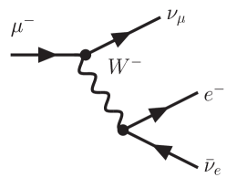
Figure 1: Muon decay: the main source of our knowledge of $g$.

The coupling constant $g$ together with the mass $M_{W}^{2}$ can be determined from the Fermi constant as measured in muon decay. The relevant corrections are known to two-loop level. The most recent calculations and earlier references can be found in Ref. [References]. The result is

$$G_{F}=\frac{g^{2}}{8M_{W}^{2}}=1.16639(1)\cdot 10^{-5}~{}\mbox{GeV}^{-2}\,.$$ (10)

The Cabibbo-Kobayashi-Maskawa matrix $V_{CKM}=\left(V_{ij}\right)$ results from diagonalizing the quark mass terms resulting from the Yukawa terms and the Higgs vacuum expectation value. It is a general unitary matrix but the phases of the quark fields can be redefined. This allows to remove 5 of the 6 phases present in a general unitary 3 by 3 matrix. The matrix $V_{CKM}$ thus contains three phases and one mixing angle. The Particle Data Group preferred parametrization is $\!{}^{{\bf?}}$

$$\left(\begin{array}[]{ccc}c_{12}c_{13}&s_{12}c_{13}&s_{13}e^{-i\delta_{13}}\\ -s_{12}c_{23}-c_{12}s_{23}s_{13}e^{i\delta_{13}}&c_{12}c_{23}-s_{12}s_{23}s_{13}e^{i\delta_{13}}&s_{23}c_{13}\\ s_{12}s_{23}-c_{12}c_{23}s_{13}e^{i\delta_{13}}&-c_{12}s_{23}-s_{12}c_{23}s_{13}e^{i\delta_{13}}&c_{23}c_{13}\,.\end{array}\right)$$ (11)

Using the measured experimental values, see below and Ref. [References],

$$s_{12}=\sin\theta_{12}\approx 0.2;\quad s_{23}\approx 0.04\quad\mbox{and}\quad s_{13}\approx 0.003$$ (12)

an approximate parametrization, known as the Wolfenstein $\!{}^{{\bf?}}$ parametrization, can be given. This is defined via

$$s_{12}c_{13}\equiv\lambda\,;\quad s_{23}c_{13}\equiv A\lambda^{2}\,;\quad\mbox{and}\quad s_{13}e^{-i\delta_{13}}\equiv A\lambda^{3}(\rho-i\eta)\,.$$ (13)

To order $\lambda^{4}$ the CKM-matrix is

$$\left(\begin{array}[]{ccc}1-\frac{\lambda^{2}}{2}&\lambda&A\lambda^{3}(\rho-i\eta)\\ -\lambda&1-\frac{\lambda^{2}}{2}&A\lambda^{2}\\ A\lambda^{3}(1-\rho-i\eta)&-A\lambda^{2}&1\end{array}\right)\,.$$ (14)

$CP$-violation is present if the phase $\delta$ is different from $0$ or $\pi$ or alternatively $\eta\neq 0$. A way to check for the presence of $CP$ violation in general set of mass matrices was found by C. Jarlskog. $\!{}^{{\bf?}}$

A main purpose of this chapter in the book is to describe how the above picture of the weak interaction and CKM mixing can be experimentally tested in the light-quark sector.

4 Semileptonic decays

A first necessary step is the determination of the parameters that occur in the Yukawa sector of the standard model. Here we concentrate on the two that can be measured directly in the light quark sector, $V_{ud}$ and $V_{us}$. As will become very clear, the strong interactions are always the main theoretical limitation on the precision determination of these quantities.

4.1 $V_{ud}$

The underlying idea always the same. The vector current has matrix-element one at zero momentum transfer because of the underlying vector Ward identities if all the quark masses involved in the vector current are equal.

The element $V_{ud}$ is measured in three main sets of decays.

• neutron: The coupling of the neutron to the weak current is given by

  $$\frac{g_{A}}{g_{V}}=-1.2670\pm 0.0035\,.$$ (15)

  where we know that $g_{V}=1$ at zero momentum transfer. In addition we use that the axial current effect is actually measurable via the angular distribution of the electron. So $\Gamma(n\to pe^{-}\bar{\nu})\sim G_{n}^{2}(1+3g_{A}^{2}/g_{V}^{2})A$
  with $A$ calculable but containing photon loops. Using the value for $g_{A}/g_{V}$ and the neutron lifetime of the 2000 particle data book $\!{}^{{\bf?}}$ and the calculations of radiative corrections quoted in Ref. [References] I obtain

  $$|V_{ud}|=0.9792(40)\,.$$ (16)

  A recent review of the situation for $|V_{ud}|$ is Ref. [References].

  At present the errors are dominated by the measurement of $g_{A}/g_{V}$. This could change in the near future.

• Nuclear superallowed $\beta$-decays: $0^{+}\to 0^{+}$

  The main advantages here are that only the vector current can contribute and that very accurate experimental results are available. The disadvantage is that the charge symmetry breaking, or isospin, effects and the photonic radiative corrections are nuclear structure dependent with an unknown error. The quoted theory errors are such that the measurements for different nuclei are in contradiction with each other. In Ref. [References] they therefore quote

  $$|V_{ud}|=0.9740(10)\,.$$ (17)

  with a substantial scale factor.

• Pion $\beta$-decay: $\pi^{+}\to\pi^{0}e^{+}\bar{\nu}$

  The theory here is very clean and improvable using CHPT.$\!{}^{{\bf?}}$ The disadvantage is that the branching ratio is about $10^{-8}$, known to about 4%. Experiments at PSI are in progress to get 0.5%.

In the future better experimental precision in neutron and $\pi$ $\beta$-decay should improve the determination since they are theoretically under better control. In any case, $|V_{ud}|$ is by far the best directly determined CKM-matrix element. The PDG averages all present measurements to

$$|V_{ud}|=0.9735(8)\,.$$ (18)

4.2 $V_{us}$

Again we use the fact that the matrix-element of a conserved vector current is one at zero momentum. But compared to the previous subsection we have additional complications:
$\bullet$ The vector current is $\bar{s}\gamma_{\mu}u$ so corrections are $(m_{s}-m_{u})^{2}$ and not $(m_{d}-m_{u})^{2}$ so they are naively larger.
$\bullet$ A longer extrapolation to the zero-momentum point is needed.
The relevant semi-leptonic decays can be measured in hyperon or in kaon decays.

Hyperon $\beta$-decays (e.g. $\Sigma^{-}\to ne^{-}\bar{\nu},\Lambda\to pe^{-}\bar{\nu}$): Here there are large theoretical problems. In CHPT the corrections are large and many new parameters show up. In addition the series does not converge too well. Curiously enough, using lowest order CHPT with model-corrections works OK. For references consult the relevant section of Ref. [References]. This area needs theoretical work very badly.

Kaon $\beta$-decays (e.g. $K^{+}\to\pi^{0}e^{+}\nu$): Both theory and data are old by now. The theory was done by Leutwyler and Roos $\!{}^{{\bf?}}$. The analysis uses old-fashioned photonic loops for the electro-magnetic corrections and one-loop CHPT for the strong corrections due to quark masses. Both aspects are at present being improved. $\!{}^{{\bf?},{\bf?}}$ The latest data are from 1987 and the most precise ones are older. There is at present a proposal at BNL while KLOE at DAPHNE should also be able to improve the precision.

The result obtained from the last process is

$$|V_{us}|=0.2196\pm 0.0023\,.$$ (19)

We can now use this to test the unitarity relation

$$|V_{us}|^{2}+|V_{ud}|^{2}=0.9959\pm 0.0019\,.$$ (20)

$|V_{ub}|^{2}$ is so small it is not visible in the precision shown here. The discrepancy is small and should be understood but there is no real cause for worry at present.

4.3 Testing CHPT/QCD and determining CHPT parameters

In the sector of semi-leptonic kaon decays CHPT unfolds all of its power. An extensive review can be found in Ref. [References] with a more recent update in Ref. [References]. There are of course also numerous model calculations and other approaches existing. An example of model calculations using Schwinger-Dyson equations is in Ref. [References]. Notice that the Schwinger-Dyson equations themselves do not constitute the model aspect but the assumptions made in their solutions.

I now simply list the main decays and which quantity they test and/or measure.

• $K\to\mu\nu$ ($K_{\ell 2}$) : Measurement of $F_{K}$. This is known to two loops $\!{}^{{\bf?}}$ in CHPT and the electromagnetic corrections have also been updated. $\!{}^{{\bf?}}$

• $K\to\pi\ell\nu$ ($K_{\ell 3}$): $V_{us}$ and form-factors, see Ref. [References] and references therein. Work on the two-loop aspects in CHPT and on the electromagnetic corrections is under way. $\!{}^{{\bf?},{\bf?}}$

• $K\to\pi\pi\ell\nu$ ($K_{\ell 4}$): Form-factors and a main source of CHPT input parameters. Known at two-loops in CHPT. $\!{}^{{\bf?}}$

• $K\to\pi\ell\nu\gamma$ ($K_{\ell 3\gamma}$): Lots of form-factors with large corrections combining to a final small correction. $\!{}^{{\bf?}}$

• $K(\pi)\to\ell\nu\gamma$ ($K(\pi)_{\ell 2\gamma}$): This has two form-factors, one normal and one anomalous. The interference between them allows to see the sign of the anomaly. This can also be done in $K_{\ell 4}$ and both confirm nicely the expectations. $\!{}^{{\bf?},{\bf?},{\bf?}}$

The situation in the semileptonic sector is generally good and we are talking about precision problems. The medium term limit on the theory here is the fact that for the quark mass effects we need many rather high order parameters in CHPT we need to determine somehow. Given the relative paucity of full higher order calculations at present not much more can be said. We can expect major progress here in the medium term.

The long term limit will probably come from the fact that the electromagnetic corrections in the weak decays have free parameters at higher orders as well. These provide both a virtual photon and a virtual $W$-boson resulting in an extremely hard problem of matching long and short distance aspects. Given the difficulty in treating the same problems with a virtual $W$ only as discussed below, it will probably take some time before this question is fully settled.

5 Non-leptonic Decays: $K\to\pi\pi$ and $K$-${\overline{K^{0}}}$ mixing

We have been rather successful in understanding the theory behind the semi-leptonic decays discussed in the previous section. Basically we always used CHPT or similar arguments to get at the coupling of the $W$-boson to hadrons, problems only occur when we want to go to very high precision. A similar simple approach fails completely for non-leptonic decays. I’ll first discuss the main qualitative problem that shows up in trying to estimate these decays, then the phenomenology involved in mixing phenomena and then proceed in the various steps needed to actually calculate these processes in the standard model.

5.1 The $\Delta I=1/2$ rule

The underlying problem appears when we try to calculate $K\to\pi\pi$ decays in a similar fashion as for the semi-leptonic decays. For $K^{+}\to\pi^{+}\pi^{0}$ we can draw two Feynman diagrams with a simple $W^{+}$ exchange as shown in Fig. 2.

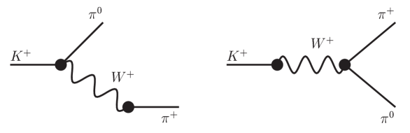
Figure 2: The two naive $W^{+}$-exchange diagrams for $K^{+}\longrightarrow\pi^{+}\pi^{0}$.

The relevant $W^{+}$-hadron couplings have all been measured in semi-leptonic decays and so we have a unique prediction. Comparing this with the measured decay we get within a factor of two or so. The approximation described here is known as naive factorization.

A much worse result appears when we try the same method for the neutral decay $K^{0}\to\pi^{0}\pi^{0}$. As shown in Fig. 3 there is no possibility to draw diagrams similar to those in Fig. 2. The needed vertices always violate charge-conservation.

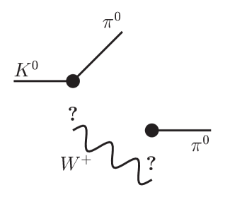
Figure 3: No simple $W^{+}$-exchange diagram is possible for $K^{0}\longrightarrow\pi^{0}\pi^{0}$.

So we expect that the neutral decay should be small compared with the ones with charged pions. Well, if we look at the experimental results we see

$$\Gamma(K^{0}\longrightarrow\pi^{0}\pi^{0})= \displaystyle\frac{1}{2}\Gamma(K_{S}\longrightarrow\pi^{0}\pi^{0}) =2.3\cdot 10^{-12}\mbox{ MeV}$$

$$\Gamma(K^{+}\longrightarrow\pi^{+}\pi^{0})= \displaystyle 1.1\cdot 10^{-14}\mbox{ MeV}$$ (21)

So the expected zero one is by far the largest !!!

The same conundrum can be expressed in terms of the isospin amplitudes: 

$$A[K^{0}\to\pi^{0}\pi^{0}] \equiv \sqrt{\frac{1}{3}}{A_{0}}-\sqrt{\frac{2}{3}}\,{A_{2}}$$

$$A[K^{0}\to\pi^{+}\pi^{-}] \equiv \sqrt{\frac{1}{3}}{A_{0}}+\sqrt{\frac{1}{6}}\,{A_{2}}$$

$$A[K^{+}\to\pi^{+}\pi^{0}] \equiv \frac{\sqrt{3}}{2}{A_{2}}\,.$$ (22)

The above quoted experimental results can now be rewritten as

$$\left|\frac{A_{0}}{A_{2}}\right|_{\mbox{exp}}=22.1$$ (23)

while the naive $W^{+}$-exchange discussed would give

$$\left|\frac{A_{0}}{A_{2}}\right|_{\mbox{naive}}=\sqrt{2}\,.$$ (24)

This discrepancy is known as the problem of the $\Delta I=1/2$ rule. The amplitude which changes the isospin $1/2$ of the kaon to the zero isospin two pion system is much larger than the one that changes the isospin to 2 by $3/2$.

Some enhancement is easy to understand from final state $\pi\pi$-rescattering. Removing these and higher order effects in the light quark masses one obtains $\!{}^{{\bf?}}$

$$\left|\frac{A_{0}}{A_{2}}\right|_{\chi}=16.4\,.$$ (25)

This changes the discrepancy somewhat but is still different by an order of magnitude from the naive result (24). The difference will have to be explained by pure strong interaction effects and it is a qualitative change, not just a quantitative one.

Later we also need the amplitudes with the final state interaction phase removed via

$$A_{I}=-ia_{I}e^{i\delta_{I}}$$ (26)

for $I=0,2$. $\delta_{I}$ is the angular momentum zero isospin I scattering phase at the kaon mass.

5.2 Phenomenology of $K$-${\overline{K^{0}}}$ mixing and CP-violation

The $K^{0}$ and ${\overline{K^{0}}}$ states are the ones with $\bar{s}d$ and $\bar{d}s$ quark content respectively. Up to free phases in these states we can define the action of $CP$ on these states as

$$CP|K^{0}\rangle=-|{\overline{K^{0}}}\rangle\,.$$ (27)

We can construct eigenstates with a definite $CP$ transformation:

$$K^{0}_{1(2)} = \frac{1}{\sqrt{2}}\left(K^{0}-(+){\overline{K^{0}}}\right)$$

$$CP|K_{1(2)} = +(-)|K_{1(2)}\,.$$ (28)

Now the main decay mode of $K^{0}$-like states is $\pi\pi$. A two pion state with charge zero in spin zero is always CP even. Therefore the decay $K_{1}\to\pi\pi$ is possible but $K_{2}\to\pi\pi$ is impossible; $K_{2}\to\pi\pi\pi$ is possible. Phase-space for the $\pi\pi$ decay is much larger than for the three-pion final state. Therefore if we start out with a pure $K^{0}$ or ${\overline{K^{0}}}$ state, the $K_{2}$ component in its wave-function lives much longer than the $K_{1}$ component. So after a, by microscopic standards, long time only the $K_{2}$ component survives. This was the solution to the two particles with the same mass and production but very different lifetimes mentioned in the historical overview, the socalled tau-theta puzzle.

In the early sixties, as you see it pays off to do precise experiments, one actually measured $\!{}^{{\bf?}}$

$$\frac{\Gamma(K_{L}\to\pi^{+}\pi^{-})}{\Gamma(K_{L}\to\mbox{all})}=(2\pm 0.4)\cdot 10^{-3}\,.$$ (29)

So we see that $CP$ is violated .

This leaves us with the questions:

• Does $K_{1}$ turn in to $K_{2}$ ($CP$-violation in mixing or indirect $CP$ violation)?

• Does $K_{2}$ decay directly into $\pi\pi$ (direct $CP$ violation)?

In fact, the answer to both is YES  and is major qualitative test of the standard model Higgs-fermion sector and the entire $CKM$-picture of $CP$-violation.

Let us now describe the $K^{0}{\overline{K^{0}}}$ system in somewhat more detail. The Hamiltonian, seen as a two state system, is given by

$$i\frac{d}{dt}\left(\begin{array}[]{c}K^{0}\\[2.84526pt] {\overline{K^{0}}}\end{array}\right)=\left(\begin{array}[]{cc}M_{11}-\frac{i}{2}\Gamma_{11}&M_{12}-\frac{i}{2}\Gamma_{12}\\[2.84526pt] M_{21}-\frac{i}{2}\Gamma_{21}&M_{22}-\frac{i}{2}\Gamma_{22}\end{array}\right)\left(\begin{array}[]{c}K^{0}\\[2.84526pt] {\overline{K^{0}}}\end{array}\right)$$ (30)

where $M=\left(M_{ij}\right)$ and $\Gamma=\left(\Gamma_{ij}\right)$ are hermitian two by two matrices. The Hamiltonian itself is allowed to have a non-hermitian part since we do not conserve probability here. The kaons themselves can decay and the anti-hermitian part $\Gamma$ describes the decays of the kaons to the “rest of the universe.”

CPT implies, a derivation can be found in Ref. [References],

$$M_{11}=M_{22}\quad \Gamma_{11}=\Gamma_{22}$$

$$M_{12}=M_{21}^{*}\quad \Gamma_{12}=\Gamma_{21}^{*}$$ (31)

and this assumption can in fact be relaxed for tests of CPT.

Diagonalizing the Hamiltonian we obtain

$$K_{S(L)}=\frac{1}{\sqrt{1+|\tilde{\varepsilon}|^{2}}}\left(K_{1(2)}+\tilde{\varepsilon}K_{2(1)}\right)$$ (32)

as physical propagating states. Notice that they are not orthogonal, which is allowed since the Hamiltonian is not hermitian.

We define the following observables

$$\eta_{+-} \equiv \frac{A(K_{L}\to\pi^{+}\pi^{-})}{A(K_{S}\to\pi^{+}\pi^{-})}\,,$$

$$\eta_{00} \equiv \frac{A(K_{L}\to\pi^{0}\pi^{0})}{A(K_{S}\to\pi^{0}\pi^{0})}\,,$$

$$\varepsilon \equiv \frac{A(K_{L}\to(\pi\pi)_{I=0})}{A(K_{S}\to(\pi\pi)_{I=0})}$$ (33)

and

$$\varepsilon^{\prime}=\frac{1}{\sqrt{2}}\left(\frac{A(K_{L}\to(\pi\pi)_{I=2})}{A(K_{S}\to(\pi\pi)_{I=0})}-\varepsilon\frac{A(K_{S}\to(\pi\pi)_{I=2})}{A(K_{S}\to(\pi\pi)_{I=0})}\right)\,.$$ (34)

The latter has been specifically constructed to remove the $K^{0}$-${\overline{K^{0}}}$ transition. $|\varepsilon|$, $|\eta_{+-}|$ and $|\eta_{00}|$ are directly measurable as ratios of decay rates.

We now make a series of approximations that are experimentally valid,

$$|\mbox{Im}a_{0}|,|\mbox{Im}a_{2}| << |\mbox{Re}a_{2}|<<|\mbox{Re}a_{0}|$$

$$|\varepsilon|,|\tilde{\varepsilon}| << 1$$

$$\quad|\varepsilon^{\prime}| << |\varepsilon|\,,$$ (35)

to obtain the usually quoted expressions

$$\varepsilon^{\prime}=\frac{i}{\sqrt{2}}e^{i(\delta_{2}-\delta_{0})}\frac{\mbox{Re}a_{2}}{\mbox{Re}a_{0}}\left(\frac{\mbox{Im}a_{2}}{\mbox{Re}a_{2}}-\frac{\mbox{Im}a_{0}}{\mbox{Re}a_{0}}\right)$$ (36)

and

$$\varepsilon=\tilde{\varepsilon}+i\frac{\mbox{Im}a_{0}}{\mbox{Re}a_{0}}\,.$$ (37)

For the latter we use $\Delta m=m_{L}-m_{S}\approx\frac{\Delta\Gamma}{2}$ and $\Gamma_{L}<<\Gamma_{S}$ and the fact that $\Gamma_{12}$ is dominated by $\pi\pi$ states and get

$$\varepsilon=\frac{1}{\sqrt{2}}e^{i\pi/4}\left(\frac{\mbox{Im}M_{12}}{\Delta m}+\frac{\mbox{Im}a_{0}}{\mbox{Re}a_{0}}\right)\,.$$ (38)

Putting all the above together we finally get to

$$\eta_{+-}=\varepsilon+\varepsilon^{\prime}\quad\mbox{and}\quad\eta_{00}=\varepsilon-2\varepsilon^{\prime}$$

Where you can see that $\varepsilon$ describes the indirect part and $\varepsilon^{\prime}$ the direct part, since the mixing contribution would be the same for $\eta_{+-}$ and $\eta_{00}$.

The real part of $\tilde{\varepsilon}$ can be measured in semi-leptonic decays via the ratio

$$\delta=\frac{\displaystyle\Gamma(K_{L}\to\pi^{-}\ell^{+}\nu_{\ell})-\Gamma(K_{L}\to\pi^{+}\ell^{-}\bar{\nu}_{\ell})}{\displaystyle\Gamma(K_{L}\to\pi^{-}\ell^{+}\nu_{\ell})+\Gamma(K_{L}\to\pi^{+}\ell^{-}\bar{\nu}_{\ell})}\,.$$ (39)

The latter relation assumes the $\Delta S=\Delta Q$ rule which is satisfied to a very good precision in the Standard Model. The sign of the lepton charge thus tells us whether $K_{L}$ decayed as a $K^{0}$ or a ${\overline{K^{0}}}$.

5.3 Experimental results

Experimentally, $\!{}^{{\bf?},{\bf?}}$

$$2\,\mbox{Re}\varepsilon\approx\delta=0.00331\pm 0.00006\,.$$ (40)

including the recent preliminary KTeV result.

$\varepsilon$ is well known. $\!{}^{{\bf?}}$

$$|\varepsilon|=(2.271\pm 0.017)\cdot 10^{-3}\,,$$ (41)

as determined by several high precision experiments which are in good agreement with each other.

The experimental situation on ${\varepsilon^{\prime}/\varepsilon}$ was unclear for a long time. Two large experiments, NA31 at CERN and E731 at FNAL, obtained conflicting results in the mid 1980’s. Both groups have since gone on and build improved versions of their detectors, NA48 at CERN and KTeV at FNAL. ${\varepsilon^{\prime}/\varepsilon}$ is measured via the double ratio

$$\mbox{Re}\left(\frac{\varepsilon^{\prime}}{\varepsilon}\right) = \frac{1}{6}\left\{1-\left|\frac{\eta_{00}}{\eta_{+-}}\right|^{2}\right\}$$ (42)

$$= \frac{1}{6}\left\{1-\frac{\displaystyle\Gamma(K_{L}\to\pi^{+}\pi^{-})/\Gamma(K_{S}\to\pi^{+}\pi^{-})}{\displaystyle\Gamma(K_{L}\to\pi^{0}\pi^{0})/\Gamma(K_{S}\to\pi^{0}\pi^{0})}\right\}\,.$$

The two main experiments follow a somewhat different strategy in measuring this double ratio, mainly in the way the relative normalization of $K_{L}$ and $K_{S}$ components is treated. After some initial disagreement with the first results, KTeV has reanalyzed their systematic errors and the situation for ${\varepsilon^{\prime}/\varepsilon}$ is now quite clear. We show the recent results in Table 1. The data are taken from Ref. [References] and the recent reviews in the Lepton-Photon conference. $\!{}^{{\bf?},{\bf?}}$

NA31	$(23.0\pm 6.5)\times 10^{-4}$
E731	$(7.4\pm 5.9)\times 10^{-4}$
KTeV 96	$(23.2\pm 4.4)\times 10^{-4}$
KTeV 97	$(19.8\pm 2.9)\times 10^{-4}$
NA48 97	$(18.5\pm 7.3)\times 10^{-4}$
NA48 98+99	$(15.0\pm 2.7)\times 10^{-4}$
ALL	$(17.2\pm 1.8)\times 10^{-4}$

Table 1: Recent results on $\varepsilon^{\prime}/\varepsilon$. The years refer to the data sets.

5.4 Standard Model Diagrams

The weak nonleptonic decays all happen via the exchange of a $W$-boson. The main diagram is depicted in Fig. 4 where we have only indicated one possible routing of the quark legs and no extra gluons. This figure should be understood as an indication of the type of diagrams responsible. The contribution depicted here is sometimes referred to as the spectator contribution, but that name normally implies some more approximations. The other simple $W$-exchange diagram is similarly known as the annihilation contribution and is depicted in Fig. 5.

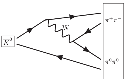
Figure 4: The $W$-exchange diagram, sometimes referred to as the spectator mechanism. Extra gluons etc. are not shown.

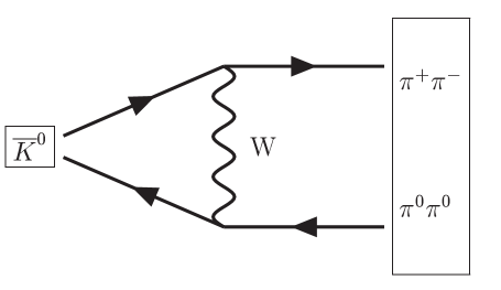
Figure 5: The $W$-exchange diagram, sometimes referred to as the annihilation mechanism. Extra gluons etc. are not shown.

These diagrams, and the ones with extra gluons and light quarks, are the ones responsible for the main part of the decay rate.

$CP$-violation with the CKM mechanism goes via another class of diagrams. The complex phase in the CKM matrix can be removed as soon as effectively not all three of the generations contribute. The diagrams thus need to have a component in it that involves all three generations in order to contribute to $CP$-violation. The set of diagrams, depicted schematically in Fig. 6, responsible for $K^{0}{\overline{K^{0}}}$ mixing are known as box diagrams. It is the presence of the virtual intermediate quark lines of up, charm and top quarks that produces the $CP$-violation.

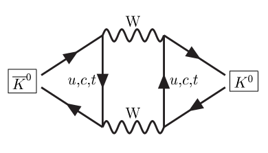
Figure 6: The box diagram contribution to $K^{0}{\overline{K^{0}}}$ mixing. Crossed versions and diagrams with extra gluons etc. are not shown.

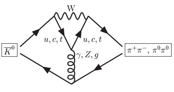
Figure 7: The Penguin diagram contribution to $K\to\pi\pi$. Extra gluons and crossed versions etc. are not shown.

The Penguin diagram shown in Fig. 7 contributes to the direct $CP$-violation as given by $\varepsilon^{\prime}$. Again, $W$-couplings to all three generations show up so CP-violation is possible in $K\to\pi\pi$. This is a qualitative prediction of the standard model and borne out by experiment. The main problem is now to embed these diagrams and the simple $W$-exchange in the full strong interaction. The $\Delta I=1/2$ rule shows that there will have to be large corrections to the naive picture.

5.5 The first QCD correction

The naive factorization approach we described earlier can reformulated in a different fashion which makes it easier to generalize later on. Since the kaon mass is so much lower than the $W$ mass, we expect that at first approximation we can neglect the momentum dependence of the $W$-propagator. So we replace the effect of $W$ exchange of Figs. 4 and 5 by the effect of a local four-quark operator. So we replace at the quark level Fig. 8 by the operators depicted in Fig. 9.

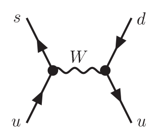
Figure 8: The $W$-exchange depicted at the quark level.

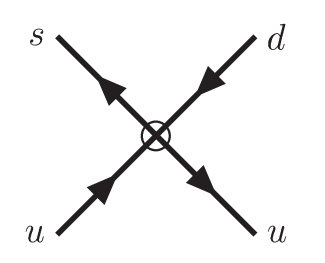
Figure 9: The effect of the local operators depicted at the quark level.

The $W$ exchange at tree level can be described by the effective Hamiltonian

$${\cal H}_{\mbox{eff}}^{\mbox{tree}}=\sum_{i}C_{i}(\mu)Q_{i}(\mu)\displaystyle{\cal H}_{\mbox{eff}}=\frac{G_{F}}{\sqrt{2}}V_{ud}V_{us}^{*}\sum_{i}z_{i}Q_{i}^{u}\,.$$ (43)

The coefficients $z_{i}$ are real and the CKM-matrix elements occurring are shown explicitly. The four-quark operators $Q_{i}^{u}$ are defined by

$$Q_{1}^{u} = (\bar{s}_{\alpha}\gamma_{\mu}u_{\beta})_{L}(\bar{u}_{\beta}\gamma^{\mu}d_{\alpha})_{L}\,,$$

$$Q_{2}^{u} = (\bar{s}_{\alpha}\gamma_{\mu}u_{\alpha})_{L}(\bar{u}_{\beta}\gamma^{\mu}d_{\beta})_{L}\,,$$ (44)

with $(\bar{q}\gamma_{\mu}q^{\prime})_{L}=\bar{q}\gamma_{\mu}(1-\gamma_{5})q^{\prime}$. In order to have the same matrix elements as $W$-exchange at tree level up to terms of order $m_{K}^{2}/m_{W}^{2}$ we need to set

$$z_{1}=0\quad\mbox{and}\quad z_{2}=1\,.$$ (45)

The effect of gluonic interactions can now be taken into account. Diagrams like the one depicted in Fig. 10 contribute as well.

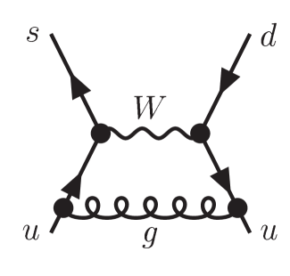
Figure 10: A diagram with a gluonic correction to tree level $W$-exchange.

The total results is finite, after the renormalization of $\alpha_{S}$ is duly taken into account. The result, again up to terms of order $m_{K}^{2}/m_{W}^{2}$, can be taken into account by replacing $z_{1}$ and $z_{2}$ by

$$z_{1} = -\frac{\alpha_{S}}{4\pi}3\ln\left(\frac{m_{W}^{2}}{\mu^{2}}\right)\approx 0.84\,,$$

$$z_{2} = 1+\frac{\alpha_{S}}{4\pi}\ln\left(\frac{m_{W}^{2}}{\mu^{2}}\right)\approx 1.28\,.$$ (46)

For the numerical results we have used $\mu\approx 1~{}$GeV and $\alpha_{S}\approx 0.4$.

What conclusions can we draw from this? First of all, the corrections are rather large because of the presence of the large logarithmic term. This we will have to take care of more accurately as described below. A second consequence is that we have already gone some way towards solving the $\Delta I=1/2$ rule. The operators

$$Q_{\pm}=\frac{1}{2}\left(Q_{2}^{u}\pm Q_{1}^{u}\right)$$ (47)

have a different isospin behaviour. $Q_{-}$ is pure isospin $1/2$ while $Q_{+}$ has both isospin $1/2$ and $3/2$ components. The tree level result gave both of them with coefficients $z_{\pm}=1$ while Eq. (5.5) gives

$$z_{-}\approx 2.1\quad\mbox{and}\quad z_{+}\approx 0.44\,.$$ (48)

We see a significant enhancement of the $\Delta I=1/2$ component and a suppression of the $\Delta I=3/2$ component. We have not said how one gets from the quark level to the meson level here. This will be discussed in more detail in Sect. 6.

5.6 The steps from quarks to mesons in the weak interaction

We need to extend the calculation of Sect. 5.5 in several ways. We only took into account the simplest gluonic diagrams, we should preferably go to higher orders and the large logarithms need to be treated to all orders if possible. The latter can be done since the large logarithms contain the subtraction scale $\mu$. The dependence on $\mu$ of an observable must vanish, which means that coefficients of the type $z_{i}$ must depend on $\mu$ in such a way that when a matrix element between physical states is taken the $\mu$-dependence cancels. This can be used to calculate the variation of the $z_{i}$ with $\mu$ in a way which includes all term of order $\left(\alpha_{S}\ln\mu^{2}\right)^{n}$ with a one-loop calculation and the techniques of the renormalization group. It can also be improved by going to higher orders. We proceed thus in several steps, we replace the exchange of $W$’s by a series of operators at a scale $\mu$ such that the logarithms of the type $\ln(m_{W}^{2}/\mu^{2})$ are small. The coefficients $z_{i}$ (or more general $C_{i}$) are universal and can be calculated by comparing matrix elements of $W$-exchange with the matrix elements of the local operators. This correspondence is independent of the choice of matrix elements, so the external states can be chosen to minimize the effort needed for the calculation.

The $\mu$ dependence of the $C_{i}$ is then exploited via the renormalization group to resum all large logarithms to the order desired, or rather to the order the calculations can be practically performed. The last step is then to take the matrix elements of the operators at a low scale $\mu$ which should avoid large logarithms of the type $\ln(m_{K}^{2}/\mu^{2})$.

The three steps of the full calculation are depicted in Fig. 11.

ENERGY SCALE	FIELDS	Effective Theory
$M_{W}$	$W,Z,\gamma,g$; $\tau,\mu,e,\nu_{\ell}$; $t,b,c,s,u,d$	Standard Model
	$\Downarrow$ using OPE
$\lesssim m_{c}$	$\gamma,g$; $\mu,e,\nu_{\ell}$; $s,d,u$	QCD,QED, ${\cal H}_{\mbox{eff}}^{|\Delta S|=1,2}$
	$\Downarrow$ ???
$M_{K}$	$\gamma$; $\mu,e,\nu_{\ell}$; $\pi$, $K$, $\eta$	CHPT

Figure 11: A schematic exposition of the various steps in the calculation of nonleptonic matrix-elements.

First we integrated out the heaviest particles step by step using Operator Product Expansion methods. The steps OPE we describe in the next subsections while step ??? we will split up in more subparts later.

5.7 Step I: from SM to OPE

The first step for the processes we discuss in this review concerns the standard model diagrams of Fig. 12.

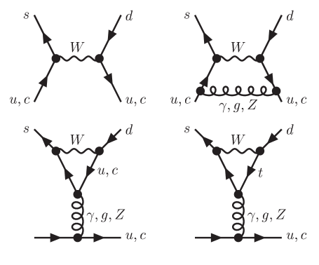
Figure 12: The standard model diagrams to be calculated at a high scale.

We replace their effect with a contribution of an effective Hamiltonian given by

$${\cal H}_{\mbox{eff}} = \sum_{i}C_{i}(\mu)Q_{i}(\mu)$$ (49)

$$= \frac{G_{F}}{\sqrt{2}}V_{ud}V_{us}^{*}\sum_{i}\left(z_{i}-y_{i}\frac{V_{td}V_{ts}^{*}}{V_{ud}V_{us}^{*}}\right)Q_{i}\,.$$

In the last part we have real coefficients $z_{i}$ and $y_{i}$ and the CKM-matrix elements occurring are shown explicitly. The four-quark operators $Q_{i}$ are defined by

$$Q_{1,2} = Q_{1,2}^{u}-Q_{1,2}^{c}\,,$$

$$Q_{1}^{u} = (\bar{s}_{\alpha}\gamma_{\mu}u_{\beta})_{L}(\bar{u}_{\beta}\gamma^{\mu}d_{\alpha})_{L}\,,$$

$$Q_{1}^{c} = (\bar{s}_{\alpha}\gamma_{\mu}c_{\beta})_{L}(\bar{c}_{\beta}\gamma^{\mu}d_{\alpha})_{L}\,,$$

$$Q_{2}^{u} = (\bar{s}_{\alpha}\gamma_{\mu}u_{\alpha})_{L}(\bar{u}_{\beta}\gamma^{\mu}d_{\beta})_{L}\,,$$

$$Q_{2}^{c} = (\bar{s}_{\alpha}\gamma_{\mu}c_{\alpha})_{L}(\bar{c}_{\beta}\gamma^{\mu}d_{\beta})_{L}\,,$$

$$Q_{3} = (\bar{s}_{\alpha}\gamma_{\mu}d_{\alpha})_{L}\sum_{q=u,d,s,c,b}(\bar{q}_{\beta}\gamma^{\mu}q_{\beta})_{L}\,,$$

$$Q_{4} = (\bar{s}_{\alpha}\gamma_{\mu}d_{\beta})_{L}\sum_{q=u,d,s,c,b}(\bar{q}_{\beta}\gamma^{\mu}q_{\alpha})_{L}\,,$$

$$Q_{5} = (\bar{s}_{\alpha}\gamma_{\mu}d_{\alpha})_{L}\sum_{q=u,d,s,c,b}(\bar{q}_{\beta}\gamma^{\mu}q_{\beta})_{R}\,,$$

$$Q_{6} = (\bar{s}_{\alpha}\gamma_{\mu}d_{\beta})_{L}\sum_{q=u,d,s,c,b}(\bar{q}_{\beta}\gamma^{\mu}q_{\alpha})_{R}\,,$$

$$Q_{7} = (\bar{s}_{\alpha}\gamma_{\mu}d_{\alpha})_{L}\sum_{q=u,d,s,c,b}\frac{3}{2}e_{q}(\bar{q}_{\beta}\gamma^{\mu}q_{\beta})_{R}\,,$$

$$Q_{8} = (\bar{s}_{\alpha}\gamma_{\mu}d_{\beta})_{L}\sum_{q=u,d,s,c,b}\frac{3}{2}e_{q}(\bar{q}_{\beta}\gamma^{\mu}q_{\alpha})_{R}\,$$

$$Q_{9} = (\bar{s}_{\alpha}\gamma_{\mu}d_{\alpha})_{L}\sum_{q=u,d,s,c,b}\frac{3}{2}e_{q}(\bar{q}_{\beta}\gamma^{\mu}q_{\beta})_{L}\,,$$

$$Q_{10} = (\bar{s}_{\alpha}\gamma_{\mu}d_{\beta})_{L}\sum_{q=u,d,s,c,b}\frac{3}{2}e_{q}(\bar{q}_{\beta}\gamma^{\mu}q_{\alpha})_{L}$$ (50)

with $(\bar{q}\gamma_{\mu}q^{\prime})_{(L,R)}=\bar{q}\gamma_{\mu}(1\mp\gamma_{5})q^{\prime}$; $\alpha$ and $\beta$ are colour indices.

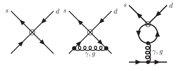
Figure 13: The diagrams needed for the matrix-elements calculated at a scale $\mu_{H}\approx m_{W}$ using the effective Hamiltonian.

We calculate now matrix elements between quarks and gluons in the standard model using the diagrams of Fig. 12 and equate those to the same matrix-elements calculated using the effective Hamiltonian of Eq. (49) and the diagrams of Fig. 13. This determines the value of the $z_{i}$ and $y_{i}$. The top quark and the $W$ and $Z$ bosons are integrated out all at the same time. There should be no large logarithms present due to that. The scale $\mu=\mu_{H}$ in the diagrams of Fig. 13 of the OPE expansion diagrams should be chosen of the order of the $W$ mass. The scale $\mu_{W}$ in the Standard Model diagrams of Fig. 12 should be chosen of the same order.

Notes:
$\bullet$ In the Penguin diagrams $CP$-violation shows up since all 3 generations are present.
$\bullet$ The equivalence is done by calculating matrix-elements between Quarks and Gluons
$\bullet$ The SM part is $\mu_{W}$-independent to $\alpha_{S}^{2}(\mu_{W})$.
$\bullet$ OPE part: The $\mu_{H}$ dependence of $C_{i}(\mu_{H})$ cancels the $\mu_{H}$ dependence of the diagrams to order $\alpha_{S}^{2}(\mu_{H})$.

This procedure gives at $\mu_{W}=\mu_{H}=M_{W}$ in the NDR-scheme  the numerical values given in Table 2.

$z_{1}$	0.053	$g,\gamma$-box
$z_{2}$	0.981	$W^{+}$-exchange $g,\gamma$-box
$y_{3}$	0.0014	$g,Z$-Penguin $WW$-box
$y_{4}$	$-$0.0019	$g$-Penguin
$y_{5}$	0.0006	$g$-Penguin
$y_{6}$	$-$0.0019	$g$-Penguin
$y_{7}$	0.0009	$\gamma,Z$-Penguin
$y_{8}$	0.
$y_{9}$	$-$0.0074	$\gamma,Z$-Penguin $WW$-box
$y_{10}$	0.

Table 2: The Wilson coefficients and their main source at the scale $\mu_{H}=m_{W}$ in the NDR-scheme.

In the same table I have given the main source of these numbers. Pure tree-level $W$-exchange would have only given $z_{2}=1$ and all others zero. Note that the coefficients from $\gamma,Z$ exchange are similar to the gluon exchange ones since $\alpha_{S}$ at this scale is not very big.

5.8 Step II

Now comes the main advantage of the OPE formalism. Using the renormalization group equations we can calculate the change with $\mu$ of the $C_{i}$ thus resumming the $\log\left(m_{W}^{2}/\mu^{2}\right)$ effects.

The renormalization group equation (RGE) for the strong coupling is

$$\mu\frac{d}{d\mu}g_{S}(\mu)=\beta(g_{S}(\mu))$$ (51)

and for the Wilson coefficients

$$\mu\frac{d}{d\mu}C_{i}(\mu)=\gamma_{ji}(g_{S}(\mu),\alpha)C_{j}(\mu)\,.$$ (52)

$\beta$ is the QCD beta function for the running coupling.

The coefficients $\gamma_{ij}$ are the elements of the anomalous dimension matrix $\hat{\gamma}$. This can be derived from the infinite parts of loop diagrams and this has been done to one $\!{}^{{\bf?}}$ and two loops.$\!{}^{{\bf?}}$ The series in $\alpha$ and $\alpha_{S}$ is known to

$$\hat{\gamma}=\hat{\gamma}^{0}_{S}\frac{\alpha_{S}}{4\pi}+\hat{\gamma}^{1}_{S}\left(\frac{\alpha_{S}}{4\pi}\right)^{2}+\hat{\gamma}_{e}\frac{\alpha}{4\pi}+\hat{\gamma}_{se}\frac{\alpha_{S}}{4\pi}\frac{\alpha}{4\pi}+\cdots$$ (53)

Many subtleties are involved in this calculation.$\!{}^{{\bf?},{\bf?}}$ They all are related to the fact that everything at higher loop orders need to be specified correctly, and many things which are equal at tree level are no longer so in $d\neq 4$ and at higher loops. The main subtleties are:
$\bullet$ The definition of $\gamma_{5}$ is important: Naive dimensional regularization (NDR), $\gamma_{5}$ anticommutes with $\gamma_{\mu}$, versus ’t Hooft-Veltman (HV), $\gamma_{5}$ anticommutes with the 4-dimensional part of $\gamma_{\mu}$ but commutes with the $d-4$-dimensional part.
$\bullet$ Fierzing is important: special care needs to be taken how to write the operators
$\bullet$ Evanescent operators
$\bullet$ The definition of the axial current. The NDR one is conserved for massless quarks but the HV one has an ambiguity since $\{\gamma_{\mu},\gamma_{5}\}\neq 0$.

An introductory review to this is Ref. [References] and a review with numerical results for all the Wilson coefficients is Ref. [References]. The analytical solution of the equations (52) to two-loop order is somewhat tricky as described in the quoted references. The numbers below are obtained by numerically integrating Eq. (52).

We need to perform the following steps to get down to a scale $\mu_{OPE}$ somewhere around 1 GeV. Starting from the values of $z_{i}$ and $y_{i}$ given in Table 2 at the scale $\mu_{H}$.

1. Solve Eqs. (52) numerically and/or analytically; run from ${\mu_{H}}$ to ${\mu_{b}}$

2. At $\mu_{b}$$\approx m_{b}$ remove $b$-quark and do matching to theory without $b$. This is done by calculating matrix elements of the effective Hamiltonian in the five quark picture and in the four quark picture and putting them equal. This does lead to discontinuities in the values of the $C_{i}$.

3. run down from $\mu_{b}$ to $\mu_{c}$$\approx m_{c}$

4. At $\mu_{c}$ remove the $c$-quark and do matching to the theory without $c$.

5. run from $\mu_{c}$ to $\mu_{\mbox{OPE}}$

This way we summed all large logarithms including $m_{W}$, $m_{Z}$, $m_{t}$, $m_{b}$ and $m_{c}$. This is easily done this way, impossible otherwise.

Notice that we had lots of scales $\mu_{i}$. In principle nothing depends on any of them and varying them gives an indication of the neglected higher order corrections.

With the inputs $m_{t}(m_{t})=166~{}GeV$, $\alpha=1/137.0$, $\alpha_{S}(m_{Z})=0.1186$ which led to the initial conditions shown in table 2, we can perform the above procedure down to $\mu_{OPE}$. Results for 900 MeV are shown in columns two and three of Table 3.

i	$z_{i}$	$y_{i}$	$z_{i}$	$y_{i}$
	$\mu_{OPE}=0.9$ GeV		$\mu_{X}=0.9$ GeV
$z_{1}$	$-$0.490	0.	$-$0.788	0.
$z_{2}$	1.266	0.	1.457	0.
$z_{3}$	0.0092	0.0287	0.0086	0.0399
$z_{4}$	$-$0.0265	$-$0.0532	$-$0.0101	$-$0.0572
$z_{5}$	0.0065	0.0018	0.0029	0.0112
$z_{6}$	$-$0.0270	$-$0.0995	$-$0.0149	$-$0.1223
$z_{7}$	2.6$~{}10^{-5}$	$-$0.9$~{}10^{-5}$	0.0002	$-$0.00016
$z_{8}$	5.3$~{}10^{-5}$	0.0013	6.8$~{}10^{-5}$	0.0018
$z_{9}$	5.3$~{}10^{-5}$	$-$0.0105	0.0003	$-$0.0121
$z_{10}$	$-$3.6$~{}10^{-5}$	0.0041	$-$8.7$~{}10^{-5}$	0.0065

Table 3: The Wilson coefficients $z_{i}$ and $y_{i}$ at a scale $\mu_{\mbox{OPE}}=$ 900 MeV in the NDR scheme and in the $X$-boson scheme at $\mu_{X}=$ 900 MeV.

Notice that $z_{1}$ and $z_{2}$ have changed much from $0$ and $1$ and are also significantly different from the simple one-loop estimate. This is the short-distance contribution to the $\Delta I=1/2$ rule. We also see a large enhancement of $y_{6}$ and $y_{8}$, which will lead to our value of $\varepsilon^{\prime}$.

A similar exercise can be performed for $K^{0}$-${\overline{K^{0}}}$ mixing.$\!{}^{{\bf?}}$ This yields the effective Hamiltonian

$${\cal H}_{\mbox{eff}}^{\Delta S=2}=C_{\Delta S=2}\left(\bar{s}_{\alpha}\gamma_{\mu}d_{\alpha}\right)_{L}\left(\bar{s}_{\beta}\gamma_{\mu}d_{\beta}\right)_{L}$$ (54)

with

$$C_{\Delta S=2} = \frac{G_{F}^{2}M_{W}^{2}}{16\pi^{2}}\left[\lambda_{c}^{2}\eta_{1}S_{0}(x_{c})+\lambda_{t}^{2}\eta_{2}S_{0}(x_{t})+2\lambda_{c}\lambda_{t}S_{0}(x_{c},x_{t})\right]$$ (55)

$$\times\alpha_{S}^{(-2/9)}(\mu)\left(1+\frac{\alpha_{S}(\mu)}{4\pi}J_{3}\right)$$

and

$$x_{c}=\frac{m_{c}}{M_{W}^{2}}\quad x_{t}=\frac{m_{t}}{M_{W}^{2}}\quad\lambda_{i}=-V_{id}V_{is}^{*}\quad J_{3}(n_{f}=3)=\frac{307}{162}\,.$$ (56)

The functions were first derived by Inami and Lin $\!{}^{{\bf?}}$

$$S_{0}(x_{c}) \approx x_{c}\,,$$

$$S_{0}(x_{t}) = \frac{4x_{t}-11x_{t}^{2}+x_{t}^{3}}{4(1-x_{t})^{2}}-\frac{3x_{t}^{3}\ln x_{t}}{2(1-x_{t})^{3}}\,,$$

$$S_{0}(x_{c}.x_{t}) = x_{c}\left[\ln\frac{x_{c}}{x_{t}}-\frac{3x_{t}}{4(1-x_{t})}-\frac{3x_{t}^{2}\ln x_{t}}{4(1-x_{t})^{2}}\right]\,,$$ (57)

With the same input as before, one obtains $\!{}^{{\bf?}}$

$$\quad\eta_{1}=1.53\quad\eta_{2}=0.57\quad\eta_{3}=0.47\,.$$ (58)

5.9 Step III: Matrix elements

Now remember that the $C_{i}$ depend on $\mu_{OPE}$ and on the definition of the $Q_{i}$ and the numerical change in the coefficients due to the various choices possible is not negligible. It is therefore important both from the phenomenological and fundamental point of view that this dependence is correctly accounted for in the evaluation of the matrix elements. We can solve this in various ways.

• Stay in QCD $\Rightarrow$ Lattice calculations.

• QCD Sum Rules This is using the method of Ref. [References] as reviewed in these books by Colangelo and Khodjamirian.$\!{}^{{\bf?}}$

• Give up $\Rightarrow$ Naive factorization.

• Improved factorization

• $X$-boson method (or fictitious boson method)

• Large $N_{c}$ (in combination with something like the $X$-boson method.) Here the difference is mainly in the treatment of the low-energy hadronic physics. Three main approaches exist of increasing sophistication.

  • CHPT: As originally proposed by Bardeen-Buras-Gérard $\!{}^{{\bf?}}$ and now pursued mainly by Hambye and collaborators.$\!{}^{{\bf?}}$

  • ENJL (or extended Nambu-Jona-Lasinio model $\!{}^{{\bf?}}$): As mainly done by myself and J. Prades.$\!{}^{{\bf?},{\bf?},{\bf?},{\bf?},{\bf?}}$

  • LMD or lowest meson dominance approach.$\!{}^{{\bf?}}$ These papers stay with dimensional regularization throughout. The $X$-boson corrections discussed below, show up here as part of the QCD corrections.

• Dispersive methods Some matrix elements can in principle be deduced from experimental spectral functions.

Notice that there other approaches as well, e.g. the chiral quark model.$\!{}^{{\bf?},{\bf?},{\bf?}}$ These have no underlying arguments why the $\mu$-dependence should cancel, but as mentioned below, the importance of some effects was first discussed in this context. I will also not treat the calculations done using bag models and potential models which similarly do not address the $\mu$-dependence issue.

6 The Matrix elements: $X$-boson and other approaches

In this section I discuss the approaches summarized in Sect. 5.9. First I discuss the various approaches mainly in the framework of $B_{K}$ and will later quote some results for the other quantities as well, concentrating on the more recent analytical methods with an emphasis on the work I have been involved in myself.

6.1 Factorization and/or vacuum-insertion-approximation

This is quite similar to the naive estimate for $K\to\pi\pi$ described above except it is applied to the four-quark operator rather than to pure $W$-exchange. So we use

$$\langle 0|\bar{s}_{\alpha}\gamma_{\mu}d_{\alpha}|K^{0}\rangle=i\sqrt{2}F_{K}p_{K}$$ (59)

to get

$$\langle\overline{K}^{0}|{\cal H}_{eff}|K^{0}\rangle=C_{\Delta S=2}(\mu)\frac{16}{3}F_{K}^{2}m_{K}^{2}\,.$$ (60)

Now the other results are usually quoted in terms of this one, the ratio is the so-called bag-parameter  $\hat{B}_{K}$.

So vacuum-insertion or factorization yields

$$\left.\hat{B}_{K}\right|_{\mbox{\small factorization}}\equiv 1\,.$$ (61)

Using large $N_{c}$, the part where the quarks of one $K^{0}$ come from two different currents in ${\cal H}_{\mbox{eff}}$ has to be excluded yields

$$\left.\hat{B}_{K}\right|_{\mbox{\small large $N_{c}$}}\equiv 3/4\,.$$ (62)

6.2 Lattice Calculations

There are many difficulties associated with this approach at present. Recent reviews are in Ref. [References] where further references can be found. A major breakthrough was realized in Ref. [References] where the problem of the contamination by other states than the wanted $\pi\pi$ final state at the kaon $\!{}^{{\bf?}}$ mass was solved.

6.3 Sum Rule Calculations

The method of sum rules have been used in several ways. One can use the simple method of calculating spectral functions in the presence of the weak interactions. This approach has been used by many authors to calculate $B_{K}$. The original calculation is Ref. [References]. Some others are Ref. [References] These sum rules share the problem of a correct chiral limit behaviour with many other sum rules that attempt to predict properties of the pseudoscalars. In the case of $K\to\pi\pi$ decays the situation is even more difficult. The underlying three point Green function with one extra insertion of the weak operator is calculable in perturbative QCD but the problem is that it is very difficult to extract the matrix elements from sum rules here. The socalled $\!{}^{{\bf?}}$ phenomenological part of the sum rule contains contributions from many intermediate states and there is no dominance of the part where all three external legs are resonances.

This problem prompted a search for two-point sum rules that could be used to determine the matrix elements. The approach developed by Pich, de Rafael and collaborators $\!{}^{{\bf?}}$ was to calculate the spectral function of the effective Hamiltonian directly which should then be matched onto the correct chiral form for the effective Hamiltonian at low energies on the phenomenological side using a chirally correct form of resonance saturation. This approach seemed to reproduce nicely the $K\to 3\pi$ $\Delta I=3/2$ amplitude but gave a rather low value for $B_{K}$ and could not reproduce the $\Delta I=1/2$ part of the amplitude. The reason for the latter was found in Ref. [References], the octet part of the sum rule turned out to have very large QCD corrections. The reason for the low value of $B_{K}$ compared to other approaches was uncovered in Ref. [References]. Away from the chiral limit, there are low-energy operators that contribute to the sum rule but not to the wanted matrix element.

6.4 Improved Factorization

This corresponds to first taking a matrix-element between a particular quark and gluon external state of ${\cal H}_{\mbox{eff}}$. This removes the scheme and scale dependence but introduces a dependence on the particular quark external state chosen. This can be found in the paper by Buras, Jamin and Weisz quoted in Ref. [References] and has been extensively used by H.-Y. Cheng.$\!{}^{{\bf?}}$ This yields a correction factor of

$$\left(1+r_{1}\frac{\alpha_{S}(\mu)}{\pi}\right)\quad r_{1}=-\frac{7}{6}$$ (63)

for $B_{K}$ and a 10 by 10 correction matrix for the $\Delta S=1$ case taking the place of $r_{1}$ in Eq. (63).

6.5 The $X$-boson method: a simpler case first.

Let us look at the simpler example of the electromagnetic contribution to $m_{\pi^{+}}^{2}-m_{\pi^{0}}^{2}$ in the chiral limit. This contribution comes from one-photon exchange as depicted in Fig. 14.

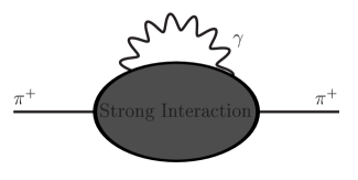
Figure 14: The electromagnetic contribution to the $\pi^{+}$-$\pi^{0}$ mass difference.

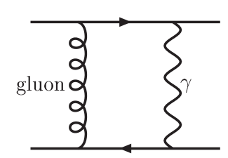
Figure 15: The short-distance photon-gluon box diagram leading to a four-quark operator.

The matrix element involves an integral over all photon momenta

$$M=\displaystyle\int_{0}^{\infty}dq_{\gamma}^{2}\,.$$ (64)

We now split the integral at the arbitrary scale $\mu^{2}$. The short-distance part of the integral, $\displaystyle\int_{\mu^{2}}^{\infty}dq_{\gamma}^{2}$, can be evaluated using OPE techniques $\!{}^{{\bf?}}$ via the box diagram of Fig. 15. Other types of contributions are suppressed by extra factors of $1/\mu^{2}$. The resulting four-quark operator $\displaystyle(\bar{q}q)(\bar{q}q)$ can be estimated in large $N_{c}$$\!{}^{{\bf?}}$

$$\left.m_{\pi^{+}}^{2}-m_{\pi^{0}}^{2}\right|_{\mbox{SD}}=\frac{3\alpha_{S}\alpha_{e}}{\mu^{2}F^{4}}\langle\bar{q}q\rangle^{2}\,.$$ (65)

The long-distance contribution,$\displaystyle\int_{0}^{\mu^{2}}dq_{\gamma}^{2}$, can be evaluated in several ways. CHPT at order $p^{2}$ or $p^{4}$ $\!{}^{{\bf?}}$, a vector meson dominance model(VMD) $\!{}^{{\bf?}}$, the ENJL model $\!{}^{{\bf?}}$ or LMD.$\!{}^{{\bf?}}$

Figure 16: The Short-distance contribution (SD) and the various versions of the long-distance contributions to $m_{\pi^{2}}-m_{\pi^{0}}^{2}$. Also shown are the experimental value and the experimental value minus the chiral logarithms that are extra.

The results are shown in Fig. 16. Notice that the sum of long- and short- distance contributions is quite stable in the regime $\mu\approx 500~{}$MeV to 1 GeV. VMD and LMD are the same in this case.

The main comments to be remembered are:

• The photon couplings are known everywhere.

• We have a good identification of the scale $\mu$. It can be identified from the photon momentum which is unambiguous.

• In the end we got good matching, $\mu$-independence, and the numbers obtained agreed (maybe too) well with the experimental result.

6.6 The $X$-boson method.

The improved factorization model is scheme- and scale-independent but depends on the particular choice of quark/gluon state. Now, photons are identifiable across theory boundaries, or more generally, currents are . An example of this is CHPT where the currents are the same as in QCD.

We can now try to get our four-quark operators back into something resembling a photon so we can use the same method as in the previous section. The full description including all formulas can be found in Ref. [References]. Similar work has been done by Bardeen.$\!{}^{{\bf?}}$ For $\hat{B}_{K}$ this can be done by replacing

$${\cal H}_{\mbox{eff}}^{\Delta S=2}\quad\mbox{ by }\quad g_{X}X_{\Delta S=2}^{\mu}\left(\bar{s}_{\alpha}\gamma_{\mu}d_{\alpha}\right)_{L}\,.$$ (66)

with $M_{X}$ chosen such that $\alpha_{S}\log\frac{M_{X}}{\mu}$ is small and we can neglect higher orders in $\mu^{2}/M_{X}^{2}$.

We now take the matrix element of ${\cal H}_{\mbox{eff}}$ between quark and gluon external states which yields from the diagrams in Fig. 17

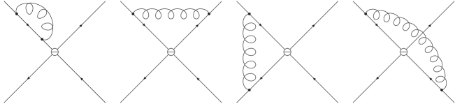
Figure 17: The diagrams for the matrix-element of ${\cal H}_{\mbox{eff}}$ at one-loop.

$$\displaystyle iC_{D}\left[\left(1+\alpha_{S}(\nu)F(q_{i})\right)S_{1}+\left(1+\alpha_{S}(\nu)F^{\prime}(q_{i})\right)S_{2}\right]$$

$$C_{D}=-C(\nu)\left(1+\frac{\alpha_{S}(\nu)}{\pi}\left[\frac{\gamma_{1}}{2}\ln\left(\frac{2q_{1}\cdot q_{2}}{\nu^{2}}\right)+r_{1}\right]\right)$$ (67)

with $S_{1}$ and $S_{2}$ the tree level matrix elements between quarks of $(\bar{s}\gamma^{\mu}d)_{L}(\bar{s}\gamma_{\mu}d)_{L}$.

We then calculate the same matrix element using $X$-boson exchange from the diagrams in Fig. 18

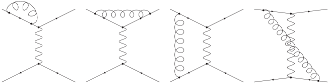
Figure 18: The same matrix element but now of $X$-boson exchange. The wiggly line is the $X$-boson.

and get

$$\displaystyle\hskip-42.67912ptiC_{C}\left[\left(1+\alpha_{S}(\mu_{C})F(q_{i})\right)S_{1}+(1+\alpha_{S}(\mu_{C})F^{\prime}(q_{i}))S_{2}\right]+{\cal O}(M_{X}^{-4})$$

$$C_{C}=\frac{-g_{X}^{2}}{M_{X}^{2}}\left(1+\frac{\alpha_{S}(\mu_{C})}{\pi}\left[\frac{\gamma_{1}}{2}\ln\left(\frac{2q_{1}\cdot q_{2}}{M_{X}^{2}}\right)+\tilde{r}_{1}\right]\right)$$ (68)

Notice that all the dependence on the external quark/gluon state in the functions $F(q_{i})$ and $F^{\prime}(q_{i})$ cancels. $r_{1}$ removes the scheme dependence and $\tilde{r}_{1}$ changes to the $X$-boson current scheme.

$g_{X}$ is now scale, scheme and external quark-gluon state independent. It still depends on the precise scheme used for the vector and axial-vector current.

The $\Delta S=1$ case is more complicated, everything becomes 10 by 10 matrices but can be found in Ref. [References]. The precise definition of the total number of $X$-bosons needed to discuss this case is

$$\displaystyle g_{1}X_{1}^{\mu}\left((\bar{s}\gamma_{\mu}d)_{L}+(\bar{u}\gamma_{\mu}u)_{L}\right)+g_{2}X_{2}^{\mu}\left((\bar{s}\gamma_{\mu}u)_{L}+(\bar{u}\gamma_{\mu}d)_{L}\right)$$

$$\displaystyle+g_{3}X_{3}^{\mu}\left((\bar{s}\gamma_{\mu}d)_{L}+\sum_{q=u,d,s}(\bar{q}\gamma_{\mu}q)_{L}\right)+g_{4}\sum_{q=u,d,s}X_{q,4}^{\mu}\left((\bar{s}\gamma_{\mu}q)_{L}+(\bar{q}\gamma_{\mu}d)_{L}\right)$$

$$\displaystyle+g_{5}X_{5}^{\mu}\left((\bar{s}\gamma_{\mu}d)_{L}+\sum_{q=u,d,s}(\bar{q}\gamma_{\mu}q)_{R}\right)+g_{6}\sum_{q=u,d,s}X_{q,6}\left((\bar{s}q)_{L}+(-2)(\bar{q}d)_{R}\right)$$

$$\displaystyle+g_{7}X_{7}^{\mu}\left((\bar{s}\gamma_{\mu}d)_{L}+\sum_{q=u,d,s}\frac{3}{2}e_{q}(\bar{q}\gamma_{\mu}q)_{R}\right)$$

$$\displaystyle+g_{8}\sum_{q=u,d,s}X_{q,8}\left((\bar{s}q)_{L}+(-2)\frac{3}{2}e_{q}(\bar{q}d)_{R}\right)$$

$$\displaystyle+g_{9}X_{9}^{\mu}\left((\bar{s}\gamma_{\mu}d)_{L}+\sum_{q=u,d,s}\frac{3}{2}e_{q}(\bar{q}\gamma_{\mu}q)_{L}\right)$$

$$\displaystyle+g_{10}\sum_{q=u,d,s}X_{q,10}^{\mu}\left((\bar{s}\gamma_{\mu}q)_{L}+\frac{3}{2}e_{q}(\bar{q}\gamma_{\mu}d)_{L}\right).$$ (69)

The resulting change from this correction is displayed in columns 4 and 5 of Table 3. The corrections are substantial and turn out to be in the wanted direction in all cases, surprisingly enough.

So let us summarize the $X$-boson scheme

1. Introduce a set of fictitious gauge bosons: $X$

2. $\alpha_{S}\log({M_{X}}/{\mu})$ does not need resumming, this is not large.

3. $X$-bosons must be uncolored.

4. Only perturbative QCD and OPE have been used so far.

5. For $\hat{B}_{K}$ we need $r_{1}-\tilde{r}_{1}=-\frac{11}{12}$.

6.7 $X$-boson scheme matrix element: $\hat{B}_{K}$

We now need to calculate $\langle\mbox{out}|X\mbox{-exchange}|\mbox{in}\rangle$. First we do the same split in the $X$-boson momentum integral as we did for the photon

$${\int dq_{X}^{2}}\quad\Longrightarrow\quad{\int_{0}^{\mu^{2}}dq_{X}^{2}+\int_{\mu^{2}}^{\infty}dq_{X}^{2}}$$ (70)

For $q^{2}_{X}$ large, the kaon-form-factor suppresses direct mesonic contributions by $1/q_{X}^{2}$. Large $q_{X}^{2}$ must thus flow back via quarks-gluons. The results are already suppressed by $1/N_{c}$ so we can use leading $1/N_{c}$ in this part. This part ends up replacing $\displaystyle\log\frac{\mu_{OPE}}{M_{X}}$ by $\log\frac{\mu_{OPE}}{\mu}$ such that, as it should be, the dependence on $M_{X}$ has disappeared completely.

For the small $q^{2}_{X}$ integral we now successively use better approximations in 3 directions:

• Low-energy that better approximates perturbative QCD

• Inclusion of quark-masses

• Inclusion of electromagnetism

The last step at present everyone only does at short-distance. One of the problems in the calculations is that Chiral Symmetry provides very strong constraints, which lead to large cancellations between different parts. It is therefore important that all contributions are calculated with a similar scheme to take care of these cancellations correctly.

A few comments are appropriate:

• The Chiral Quark Model approach $\!{}^{{\bf?}}$ does not do the identification of scales and we do not include their results. But they stressed large effects from FSI, quark-masses when factorization+small variations was the main method. See also Ref. [References].

• For some matrix-elements CHPT allows to relate them to integrals over measurable spectral functions. The remainder agrees numerically for these $B_{7},m_{\pi^{+}}^{2}-m_{\pi^{0}}^{2}$. This is discussed in more detail in Sect. 6.9.

The different results for $B_{K}(\mu)$ in the chiral limit are

$$B_{K}^{\chi}(\mu) = \frac{3}{4}\left[1\mbox{ (large-$N_{c}$)}-\frac{3\mu^{2}}{16\pi^{2}F_{0}^{2}}\mbox{ ($p^{2}$)}\right.$$ (71)

$$\left.+\frac{6\mu^{4}}{16\pi^{2}F_{0}^{4}}\left(2L_{1}+5L_{2}+L_{3}+L_{9}\right)\mbox{ ($p^{4}$)}\right]$$

for CHPT $\!{}^{{\bf?},{\bf?}}$. The ENJL model we do numerically $\!{}^{{\bf?},{\bf?}}$ and LMD gives  $\!{}^{{\bf?}}$

$$B_{K}^{\chi}(\mu) = \frac{3}{4}\left\{1-\frac{1}{32\pi^{2}F_{0}^{2}}\right.\int_{0}^{\mu^{2}}dQ^{2}\times$$ (72)

$$\left.\left(6-\sum_{i=res}\left[\frac{\alpha_{i}}{Q^{2}+M_{i}^{2}}-\frac{\alpha_{i}}{M_{i}^{2}}+\frac{\beta_{i}}{(Q^{2}+M_{i}^{2})^{2}}-\frac{\beta_{i}}{M_{i}^{4}}\right]\right)\right\}$$

$\alpha_{i}$ and $\beta_{i}$ are particular combinations of the resonance couplings. These we can now restrict by comparing CHPT and LMD,

$$\sum_{i}\frac{\alpha_{i}}{M_{i}^{4}}+\frac{\beta_{i}}{M_{i}^{6}}=\frac{24}{F_{0}^{2}}\left(2L_{1}+5L_{2}+L_{3}+L_{9}\right)\,,$$ (73)

and using the short-distance constraints:

$$\displaystyle\sum_{i}\left(\alpha_{i}M_{i}^{2}-\beta_{i}\right) = 0$$

$$\sum_{i}\left(\frac{\alpha_{i}}{M_{i}^{2}}+\frac{\beta_{i}}{M_{i}^{4}}\right) = 6$$

$$\sum_{i}\alpha_{i} = 24\pi^{2}\frac{\alpha_{S}}{\pi}F_{0}^{2}\,.$$ (74)

The last requirement is from explicitly requiring matching. The various long distance contributions in the chiral limit and in the presence of masses are shown in Fig. 19.

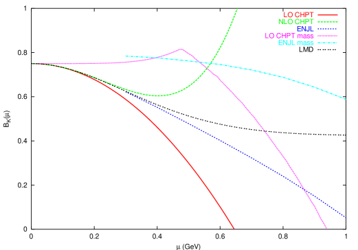
Figure 19: Comparison of the long-distance contributions to $B_{K}$ in the various approximations discussed in the text.

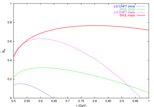
Figure 20: Using the long-distance depicted in Fig. 19 we obtain as results for $\hat{B}_{K}$ as a function of $\mu$.

Including the short-distance part leads to the results for $\hat{B}_{K}$ shown in Fig. 20 and

$$\hat{B}_{K}^{\chi} = 0.32\pm 0.06~{}(\alpha_{S})\pm 0.12~{}(\mbox{model})$$

$$\hat{B}_{K} = 0.77\pm 0.05~{}(\alpha_{S})\pm 0.05~{}(\mbox{model})\,.$$ (75)

The LMD model leads to somewhat higher but compatible results for the chiral case.$\!{}^{{\bf?}}$ The results just using CHPT are also very similar but have worse matching.$\!{}^{{\bf?}}$ The original results of Ref. [References] have been corrected for a correct momentum identification in Ref. [References] and Ref. [References].

6.8 $X$-boson method results for $\Delta I=1/2$ rule and $\varepsilon^{\prime}/\varepsilon$.

We now present the results of the $X$-boson method also for the $\Delta S=1$ quantities. For other approaches I refer to the original references and various talks.$\!{}^{{\bf?}}$

The notation used below and more extensive discussions can be found in Ref. [References].

The lowest-order CHPT Lagrangian for the non-leptonic $\Delta S=1$ sector is given by

$${\cal L}_{\Delta S=1} = -CF_{0}^{4}\,\left[{G_{8}}\,\mbox{tr}(\Delta_{32}u_{\mu}u^{\mu})+\,{G_{8}^{\prime}}\,\mbox{tr}(\Delta_{32}\chi_{+})\right.$$ (76)

$$+{G_{27}}\,t^{ijkl}\mbox{tr}(\Delta_{ij}u_{\mu}u^{\mu})\mbox{tr}(\Delta_{kl}u_{\mu}u^{\mu})\left.+{e^{2}G_{E}}F_{0}^{2}\mbox{tr}(\Delta_{32}\tilde{Q})\right];$$

and contains four couplings, The various notations used are

$$U\equiv\exp\left({i\sqrt{2}\Phi/F_{0}}\right)\equiv u^{2}\,; u_{\mu}\equiv iu^{\dagger}(D_{\mu}U)u\,;$$

$$\chi_{+}\equiv 2B_{0}\left(u^{\dagger}{\cal M}u^{\dagger}+u{\cal M}^{\dagger}u\right)\, \Delta_{ij}=u\lambda_{ij}u^{\dagger}\,;$$

$$(\lambda_{ij})_{ab}=\delta_{ia}\delta_{jb}\,; \tilde{Q}=u^{\dagger}Qu\,;$$

$$C=\frac{3G_{F}}{5\sqrt{2}}V_{ud}V_{us}^{*}\,.$$ (77)

This notation is very similar to the notation used by Leutwyler for CHPT in his chapter.

Fixing the parameters from $K\to\pi\pi$ allows to predict $K\to 3\pi$ to about 30%. This we discuss in Sect. 7.

In the limit $N_{c}\to\infty$ & $e\to 0$ the parameters become

$$G_{8},\,G_{27}\longrightarrow 1\,;\quad G_{8}^{\prime},\,e^{2}G_{E}\longrightarrow 0\,.$$ (78)

The normalization of $G_{8}$ and $G_{27}$ was chosen in order to have this simple limit.

The isospin 0 and 2 amplitudes for $K\to\pi\pi$ from the above Lagrangian are

$${a_{0}} = \frac{\sqrt{6}}{9}\,CF_{0}\left[\left(9G_{8}+G_{27}\right)(m_{K}^{2}-m_{\pi}^{2})-6e^{2}G_{E}F_{0}^{2}\right]$$

$${a_{2}} = \frac{\sqrt{3}}{9}\,CF_{0}\left[10G_{27}\,(m_{K}^{2}-m_{\pi}^{2})-6e^{2}G_{E}F_{0}^{2}\right]\,.$$ (79)

The experimental values are $\!{}^{{\bf?},{\bf?}}$ Re$(G_{8})\approx 6.2$ and Re$(G_{27})\approx 0.48$ with a sizable error.

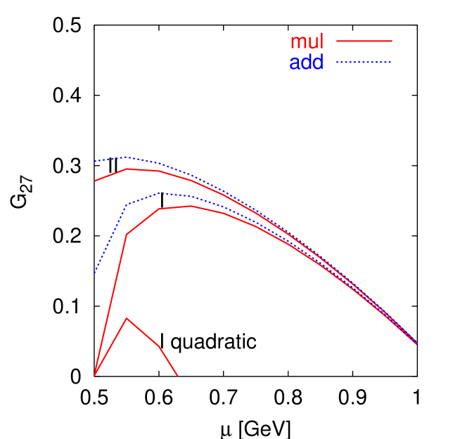
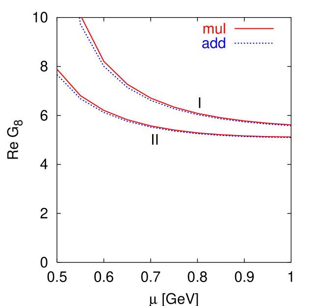
Figure 21: Results for the real part of the $\Delta S=1$ chiral Lagrangian. Remember that $\mbox{Re}G_{8}^{\mbox{exp}}\approx 6.2$ and $\mbox{Re}G_{27}^{\mbox{exp}}\approx 0.48$. The labels I and II refer to two different values of $\alpha_{S}$ and mul-add to two ways of combining the various QCD corrections, differing only at higher orders.

The results obtained are shown in Fig. 21 for the real parts and in Fig. 22 for the imaginary parts. Notice that we get good matching for most quantities and good agreement with the experimental result for $G_{8}$. The bad matching for $G_{27}$ is because we have a large cancellation needed between the non-factorizable and the factorizable case to obtain matching. The 30% or so accuracy we have on the non-factorizable part leads therefore to large errors on the final result. Notice that all methods that do not impose the matching by hand, typically have a problem with this. The other quantities are not affected by such a cancellation and show therefore better matching.

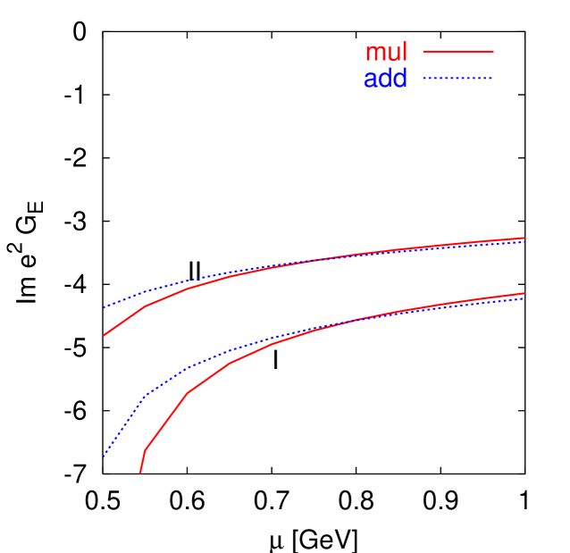
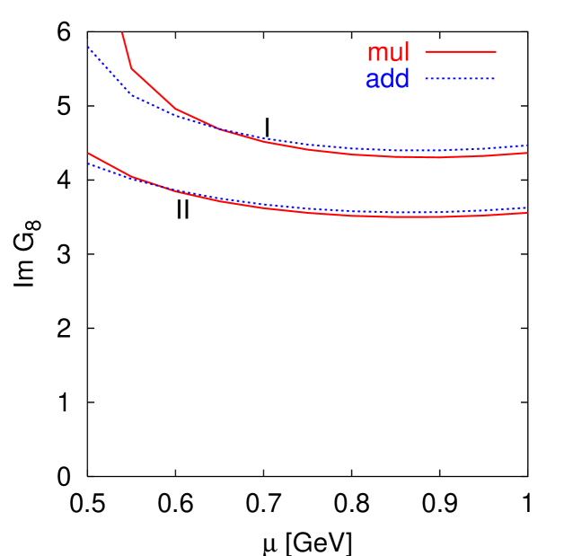
Figure 22: Results for the imaginary part of the $\Delta S=1$ chiral Lagrangian.

The origin of the large enhancement for $G_{8}$ is in the long-distance Penguin diagrams. The long distance calculations contains contributions that have the same quark line structure of the gluonic Penguin diagram. It is these that provide the extra enhancement. Otherwise we would have the relation to next-to-leading order in $1/N_{c}$ of $1-G_{27}=G_{8}-1$.$\!{}^{{\bf?}}$

We can now use the above results to estimate $\varepsilon^{\prime}/\varepsilon$ in the chiral limit. We used $G_{27}=0.48$, $\mbox{Re}G_{8}=6.2$ and the values we obtained for the imaginary part. The same method leads to $\varepsilon$ within 10% of the experimental value. The result is shown in Fig. 23.

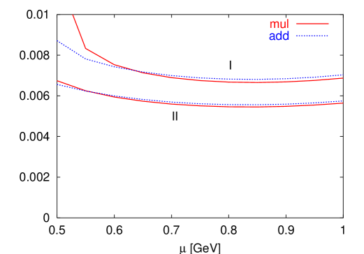
Figure 23: The results for $\varepsilon^{\prime}/\varepsilon$ in the chiral limit. Notice the quite good matching.

We can conclude that

$$\left(\frac{\varepsilon^{\prime}}{\varepsilon}\right)^{\chi}=(7.4-1.9)\cdot 10^{-3}=5.5\cdot 10^{-3}$$ (80)

and
$\bullet$ $B_{6}\approx 2.5$ not $\lesssim 1.5$
$\bullet$ $B_{8}\approx 1.3$ OK but not $B_{8}\approx B_{6}$ .

Using

$$|\varepsilon^{\prime}|\simeq\frac{1}{\sqrt{2}}\frac{\mbox{Re}\,a_{2}}{\mbox{Re}\,a_{0}}\left(-\frac{\mbox{Im}\,a_{0}}{\mbox{Re}\,a_{0}}+\frac{\mbox{Im}\,a_{2}}{\mbox{Re}\,a_{2}}\right)$$ (81)

We can now include the two main known corrections. The usual approach for final state interactions (FSI) is to take $\mbox{Re}a_{0}$, $\mbox{Re}a_{2}$ from experiment and $\mbox{Im}a_{0}$, $\mbox{Im}a_{2}$ to ${\cal O}(p^{2})$. This leads to a large suppression of the first term in Eq. (81).$\!{}^{{\bf?}}$ We evaluate both to $p^{2}$ so for us FSI act mainly on the prefactor in Eq. (81).

The main isospin breaking correction is that $\pi^{0}$,$\eta$ and $\eta^{\prime}$ mix. This, together with the other isospin breaking corrections, brings in a part of the large $a_{0}$ into $a_{2}$ and is thus enhanced. The effect is usually parametrized as

$$\frac{\Delta\mbox{Im}a_{2}}{\mbox{Re}a_{2}}\approx\Omega\frac{\mbox{Im}a_{0}}{\mbox{Re}a_{0}}\quad\mbox{with}\quad\Omega\approx 0.16\pm 0.03$$ (82)

where the numerical value is taken from Ref. [References]. There is, in addition to Ref. [References] a rather large body of recent work on electromagnetic and isospin corrections.$\!{}^{{\bf?}}$

Including the last two main corrections yields

$$\left|\frac{\varepsilon^{\prime}}{\varepsilon}\right|=(5.4-2.3)\cdot 10^{-3}=(3.1\pm??)\cdot 10^{-3}\,.$$ (83)

The size of the error is debatable but should be at least 50% given all the uncertainties involved.

6.9 Dispersive Work and Higher Order Operators

Some of the matrix elements we want here can be extracted from experimental information in a different way. The canonical example is the mass difference between the charged and the neutral pion in the chiral limit which can be extracted from a dispersive integral over the difference of the vector and axial vector spectral functions.$\!{}^{{\bf?}}$

This idea has been pursued in the context of weak decay in a series of papers by Donoghue, Golowich and collaborators.$\!{}^{{\bf?}}$ The matrix element of $Q_{7}$ could be extracted directly from these data. To get at the matrix element of $Q_{8}$ is somewhat more difficult. Ref. [References] extracted it first by requiring $\mu$-independence. In the first paper cited in Ref. [References], it was realized that the matrix element of $Q_{8}$ could also be extracted from the spectral functions and was related to the coefficient of the dimension 6 term in the operator product expansion of the underlying Green’s function. The most recent papers using this method are Refs. [References], [References], [References] and [References]. In the last two papers also some QCD corrections were included which had a substantial impact on the numerical results.

The results are given in Table. 4. The operator $O_{6}^{(1)}$ is related by a chiral transformation to $Q_{7}$ and $O_{6}^{(2)}$ to $Q_{8}$. The numbers are valid in the chiral limit.

Reference	$\langle 0|O_{6}^{(1)}|0\rangle^{NDR}_{\chi}$	$\langle 0|O_{6}^{(2)}|0\rangle^{NDR}_{\chi}$
$B_{7}=B_{8}=1$	$-(5.4\pm 2.2)\cdot 10^{-5}$ GeV6	$(1.0\pm 0.4)\cdot 10^{-3}$ GeV6
Bijnens et al. $\!{}^{{\bf?}}$	$-(4.0\pm 0.5)\cdot 10^{-5}$ GeV6	$(1.2\pm 0.5)\cdot 10^{-3}$ GeV6
Knecht et al. $\!{}^{{\bf?}}$	$-(1.9\pm 0.6)\cdot 10^{-5}$ GeV6	$(3.5\pm 1.1)\cdot 10^{-3}$ GeV6
Cirigliano et al. $\!{}^{{\bf?}}$	$-(2.7\pm 1.7)\cdot 10^{-5}$ GeV6	$(2.2\pm 0.7)\cdot 10^{-3}$ GeV6
Donoghue et al.$\!{}^{{\bf?}}$	$-(4.3\pm 0.9)\cdot 10^{-5}$ GeV6	$(1.5\pm 0.4)\cdot 10^{-3}$ GeV6
Narison $\!{}^{{\bf?}}$	$-(3.5\pm 1.0)\cdot 10^{-5}$ GeV6	$(1.5\pm 0.3)\cdot 10^{-3}$ GeV6
lattice $\!{}^{{\bf?}}$	$-(2.6\pm 0.7)\cdot 10^{-5}$ GeV6	$(0.74\pm 0.15)\cdot 10^{-3}$ GeV6
ENJL $\!{}^{{\bf?}}$	$-(4.3\pm 0.5)\cdot 10^{-5}$ GeV6	$(1.3\pm 0.2)\cdot 10^{-3}$ GeV6

Table 4: The values of the VEVs in the NDR scheme at $\mu_{R}=2$ GeV. The most recent dispersive results are line 3 to 5. Adapted from Ref. [References].

The various results for the matrix element of $O_{6}^{(1)}$ are in reasonable agreement with each other. The underlying spectral integral, evaluated directly from data in Refs. [References],[References] and [References], or via the minimal hadronic ansatz $\!{}^{{\bf?}}$ are in better agreement. The main difference is that the number quoted for Ref. [References] does not include the extra QCD corrections. The largest source of the differences is the way the different results for the underlying evaluation of $O_{6}^{(2)}$ come back into $O_{6}^{(1)}$.

The results for $O_{6}^{(2)}$ differ more. Ref. [References] uses two approaches. First, the matrix element for $O_{6}^{(2)}$ can be extracted via a similar dispersive integral over the scalar and pseudoscalar spectral functions. The requirements of short-distance matching for this spectral function combined with a saturation with a few states imposes that the nonfactorizable part is suppressed and the number and error quoted follows from this. Extracting the coefficient of the dimension 6 operator in the expansion of the vector and axial-vector spectral functions yields a result comparable but with a larger error of about 0.9. Ref. [References] chose to enforce all the known constraints on the vector and axial-vector spectral functions to obtain a result. This resulted in rather large cancellations between the various contributions making an error analysis more difficult. A reasonable estimate lead to the value quoted. Ref. [References] did not include the extra QCD correction which lowers the value. The number quoted is derived by a single resonance plus continuum ansatz for the spectral functions and assuming a typical large $N_{c}$ error of 30%. This ansatz worked well for lower moments of the spectral functions which can be tested experimentally. Adding more resonances allows for a broader range of results.$\!{}^{{\bf?}}$ The reason why these numbers based on the same data can be so different is that the quantity in question is sensitive to the energy regime above 1.3 GeV where the accuracy of the data is rather low.

7 CHPT tests in non-leptonic Kaon decays to pions

The use of current algebra methods in kaon decays to pions goes back a long time.$\!{}^{{\bf?}}$ In Ref. [References] the full lowest order CHPT contributions were worked out for kaon decays to pions using current algebra methods. Later it was realized $\!{}^{{\bf?}}$ that $B_{K}$ could be determined from the $\Delta I=3/2$ part of $K\to\pi\pi$ and a substantial deviation from the vacuum saturation value was found, about $0.3$ instead of $1$. It was found later that this particular 3-flavour chiral symmetry relation has potentially large corrections $\!{}^{{\bf?}}$ and the full analysis of Ref. [References,References] showed that there are free parameters in this relation. Nevertheless, CHPT is still useful for nonleptonic kaon decays for connecting $K\to\pi\pi$ to $K\to\pi\pi\pi$.

I have already shown the lowest order $\Delta S=1$ CHPT Lagrangian in Eq. (76) and mentioned that this reproduces $K\to\pi\pi\pi$ to about 30% from $K\to\pi\pi$. This can be extended to an order $p^{4}$ calculation in CHPT $\!{}^{{\bf?},{\bf?}}$. The chiral logarithms for $K\to\pi\pi$ were known earlier.$\!{}^{{\bf?}}$ The diagrams needed, now the lines are mesons, not quarks as in most of the previous figures, are shown in Fig. 24 for $K\to\pi\pi$. The $K\to\pi\pi\pi$ ones are similar.

Figure 24: The CHPT diagrams with meson loops at order $p^{4}$ for $K\to\pi\pi$.

In terms of the number of parameters and observables we have

# parameters :	$p^{2}$ :	2 (1)	$G_{8}$, $G_{27}$
	$p^{4}$ :	7(3)	($-2$ that cannot be disentangled
			from $G_{8}$, $G_{27}$)
# observables:	After isospin
$K\to 2\pi$ :	2(1)
$K\to 3\pi$ :	2(1)+1		constant in Dalitz plot
	3(1)+3		linear
	5(1)		quadratic

Phases (the +i above) of up to linear terms in the Dalitz plot might also be measurable. The numbers in brackets refer to $\Delta I=1/2$ parameters and observables only. Notice that a significant number of tests is possible. Comparison with the present data is shown in Table 5. The numbers in brackets refer to which inputs produce which predictions.

variable	$p^{2}$	$p^{4}$	experiment
$\alpha_{1}$	74	(1)input	91.71$\pm$0.32
$\beta_{1}$	$-$16.5	(2)input	$-$25.68$\pm$0.27
$\zeta_{1}$		(1)$-$0.47$\pm$0.18	$-$0.47$\pm$0.15
$\xi_{1}$		(2) $-$1.58$\pm$0.19	$-$1.51$\pm$0.30
$\alpha_{3}$	$-$4.1	(3) input	$-$7.36$\pm$0.47
$\beta_{3}$	$-$1.0	(4) input	$-$2.42$\pm$0.41
$\gamma_{3}$	1.8	(5) input	2.26$\pm$0.23
$\xi_{3}$	6	(4) 0.92$\pm$0.030	$-$0.12$\pm$0.17
$\xi_{3}^{\prime}$		(5) $-$0.033$\pm$0.077	$-$0.21$\pm$0.51
$\zeta_{3}$		(3) $-$0.0011$\pm$0.006	$-$0.21$\pm$0.08

Table 5: CHPT to order $p^{4}$ for $K\to\pi\pi\pi$. The variables refer to various measurables in the Dalitz plot. $K\to\pi\pi$ is always used as input. Numbers in brackets indicate relations.

It is important that in the future experiments tests these relations directly. At present there is satisfactory agreement with the data. Notice that the new CPLEAR data decrease the errors somewhat. A recalculation of this process together with a fit to the newer data is in progress.$\!{}^{{\bf?}}$

CP-violation in $K\to 3\pi$ will be very difficult. The strong phases needed to interfere are just too small (Ref. [References] last reference). E.g. $\delta_{2}-\delta_{1}$ in $K_{L}\to\pi^{+}\pi^{-}\pi^{0}$ is expected to be $-0.083$ and the present experimental bound is only $-0.33\pm 0.29$. The CP-asymmetries expected are about $10^{-6}$ so we expect in the near future only to improve limits. A review of $CP$ violation in $K\to 3\pi$ can be found in Ref. [References].

8 Kaon rare decays

The below is a summary of the summary by Isidori given at KAON99 and LP01 and Buchalla in KAON2001.$\!{}^{{\bf?}}$ I refer there for references. Another somewhat older but more extensive review is Ref. [References] and I also found Ref. [References] useful.

Some of the processes mentioned below are tests of strong interaction physics, often in the guise of CHPT, and others are mainly SM tests.

• $\mathbf{K}^{+}\to\pi^{+}\nu\bar{\nu}$,$\mathbf{K}_{L}\to\pi^{0}\nu\bar{\nu}$ In this case the SM is strongly suppressed and dominated by short-distance physics. It is thus ideal for precision SM CKM tests and possibly new physics searches. The reason is that real and imaginary part of the amplitude are similar here in size, CKM angle suppression is counteracted by the large top-quark mass. This allows it to be dominated by $\bar{s}dZ$-Penguin and $WW$-box diagrams. The resulting

  $${\cal H}_{\mbox{eff}}=C_{\nu}(\bar{s}\gamma_{\mu}d)_{L}(\bar{\nu}\gamma^{\mu}\nu)_{L}$$ (84)

  can be hadronized using the measured matrix-element from $K_{\ell 3}$ and the $\bar{\nu}\nu$ pair is in a CP eigenstate allowing lots of CP-tests. The main disadvantage is the extremely low predicted branching ratio of

  Neutral mode: $$(3.1\pm 1.3)\cdot 10^{-11}$$

  Charged mode: $$(8.2\pm 3.2)\cdot 10^{-11}$$ (85)

  This process will be competitive with $B$-decays in next generation of kaon experiments.

• $\mathbf{K}_{L}\to\ell^{+}\ell^{-}$: The short-distance contribution comes from $Z$-penguin and boxes. The main uncertainty comes from the long-distance 2$\gamma$ intermediate state.

  $K_{L}\to\mu^{+}\mu^{-}$ dominated by unitary part of $K_{L}\to\gamma\gamma$, which can be taken from the branching ratio for that decay. It fits the data well.

  The long distance part of $K_{L}\to e^{+}e^{-}$ is more dependent on the contributions with off-shell photons. Here there is still work to do.

• $\mathbf{K}\to\pi\ell^{+}\ell^{-}$ The real parts can be predicted by CHPT at order $p^{4}$ from 2 parameters, it fits well. For the imaginary part there are problems with long-distance contributions from $K\to\pi\gamma\gamma$. but the CP-violating quantities are often dominated by direct part.

• $\mathbf{K}_{S}\to\gamma\gamma$ This process was a parameter-free prediction from CHPT at order $p^{4}$ from the diagrams in Fig. 25.

  

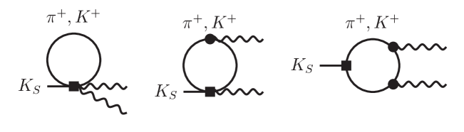
  Figure 25: The meson-loop diagrams contributing to $K_{S}\to\gamma\gamma$. They predict the rate well.

  

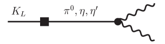
  Figure 26: The main diagram for $K_{L}\to\gamma\gamma$ with a large uncertainty due to cancellations.

• $\mathbf{K}_{L}\to\gamma\gamma$ This decay needs more work. The underlying difficulty is that the main contribution is full of cancellations. The main diagram is shown in Fig. 26.

• $\mathbf{K}_{L}\to\pi^{0}\gamma\gamma$ This process at $p^{4}$ is again a parameter-free CHPT prediction. The spectrum is well described but the rate is somewhat off. This can be explained by $p^{6}$ effects.

• $\mathbf{K}_{S}\to\pi^{0}\gamma\gamma$ This process has very similar problems as $K_{L}\to\gamma\gamma$.

• $\mathbf{K}_{L(S)}\to\gamma^{*}\gamma^{*}$ The same processes as above but with one or both photons off-shell, decaying into a $\ell^{+}\ell^{-}$-pair. These have similar questions/problems/successes as the ones with on-shell photons.

9 Conclusions

In this review I have given a historical overview and an introduction of which sector of the standard model we hope to test using these experiments. The main underlying problem is the strong interaction and I have discussed their impact on the various weak decays of light flavours. The results can be summarized as follows:

• Semi-leptonic Decays

  • CHPT is a major success and tool here.

  • These decays are the main input for $V_{ud}$ and $V_{us}$

  • In addition they provide several tests of strong interaction effects.

• $\mathbf{K}\to\pi\pi$ and $\mathbf{{\overline{K^{0}}}}$-$\mathbf{K}^{0}$ mixing This was the main part of this review. I hope I have convinced you that there is qualitative agreement and successful prediction is in principle possible but more work on including extra effects and pushing down the uncertainty is obviously needed.

• $\mathbf{K}\to\pi\pi\pi$ A good test of CHPT and strong interaction effects but not very promising for CP violation studies.

• Rare Decays. I only presented a very short summary of the issues.

References

- [1]
-
[2]
E. Fermi,
Nuovo Cim. 11, 1 (1934);
E. Fermi, Z. Phys. 88, 161 (1934). - [3] T. D. Lee and C. N. Yang, Phys. Rev. 104, 254 (1956).
- [4] C. S. Wu, E. Ambler, R. W. Hayward, D. D. Hoppes and R. P. Hudson, Phys. Rev. 105, 1413 (1957).
- [5] J. I. Friedman and V. L. Telegdi, Phys. Rev. 105, 1681 (1957).
- [6] E. C. Sudarshan and R. E. Marshak, Phys. Rev. 109, 1860 (1958).
- [7] R. P. Feynman and M. Gell-Mann, Phys. Rev. 109, 193 (1958).
- [8] A. Pais,Phys. Rev. 86, 663 (1952).
- [9] M. Gell-Mann, Phys. Rev. 92, 833 (1953).
- [10] M. Gell-Mann and A. Pais,Phys. Rev. 97, 1387 (1955).
-
[11]
Y. Ne’eman, Nucl. Phys. 26, 222 (1961);
M. Gell-Mann, Phys. Rev. 125, 1067 (1962);
M. Gell-Mann, California Institute of Technology Synchrotron Laboratory Report No. CTSL-20, 1961 (unpublished), - [12] S. Sakata, Progr. Theoret. Phys. (Kyoto) 16, 686 (1956).
- [13] N. Cabibbo, Phys. Rev. Lett. 10, 531 (1963).
-
[14]
M. Gell-Mann,
Phys. Lett. 8, 214 (1964);
G. Zweig, CERN report, unpublished. - [15] J. H. Christenson, J. W. Cronin, V. L. Fitch and R. Turlay, Phys. Rev. Lett. 13, 138 (1964).
- [16] T. T. Wu and C. N. Yang, Phys. Rev. Lett. 13, 380 (1964).
- [17] L. Wolfenstein, Phys. Rev. Lett. 13, 562 (1964).
- [18] T. D. Lee and C. S. Wu, Ann. Rev. Nucl. Part. Sci. 15, 381 (1965).
- [19] T. D. Lee and C. S. Wu, Ann. Rev. Nucl. Part. Sci. 16, 471 (1966).
- [20] T. D. Lee and C. S. Wu, Ann. Rev. Nucl. Part. Sci. 16, 511 (1966).
- [21] C. N. Yang and R. L. Mills, Phys. Rev. 96, 191 (1954).
- [22] S. L. Glashow, Nucl. Phys. 22, 579 (1961).
- [23] S. L. Glashow, J. Iliopoulos and L. Maiani, Phys. Rev. D2, 1285 (1970).
- [24] M. K. Gaillard and B. W. Lee, Phys. Rev. D10, 897 (1974).
- [25] H. Fritzsch, M. Gell-Mann and H. Leutwyler, Phys. Lett. B47, 365 (1973).
-
[26]
D. J. Gross and F. Wilczek,
Phys. Rev. Lett. 30, 1343 (1973);
H. D. Politzer, Phys. Rev. Lett. 30, 1346 (1973). - [27] M. K. Gaillard and B. W. Lee, Phys. Rev. Lett. 33, 108 (1974).
- [28] G. Altarelli and L. Maiani, Phys. Lett. B52, 351 (1974).
- [29] A. I. Vainshtein, V. I. Zakharov, V. A. Novikov and M. A. Shifman, Sov. J. Nucl. Phys. 23, 540 (1976) [Yad. Fiz. 23, 1024 (1976)].
-
[30]
A. I. Vainshtein, V. I. Zakharov and M. A. Shifman,
JETP Lett. 22, 55 (1975)
[Pisma Zh. Eksp. Teor. Fiz. 22, 123 (1975)];
M. A. Shifman, A. I. Vainshtein and V. I. Zakharov, Nucl. Phys. B120, 316 (1977). - [31] M. A. Shifman, A. I. Vainshtein and V. I. Zakharov, Sov. Phys. JETP 45, 670 (1977) [Zh. Eksp. Teor. Fiz. 72, 1275 (1977)].
- [32] A. I. Vainshtein, the 1999 Sakurai Prize Lecture, Int. J. Mod. Phys. A14, 4705 (1999) [hep-ph/9906263].
- [33] M. Kobayashi and T. Maskawa, Prog. Theor. Phys. 49, 652 (1973).
- [34] S. Weinberg, Phys. Rev. Lett. 37, 657 (1976).
- [35] F. J. Gilman and M. B. Wise, Phys. Lett. B83, 83 (1979).
- [36] F. J. Gilman and M. B. Wise, Phys. Rev. D20, 2392 (1979).
- [37] B. Guberina and R. D. Peccei, Nucl. Phys. B163, 289 (1980).
- [38] F. J. Gilman and M. B. Wise, Phys. Lett. B93, 129 (1980).
- [39] F. J. Gilman and M. B. Wise, Phys. Rev. D27, 1128 (1983).
- [40] J. Bijnens and M. B. Wise, Phys. Lett. B137, 245 (1984).
- [41] J. M. Flynn and L. Randall, Phys. Lett. B224, 221 (1989) [Phys. Lett. B235, 412 (1989)].
- [42] G. Altarelli, G. Curci, G. Martinelli and S. Petrarca, Phys. Lett. B99, 141 (1981).
- [43] G. Altarelli, G. Curci, G. Martinelli and S. Petrarca, Nucl. Phys. B187, 461 (1981).
-
[44]
T. van Ritbergen and R. G. Stuart,
Nucl. Phys. B564, 343 (2000)
[hep-ph/9904240];
T. van Ritbergen and R. G. Stuart, Phys. Rev. Lett. 82, 488 (1999) [hep-ph/9808283]. - [45] D. E. Groom et al., Eur. Phys. J. C15, 1 (2000).
- [46] L. Wolfenstein, Phys. Rev. Lett. 51, 1945 (1983).
- [47] C. Jarlskog, Phys. Rev. Lett. 55, 1039 (1985).
- [48] W. S. Woolcock, Mod. Phys. Lett. A6, 2579 (1991).
- [49] A. Garcia, J. L. Garcia-Luna and G. Lopez Castro, Phys. Lett. B500, 66 (2001) [nucl-th/0006037].
- [50] H. Leutwyler, “Chiral dynamics,” Volume 1, [hep-ph/0008124].
- [51] H. Leutwyler and M. Roos, Z. Phys. C25, 91 (1984).
- [52] V. Cirigliano, M. Knecht, H. Neufeld, H. Rupertsberger and P. Talavera, “Radiative corrections to K(l3) decays,” hep-ph/0110153;
- [53] J. Bijnens and P. Talavera, work in progress.
- [54] J. Bijnens, G. Colangelo, G. Ecker and J. Gasser, hep-ph/9411311 in 2nd DAPHNE Physics Handbook.
- [55] J. Bijnens, hep-ph/9907514, talk KAON99.
- [56] A. Afanasev and W. W. Buck, “Form factors of kaon semileptonic decays,” hep-ph/9607445.
- [57] G. Amoros, J. Bijnens and P. Talavera, Nucl. Phys. B568, 319 (2000) [hep-ph/9907264].
- [58] M. Knecht et al.,Eur. Phys. J. C12, 469 (2000) [hep-ph/9909284].
- [59] P. Post and K. Schilcher, “K(l3) form factors at order in chiral perturbation theory,” hep-ph/0112352.
- [60] G. Amoros, J. Bijnens and P. Talavera, Phys. Lett. B480, 71 (2000) [hep-ph/9912398]; Nucl. Phys. B585 (2000) 293 Erratum-ibid. B598, 665 (2001) [hep-ph/0003258].
- [61] J. Bijnens, G. Ecker and J. Gasser, Nucl. Phys. B396, 81 (1993) [hep-ph/9209261].
- [62] L. Ametller et al.,Phys. Lett. B303, 140 (1993) [hep-ph/9302219].
- [63] J. Kambor, J. Missimer and D. Wyler, Phys. Lett. B261, 496 (1991).
- [64] E. de Rafael, “Chiral Lagrangians and kaon CP violation,” TASI lectures, hep-ph/9502254.
- [65] R. Kessler, “Recent KTeV results”, hep-ex/0110020 .
-
[66]
A. Alavi-Harati et al. (KTeV), Phys. Rev. Lett.83, 22 (1999);
V. Fanti et al. (NA48), Phys. Lett. B465, 335 (1999);
H. Burkhart et al. (NA31), Phys. Lett. B206, 169 (1988);
G.D. Barr et al. (NA31), Phys. Lett. B317, 233 (1993);
L.K. Gibbons et al. (E731), Phys. Rev. Lett. 70, 1203 (1993) - [67] L. Iconomidou-Fayard, NA48 Collaboration, “Results on CP Violation from the NA48 Experiment at CERN,” Presented at 20th International Symposium on Lepton and Photon Interactions at High Energies (Lepton Photon 01), Rome, Italy, 23-28 Jul 2001, hep-ex/0110028
- [68] A. J. Buras, “Weak Hamiltonian, CP violation and rare decays,” hep-ph/9806471, Les Houches lectures.
-
[69]
M. K. Gaillard and B. W. Lee,
Phys. Rev. Lett. 33, 108 (1974);
G. Altarelli and L. Maiani, Phys. Lett. B52, 351 (1974);
A. I. Vainshtein, V. I. Zakharov and M. A. Shifman, JETP Lett. 22, 55 (1975);
F. J. Gilman and M. B. Wise, Phys. Rev. D20, 2392 (1979);
B. Guberina and R. D. Peccei, Nucl. Phys. B163, 289 (1980);
J. Bijnens and M. B. Wise, Phys. Lett. B137, 245 (1984);
M. Lusignoli, Nucl. Phys. B325, 33 (1989);
J. M. Flynn and L. Randall, Phys. Lett. B224, 221 (1989). -
[70]
A. J. Buras and P. H. Weisz,
Nucl. Phys. B333, 66 (1990);
A. J. Buras, M. Jamin, E. Lautenbacher and P. H. Weisz, Nucl. Phys. B370, 69 (1992), Addendum-ibid. B375, 501 (1992);
A. J. Buras, M. Jamin and M. E. Lautenbacher, Nucl. Phys. B400, 75 (1993) [hep-ph/9211321];
A. J. Buras, M. Jamin, M. E. Lautenbacher and P. H. Weisz, Nucl. Phys. B400, 37 (1993) [hep-ph/9211304];
M. Ciuchini, E. Franco, G. Martinelli and L. Reina, Nucl. Phys. B415, 403 (1994) [hep-ph/9304257]. - [71] G. Buchalla, A. J. Buras and M. E. Lautenbacher, Rev. Mod. Phys. 68, 1125 (1996) [hep-ph/9512380].
- [72] S. Herrlich and U. Nierste, Nucl. Phys. B476, 27 (1996) [hep-ph/9604330].
- [73] T. Inami and C. S. Lim, Prog. Theor. Phys. 65, 297 (1981) [Erratum-ibid. 65, 1772 (1981)].
- [74] M. A. Shifman, A. I. Vainshtein and V. I. Zakharov, Nucl. Phys. B147, 385 (1979); Nucl. Phys. B147, 448 (1979).
- [75] P. Colangelo and A. Khodjamirian, “QCD sum rules: A modern perspective,” hep-ph/0010175, Volume 3.
- [76] W. A. Bardeen, A. J. Buras and J.-M. Gérard, Phys. Lett. B192, 138 (1987); Nucl. Phys. B293, 787 (1987).
-
[77]
T. Hambye, G. O. Köhler, E.A. Paschos, P.H. Soldan and W.A. Bardeen,
Phys. Rev. D58, 014017 (1998)
[hep-ph/9802300];
T. Hambye, G. O. Köhler and P. H. Soldan, Eur. Phys. J. C10, 271 (1999) [hep-ph/9902334];
T. Hambye, G. O. Köhler, E. A. Paschos and P. H. Soldan, Nucl. Phys. B564, 391 (2000) [hep-ph/9906434]. -
[78]
J. Bijnens, C. Bruno and E. de Rafael,
Nucl. Phys. B390, 501 (1993)
[hep-ph/9206236];
J. Bijnens, Phys. Rept. 265, 369 (1996) [hep-ph/9502335] and references therein. - [79] J. Bijnens and J. Prades, Phys. Lett. B342, 331 (1995) [hep-ph/9409255]; Nucl. Phys. B444, 523 (1995) [hep-ph/9502363].
- [80] J. Bijnens and J. Prades, J. High Energy Phys. 0001, 002 (2000) [hep-ph/9911392].
- [81] J. Bijnens, E. Pallante and J. Prades, Nucl. Phys. B521, 305 (1998) [hep-ph/9801326].
- [82] J. Bijnens and J. Prades, J. High Energy Phys. 9901, 023 (1999) [hep-ph/9811472].
- [83] J. Bijnens and J. Prades, J. High Energy Phys. 0006, 035 (2000) [hep-ph/0005189].
-
[84]
M. Knecht, S. Peris and E. de Rafael,
Phys. Lett. B457, 227 (1999)
[hep-ph/9812471];
S. Peris and E. de Rafael, Phys. Lett. B490, 213 (2000) [hep-ph/0006146]. - [85] A. Pich and E. de Rafael, Nucl. Phys. B358, 311 (1991).
-
[86]
Ref. [References] and
V. Antonelli, S. Bertolini, J. O. Eeg, M. Fabbrichesi and E. I. Lashin, Nucl. Phys. B469, 143 (1996) [hep-ph/9511255];
V. Antonelli, S. Bertolini, M. Fabbrichesi and E. I. Lashin, Nucl. Phys. B469, 181 (1996) [hep-ph/9511341];
S. Bertolini, J. O. Eeg and M. Fabbrichesi, Nucl. Phys. B476, 225 (1996) [hep-ph/9512356];
S. Bertolini, J. O. Eeg, M. Fabbrichesi and E. I. Lashin, Nucl. Phys. B514, 93 (1998) [hep-ph/9706260];
S. Bertolini, J. O. Eeg and M. Fabbrichesi, Phys. Rev. D63, 056009 (2001) [hep-ph/0002234]. - [87] M. Franz, H. C. Kim and K. Goeke, Nucl. Phys. B562, 213 (1999) [hep-ph/9903275].
-
[88]
C. T. Sachrajda,
“Phenomenology from lattice QCD,”
Presented at 20th International Symposium on Lepton and Photon
Interactions at High Energies (Lepton Photon 01), Rome, Italy, 23-28 Jul 2001,
hep-ph/0110304;
G. Martinelli, “Kaon physics from lattice QCD,” hep-ph/0110023. - [89] L. Lellouch and M. Luscher, Commun. Math. Phys. 219, 31 (2001) [hep-lat/0003023].
- [90] L. Maiani and M. Testa, Phys. Lett. B245, 585 (1990).
- [91] K. G. Chetyrkin, A. L. Kataev, A. B. Krasulin and A. A. Pivovarov, Phys. Lett. B174, 104 (1986) [hep-ph/0103230].
-
[92]
L. J. Reinders and S. Yazaki,
Nucl. Phys. B288, 789 (1987);
N. Bilic, C. A. Dominguez and B. Guberina, Z. Phys. C39, 351 (1988);
N. A. Papadopoulos and H. Vogel, Z. Phys. C51, 73 (1991). -
[93]
J. Prades, C. A. Dominguez, J. A. Penarrocha, A. Pich and E. de Rafael,
Z. Phys. C51, 287 (1991);
A. Pich and E. de Rafael, Phys. Lett. B189, 369 (1987);
A. Pich, B. Guberina and E. de Rafael, Nucl. Phys. B277, 197 (1986);
B. Guberina, A. Pich and E. de Rafael, Phys. Lett. B163, 198 (1985);
A. Pich and E. De Rafael, Phys. Lett. B158, 477 (1985). - [94] Hai-Yang Cheng, talk at ICHEP 2000, Osaka, Japan, 27 Jul - 2 Aug 2000, hep-ph/0008284 and references therein.
-
[95]
W. A. Bardeen, J. Bijnens and J. M. Gerard,
Phys. Rev. Lett. 62, 1343 (1989);
J. Bijnens, Phys. Lett. B306, 343 (1993) [hep-ph/9302217]. - [96] J. Bijnens and J. Prades, Nucl. Phys. B490, 239 (1997) [hep-ph/9610360]
- [97] W. A. Bardeen, hep-ph/0112229.
- [98] E. Pallante and A. Pich, Phys. Rev. Lett. 84, 2568 (2000) [hep-ph/9911233]; Nucl. Phys. B592, 294 (2001) [hep-ph/0007208].
- [99] J. Bijnens, J. M. Gerard and G. Klein, Phys. Lett. B257, 191 (1991).
-
[100]
T. Hambye and P. H. Soldan,
Nucl. Phys. Proc. Suppl. 96, 323 (2001)
[hep-ph/0009073];
S. Bertolini, in Proc. of the 5th International Symposium on Radiative Corrections (RADCOR 2000) ed. Howard E. Haber, hep-ph/0101212;
M. Knecht, S. Peris and E. de Rafael, Nucl. Phys. Proc. Suppl. 86, 279 (2000) [hep-ph/9910396]. - [101] A. Pich and E. de Rafael, Phys. Lett. B374, 186 (1996) [hep-ph/9511465].
- [102] G. Ecker, G. Muller, H. Neufeld and A. Pich, Phys. Lett. B477, 88 (2000) [hep-ph/9912264].
-
[103]
V. Cirigliano, J. F. Donoghue and E. Golowich,
Eur. Phys. J. C18, 83 (2000)
[hep-ph/0008290];
Phys. Rev. D61, 093002 (2000)
[hep-ph/9909473];
Phys. Rev. D61, 093001 (2000)
[Erratum-ibid. D63, 059903 (2000)]
[hep-ph/9907341];
C. E. Wolfe and K. Maltman, expansion,” Phys. Rev. D63, 014008 (2001) [hep-ph/0007319];
Phys. Lett. B482, 77 (2000) [hep-ph/9912254];
G. Ecker, G. Isidori, G. Muller, H. Neufeld and A. Pich, Nucl. Phys. B591, 419 (2000) [hep-ph/0006172];
S. Gardner, U. G. Meissner and G. Valencia, Phys. Lett. B508, 44 (2001) [hep-ph/0103144];
S. Gardner and G. Valencia, Phys. Lett. B466, 355 (1999) [hep-ph/9909202]. - [104] T. Das, G. S. Guralnik, V. S. Mathur, F. E. Low and J. E. Young, Phys. Rev. Lett. 18, 759 (1967).
-
[105]
J. F. Donoghue and E. Golowich,
Phys. Lett. B315, 406 (1993)
[hep-ph/9307263];
Phys. Lett. B478, 172 (2000)
[hep-ph/9911309];
V. Cirigliano and E. Golowich, Phys. Lett. B475, 351 (2000) [hep-ph/9912513];
V. Cirigliano, J. F. Donoghue and E. Golowich, J. High Energy Phys. 0010, 048 (2000) [hep-ph/0007196];
V. Cirigliano and E. Golowich, Phys. Rev. D65, 054014 (2002) [hep-ph/0109265]. - [106] M. Knecht, S. Peris and E. de Rafael, Phys. Lett. B508, 117 (2001) [hep-ph/0102017].
- [107] S. Narison, Nucl. Phys. B593, 3 (2001) [hep-ph/0004247]; Nucl. Phys. Proc. Suppl. 96, 364 (2001) [hep-ph/0012019].
- [108] V. Cirigliano, J. F. Donoghue, E. Golowich and K. Maltman, Phys. Lett. B522, 245 (2001) [hep-ph/0109113].
- [109] J. Bijnens, E. Gamiz and J. Prades, J. High Energy Phys. 0110, 009 (2001) [hep-ph/0108240].
- [110] A. Donini, V. Giménez, L. Giusti, and G. Martinelli, Phys. Lett. B470, 233 (1999)
- [111] J. A. Cronin, Phys. Rev. 161, 1483 (1967).
- [112] J. F. Donoghue, E. Golowich and B. R. Holstein, Phys. Lett. B119, 412 (1982).
- [113] J. Bijnens, H. Sonoda and M. B. Wise, Phys. Rev. Lett. 53, 2367 (1984).
-
[114]
J. Kambor, J. F. Donoghue, B. R. Holstein, J. Missimer and D. Wyler,
Phys. Rev. Lett. 68, 1818 (1992);
G. D’Ambrosio, G. Isidori, A. Pugliese and N. Paver, Phys. Rev. D50, 5767 (1994) [hep-ph/9403235]. - [115] J. Bijnens, Phys. Lett. B152, 226 (1985).
- [116] J. Bijnens, P. Dhonte and F. Persson, work in progress.
- [117] G. D’Ambrosio and G. Isidori, Int. J. Mod. Phys. A13, 1 (1998) [hep-ph/9611284].
-
[118]
G. Isidori,
“Standard model vs new physics in rare kaon decays,”
hep-ph/9908399, talk KAON99;
G. Isidori, “Rare decays: Theory vs. experiments,” hep-ph/0110255;
G. Buchalla, “Rare kaon decays: Overview,” hep-ph/0110313. - [119] L. Littenberg and G. Valencia, Ann. Rev. Nucl. Part. Sci. 43, 729 (1993) [hep-ph/9303225].
- [120] A. J. Buras, “CP violation and rare decays of K and B mesons,” hep-ph/9905437, Lake Louise lectures.