SLAC-PUB-8782 April 2002

Supersymmetric Extra Dimensions: Gravitino Effects in Selectron Pair Production

JoAnne L. Hewett and Darius Sadri

Stanford Linear Accelerator Center

Stanford CA 94309, USA

We examine the phenomenological consequences of a supersymmetric bulk in the scenario of large extra dimensions. We assume supersymmetry is realized in the bulk and study the interactions of the resulting bulk gravitino Kaluza-Klein (KK) tower of states, with supersymmetry breaking on the brane inducing a light mass for the zero-mode gravitino. We derive the 4-d effective theory, including the couplings of the bulk gravitino KK states to fermions and their scalar superpartners. The virtual exchange of the gravitino KK states in selectron pair production in polarized $e^{+}e^{-}$ collisions is then examined. We find that the leading order operator for this exchange is dimension six, in contrast to that of bulk graviton KK exchange which induces a dimension eight operator at lowest order. The resulting kinematic distributions for selectron production are dramatically altered from those in $D=4$ supersymmetric scenarios, and can lead to a enormous sensitivity to the fundamental higher dimensional Planck scale, of order $20-25\times\sqrt{s}$.

1 Introduction

There has been much interest recently in the framework, proposed by Arkani-Hamed, Dimopoulos, and Dvali (ADD) [1, 2], which resolves the hierarchy problem by exploiting the geometry of spacetime. In this scenario, the fundamental scale of gravity in a higher $D=4+\delta$ dimensional spacetime is assumed to be of order the electroweak scale $\sim 1$ TeV. The apparent weakness of gravity in our 4-dimensional world originates from the large volume of the additional $\delta$ spatial dimensions. The 4-dimensional Planck scale is no longer a fundamental scale, leaving the electroweak scale as the ultraviolet cut-off of the low-energy effective theory. The gauge hierarchy is thus effectively eliminated and reduced to the more tractable problem of stabilizing the higher dimensional radii [3]. In this scenario, gravity propagates throughout the higher dimensional volume, known as the bulk, whereas the Standard Model (SM) fields are confined to a $3$-dimensional brane, or wall.

In this theory Gauss’ Law relates the Planck scale of the 4-dimensional theory, $M_{P}$, to the fundamental scale of gravity, $M_{D}$, through the volume of the compactified dimensions $V_{\delta}$ via

$$M_{P}^{2}=V_{\delta}M_{D}^{2+\delta}\,,$$ (1)

where $M_{P}=1.2\times 10^{19}$ GeV is the 4-d Planck scale. Setting $M_{D}\sim 1$ TeV then determines the compactification radius $R_{c}$ of the extra dimensions, with the exact relationship being set by the geometry of the compact dimensions. Assuming that the extra dimensions are of toroidal form and are all of equal size, we have $V_{\delta}=(2\pi R_{c})^{\delta}$. $R_{c}$ then ranges from a sub-millimeter to a few fermi for $\delta=2$ to 6. The case of $\delta=1$ is excluded as it predicts corrections to Newtonian gravity at distances comparable to those in the solar system. A similar scenario can be realized in string theory where the string scale plays the role of the higher dimensional fundamental scale [4], with the string scale acting as the ultraviolet cut-off of the theory.

Proposals for the localization of SM matter and gauge fields to a $3+1$ dimensional wall have been made in the context of topological defects of higher dimensional field theories [5]. Such localization can occur naturally in string theory via D-branes where the SM particles are represented by open strings whose ends lie on the D-brane, while gravitons, which carry no gauge charges, may propagate in the bulk and correspond to closed strings [2, 6, 7].

Since this scenario modifies gravity at the electroweak scale, it is natural to expect the emergence of new phenomena at the TeV scale which may reveal itself in experiments and lead to signatures very different from SM predictions. Upon compactification, the bulk graviton expands into a Kaluza-Klein (KK) tower of states, referred to as a bulk graviton KK tower, which interact with the SM fields on the brane. Collider signals for the graviton KK states have been studied by various authors [8, 9], who have considered the virtual exchange of bulk graviton Kaluza-Klein towers, processes which radiate gravitons into the bulk, and stringy excitations of the Standard Model particles. Data from the Tevatron, LEPII, and HERA [10] presently constrain $M_{D}\mathrel{\mathchoice{\lower 3.01385pt\vbox{\halign{$\matth\displaystyle\hfil#\hfil$\cr>\crcr\sim\crcr}}}{\lower 3.01385pt\vbox{\halign{$\matth\textstyle\hfil#\hfil$\cr>\crcr\sim\crcr}}}{\lower 3.01385pt\vbox{\halign{$\matth\scriptstyle\hfil#\hfil$\cr>\crcr\sim\crcr}}}{\lower 3.01385pt\vbox{\halign{$\matth\scriptscriptstyle\hfil#\hfil$\cr>\crcr\sim\crcr}}}}1$ TeV for all values of $\delta$, while the LHC and a future high energy $e^{+}e^{-}$ Linear Collider are expected to probe fundamental scales in the $5-9$ TeV range. Astrophysical and cosmological considerations [11] place stringent bounds, of order $M_{D}\mathrel{\mathchoice{\lower 3.01385pt\vbox{\halign{$\matth\displaystyle\hfil#\hfil$\cr>\crcr\sim\crcr}}}{\lower 3.01385pt\vbox{\halign{$\matth\textstyle\hfil#\hfil$\cr>\crcr\sim\crcr}}}{\lower 3.01385pt\vbox{\halign{$\matth\scriptstyle\hfil#\hfil$\cr>\crcr\sim\crcr}}}{\lower 3.01385pt\vbox{\halign{$\matth\scriptscriptstyle\hfil#\hfil$\cr>\crcr\sim\crcr}}}}100$ TeV, for the case of $\delta=2$; these limits weaken substantially to $M_{D}\mathrel{\mathchoice{\lower 3.01385pt\vbox{\halign{$\matth\displaystyle\hfil#\hfil$\cr>\crcr\sim\crcr}}}{\lower 3.01385pt\vbox{\halign{$\matth\textstyle\hfil#\hfil$\cr>\crcr\sim\crcr}}}{\lower 3.01385pt\vbox{\halign{$\matth\scriptstyle\hfil#\hfil$\cr>\crcr\sim\crcr}}}{\lower 3.01385pt\vbox{\halign{$\matth\scriptscriptstyle\hfil#\hfil$\cr>\crcr\sim\crcr}}}}1$ TeV for higher values of $\delta$. Mechanical experiments have tested the inverse-square nature of the gravitational force law down to distances of $150\mu m$ [12] for the case of $\delta=2$. This scenario is thus consistent with all data as long as the number of extra dimensions is greater than one, with the case of $\delta=2$ being disfavored in terms of being relevant to the hierarchy problem.

While the original motivation for the ADD scenario was to solve the hierarchy problem without the introduction of low-energy supersymmetry (or technicolor), one still might ask whether supersymmetry plays a role in such a scenario. Clearly, bulk supersymmetry is not in conflict with the basic assumptions of the model. In fact, various reasons exist for believing in a supersymmetric bulk, not least of which is the motivation of string theory. As discussed above, D-branes of string theory provide a natural mechanism for the confinement of the SM fields. If string theory is the ultimate theory of nature then the proposal of ADD might be embedded within it with a supersymmetric bulk, i.e., a bulk supporting a supersymmetric gravitational action. In addition, extra dimensional geometries have been shown to provide novel methods for breaking supersymmetry [13, 14], the possibility that a supersymmetric bulk might provide a source for a tiny cosmological constant has been discussed [15], and supersymmetry might also serve as a mechanism for stabilizing the bulk radii. Supersymmetry has also been considered in the context of warped extra dimensions present in the Randall-Sundrum scenario of localized gravity [16].

In this paper, we investigate the consequences of a supersymmetric bulk in the ADD scenario. If bulk supersymmetry remains unbroken away from the brane, then it is natural to ask what happens to the superpartners of the bulk gravitons, the gravitinos. The bulk gravitinos must also expand into a Kaluza-Klein tower of states and induce experimental signatures. Up to now, the phenomenology of such gravitino KK states has been unexplored. The existence of a light graviphoton, which is present if there is no orbifolding, in supersymmetric ADD has been shown to alter the non-supersymmetric ADD phenomenology [17], and hence we also expect large effects from the gravitino sector. Here, for concreteness, we examine the virtual exchange of the bulk gravitino KK tower in superparticle pair production.

We now outline the approach taken in this paper. We study the compactification of the gravitino sector of a generic supergravity theory living in the bulk and work out the form of the effective action describing the free part of the reduced action on the $3+1$ dimensional brane to which the fields of the Minimal Supersymmetric Standard Model (MSSM) are assumed to be confined. We assume that supersymmetry on the wall is broken, giving rise to masses for the zero-modes of the Kaluza-Klein tower resulting from the reduction of the higher dimensional gravitinos, and shifting the masses of all higher modes. We make no special assumptions about the nature or origin of confinement of the MSSM fields to the wall. We then derive the couplings of the Kaluza-Klein modes of the higher dimensional gravitinos to fermions and their scalar superpartners on the wall, yielding an effective 4-d theory which we then use to study the corrections to collider signatures of certain processes in the MSSM. For purposes of illustration, we work with a $10$ dimensional theory; the generality of our results should be apparent (up to considerations of representations of fermions in various dimensions).

The gravitino zero-mode acquires a mass from the spontaneous breaking of supersymmetry on the brane, with this mass being proportional to $\sim\Lambda^{2}_{SUSY}/M_{P}$, where $\Lambda_{SUSY}$ represents the supersymmetry breaking scale in a generic model, noting that the zero-mode gravitino couples with the usual $M_{P}^{-1}$ strength. This familiar 4-d expression can also be seen to arise from the volume factor after integrating over the $\delta$ extra dimensions and using Eq. (1). Various SUSY breaking scenarios thus yield different predictions ranging from ultralight gravitinos from weak-scale supersymmetry breaking models, light gravitinos in gauge mediated SUSY breaking, and heavier gravitinos in models of gravity and anomaly mediated SUSY breaking. The possibility of light gravitinos is an interesting one and their generic collider [18] and astrophysical [19] implications have been studied, with direct collider searches yielding a bound of $m_{3/2}\mathrel{\mathchoice{\lower 3.01385pt\vbox{\halign{$\matth\displaystyle\hfil#\hfil$\cr>\crcr\sim\crcr}}}{\lower 3.01385pt\vbox{\halign{$\matth\textstyle\hfil#\hfil$\cr>\crcr\sim\crcr}}}{\lower 3.01385pt\vbox{\halign{$\matth\scriptstyle\hfil#\hfil$\cr>\crcr\sim\crcr}}}{\lower 3.01385pt\vbox{\halign{$\matth\scriptscriptstyle\hfil#\hfil$\cr>\crcr\sim\crcr}}}}10^{-5}$ eV [20]. In particular, the case of gauge mediated SUSY breaking (GMSB) has been intensively studied [21], as a light gravitino modifies the standard collider search techniques for supersymmetry and provides a good candidate for warm dark matter [22]. In this paper, we work in the context of gauge mediated supersymmetry as it naturally affords a light gravitino state, however our results apply to any supersymmetric model with a light gravitino, including weak-scale breaking models.

We focus on the effects of the virtual exchange of the bulk gravitino and graviton KK tower states in the process $e^{+}e^{-}\rightarrow\tilde{e}^{+}\tilde{e}^{-}$ at a high energy Linear Collider (LC). This process is well-known as a benchmark for collider supersymmetry studies [23], as the use of incoming polarized beams enables one to disentangle the neutralino sector and determine the degree of mixing between the various pure gaugino states. The effects of the virtual exchange of a bulk graviton KK tower in selectron pair production has been examined in [24] for the case of non-supersymmetric large extra dimensions. Here, we will see that the introduction of bulk gravitino KK exchange greatly alters the phenomenology of this process by modifying the angular distributions and by substantially increasing the magnitude of the cross section. We find that the leading order behavior for this process is given by a dimension-6 operator, in contrast to the dimension-8 operator corresponding to graviton KK exchange. This yields a tremendous sensitivity to the existence of a supersymmetric bulk, resulting in a search reach for the ultraviolet cut-off of the theory of order $20-25\times\sqrt{s}$.

Our paper is organized as follows: In Section 2 we present the Kaluza-Klein decomposition of the gravitinos in such a model. In Section 3 we use the general Noether technique to couple the gravitino Kaluza-Klein states to matter fields, and in Section 4 we present the phenomenology of this scenario, pointing out some generic features of such models. Our conclusions are given in Section 5. Various details are relegated to the appendices.

Our notation in this paper is as follows: We assume space-time possesses $3+1+\delta$ dimensions, with matter confined to a $3+1$ dimensional brane, and pure supergravity propagating also in the extra $\delta$ dimensions. Letters from the Greek alphabet are used to denote curved (world) indices while those from the Latin alphabet denote flat (tangent space) indices. Hatted symbols range over the full $4+\delta$ dimensions; barred ones are restricted to the $\delta$ extra dimensions, while those without any decoration live on the $3+1$ dimensional brane. Coordinates over the entire $D=4+\delta$ dimensional manifold split as $z^{\hat{\mu}}\>=\>\left(x^{\mu},y^{\bar{\mu}}\right)$. Our Minkowski metric convention is $\eta_{\hat{a}\hat{b}}\>=\>(+1,-1,\ldots,-1)$.

2 Kaluza-Klein Excitations of the Gravitino

We begin by reminding the reader of some general observations about string theory and supergravity in ten and eleven dimensions. Recall that type IIA (ten dimensional) supergravity with two supersymmetries of opposite chirality can be deduced via dimensional reduction of the unique 11 dimensional (N=1) supergravity theory. The type IIA superstring theory whose low energy effective action gives rise to the type IIA supergravity admits Dp-branes with p even, and is S-dual to eleven dimensional M-theory [25], with the eleven dimensional supergravity as its low energy limit. M-theory is believed to unify the five known string theories. The type IIB string theory (which admits Dp-branes with p odd) is T-dual to the type IIA theory.

D-branes are extended string theoretic objects on which open strings terminate [7]. Only closed strings can propagate far away from the D-brane, which on a ten dimensional background is described locally by a type II string theory whose spectrum contains two gravitinos (their vertex operators carry one vector and one spinor index). The D-brane introduces open string boundary conditions which are invariant under just one supersymmetry, so only a linear combination of the two original supersymmetries survives for the open strings. Since open and closed strings couple to each other, the D-brane breaks the original $N=2$ supersymmetry down to $N=1$. The low energy effective theory will then be a $D=10,N=1$ supergravity theory with a single Majorana-Weyl gravitino which couples to a conserved space-time supercurrent. For our model, we assume that the Standard Model fields are confined to a 3-brane, with pure supergravity living in the bulk of space-time. Attempts at constructing a Standard Model on D-branes can be found in [26].

Pure supergravity in four dimensions contains as physical fields the vierbein $e^{\>\>\>m}_{\mu}$ and the gravitino $\Psi_{\mu}$ [27, 28]. In the free field limit, the gauge action of supergravity reduces to the standard Fierz-Pauli action (the linearized part of the Einstein-Hilbert action), together with the Rarita-Schwinger action, which are the unique ghost free actions for a spin $2$ and spin $\frac{3}{2}$ field [29, 30].

The spin of a field $\Phi(z)$ is given by a representation of the tangent space group at a fixed point $z$ [31, 32]. Under the above compactification, the metric $g_{\hat{\mu}\hat{\nu}}$ decomposes in four dimensions as a metric $g_{\mu\nu}$, while the components $g_{\mu\bar{\nu}}$ with one index ranging over the extra dimensions are seen in four dimensions as a vector, and $g_{\bar{\mu}\bar{\nu}}$ transforms as a scalar. To study the behavior of spinors on a general manifold, we must introduce a set of orthonormal basis vectors (the vielbein) $e_{\hat{\mu}}^{\>\>\>\hat{m}}(z)$ in the tangent space of the manifold at the point $z$, with $\hat{\mu}$ transforming as a vector index under general coordinate changes, while $\hat{m}$ transforms as a scalar under such diffeomorphisms, but as a local Lorentz vector index under $SO(D-1,1)$, i.e., the Lorentz group acting in the tangent space at the point $z$, satisfying [33, 34]

$$\eta^{{\hat{m}\hat{n}}}\>=\>g^{\hat{\mu}\hat{\nu}}e^{\>\>\>\hat{m}}_{\hat{\mu}}e^{\>\>\>\hat{n}}_{\hat{\nu}}\,,\>\>\>\>\>\>\>\>\>\>\>\>\>\>\>\>\>\>\>\>g_{{\hat{\mu}\hat{\nu}}}\>=\>\eta_{\hat{m}\hat{n}}e^{\>\>\>\hat{m}}_{\hat{\mu}}e^{\>\>\>\hat{n}}_{\hat{\nu}}\,.$$ (2)

Associated with the local Lorentz symmetry is a gauge field for local Lorentz transformations, the spin connection $\omega_{\hat{\mu}\hat{m}\hat{n}}$, transforming as a covariant vector under general coordinate transformations.

We now assume the vacuum of space-time to be of the form $M^{4}\times T^{6}$, where $M^{4}$ is four dimensional Minkowski space-time and $T^{6}=S^{1}\times\ldots\times S^{1}$, the direct product of six dimensions each compactified on a circle. This product form of the vacuum insures four dimensional Poincaré invariance. Physical fluctuations of space-time can be treated in perturbation theory by expanding the metric around this vacuum.

Consistent with the symmetry of the vacuum state, we assume the vielbein takes the form

$$E_{\hat{m}}^{\>\>\>\hat{\mu}}\>=\>\left(\begin{matrix}E_{m}^{\>\>\>\mu}(x)&\sum_{a}A_{\bar{m}}^{a}(x)\>K_{\bar{m}}^{a}(y)\\ 0&e_{\bar{m}}^{\>\>\>\bar{\mu}}(y)\end{matrix}\right)\,,$$ (3)

where we have used the local SO(9,1) gauge symmetry to set the $E_{\bar{m}}^{\>\>\>\mu}$ components to zero. Here $e_{\bar{m}}^{\>\>\>\bar{\mu}}$ is the vielbein on the compactified space, $A_{\bar{m}}^{a}$ are the massless gauge fields of the symmetry group of the internal space (here $U(1)^{6}$), and the $K_{\bar{m}}^{a}$ are the Killing vectors associated with this symmetry.

The gravitino kinetic term of the Lagrangian is

$$E^{-1}\mathcal{L}\>=\>\frac{i}{2}\>\bar{\Psi}_{\hat{\mu}}\>\Gamma^{\hat{\mu}\hat{\nu}\hat{\rho}}\>\triangledown_{\hat{\nu}}\Psi_{\hat{\rho}}\,,$$ (4)

with $E$ being the determinant of the vielbein in ten dimensions, $\Gamma^{\hat{\mu}\hat{\nu}\hat{\rho}}$ the antisymmetric product of three $\Gamma$ matrices defined by

$$\Gamma^{\hat{\mu}\hat{\nu}\hat{\rho}}\>=\>\Gamma^{[\hat{\mu}\hat{\nu}\hat{\rho}]}\>=\>\frac{1}{3!}\left(\Gamma^{\hat{\mu}}\Gamma^{\hat{\nu}}\Gamma^{\hat{\rho}}\>-\>\Gamma^{\hat{\nu}}\Gamma^{\hat{\mu}}\Gamma^{\hat{\rho}}\>+\>\ldots\right)\,,$$ (5)

and $\Psi_{\hat{\mu}}$ a Majorana-Weyl vector-spinor. We have suppressed the spinor indices for notational clarity.

We use $\Gamma^{\hat{\mu}}$ to denote Dirac gamma matrices for the full $D$ dimensional space, and $\gamma^{\mu}$ to denote them on the $3+1$ dimensional brane. As usual, the Dirac algebra (in the tangent space) is spanned by a set of constant matrices (which in $10$ dimensions are $32\times 32$)

$$\{\Gamma^{\hat{m}},\Gamma^{\hat{n}}\}\>=\>2\>\eta^{\hat{m}\hat{n}}\,.$$ (6)

The curved space Dirac matrices are field dependent and given by

$$\Gamma^{\hat{\mu}}(z)\>=\>e^{\hat{\mu}}_{\>\>\>\hat{m}}(z)\Gamma^{\hat{m}}$$ (7)

satisfying

$$\{\Gamma^{\hat{\mu}}(z),\Gamma^{\hat{\nu}}(z)\}\>=\>2\>g^{\hat{\mu}\hat{\nu}}(z)\,.$$ (8)

A convenient representation of the algebra (6) in ten dimensions which makes manifest the four dimensional decomposition is given in Appendix A. The SO(9,1) generators are

$$\Sigma^{\hat{m}\hat{n}}\>=\>\frac{i}{4}\>\left[\Gamma^{\hat{m}},\Gamma^{\hat{n}}\right]\,.$$ (9)

The first four matrices in the set (A) furnish a reducible representation of $SO(3,1)$. Taking account of the identity acting in the internal $2^{\frac{\delta}{2}}=8$ dimensional spinor space, we see that a $D=10$ Dirac spinor decomposes into $8$ $D=4$ Dirac spinors. A $D=10$ Majorana spinor would decompose into $8$ Majorana spinors in four dimensions, and a $D=10$ Majorana-Weyl spinor would decompose into four Majorana spinors, since the $D=10$ chirality condition $\Gamma_{11}\Psi=\pm\Psi$ (where $\Gamma_{11}=i\Gamma_{0}\ldots\Gamma_{9}$ plays the role in ten dimensions of $\gamma_{5}$ in four dimensions) would pair-wise relate half the degrees of freedom, leaving four $D=4$ Majorana spinors. There will also be 24 Majorana spin-$\frac{1}{2}$ fields. After this reduction we recover the standard definition of the four dimensional spinor generator. The metric in ten dimensions decomposes into one spin-$2$ graviton in four dimensions, 6 vectors, and 21 scalars.

In ten dimensions, a Majorana-Weyl spinor contains $16$ real components. To see this, note that in ten dimensions, the Dirac matrices are $32\times 32$, so a Dirac spinor would contain $32$ complex components. The Majorana condition reduces this in half by imposing a reality condition. Finally, the Weyl condition reduces this again, for a final total of 16 real components. The equations of motion for this spinor imply that not all of the remaining components are independent, reducing further the independent propagating degrees of freedom.

For simplicity we assume the compactification radii of all six dimensions to be the same, though the generalization is obvious. Physically this compactification amounts to the identification

$$y^{\bar{\mu}}\>=\>y^{\bar{\mu}}+2\pi nR_{c}\,,$$ (10)

with $n$ an arbitrary integer and $R_{c}$ the common radius of the compactified dimensions. The condition on the fields then becomes, recalling our notation $z^{\hat{\mu}}\>=\>\left(x^{\mu},y^{\bar{\mu}}\right)$,

$$\Psi_{\hat{\mu}}(x^{\nu},y^{\bar{\nu}}+2\pi nR_{c})\>=\>\Psi_{\hat{\mu}}(x^{\nu},y^{\bar{\nu}})\,.$$ (11)

The transformation properties of the Rarita-Schwinger field $\Psi_{\hat{\mu}}$ are the product of a vector and a spinor. The covariant derivative $\triangledown_{\hat{\mu}}$ is given by

$$\triangledown_{\hat{\mu}}\>=\>\partial_{\hat{\mu}}\>+\>\frac{i}{4}\omega_{\hat{\mu}\hat{m}\hat{n}}\Sigma^{\hat{m}\hat{n}}\,.$$ (12)

where $\Sigma^{\hat{m}\hat{n}}$ are the SO(9,1) generators given in (9), and $\omega_{\hat{\mu}\hat{m}\hat{n}}$ is a sum of the standard spin connection and terms quadratic in gravitino fields [35], with supercovariantization giving rise to four fermion terms.

Using the vielbein to translate from curved to flat indices, we can rewrite the action (4), after linearizing the spin connection, in the form

$$E^{-1}\mathcal{L}\>=\>\frac{i}{2}\>\bar{\Psi}_{\hat{m}}\>\Gamma^{\hat{m}\hat{n}\hat{r}}\>\partial_{\hat{n}}\Psi_{\hat{r}}\,,$$ (13)

where

$$\Psi_{\hat{m}}\> =\>E^{\>\>\>\hat{\mu}}_{\hat{m}}\Psi_{\hat{\hat{\mu}}}\,,$$ (14a)

$$\partial_{\hat{n}}\> =\>E^{\>\>\>\hat{\nu}}_{\hat{n}}\partial_{\hat{\nu}}\,.$$ (14b)

The linearized action possesses the local Abelian gauge symmetry

$$\delta\Psi_{\hat{m}}\>=\>\partial_{\hat{m}}\epsilon\,,$$ (15)

with $\epsilon$ a Majorana-Weyl spinor. This is the same linearized gauge invariance one would expect of the fermionic part of the gauge action of supergravity. The above invariance follows from the realness of $\mathcal{L}$ and the total antisymmetry of $\Gamma^{\hat{m}\hat{n}\hat{p}}$.

To make the Kaluza-Klein decomposition [32], we expand the Rarita-Schwinger field in eigenfunctions of the compactified space (of dimension $\delta$, which for now is taken to be arbitrary), assumed here to be the torus $T^{\delta}$, with volume $V_{\delta}=(2\pi R_{c})^{\delta}$. The expansion is

$$\Psi_{\hat{m}}(z)\>=\>\sum_{\vec{n}=-\infty}^{\infty}\frac{\Phi_{\hat{m}}^{\vec{n}}(x)}{\sqrt{V_{\delta}}}\>e^{\frac{i\vec{n}\cdot\vec{y}}{R_{c}}}\,.$$ (16)

The four dimensional fields are seen to arise as the coefficients in this expansion.

We take as our starting point the linearized action (13). We now substitute (16) together with (3) in the action (13), then decompose the 10 dimensional indices as $\hat{m}=(m,\bar{m})$, with the indices $m$ and $\bar{m}$ transforming as vectors under $SO(3,1)$ and $SO(\delta)$ respectively. The Rarita-Schwinger field then splits as

$$\Psi_{\hat{m}}\>=\>(\Psi_{m},\Psi_{\bar{m}})\,,$$ (17)

where

$$\Psi_{m}\> =\>E^{\>\>\>\mu}_{m}\Psi_{\mu}\,,$$ (18a)

$$\Psi_{\bar{m}}\> =\>E^{\>\>\>\bar{\mu}}_{\bar{m}}\Psi_{\bar{\mu}}\>=\>e^{\>\>\>\bar{\mu}}_{\bar{m}}\Psi_{\bar{\mu}}\,.$$ (18b)

Introducing the shorthand notation

$$\alpha\>=\>\frac{-i\vec{s}\cdot\vec{y}}{R_{c}}\,,\>\>\>\>\>\>\>\>\>\>\>\>\>\>\>\>\>\>\>\>\beta\>=\>\frac{+i\vec{t}\cdot\vec{y}}{R_{c}}\>\>\,,$$ (19)

we find

$$\begin{split}e^{-1}\mathcal{L}\>=\>\frac{i}{2V^{\delta}}\>\sum_{\vec{s}=-\infty}^{\infty}\>\sum_{\vec{t}=-\infty}^{\infty}\>\Big{\{}&\Big{(}\bar{\Phi}_{m}^{\vec{s}}\Gamma^{mnp}(\partial_{n}\Phi_{p}^{\vec{t}})\>+\>\bar{\Phi}_{m}^{\vec{s}}\Gamma^{mn\bar{p}}(\partial_{n}\Phi_{\bar{p}}^{\vec{t}})\\ \>+\>&\bar{\Phi}_{\bar{m}}^{\vec{s}}\Gamma^{\bar{m}np}(\partial_{n}\Phi_{p}^{\vec{t}})\>+\>\bar{\Phi}_{\bar{m}}^{\vec{s}}\Gamma^{\bar{m}n\bar{p}}(\partial_{n}\Phi_{\bar{p}}^{\vec{t}})\Big{)}\>e^{\alpha+\beta}\\ \>+\>&\Big{(}\bar{\Phi}_{m}^{\vec{s}}\Gamma^{m\bar{n}p}(\partial_{\bar{n}}e^{\beta})\Phi_{p}^{\vec{t}}\>+\>\bar{\Phi}_{m}^{\vec{s}}\Gamma^{m\bar{n}\bar{p}}(\partial_{\bar{n}}e^{\beta})\Phi_{\bar{p}}^{\vec{t}}\\ \>+\>&\bar{\Phi}_{\bar{m}}^{\vec{s}}\Gamma^{\bar{m}\bar{n}p}(\partial_{\bar{n}}e^{\beta})\Phi_{p}^{\vec{t}}\>+\>\bar{\Phi}_{\bar{m}}^{\vec{s}}\Gamma^{\bar{m}\bar{n}\bar{p}}(\partial_{\bar{n}}e^{\beta})\Phi_{\bar{p}}^{\vec{t}}\big{)}\>e^{\alpha}\Big{\}}\end{split}$$ (20)

with $e$ being the determinant of the four dimensional vierbein. The first set of terms proportional to $e^{\alpha+\beta}$ and with the derivative acting on the fields $\Phi_{p}^{\vec{t}}$ and $\Phi_{\bar{p}}^{\vec{t}}$ are the kinetic terms since the derivative is taken with respect to coordinates in $M^{4}$, while the remaining terms proportional to $e^{\alpha}$ with the derivative acting on the exponential $e^{\beta}$ will give rise to the mass terms of the spin $\frac{3}{2}$ and $\frac{1}{2}$ fields in the effective four dimensional action. It is important to note that fields with indices ranging over the $3+1$ dimensions ($\Phi_{m}$) appear in this Lagrangian coupled to those with indices in the extra $\delta$ dimensions ($\Phi_{\bar{m}}$), in both the kinetic and mass terms. This mixing prevents us from interpreting $\Phi_{m}$ as the four dimensional Rarita-Schwinger field. We introduce the field redefinition [36, 37]

$$\chi_{m}^{\vec{n}}(x)\>\equiv\>\Phi_{m}^{\vec{n}}(x)\>+\>\frac{1}{2}\Gamma_{m}\Gamma^{\hat{r}}\Phi_{\hat{r}}^{\vec{n}}(x)\,,$$ (21)

which will be identified as the four dimensional Rarita-Schwinger field. In what follows, we shall systematically drop all terms coupling only fields with vector indices in the extra dimensions (these would give rise to spin $\frac{1}{2}$ terms in the four dimensional effective theory), and concentrate on the gravitino (spin $\frac{3}{2}$) part of the effective theory. The field redefinition (21) completely decouples the kinetic term into spin $\frac{1}{2}$ and spin $\frac{3}{2}$ pieces, but the mass term still contains couplings between spin $\frac{3}{2}$ and $\frac{1}{2}$ fields. The mixing with spin $\frac{1}{2}$ in the mass term is due to the fact that the field $\chi_{m}^{\vec{n}}$ transforms as the

$$\left(\frac{1}{2},\frac{1}{2}\right)\otimes\Bigg{[}\left(\frac{1}{2},0\right)\oplus\left(0,\frac{1}{2}\right)\Bigg{]}\>=\>\left(\frac{1}{2},1\right)\oplus\left(1,\frac{1}{2}\right)\oplus\left(\frac{1}{2},0\right)\oplus\left(0,\frac{1}{2}\right)$$ (22)

representation of SO(1,3). To project out the $(\frac{1}{2},0)\oplus(0,\frac{1}{2})$ part we impose the SO(3,1) invariant gauge condition

$$\Gamma^{m}\chi_{m}^{\vec{n}}(x)\>=\>0\,,$$ (23)

leaving only a spin $\frac{3}{2}$ field.

To evaluate the derivatives in the mass terms of (20), we note that they are taken over coordinates in the extra dimensions, and since $\vec{y}$ ranges over the same coordinates, they yield

$$\partial_{\bar{n}}e^{\beta}\>=\>\frac{i}{R_{c}}t_{\bar{n}}e^{\beta}\,.$$ (24)

Putting together (20), (21) and (24), we see that the spin $\frac{3}{2}$ part of the Lagrangian takes the form

$$e^{-1}\mathcal{L}(x,y)=\frac{i}{2V^{\delta}}\sum_{\vec{s}}\sum_{\vec{t}}e^{\alpha+\beta}\Big{\{}\bar{\chi}_{m}^{\vec{s}}(x)\Gamma^{mnp}(\partial_{n}\chi_{p}^{\vec{t}}(x))-\bar{\chi}_{m}^{\vec{s}}(x)(2\Sigma^{mp})\Gamma^{\bar{n}}(\frac{t_{\bar{n}}}{R_{c}})\chi_{p}^{\vec{t}}(x)\Big{\}}$$ (25)

where $\bar{\chi}_{m}^{\vec{s}}=(\chi_{m}^{\vec{s}})^{\dagger}\gamma^{0}\otimes 1_{8}$, the $\Sigma^{mn}$ are given by restricting the indices of the SO(9,1) generators (9) to the first $3+1$ dimensions, and we have summed over $\bar{n}$ ranging over the extra dimensions.

The only dependence on the coordinates of the extra dimensions in (25) is isolated in the exponential $e^{\alpha+\beta}$. Integrating over the extra dimensions gives the four dimensional effective Lagrangian

$$\mathcal{L}_{eff}(x)\>=\>\int dy_{1}\ldots dy_{\delta}\>\mathcal{L}(x,y)\,.$$ (26)

The integrals in (26) can be performed using the orthogonality of the exponentials, with the result

$$\int_{-\pi R_{c}}^{\pi R_{c}}dy_{1}\ldots\int_{-\pi R_{c}}^{\pi R_{c}}dy_{\delta}\>\exp\left[-\frac{i}{R_{c}}(\vec{s}-\vec{t})\cdot\vec{y}\right]\>=\>V_{\delta}\prod_{j=1}^{\delta}\>\delta_{s_{j}t_{j}}\,,$$ (27)

where $V_{\delta}=(2\pi R_{c})^{\delta}$ is the volume of the compactified extra dimensions. The effective Lagrangian defined by (26) can be written as a sum over Kaluza-Klein states

$$\mathcal{L}_{eff}(x)\>=\>\sum_{\vec{s}=-\infty}^{\infty}\mathcal{L}_{eff}^{\vec{s}}(x)\,,$$ (28)

with the Lagrangian for each level

$$e^{-1}\>\mathcal{L}_{eff}^{\vec{s}}(x)\>=\>\frac{i}{2}\>\bar{\chi}_{m}^{\vec{s}}(x)\Gamma^{mnp}(\partial_{n}\chi_{p}^{\vec{s}}(x))\>-\>i\bar{\chi}_{m}^{\vec{s}}(x)\Sigma^{mp}(\frac{1}{R_{c}}\Gamma^{\bar{n}}s_{\bar{n}})\chi_{p}^{\vec{s}}(x)\,,$$ (29)

and the fields $\chi_{m}^{\vec{s}}$ describing an individual Kaluza-Klein mode. In (29), the $\Gamma^{mnp}$ and $\Sigma^{mp}$ are still $32\times 32$. We note that masses of the Kaluza-Klein excitations of the gravitino are the same as for the gravitons. To arrive at a proper gravitino mass term, we must diagonalize the term $\Gamma^{\bar{n}}s_{\bar{n}}$ in the internal space. First we note that in the representation (A)

$$\Gamma^{mnp} =\>\gamma^{mnp}\otimes 1_{8}\,,$$ (30)

$$\Sigma^{mn} =\>\sigma^{mn}\otimes 1_{8}\,,$$

with the $\gamma^{mnp}$ and $\sigma^{mn}$ being products of $4\times 4$ four dimensional Dirac matrices. We decompose the fermions into four dimensional ones $\chi_{\tilde{\alpha}}\rightarrow\omega_{\alpha,j}$ with $\tilde{\alpha}=1\ldots 32$ and $\alpha=1\ldots 4$ spinor indices in ten and four dimensions respectively, and $j=1\ldots 8$ serving as an internal index, and then use $\bar{\chi}_{m}^{\vec{s}}=(\chi_{m}^{\vec{s}})^{\dagger}\gamma^{0}\otimes 1_{8}$. Making a unitary transformation on the fields allows us to diagonalize $\Gamma^{\bar{n}}s_{\bar{n}}$ without affecting the kinetic term since in the chosen representation, it is already diagonal in the internal space. After diagonalization in the internal subspace, the Lagrangian can be written as

$$e^{-1}\>\mathcal{L}_{eff}^{\vec{s}}(x)\>=\>\sum_{j=1}^{4}\left\{\frac{i}{2}\>\bar{\omega}_{m}^{\vec{s},j}(x)\gamma^{mnp}(\partial_{n}\omega_{p}^{\vec{s},j}(x))\>+\>\bar{\omega}_{m}^{\vec{s},j}(x)\sigma^{mp}\gamma^{5}m_{\vec{s}}^{j}\omega_{p}^{\vec{s},j}(x)\right\}\,,$$ (31)

with the mass eigenvalue coming from the diagonalization and is given by $m_{\vec{s}}^{j}=(-1)^{j}\frac{\sqrt{\vec{s}\cdot\vec{s}}}{R_{c}}$. The fields associated with the negative mass eigenvalues can be redefined to remove this sign, however, care must be taken with the Feynman rule for the coupling of the gravitino to matter. The $\gamma^{5}$ in the mass term can be removed via a chiral rotation of the fields, which introduces an extra factor of $i$ into the mass without affecting the kinetic term. The sum in (31) runs over the four Majorana vector-spinors in four dimensions. We have applied the Majorana-Weyl condition in ten dimensions, which, as previously discussed, yields four Majorana spinors after the decomposition into four dimensions. Generally, the masses of the four gravitinos at each Kaluza-Klein level can be shifted by supersymmetry breaking effects on the brane. When we consider the phenomenology of such models, we will assume that the $N=4$ supersymmetry is broken at scales near the fundamental scale $M_{D}$, with only $N=1$ supersymmetry surviving down to the electroweak scale. The phenomenological contributions from the heavy gravitinos associated with the breaking of the extended supersymmetry near the fundamental scale will be highly suppressed, due to the large mass for these individual excitations.

Using the identity

$$\gamma^{\mu\nu\rho}\>=\>-i\epsilon^{\mu\nu\rho\sigma}\gamma_{\sigma}\gamma_{5}\,,$$ (32)

the compactified action for each gravitino can be put in the standard form for the action of a massive spin $\frac{3}{2}$ particle in four dimensions

$$e^{-1}\>\mathcal{L}_{eff}^{\vec{s,j}}(x)\>=\>-\frac{1}{2}\epsilon^{mnrp}\bar{\omega}_{m}^{\vec{s},j}(x)\gamma_{5}\gamma_{n}\partial_{r}\>\omega_{p}^{\vec{s},j}(x)\>-\>\frac{m_{\vec{s}}^{j}}{4}\>\bar{\omega}_{m}^{\vec{s},j}(x)\left[\gamma^{m},\gamma^{p}\right]\omega_{p}^{\vec{s},j}(x).$$ (33)

The mass term appearing in (33) has the same form as the mass generated by spontaneous breaking of supersymmetry. The massless limit of the propagator associated with this Lagrangian contains singular terms, but these terms are all proportional to $q^{m}$ or $q^{p}$, and since $\omega_{m}$ couples to a conserved current (the Noether current associated with supersymmetry, hence the interpretation as the gauge field of supersymmetry), their contributions vanish. We assume that supersymmetry on the brane is broken, giving a mass to the lowest lying Kaluza-Klein states ($\vec{s}=0$) in (33), and additively shifting the masses of the higher modes by $m_{\vec{n}}\rightarrow m_{\vec{n}}+m_{0}$. A natural mechanism for breaking supersymmetry which ensures a light gravitino is gauge-mediation [21]. In these models, the gravitino is the lightest supersymmetric particle, and if R parity is a good symmetry, it is the terminus for the the decay chains of all superparticles. The lightness of the gravitino simplifies the summation over the Kaluza-Klein states (see Appendix C) leading to results which are essentially independent of the mass of the zero-mode.

The Lagrangian (33) implies the field equation

$$\epsilon^{mnrp}\gamma_{5}\gamma_{n}\partial_{r}\>\omega_{p}^{\vec{s},j}(x)\>+\>\frac{m_{\vec{s}}^{j}}{2}\>\left[\gamma^{m},\gamma^{p}\right]\omega_{p}^{\vec{s},j}(x)\>=\>0$$ (34)

obeyed by each Kaluza-Klein excitation. Contraction of (34) with $\gamma_{m}$ yields

$$\gamma^{m}\>\omega_{m}^{\vec{s},j}\>=\>0\,,$$ (35)

since by taking the divergence of (34), we have $\left[\not\!{\partial},\gamma^{n}\right]\omega_{n}^{\vec{s},j}=0$. This shows that the field equation (34) indeed describes a particle of spin $\frac{3}{2}$ with no spin $\frac{1}{2}$ admixture [34]. Each vector component ($m$) of the Rarita-Schwinger field $\omega_{m}^{\vec{s},j}$ satisfies a Dirac equation.

We note that the kinetic part of the compactified action still possesses the local gauge symmetry arising from the decomposition of (15), but the mass term breaks this symmetry, thus allowing us to invert the free quadratic operator in the Lagrangian to find an appropriate propagator, which we derive in Appendix B.

3 Gravitino Couplings to Matter

In this section we discuss the coupling of fermions and scalars to gravitinos. We begin by formulating a globally supersymmetric theory, and then proceed to gauge this supersymmetry via the Noether procedure, deriving a locally supersymmetric Lagrangian yielding the coupling of the fermions and scalars to the graviton and gravitino. The Noether procedure provides a systematic technique for deriving an action with a local symmetry from an action possessing a global one [28, 38]. Gauging the rigid supersymmetry transformations yields the coupling of the Rarita-Schwinger field, which is the gauge field of the local supersymmetry, to the matter multiplet.

The $\gamma$ matrices are, in the chiral representation, given by

$$\gamma^{\mu}\>=\>\left(\begin{matrix}0&\sigma^{\mu}\\ \bar{\sigma}^{\mu}&0\end{matrix}\right)\,,$$ (36)

with

$$\sigma^{\mu}\>=\>\left(1,\vec{\sigma}\right)\,,\>\>\>\>\>\>\>\>\>\>\>\>\>\>\>\bar{\sigma}^{\mu}\>=\>\left(1,-\vec{\sigma}\right)\,,$$ (37)

and $\vec{\sigma}$ being the Pauli matrices. A Dirac spinor is constructed as follows:

$$\Psi\>=\>\left(\begin{array}[]{c}\psi_{L}\\ \psi_{R}\end{array}\right)\>=\>\left(\begin{array}[]{c}\psi_{\alpha}\\ \bar{\chi}^{\dot{\beta}}\end{array}\right)\,,$$ (38)

where we have introduced dotted and undotted indices [39], and $\psi_{L/R}$ are, in the massless limit, states of definite helicity each satisfying a Weyl equation.

We begin with the following off-shell Lagrangian in $3+1$ dimensions (two copies of $N=1$, $D=4$, chiral supermultiplet)

$$\mathcal{L}\>=\>(\partial_{\mu}\Phi^{\dagger})(\partial^{\mu}\Phi)\>+\>i\>\bar{\Psi}\gamma^{\mu}\partial_{\mu}\Psi\>+\>\mathcal{F}^{\dagger}\mathcal{F}\,,$$ (39)

which describes a free massless fermion, a multiplet of complex scalar fields, and a set of auxiliary fields, with the complex scalar fields written as

$$\Phi\>=\>\left(\begin{matrix}\phi\\ \rho\end{matrix}\right)\,,\>\>\>\>\>\>\>\>\>\>\>\>\>\>\>\mathcal{F}\>=\>\left(\begin{array}[]{c}F\\ G\end{array}\right)\,.$$ (40)

Here, $F$ and $G$ are non-dynamical (non-propagating) in the sense that their equations of motion are algebraic constraints that allow us to eliminate them from the action. They have been introduced to ensure that the number of bosonic and fermionic degrees of freedom match off-shell and that the algebra closes without use of the equations of motion. After elimination of $F$ and $G$, the supersymmetry algebra no longer closes and demonstration of invariance requires the use of the equations of motion for the remaining fields. The supersymmetry transformation parameter $\Theta$ forms a Dirac spinor built from left- and right-handed Weyl parameters

$$\Theta\>=\>\left(\begin{array}[]{c}\xi_{\alpha}\\ \bar{\zeta}^{\dot{\alpha}}\end{array}\right)\,.$$ (41)

Decomposing the Lagrangian (39) into a sum of left- and right-handed parts yields

$$\mathcal{L}_{left}\> =\>(\partial_{\mu}\phi^{*})(\partial^{\mu}\phi)\>+\>i\>\bar{\psi}_{\dot{\alpha}}(\bar{\sigma}^{\mu})^{\dot{\alpha}\alpha}\partial_{\mu}\psi_{\alpha}\>+\>F^{*}F\,,$$

$$\mathcal{L}_{right}\> =\>(\partial_{\mu}\rho^{*})(\partial^{\mu}\rho)\>+\>i\>\chi^{\alpha}(\sigma^{\mu})_{\alpha\dot{\alpha}}\partial_{\mu}\bar{\chi}^{\dot{\alpha}}\>+\>G^{*}G\,,$$ (42a)

which is a sum of two Wess-Zumino actions, one each for left- and right-handed multiplets.

The Lagrangian (42) is invariant, up to a total divergence which does not contribute to the action (at least for topologically trivial field configurations), under the following set of supersymmetry transformations, which we write in Weyl component form, forming a closed algebra on the fields

$$\delta_{\xi}\psi_{\alpha} = \sqrt{2}\left(i\>(\sigma^{\mu})_{\alpha\dot{\beta}}\bar{\xi}^{\dot{\beta}}\partial_{\mu}\phi\>+\>\xi_{\alpha}F\right)\,,$$

$$\delta_{\zeta}\bar{\chi}^{\dot{\alpha}} = \sqrt{2}\left(i\>(\bar{\sigma}^{\mu})^{\dot{\alpha}\beta}\zeta_{\beta}\partial_{\mu}\rho^{*}\>+\>\bar{\zeta}^{\dot{\alpha}}G^{*}\right)\,,$$

$$\delta_{\xi}\phi = \sqrt{2}\>\xi^{\alpha}\psi_{\alpha}\,,$$ (43)

$$\delta_{\zeta}\rho = \sqrt{2}\>\zeta^{\alpha}\chi_{\alpha}\,,$$

$$\delta_{\xi}F = i\sqrt{2}\>\bar{\xi}_{\dot{\alpha}}(\bar{\sigma}^{\mu})^{\dot{\alpha}\beta}\partial_{\mu}\psi_{\beta}\,,$$

$$\delta_{\zeta}G = i\sqrt{2}\>\bar{\zeta}_{\dot{\alpha}}(\bar{\sigma}^{\mu})^{\dot{\alpha}\beta}\partial_{\mu}\chi_{\beta}\,.$$

We now take the fields in the left- and right-handed multiplets to transform under the same supersymmetry transformations (yielding $N=1$ supersymmetry), with $\Theta$ a Majorana spinor, and apply the Noether procedure to derive the coupling of the supergravity multiplet to the matter fields. The gravitino will appear as the gauge field of local supersymmetry. Supersymmetry breaking will manifest itself through the appearance of a mass for the gravitino.

To gauge the global symmetry, we let the supersymmetry transformation parameter $\Theta$ become space-time dependent $\Theta\rightarrow\Theta(x)$. The Lagrangian will no longer be invariant, but will vary as

$$\delta\mathcal{L}\>=\>J^{\mu}\partial_{\mu}\Theta\,,$$ (44)

with $J^{\mu}$ the global supersymmetry current. We must now add terms to the Lagrangian and the supersymmetry transformation rules until we restore the invariance of the Lagrangian (up to a total derivative). We add a term coupling the local supersymmetry gauge field to the symmetry current

$$\mathcal{L}_{1}\>=\>c\>\bar{\Omega}_{\mu}\>J^{\mu}\,,$$ (45)

with $\bar{\Omega}_{\mu}$ a Majorana vector-spinor, which we expect to become the gravitino, and hence must transform as

$$\delta\Omega_{\mu}\>=\>\frac{2}{\kappa}\partial_{\mu}\Theta$$ (46)

to leading order in $\kappa$ in the supergravity theory (here $\kappa=\sqrt{8\pi G_{N}}$). The local variation vanishes to $O(\kappa^{0})$ if $c=-\frac{\kappa}{2}$, but not to order $\kappa$. Iterating this process to higher orders in $\kappa$ and covariantizing with respect to gravity, we arrive at a locally supersymmetric Lagrangian at order $\kappa^{2}$. The result consists of the Einstein-Hilbert and the Rarita-Schwinger actions together with the original action (39) minimally coupled to gravity, plus a term coupling spinors, scalars and gravitinos, and higher order four point terms. The term coupling scalars, spinors and gravitinos, and minimally coupled to gravity, is

$$\mathcal{L}_{I}\>=\>-\frac{\kappa}{\sqrt{2}}|e|\left\{\left(\partial_{\mu}\Phi_{L}\right)\bar{\Omega}_{\nu}\gamma^{\mu}\gamma^{\nu}\psi_{L}\>+\>\left(\partial_{\mu}\Phi_{R}\right)\bar{\Omega}_{\nu}\gamma^{\mu}\gamma^{\nu}\psi_{R}\right\}\,\>+\>h.c.\,,$$ (47)

with $\bar{\Omega}_{\nu}$ a Majorana vector-spinor. Expanding $|e|$ to leading order in the vierbein yields the Feynman rule displayed in Fig. 1, with the obvious generalization to the hermitian conjugate piece.

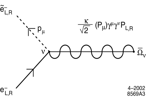
Figure 1: Feynman rule for the gravitino, fermion, scalar coupling. $P_{L,R}$ represent the standard projection operators.

4 Phenomenological Analysis and Numerical Results

We are now ready to apply our results to a phenomenological analysis. For purposes of illustration we focus on selectron pair production in high energy polarized $e^{+}e^{-}$ collisions. As discussed in the introduction, this process provides a valuable tool within the MSSM for determining the composition of the mixed neutralino states, $\tilde{\chi}^{0}_{i}$ in terms of the various pure SU(2) and U(1) wino and bino components, $\tilde{W}^{0}$, $\tilde{B}^{0}$. Here, we investigate how the existence of supersymmetric extra dimensions modifies this reaction.

The tree level processes contributing to selectron pair production in the presence of a supersymmetric bulk are presented in Fig. 2. In addition to the standard $\gamma,Z$ s-channel exchange and $\tilde{B}^{0},\tilde{W}^{0}$ t-channel contributions present in the MSSM, we now have contributions arising from the s-channel exchange of the bulk graviton KK tower and the t-channel exchange of the bulk gravitino KK tower. There are no u-channel contributions due to the non-identical final states. The contributions from neutral higgsino states are negligible due to the smallness of the Yukawa coupling. The diagrammatic contributions to the individual scattering processes for left- and right-handed selectron production with initial polarized electron beams are summarized in Table 1. Note that the $\tilde{W}^{0}$ exchange only contributes to the process $e^{-}_{L}e^{+}\rightarrow\tilde{e}_{L}^{-}\tilde{e}_{L}^{+}$, and that the t-channel gravitino and the $\tilde{B}^{0}$ contributions are isolated in the reaction $e^{-}_{L,R}e^{+}\rightarrow\tilde{e}^{-}_{L,R}\tilde{e}^{+}_{R,L}$.

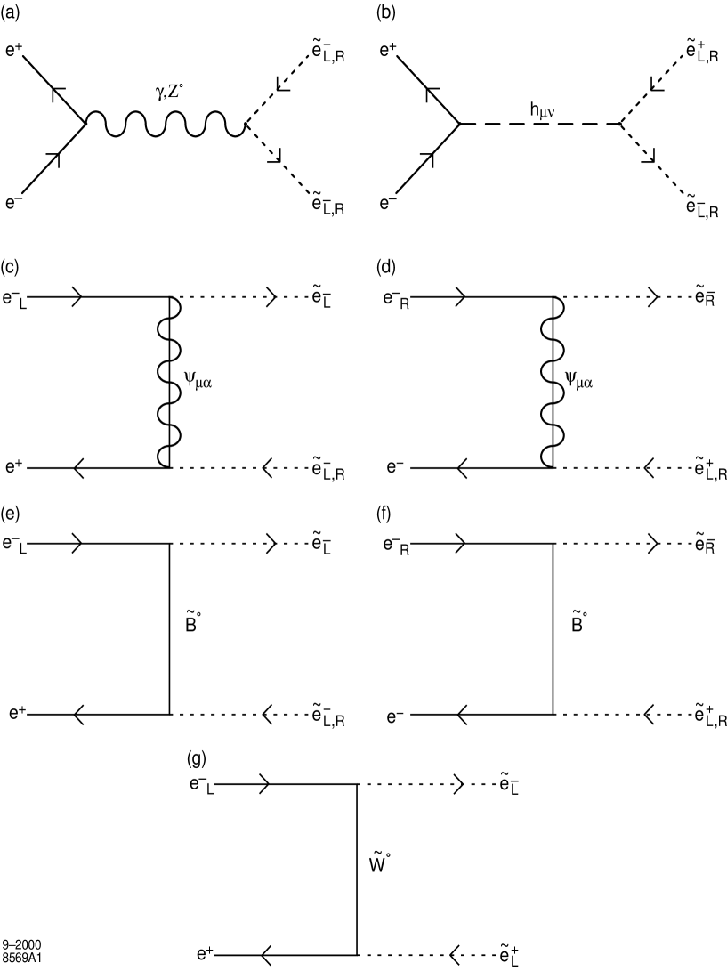
Figure 2: Processes contributing to scalar electron pair production in polarized $e^{+}e^{-}$ collisions. The state $h_{\mu\nu}$ represents the bulk graviton KK tower, $\Psi_{\mu\alpha}$ the bulk gravitino KK tower, and $\tilde{B}^{0},\,\tilde{W}^{0}$ correspond to the unmixed MSSM gaugino states.

	$\tilde{e}^{-}_{L}\tilde{e}^{+}_{L}$	$\tilde{e}^{-}_{R}\tilde{e}^{+}_{L}$	$\tilde{e}^{-}_{L}\tilde{e}^{+}_{R}$	$\tilde{e}^{-}_{R}\tilde{e}^{+}_{R}$
$e^{-}_{L}e^{+}$	s-channel $\gamma\,,Z\,,G_{n}$			s-channel $\gamma\,,Z\,,G_{n}$
	t-channel $\tilde{W}\,,\tilde{B}\,,\Psi_{n}$		t-channel $\tilde{B}\,,\Psi_{n}$
$e^{-}_{R}e^{+}$	s-channel $\gamma\,,Z\,,G_{n}$			s-channel $\gamma\,,Z\,,G_{n}$
		t-channel $\tilde{B}\,,\Psi_{n}$		t-channel $\tilde{B}\,,\Psi_{n}$

Table 1: The diagrammatic contributions to individual scattering processes for polarized electron beams. A blank box indicates that there are no contributions for that polarization configuration.

Our amplitudes for the standard MSSM contributions to the reaction $e^{-}(p_{2})e^{+}(p_{1})\rightarrow\tilde{e}^{-}(k_{2})\tilde{e}^{+}(k_{1})$ (with the direction of the charge flow as indicated in Fig. 2) reproduce the results in [23]. The unpolarized matrix element for the case of massive gravitino KK exchanges is

$${\cal M}={\frac{\kappa^{2}}{2}}\sum_{\vec{n}}{\frac{k_{1}^{\nu}k_{2}^{\rho}}{t-m^{2}_{\vec{n}}}}\bar{e}(p_{1})\gamma_{\mu}\gamma_{\nu}P^{\vec{n},\mu\tau}\gamma_{\rho}\gamma_{\tau}e(p_{2})\,,$$ (48)

where the sum extends over the gravitino KK modes and we recall that $\kappa=\sqrt{8\pi G_{N}}=\bar{M}_{P}^{-1}$ is the reduced Planck scale. $P^{\vec{n},\mu\tau}$ represents the numerator of the propagator for a Rarita-Schwinger field of mass $m_{\vec{n}}$ and is given in Appendix B. The mass splitting between the evenly spaced bulk gravitino KK excitations is given by $1/R_{c}$, which lies in the range $10^{-4}$ eV to few MeV for $\delta=2$ to 6 assuming $M_{D}\sim 1$ TeV; their number density is thus large at collider energies. The sum over the KK states can then be approximated by an integral which is log divergent for $\delta=2$ and power divergent for $\delta>2$. We employ a cut-off to regulate these ultraviolet divergences, with the cut-off being set to $\Lambda_{c}$, which in general is different from $M_{D}$, to account for the uncertainties from the unknown ultraviolet physics. This approach is the most model independent and is that generally used in the case of virtual graviton exchange [9]. In practice, the integral over the gravitino KK states is more complicated than that in the case with spin-2 gravitons due to the dependence of the gravitino propagator on $m_{\vec{n}}$. We find that the leading order term for $\sqrt{|t|}\ll\Lambda_{c}$ results in the replacement (in the case of $\delta=6$)

$${\frac{\kappa^{2}}{2}}\sum_{\vec{n}}{\frac{P^{\vec{n},\mu\tau}}{t-m^{2}_{\vec{n}}}}\rightarrow{\frac{-i8\pi}{5\Lambda_{c}^{3}}}\left(\eta^{\mu\nu}-{\frac{1}{3}}\gamma^{\mu}\gamma^{\nu}\right)\,$$ (49)

in the matrix element; the structure of the summed gravitino propagator is thus altered from that of a single massive state. Hence the leading order behavior for gravitino KK exchange results in a dimension-6 operator! This is in stark contrast to graviton KK exchange which yields a dimension-8 operator at leading order. We thus expect an increased sensitivity to the fundamental scale $M_{D}$ in the case of a supersymmetric bulk. Our derivation of the summation over the bulk gravitino KK states in the matrix element is detailed in Appendix C. Lastly, the bulk graviton KK tower contributes an additional amplitude of the form [24]

$${\cal M}={\frac{2}{\Lambda_{c}^{4}}}(t-u)(k_{1}-k_{2})_{\mu}\bar{e}(p_{2})\gamma^{\mu}e(p_{1})\,.$$ (50)

In order to perform a numerical analysis of this process, we need to specify a concrete supersymmetric model. We choose that of Gauge Mediated Supersymmetry Breaking (GSMB) as it naturally contains a light zero-mode gravitino. We specify a sample set of input parameters at the messenger scale, where the supersymmetry breaking is mediated via the messenger sector, and use the Renormalization Group Equations (RGE) to obtain the low-energy sparticle spectrum. We choose two sets of sample input parameters describing the messenger sector which are consistent with our model. The RGE evolution of these parameter sets is performed in ISAJET v7.51 [40] and results in the sparticle spectrum

$${\rm Set~{}I}: m_{\tilde{e}_{L}} =217.0\,{\rm GeV},\quad m_{\tilde{e}_{R}}=108.0\,{\rm GeV},\quad\chi^{0}_{i}=(76.5,\,141.5,\,337.0,\,367.0)\,{\rm GeV}\,,$$

$${\rm Set~{}II}: m_{\tilde{e}_{L}} =210.5\,{\rm GeV},\quad m_{\tilde{e}_{R}}=104.5\,{\rm GeV},\quad\chi^{0}_{i}=(110.5,\,209.6,\,322.5,\,324.0)\,{\rm GeV}\,,$$

where $\chi^{0}_{i}$ with $i=1,4$ corresponds to the four mixed neutralino states. The first set of parameters yields a bino-like state for the lightest neutralino, whereas the second set results in a Higgsino-like state for $\chi^{0}_{1}$. These two sets are chosen so we can investigate the dependence of the kinematic distributions on the composition of the lightest neutralino state. Note that the $\tilde{e}_{L}$ and $\tilde{e}_{R}$ masses are essentially equivalent between the two sets and hence will not induce any kinematical differences in the distributions. In addition, these input parameters were selected in order to obtain a sparticle spectrum which is kinematically accessible to the Linear Collider; our results are essentially insensitive to the exact details of the spectrum. We stress that our analysis is purely phenomenological and that our conclusions do not depend on the physics inherent to GMSB. Except where noted, we perform our numerical analysis for the case of $\delta=6$, following our above discussion of supergravity models. From here on, we refer to these two spectra as our $D=4$ supersymmetric models.

It is instructive to first examine the effects of each class of contributions to selectron pair production. This is displayed in Fig 3, which shows the angular distribution for the process $e^{-}_{R}e^{+}\rightarrow\tilde{e}_{R}^{+}\tilde{e}_{R}^{-}$ with $\sqrt{s}=500$ GeV assuming 100% polarization of the electron beam; we show this particular reaction merely for purposes of demonstration. The bottom curve represents the full contributions (s- and t-channel) from the 4-dimensional standard gauge-mediated supersymmetric model discussed above in the case where the $\chi^{0}_{1}$ is bino-like, corresponding to parameter set I. Our numerical results for the MSSM case agree with those in the literature [23]. The middle curve displays the effects of adding only the s-channel contributions of the bulk graviton KK tower in the scenario of a non-supersymmetric bulk with $\Lambda_{c}=1.5$ TeV. We see that there is little difference in the distribution between the $D=4$ supersymmetric case and with the addition of the graviton KK tower, in either shape or magnitude. It would hence be difficult to disentangle the effects of graviton exchange from an accurate measurement of the underlying supersymmetric parameters using this process alone. The top curve corresponds to the full set of contributions from a supersymmetric bulk, i.e., our standard supersymmetric model plus KK graviton and KK gravitino tower exchange for the case of six extra dimensions with $\Lambda_{c}=1.5$ TeV. Here we see that the exchange of bulk gravitino KK states yields a large enhancement in the cross section and a substantial shift in the shape of the angular distribution, particularly at forward angles, even for $\Lambda_{c}=3\sqrt{s}$. This provides a dramatic signal for a supersymmetric bulk!

In Fig. 4 we explore the modifications to the angular distribution for $e^{-}_{R}e^{+}\rightarrow\tilde{e}_{R}^{+}\tilde{e}_{R}^{-}$ from a supersymmetric bulk as the value of $\delta$ changes, using our parameter set I for demonstration. In principle there are two competing effects which may modify the distributions: (i) the number of degenerate gravitinos in each KK level as a result of the reduction of fermions, versus (ii) the volume factor that appears in the density of states in the integral over the gravitino propagator which sums over the states in the KK tower, and its dependence on $\Lambda_{c}$. As discussed above, the number of degenerate gravitinos is reduced as the number of extra dimensions decreases; this results in a reduction of the cross section in the general case of extended low-energy supersymmetries. However, this effect does not modify our analysis since we have assumed the $N=1$ at low-energy. The second effect arises from the increase in $R_{c}$, with $\Lambda_{c}$ being held fixed, for smaller values of $\delta$ as can be seen in Appendix C. This volume factor arises in the integral over the propagators for the bulk gravitino KK tower and is discussed in Appendix C. In this figure, we compare the event rates for this process for the cases $\delta=2$ and 6, corresponding to the top and bottom curves, respectively. We note that the shape of the distribution differs in the two cases due to the form of the sub-leading terms in the integral over the propagator of the KK states. For the remainder of our analysis, we will display results only for the more conservative case of $\delta=6$.

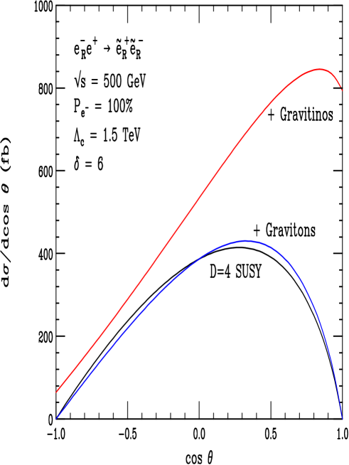
Figure 3: The angular distribution for $e^{-}_{R}e^{+}\rightarrow\tilde{e}_{R}^{+}\tilde{e}_{R}^{-}$ from the $D=4$ supersymmetric model I, plus the addition of bulk graviton KK tower exchange, and with bulk gravitino KK tower exchange, corresponding to the bottom, middle, and top curves, respectively.

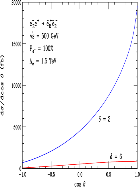
Figure 4: A comparison of the event rates for the cases with $\delta=2$ and 6, corresponding to the top and bottom curves, respectively.

Let us now study the variations in the distributions between the two different compositions of the lightest neutralino. Figure 5 shows the angular distributions with $100\%$ electron beam polarization for each helicity configuration listed in Table 1 for the two sets of parameters discussed above, with and without the contributions from supersymmetric extra dimensions. In each case, the solid curve corresponds to the bino-like case and the dashed curve represents the Higgsino-like scenario. The top set of curves are those for a supersymmetric bulk with $\Lambda_{c}=1.5$ TeV, while the bottom set corresponds to our two $D=4$ supersymmetric models, i.e., without the graviton and gravitino KK contributions. We note that the $D=4$ results agree with those in the literature [23]. We see from the figure that in the process where the gravitino contributions are dominant, $e^{-}_{L,R}e^{+}\rightarrow\tilde{e}_{L}^{\pm}\tilde{e}_{R}^{\mp}$, there is little difference in the shape or magnitude between the two $\chi^{0}_{1}$ compositions. The use of selectron pair production in polarized $e^{+}e^{-}$ collisions as a means of determining the composition of the lightest neutralino is thus made more difficult in the scenario with supersymmetric large extra dimensions. In what follows, we present results only for the bino-like $\chi^{0}_{1}$ as a sample case; our conclusions will not be dependent on the assumptions of the composition of the lightest neutralino.

     

     

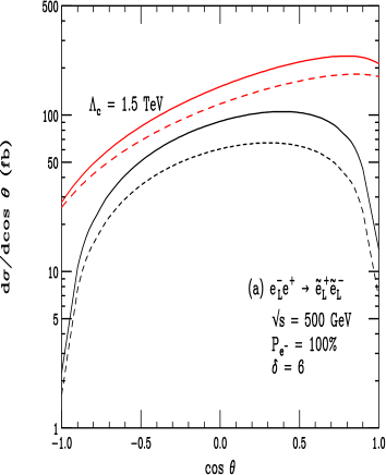
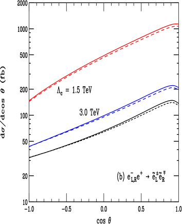
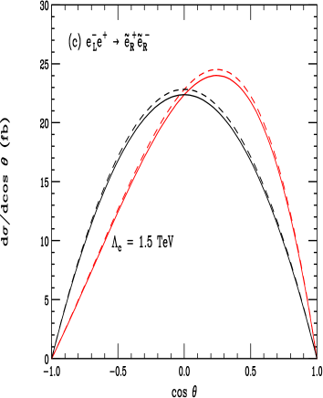
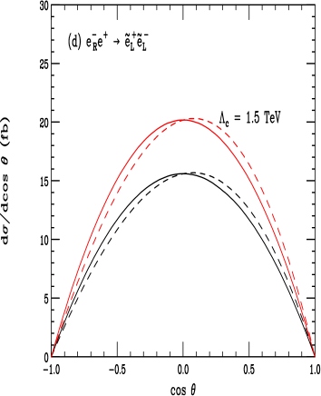
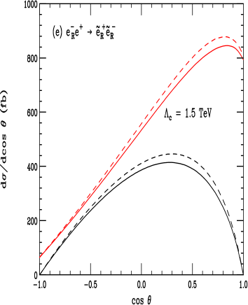
Figure 5: Angular distributions for each helicity configuration with supersymmetric bulk contributions for $\Lambda_{c}=1.5$ TeV (top curves), and for the $D=4$ supersymmetric models (bottom curves). The solid (dashed) curves correspond to a bino-like (Higgsino-like) composition of the lightest neutralino.

We now examine in Fig. 6 the total cross section as a function of center-of-mass energy for each helicity configuration. In each case, the bottom curve represents the $D=4$ bino-like supersymmetric model, while the remaining curves, from top to bottom, are for a supersymmetric bulk with $\Lambda_{c}=1.5,3.0,6.0$ TeV. In some reactions, the results for $\Lambda_{c}=6.0$ TeV are indistinguishable from the $D=4$ case. Here we can see the effects of unitarity violation as $\sqrt{s}$ approaches the value of the cut-off scale. Clearly, the new, as of yet unknown, ultra-violet physics will set-in at this point to regularize the cross section.

     

     

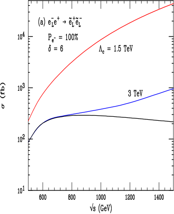
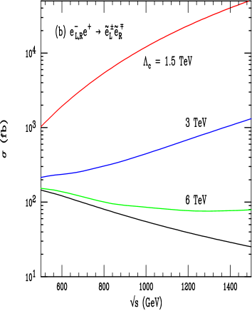
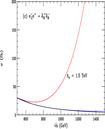
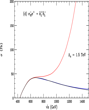
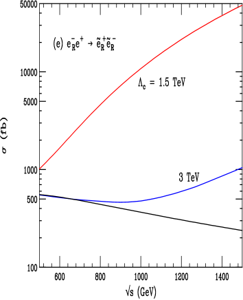
Figure 6: Total cross sections as a function of center of mass energy. The bottom curve corresponds to the $D=4$ supersymmetric model, and the other curves are for a $\delta=6$ supersymmetric bulk with the cut-off as labeled. In figures (c) and (d), the $\Lambda_{c}=3$ TeV curve is barely distinguishable from that for the case of $D=4$ supersymmetry.

Next, we present in Fig. 7 and 8 the number of events for the binned angular distribution for each helicity configuration with $80\%$ polarized electron beams for $\sqrt{s}=500$ GeV and $500{\rm fb}^{-1}$ of integrated luminosity. In each case, the solid histogram corresponds to the $D=4$ bino-like supersymmetric model, while the “data” points represent the addition of the bulk graviton and gravitino KK tower exchange for $\Lambda_{c}=1.5,3.0,6.0$ TeV from top to bottom. As before, the contributions with $\Lambda_{c}=6.0$ TeV are only distinguishable from the $D=4$ results in the case of $e^{-}_{L,R}e^{+}\rightarrow\tilde{e}_{L}^{\pm}\tilde{e}_{R}^{\mp}$. The error bars on the “data” points are statistical only. We see that in most of the reactions, the case of $\Lambda=3.0$ TeV leads to only a slight increase in event rate in each bin, whereas for $e^{-}_{L,R}e^{+}\rightarrow\tilde{e}_{L}^{\pm}\tilde{e}_{R}^{\mp}$, the t-channel bulk gravitino KK exchange is significant, leading to observable deviations from the $D=4$ case even for $\Lambda_{c}=6.0$ TeV.

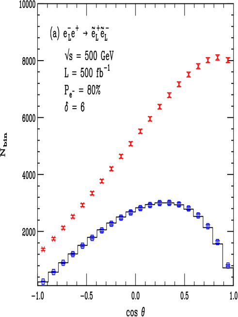
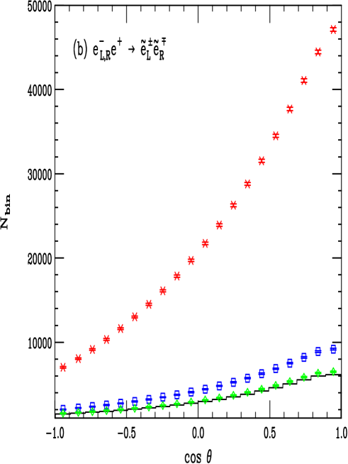
Figure 7: (a-b) Polarized binned angular distributions for each helicity configuration, taking an 80% polarization of the initial electron beam. The solid histogram represents the $D=4$ bino-like model, while the “data” points correspond to the effects of a supersymmetric bulk with $\Lambda_{c}=1.5,3.0,6.0$ TeV from top to bottom. The $\Lambda_{c}=6.0$ TeV case is only discernable in Figure (b).

     

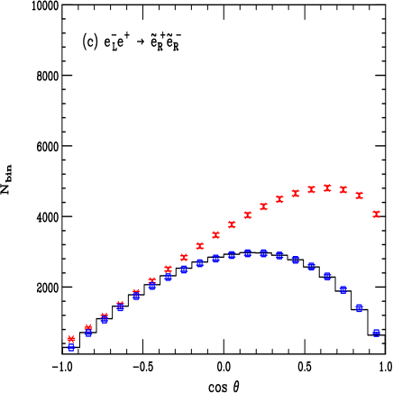
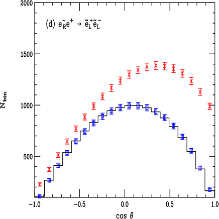
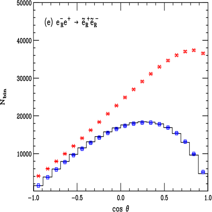
Figure 8: (c-e) Polarized binned angular distributions for each helicity configuration, taking an 80% polarization of the initial electron beam. The solid histogram represents the $D=4$ bino-like model, while the “data” points correspond to the effects of a supersymmetric bulk with $\Lambda_{c}=1.5,3.0,6.0$ TeV from top to bottom.

An interesting polarization asymmetry can be defined for the case of $\tilde{e}_{L}^{+}\tilde{e}_{L}^{-}$ and $\tilde{e}_{R}^{+}\tilde{e}_{R}^{-}$ production. It is given by

$$A_{\rm pol}={d\sigma_{L}-d\sigma_{R}\over d\sigma_{L}+d\sigma_{R}}\,,$$ (51)

where the left- and right-handed subscripts refer to the polarization of the initial electron beam, i.e., $d\sigma_{i}=d\sigma(e^{-}_{i}e^{+}\rightarrow\tilde{e}_{L}^{-}\tilde{e}_{L}^{+}\,,\tilde{e}_{R}^{-}\tilde{e}_{R}^{+})/d\cos\theta$. This asymmetry is displayed in Fig. 9, where the solid histogram again represents our $D=4$ bino-like supersymmetric model and the “data” points are for a supersymmetric bulk with $\Lambda_{c}=1.5$ and 3.0 TeV. The error bars are again statistical only and assume an integrated luminosity of 500 ${\rm fb}^{-1}$. The electron beam polarization is taken to be 80%. We see that the asymmetry varies substantially from its $D=4$ value with the addition of gravitino KK exchange, thus providing an additional signal for a supersymmetric bulk.

     

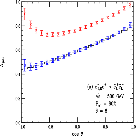
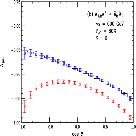
Figure 9: Polarization asymmetry defined in the text binned in $\cos\theta$. The solid histogram represents the $D=4$ bino-like model, while the two sets of “data” points include the contributions from supersymmetric bulk with $\Lambda_{c}=1.5$ and 3.0 TeV.

We now compute the potential sensitivity to the cut-off scale from selectron pair production using our sample case with a bino-like lightest neutralino state for purposes of demonstration. We employ the usual $\chi^{2}$ procedure, taking

$$\chi^{2}=\sum_{\rm bins}\left[{\left({\frac{d\sigma}{d\cos\theta}}\right)_{4d}-\left({\frac{d\sigma}{d\cos\theta}}\right)_{10d}\over\delta\left({\frac{d\sigma}{d\cos\theta}}\right)}\right]^{2}\,,$$ (52)

where we include statistical errors only. We sum over both initial left- and right-handed electron polarization states, assuming $P_{e^{-}}=80\%$. The resulting 95% C.L. search for $\Lambda_{c}$ from each final state, $\tilde{e}_{L}^{+}\tilde{e}_{L}^{-}\,,\tilde{e}_{R}^{+}\tilde{e}_{R}^{-}$, and $\tilde{e}_{L}^{\pm}\tilde{e}_{R}^{\mp}$, is given as a function of integrated luminosity in Fig. 10 for $\sqrt{s}=0.5$ and 1.0 TeV. We see that for 500 ${\rm fb}^{-1}$ of integrated luminosity, corresponding to design values, the search reach in the left- and right-handed selectron pair production channels is given roughly by $\Lambda_{c}\simeq 6-10\times\sqrt{s}$, which is essentially what is achievable for bulk graviton KK exchange in the reaction $e^{+}e^{-}\rightarrow f\bar{f}$ [9]. However, the $\tilde{e}_{L}^{\pm}\tilde{e}_{R}^{\mp}$ production channel yields an enormous search capability with a 95% C.L. sensitivity to $\Lambda_{c}$ of order $25\times\sqrt{s}$ for design luminosity. This process thus has the potential to either discover a supersymmetric bulk, or eliminate the possibility of supersymmetric large extra dimensions as being relevant to the hierarchy problem. We stress that there is nothing special about our choice of supersymmetric parameters; our results will hold as long as selectrons are kinematically accessible to high energy $e^{+}e^{-}$ colliders. We conclude that selectron pair production provides a very powerful tool in searching for a supersymmetric bulk.

     

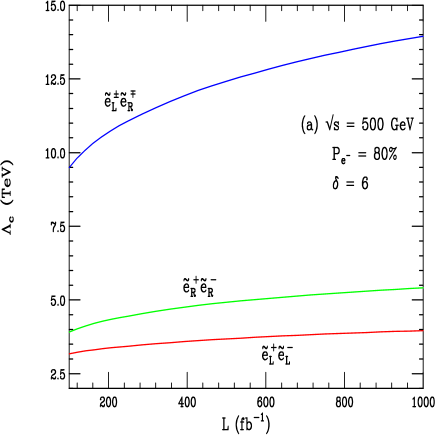
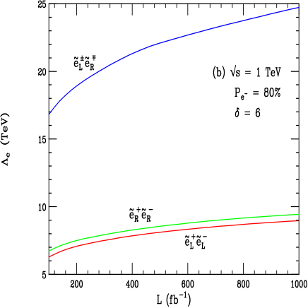
Figure 10: 95% C.L. search reach for $\Lambda_{c}$ in each production channel as a function of integrated luminosity for $\sqrt{s}=0.5$ and 1.0 TeV.

5 Conclusions

In summary, we have examined the phenomenological consequences of a supersymmetric bulk in the scenario of large extra dimensions. We assumed that supersymmetry is unbroken in the bulk, with gravitons and gravitinos being free to propagate throughout the higher dimensional space, and that the SM and MSSM gauge and matter fields are confined to a 3-brane. Motivated by string theory, we worked in the framework of $D=10$ supergravity, and found that the KK reduction of the bulk gravitinos yields four Majorana spinors in four dimensions. We then assumed that the residual $N=4$ supersymmetry is broken near the fundamental scale $M_{D}$, with only $N=1$ supersymmetry surviving at the electroweak scale.

Starting with the $D=10$ action for this scenario, we expanded the bulk gravitino into a KK tower of states, and determined the field equation obeyed by the spin-3/2 KK excitations. We then derived the coupling of the bulk gravitino KK states to fermions and their scalar partners on the brane. We applied these results to a phenomenological analysis by examining the effects of virtual exchange of the gravitino KK tower in superparticle pair production. We focused on the reaction $e^{+}e^{-}\rightarrow\tilde{e}^{+}\tilde{e}^{-}$ as this process is a benchmark for collider supersymmetry studies. Our numerical analysis was performed in the framework of gauge mediated supersymmetry breaking as it naturally affords a light zero-mode gravitino. However, our results do not depend on the specifics of this particular model, with the exception of the existence of a light zero-mode gravitino state.

Performing the sum over the KK propagators, we found that the leading order contribution to this process arises from a dimension-6 operator, and is independent of the zero-mode mass. This is in stark contrast to the virtual exchange of spin-2 graviton KK states, which yields a dimension-8 operator at leading order. We thus found that the gravitino KK contributions substantially alter the production rates and angular distributions for selectron pair production, and may essentially be isolated in the $\tilde{e}_{L}^{\pm}\tilde{e}_{R}^{\mp}$ channel. The resulting sensitivity to the cut-off scale is tremendous, being of order $20-25\times\sqrt{s}$.

We expect that the virtual exchange of gravitino KK states in hadronic collisions will have somewhat less of an effect in squark and gluino pair production than what we have found here. The reason is that these processes are initiated by both quark annihilation and gluon fusion sub-processes, only one of which will be sensitive to tree-level gravitino exchange for a given production channel. The sensitivity to the cut-off scale will then depend on the relative weighting of the quark and gluon initial states. In addition, t-channel gravitino contributions will only be numerically relevant for up- and down-squark production due to flavor conservation; hence their effect will be diluted by the production of the other degenerate squark flavors and the relative weighting of the parton densities.

Lastly, we note that virtual exchange of gravitino KK states may also have a large effect on selectron pair production in $e^{-}e^{-}$ collisions, which are tailor-made for t-channel Majorana exchanges. High energy Linear Colliders thus provide an excellent probe for the existence of supersymmetric large extra dimensions, and have the capability of discovering this possibility or eliminating it as being relevant to the hierarchy problem.

6 Acknowledgments

The authors would like to acknowledge useful discussions with Hooman Davoudiasl, David London, Maxim Perelstein, Michael Peskin, Frank Petriello, and Tom Rizzo.

Appendix A Representation of the Dirac Algebra

A convenient representation of the Dirac algebra, which simplifies the Kaluza-Klein decomposition, can be given in the $10$ dimensional space-time as follows,

$$\Gamma^{\mu}\> = \>\gamma^{\mu}\>\otimes\>1_{2}\otimes 1_{4}\,,$$

$$\Gamma^{3+(2j-1)}\> = \>\gamma^{5}\>\otimes\>\sigma_{1}\>\otimes\>\alpha_{j}\,,$$ (53)

$$\Gamma^{3+(2j)}\> = \>\gamma^{5}\>\otimes\>\sigma_{3}\>\otimes\>\beta_{j}\,,$$

where the $\gamma^{\mu}$ are standard $4$ dimensional Dirac matrices, $i,j=1,2,3$ and $\mu=0,\ldots,3$. Here $\alpha$ and $\beta$ are $4\times 4$ matrices satisfying

$$\{\alpha_{i},\alpha_{j}\}\> =\>\{\beta_{i},\beta_{j}\}\>=\>-2\delta^{ij}\,,$$

$$\{\alpha_{i},\beta_{j}\}\> =\>0\,,$$ (54a)

and the $\sigma$’s are standard pauli matrices satisfying

$$\sigma^{i}\sigma^{j}\>=\>\delta^{ij}\>+\>i\epsilon^{ijk}\sigma^{k}\,,$$ (55)

and $\gamma^{5}$ anticommutes with the $\gamma^{\mu}$

$$\{\gamma^{\mu},\gamma^{5}\}\>=\>0\,.$$ (56)

The $\alpha$ and $\beta$ matrices can be represented as follows [41]

$$\alpha_{1}\> =\>\left(\begin{matrix}0&\sigma_{1}\\ -\sigma_{1}&0\end{matrix}\right)\,, \alpha_{2}\> =\>\left(\begin{matrix}0&-\sigma_{3}\\ \sigma_{3}&0\end{matrix}\right)\,, \alpha_{3}\> =\>\left(\begin{matrix}i\sigma_{2}&0\\ 0&i\sigma{2}\end{matrix}\right)\,,$$ (57a)

$$\beta_{1}\> =\>\left(\begin{matrix}0&-i\sigma_{2}\\ -i\sigma_{2}&0\end{matrix}\right)\,, \beta_{2}\> =\>\left(\begin{matrix}0&-1\\ 1&0\end{matrix}\right)\,, \beta_{3}\> =\>\left(\begin{matrix}i\sigma_{2}&0\\ 0&-i\sigma{2}\end{matrix}\right)\,.$$ (57b)

This representation of the Gamma matrices makes manifest the decomposition to four dimensions, since $\Gamma^{\mu}$ for $\mu=0,\ldots,3$ is the tensor product of four dimensional Gamma matrices with an $8\times 8$ identity acting on an internal index. With these conventions, the space-like Gamma matrices are anti-hermitian, while the time-like Gamma matrix is hermitian.

Appendix B Propagator for a Single Massive KK State

To find the propagator for a single massive Kaluza-Klein state, we invert the kinetic piece of the operator appearing in (33). We solve

$$\hat{O}^{\vec{n},\mu\nu}\>P^{\vec{n}}_{\nu\sigma}\>=\>i\>(k^{2}-m_{\vec{n}}^{2})\>\delta^{\mu}_{\sigma}$$ (58)

for $P^{\vec{n}}_{\nu\sigma}$, where $\hat{O}^{\vec{n},\mu\nu}$ is obtained by writing the Lagrangian for a single Kaluza-Klein state in (33) as

$$\mathcal{L}^{\vec{n}}\>=\>\frac{1}{2}\bar{\Psi}_{\mu}\>\hat{O}^{\vec{n},\mu\nu}\>\Psi_{\nu}\,.$$ (59)

The propagator for the mode specified by the vector of integers $\vec{n}$ is then given by

$$\frac{P^{\vec{n}}_{\mu\nu}}{k^{2}-m_{\vec{n}}^{2}+i\epsilon}\,.$$ (60)

We are free to drop the $i\epsilon$ convergence term as we are interested in computing t-channel diagrams for which $t<0$, and so no poles are encountered. To solve (58), we expand $P^{\vec{n}}_{\mu\nu}$ as a linear combination of the standard set of sixteen $4\times 4$ matrices formed from antisymmetrized combinations of the gamma matrices $\{1,\gamma^{\mu},\sigma^{\mu\nu},\gamma^{\mu}\gamma^{5},\gamma^{5}\}$, which form a basis for complex $4\times 4$ matrices, together with $\{\eta_{\mu\nu},k_{\mu},k_{\nu}\}$, to generate the correct tensor structure. We then solve for the coefficients in this expansion. The result is

$$P^{\vec{n},\mu\nu}\>=\>i\>\left(\not\!{k}+m_{\vec{n}}\right)\left(\frac{k^{\mu}k^{\nu}}{m_{\vec{n}}^{2}}-\eta^{\mu\nu}\right)-\frac{i}{3}\left(\gamma^{\mu}+\frac{k^{\mu}}{m_{\vec{n}}}\right)\left(\not\!{k}-m_{\vec{n}}\right)\left(\gamma^{\nu}+\frac{k^{\nu}}{m_{\vec{n}}}\right)$$ (61)

and satisfies (on-shell) the standard condition $k_{\mu}P^{\mu\nu}=0$ together with $\gamma_{\mu}P^{\mu\nu}=0$ which projects out the spin $\frac{1}{2}$ components.

Appendix C Summation of Kaluza-Klein States

The summation over the Kaluza-Klein states contributing to the propagator for the exchange of a virtual gravitino KK tower is inherently more complicated than in the case of spin-$2$ exchange, and leads to a quantitatively different result. In addition, we must also include the effects of the finite mass of the zero-mode gravitino, $m_{0}$ [42]. We state here the basic result to leading order in the cut-off $\Lambda_{c}$ for the case when $\Lambda_{c}^{2}\gg|t|,m_{0}^{2}$, and $\delta=6$ extra dimensions, which is the example considered in the text. The result is easily generalized to other values of $\delta$.

The mass difference between neighboring KK states, $|\Delta m|\sim 1/R_{c}$, is much smaller than the cut-off ($|\Delta m|\ll\Lambda_{c}$) leading to a large number of states to be summed over. The mass of the individual KK state is given by (31)

$$m^{2}_{\vec{n}}\>=\>\frac{\vec{n}\cdot\vec{n}}{R_{c}^{2}}\,,$$ (62)

where $R_{c}$ is the common compactification radius. The near degeneracy of the KK state masses allows us to treat the discrete population of states on the lattice labeled by the vector $\vec{n}=(n_{1},\ldots,n_{\delta})$ in the continuum limit. The number of KK states $dN$ in the thin shell between $m_{\vec{n}}^{2}$ and $m_{\vec{n}}^{2}+dm_{\vec{n}}^{2}$ is

$$dN\>=\>\rho(m_{\vec{n}}^{2})dm_{\vec{n}}^{2}\,,$$ (63)

with the density function

$$\rho(m_{\vec{n}}^{2})\>=\>\frac{(2\pi R_{c})^{\delta}(m_{\vec{n}}^{2}-m_{0}^{2})^{\frac{\delta-2}{2}}}{(4\pi)^{\frac{\delta}{2}}\Gamma({\frac{\delta}{2}})}\,.$$ (64)

The coherent sum over these states is at the amplitude level and involves terms of the form

$$D_{\sigma}(t)\>\approx\>-i\>\int_{m_{0}^{2}}^{\Lambda_{c}^{2}}\>dm_{\vec{n}}^{2}\>\rho(m_{\vec{n}}^{2})\frac{F_{\sigma,\vec{n}}}{|t|+m_{\vec{n}}^{2}}\,,$$ (65)

where the momentum exchange is in the t-channel with $t<0$. Here, we have included an explicit ultraviolet cut-off $\Lambda_{c}$ in order to regulate this divergent integral. As can be seen in Appendix B, in the case of the gravitino propagator there are four distinct classes of $F_{\alpha,\vec{n}}$ to consider, given by

$$F_{\sigma,\vec{n}}\>=\>|m_{\vec{n}}|^{\sigma-2}\,,$$ (66)

with $\sigma=0,1,2,3$. Using (62), (66) and the change of variables $y=m_{\vec{n}}/\chi$, with $\chi\equiv\sqrt{|t|}$, the integral (65) can be put in the form

$$D_{\sigma}(t)\>\approx\>\frac{-2i(2\pi R_{c})^{\delta}\chi^{\sigma+\delta-4}}{(4\pi)^{\frac{\delta}{2}}\Gamma(\frac{\delta}{2})}\>\int_{m_{0}/\chi}^{\Lambda_{c}/\chi}\>dy\>\frac{(y^{2}-\frac{m_{0}^{2}}{\chi^{2}})^{\frac{\delta-2}{2}}y^{\sigma-1}}{1+y^{2}}\,.$$ (67)

This integral can be evaluated by making use of Appell’s hypergeometric function
$F_{1}(a;b_{1},b_{2};c;z_{1},z_{2})$ which generalizes hypergeometric series to two variables [43]. It has the one dimensional integral representation

$$\frac{\Gamma(a)\Gamma(c-a)}{\Gamma(c)}\>F_{1}(a;b_{1},b_{2};c;z_{1},z_{2})\>=\>\\ \int_{0}^{1}\>u^{a-1}(1-u)^{c-a-1}(1-uz_{1})^{-b1}(1-uz_{2})^{-b2}\>du\,,$$ (68)

and the series expansion

$$F_{1}(a;b_{1},b_{2};c;z_{1},z_{2})\>=\>\sum_{m=0}^{\infty}\>\sum_{n=0}^{\infty}\>\frac{(a)_{m+n}(b1)_{m}(b2)_{n}}{m!n!(c)_{m+n}}\>z_{1}^{m}\>z_{2}^{n}\,,$$ (69)

where $(a)_{n}$ is the Pochhammer symbol defined as

$$(a)_{n}\>=\>a(a+1)\ldots(a+n-1)\,.$$ (70)

For $\delta=6$ extra dimensions, the result to leading order in $\frac{\sqrt{|t|}}{\Lambda_{c}}\ll 1$ is

$$D_{\sigma}\>\approx\>\frac{-i\>\pi^{3}\>R_{c}^{6}\>\Lambda_{c}^{\sigma+2}}{\sigma+2}\,.$$ (71)

We note that at this order, the result is independent of the mass of the zero-mode, so long as this mass is much smaller than the cut-off scale. The results for the various values of $\sigma$ are explicitly listed in Table 2. For $\delta=2$ extra dimensions, the leading order result for $\sigma=3$ is

$$D_{\sigma=3}\>\approx\>-2i\pi R_{c}^{2}\>\Lambda_{c}\,.$$ (72)

We note that the behavior of the sub-leading terms for $\delta=2$ is quite different than that displayed in Table 2 for the case of $\delta=6$. We do not rely on the above approximations, but evaluate (67) numerically in our analysis.

$\sigma$	$i\>D_{\sigma}\>(\pi^{3}R_{c}^{6})^{-1}$
0	$\Lambda_{c}^{2}/2$
1	$\Lambda_{c}^{3}/3$
2	$\Lambda_{c}^{4}/4$
3	$\Lambda_{c}^{5}/5$

Table 2: Value of the integrals over the terms in the gravitino propagator in six extra dimensions.

An interesting feature of this result when applied to the gravitino propagator is that it modifies its qualitative structure, so that the summed propagator is dominated by a few terms. This gives rise to the following ($\sigma=3$) leading order behavior (for 6 extra dimensions)

$$\sum_{\vec{n}}P^{\vec{n},\mu\nu}\>\approx\>\frac{-i\pi^{3}\Lambda_{c}^{5}\>R_{c}^{6}}{5}\left(\eta^{\mu\nu}\>-\>\frac{1}{3}\gamma^{\mu}\gamma^{\nu}\right)\,.$$ (73)

Following Han et al., in [8], we take the relation between the compactification radius and the cut-off scale to be

$$R_{c}^{\delta}\>=\>\frac{8\sqrt{\pi^{(2-\delta)}}\>\Gamma(\frac{\delta}{2})}{\kappa^{2}\>\Lambda_{c}^{\delta+2}}\,,$$ (74)

with the gravitational coupling constant $\kappa=\sqrt{8\pi G_{N}}$.

References

- [1] N. Arkani-Hamed, S. Dimopoulos and G. R. Dvali, Phys. Lett. B 429, 263 (1998) [arXiv:hep-ph/9803315]; N. Arkani-Hamed, S. Dimopoulos and G. R. Dvali, Phys. Rev. D 59, 086004 (1999) [arXiv:hep-ph/9807344]; N. Arkani-Hamed, S. Dimopoulos and J. March-Russell, Phys. Rev. D 63, 064020 (2001) [arXiv:hep-th/9809124]; N. Arkani-Hamed, S. Dimopoulos, N. Kaloper and R. Sundrum, Phys. Lett. B 480, 193 (2000) [arXiv:hep-th/0001197].
- [2] I. Antoniadis, N. Arkani-Hamed, S. Dimopoulos and G. R. Dvali, Phys. Lett. B 436, 257 (1998) [arXiv:hep-ph/9804398].
- [3] N. Arkani-Hamed, S. Dimopoulos and J. March-Russell, Phys. Rev. D 63, 064020 (2001) [arXiv:hep-th/9809124].
- [4] E. Witten, Nucl. Phys. B 471, 135 (1996) [arXiv:hep-th/9602070]; J. D. Lykken, Phys. Rev. D 54, 3693 (1996) [arXiv:hep-th/9603133].
- [5] V. A. Rubakov and M. E. Shaposhnikov, Phys. Lett. B 125, 136 (1983).
- [6] P. Horava and E. Witten, Nucl. Phys. B 460, 506 (1996) [arXiv:hep-th/9510209], and Nucl. Phys. B 475, 94 (1996) [arXiv:hep-th/9603142].
- [7] J. Polchinski, arXiv:hep-th/9611050.
- [8] G. F. Giudice, R. Rattazzi and J. D. Wells, Nucl. Phys. B 544, 3 (1999) [arXiv:hep-ph/9811291]; T. Han, J. D. Lykken and R. J. Zhang, Phys. Rev. D 59, 105006 (1999) [arXiv:hep-ph/9811350]; E. A. Mirabelli, M. Perelstein and M. E. Peskin, Phys. Rev. Lett. 82, 2236 (1999) [arXiv:hep-ph/9811337]; K. Cheung and W. Y. Keung, Phys. Rev. D 60, 112003 (1999) [arXiv:hep-ph/9903294]; T. G. Rizzo, Phys. Rev. D 59, 115010 (1999) [arXiv:hep-ph/9901209], and arXiv:hep-ph/9910255; S. Cullen, M. Perelstein and M. E. Peskin, Phys. Rev. D 62, 055012 (2000) [arXiv:hep-ph/0001166].
- [9] J. L. Hewett, Phys. Rev. Lett. 82, 4765 (1999) [arXiv:hep-ph/9811356].
- [10] For a review of the experimental bounds from collider processes, see G. Landsberg, arXiv:hep-ex/0105039.
- [11] S. Cullen and M. Perelstein, Phys. Rev. Lett. 83, 268 (1999) [arXiv:hep-ph/9903422]; V. D. Barger, T. Han, C. Kao and R. J. Zhang, Phys. Lett. B 461, 34 (1999) [arXiv:hep-ph/9905474]; C. Hanhart, D. R. Phillips, S. Reddy and M. J. Savage, Nucl. Phys. B 595, 335 (2001) [arXiv:nucl-th/0007016]; L. J. Hall and D. R. Smith, Phys. Rev. D 60, 085008 (1999) [arXiv:hep-ph/9904267]; S. Hannestad and G. G. Raffelt, Phys. Rev. Lett. 88, 071301 (2002) [arXiv:hep-ph/0110067], and Phys. Rev. Lett. 88, 071301 (2002) [arXiv:hep-ph/0110067].
- [12] C. D. Hoyle, et al., Phys. Rev. Lett. 86, 1418 (2001) [arXiv:hep-ph/0011014]; E. G. Adelberger, arXiv:hep-ex/0202008.
- [13] Z. Chacko, M. A. Luty, A. E. Nelson and E. Ponton, JHEP 0001, 003 (2000) [arXiv:hep-ph/9911323]; D. E. Kaplan, G. D. Kribs and M. Schmaltz, Phys. Rev. D 62, 035010 (2000) [arXiv:hep-ph/9911293]; N. Arkani-Hamed, L. J. Hall, D. R. Smith and N. Weiner, Phys. Rev. D 63, 056003 (2001) [arXiv:hep-ph/9911421]; V. Di Clemente, S. F. King and D. A. Rayner, Nucl. Phys. B 617, 71 (2001) [arXiv:hep-ph/0107290]; D. E. Kaplan and T. M. Tait, JHEP 0006, 020 (2000) [arXiv:hep-ph/0004200]; Z. Chacko and M. A. Luty, arXiv:hep-ph/0112172.
- [14] E. A. Mirabelli and M. E. Peskin, Phys. Rev. D 58, 065002 (1998) [arXiv:hep-th/9712214]. For a general method of writing global supersymmetric Lagrangians in higher dimensions, including couplings to fields on the brane, see, N. Arkani-Hamed, T. Gregoire and J. Wacker, JHEP 0203, 055 (2002) [arXiv:hep-th/0101233].
- [15] C. Schmidhuber, Nucl. Phys. B 585, 385 (2000) [arXiv:hep-th/0005248], and Nucl. Phys. B 619, 603 (2001) [arXiv:hep-th/0104131].
- [16] R. Altendorfer, J. Bagger and D. Nemeschansky, Phys. Rev. D 63, 125025 (2001) [arXiv:hep-th/0003117]; J. Bagger, D. Nemeschansky and R. J. Zhang, JHEP 0108, 057 (2001) [arXiv:hep-th/0012163]; T. Gherghetta and A. Pomarol, Nucl. Phys. B 586, 141 (2000) [arXiv:hep-ph/0003129], and Nucl. Phys. B 602, 3 (2001) [arXiv:hep-ph/0012378].
- [17] D. Atwood, C. P. Burgess, E. Filotas, F. Leblond, D. London and I. Maksymyk, Phys. Rev. D 63, 025007 (2001) [arXiv:hep-ph/0007178].
- [18] P. Fayet, Phys. Lett. B 84, 421 (1979), and Phys. Lett. B 175, 471 (1986); D. A. Dicus, S. Nandi and J. Woodside, Phys. Rev. D 41, 2347 (1990), and Phys. Rev. D 43, 2951 (1991); D. A. Dicus and S. Nandi, Phys. Rev. D 56, 4166 (1997) [arXiv:hep-ph/9611312]; A. Brignole, F. Feruglio and F. Zwirner, Nucl. Phys. B 516, 13 (1998) [Erratum-ibid. B 555, 653 (1998)] [arXiv:hep-ph/9711516]; A. Brignole, F. Feruglio, M. L. Mangano and F. Zwirner, Nucl. Phys. B 526, 136 (1998) [Erratum-ibid. B 582, 759 (1998)] [arXiv:hep-ph/9801329]; S. Gopalakrishna and J. Wells, Phys. Lett. B 518, 123 (2001) [arXiv:hep-ph/0108006].
- [19] M. Nowakowski and S. D. Rindani, Phys. Lett. B 348, 115 (1995) [arXiv:hep-ph/9410262]; D. A. Dicus, R. N. Mohapatra and V. L. Teplitz, Phys. Rev. D 57, 578 (1998) [Erratum-ibid. D 57, 4496 (1998)] [arXiv:hep-ph/9708369]; M. Bolz, A. Brandenburg and W. Buchmuller, Nucl. Phys. B 606, 518 (2001) [arXiv:hep-ph/0012052].
- [20] T. Affolder et al. [CDF Collaboration], Phys. Rev. Lett. 85, 1378 (2000) [arXiv:hep-ex/0003026]; G. Abbiendi et al. [OPAL Collaboration], Phys. Lett. B 501, 12 (2001) [arXiv:hep-ex/0007014].
- [21] G. F. Giudice and R. Rattazzi, Phys. Rept. 322, 419 (1999) [arXiv:hep-ph/9801271]; S. Dimopoulos, M. Dine, S. Raby and S. Thomas, Phys. Rev. Lett. 76, 3494 (1996) [arXiv:hep-ph/9601367]; S. Ambrosanio, G. L. Kane, G. D. Kribs, S. P. Martin and S. Mrenna, Phys. Rev. D 54, 5395 (1996) [arXiv:hep-ph/9605398]; C. Kolda, Nucl. Phys. Proc. Suppl. 62, 266 (1998) [arXiv:hep-ph/9707450]; G. F. Giudice and R. Rattazzi, In *Kane, G.L. (ed.): Perspectives on supersymmetry* 355-377.
- [22] E. A. Baltz and H. Murayama, arXiv:astro-ph/0108172.
- [23] A. Bartl, H. Fraas and W. Majerotto, Z. Phys. C 34, 411 (1987); H. Baer, A. Bartl, D. Karatas, W. Majerotto and X. Tata, Int. J. Mod. Phys. A 4, 4111 (1989); T. Tsukamoto, K. Fujii, H. Murayama, M. Yamaguchi and Y. Okada, Phys. Rev. D 51, 3153 (1995).
- [24] T. G. Rizzo, Phys. Rev. D 60, 075001 (1999) [arXiv:hep-ph/9903475].
- [25] J. Polchinski, “String Theory. Vol. 1: An Introduction To The Bosonic String,”; “String Theory. Vol. 2: Superstring Theory And Beyond,”; Cambridge, UK: Univ. Pr. (1998) Vol. I 402 p; Vol. II 531 p.
- [26] D. Berenstein, V. Jejjala and R. G. Leigh, arXiv:hep-ph/0105042; I. Antoniadis, E. Kiritsis and T. Tomaras, Fortsch. Phys. 49 (2001) 573 [arXiv:hep-th/0111269]; L. E. Ibanez, arXiv:hep-ph/0109082.
- [27] P. Van Nieuwenhuizen, Phys. Rept. 68, 189 (1981); H. P. Nilles, Phys. Rept. 110, 1 (1984); D. Z. Freedman, in C78-08-23.107 ITP-SB-78-54 Session organizers report given at 19th Int. Conf. on High Energy Physics, Tokyo, Japan, Aug 23-30, 1978; M. J. Duff, B. E. Nilsson and C. N. Pope, Phys. Rept. 130, 1 (1986); D. Z. Freedman, P. van Nieuwenhuizen and S. Ferrara, in C76-10-06.18 ITP-SB-76-68 Invited talk given at Meeting of Div. of Particles and Fields of the APS, Brookhaven National Lab., Upton, N.Y., Oct 6-8, 1976.
- [28] D. Z. Freedman, P. van Nieuwenhuizen and S. Ferrara, Phys. Rev. D 13, 3214 (1976); S. Deser and B. Zumino, Phys. Lett. B 62, 335 (1976).
- [29] P. Van Nieuwenhuizen, Nucl. Phys. B 60 (1973) 478.
- [30] W. Rarita and J. S. Schwinger, Phys. Rev. 60 (1941) 61.
- [31] M. B. Green, J. H. Schwarz and E. Witten, “Superstring Theory. Vol. 1: Introduction,”; “Superstring Theory. Vol. 2: Loop Amplitudes, Anomalies And Phenomenology,”; Cambridge, Uk: Univ. Pr. (1987) Vol I, 469 p; Vol II 596 p. (Cambridge Monographs On Mathematical Physics).
- [32] A. Salam and J. Strathdee, Annals Phys. 141, 316 (1982).
- [33] N. D. Birrell and P. C. Davies, Cambridge, Uk: Univ. Pr. ( 1982) 340p.
- [34] S. Weinberg, “The Quantum Theory Of Fields. Vol. 3: Supersymmetry,”; Cambridge, UK: Univ. Pr. (2000) 419 p.
- [35] E. Cremmer, B. Julia and J. Scherk, Phys. Lett. B 76, 409 (1978); S. Ferrara, F. Gliozzi, J. Scherk and P. Van Nieuwenhuizen, Nucl. Phys. B 117, 333 (1976).
- [36] E. Cremmer and B. Julia, Nucl. Phys. B 159, 141 (1979).
- [37] G. Fogleman and K. S. Viswanathan, Phys. Rev. D 31 (1985) 299.
- [38] S. Ferrara and P. van Nieuwenhuizen, Phys. Lett. B 127, 70 (1983).
- [39] J. Bagger and J. Wess, “Supersymmetry And Supergravity,”; JHU-TIPAC-9009.
- [40] H. Baer, F.E. Paige, S.D. Protopopescu, and X. Tata, hep-ph/9305342, and hep-ph/0001086.
- [41] D. Z. Freedman and J. H. Schwarz, Nucl. Phys. B 137, 333 (1978).
- [42] For a discussion of the inclusion of a massive zero-mode in the summation over KK states, see H. C. Cheng and K. T. Matchev, Nucl. Phys. B 563, 21 (1999) [arXiv:hep-ph/9908328].
- [43] W. N. Bailey, Generalized Hypergeometric Series. Cambridge University Press. Cambridge, United Kingdom, (1935).