Northwestern University:
N.U.H.E.P. Report No. 1000
April 4, 2002
Forward Compton Scattering, using Real Analytic Amplitudes

We analyze forward Compton scattering, using real analytic amplitudes. By fitting the total $\gamma p$ scattering cross section data in the high energy region $5\ {\rm GeV}\leq\sqrt{s}\leq 200$ GeV, using a cross section rising as $\ln^{2}s$, we calculate $\rho_{\gamma p}$, the ratio of the real to the imaginary portion of the forward Compton scattering amplitude, and compare this to $\rho_{nn}$, the ratio of the even portions of the $pp$ and $\bar{p}p$ forward scattering amplitudes. We find that the two $\rho$-values are, within errors, the same in the c.m.s. energy region $5\ {\rm GeV}\leq\sqrt{s}\leq 200$ GeV, as predicted by a factorization theorem of Block and Kadailov[5].

1 Introduction

The $\rho$-value is defined as the ratio of the real to the imaginary portion of the forward scattering amplitude. Block and Kadailov[5] have shown that $\rho_{\rm nn}=\rho_{\gamma p}$ if one uses eikonals for the even portion of nucleon-nucleon scattering and $\gamma p$ scattering that have equal opacities, i.e., eikonals that have the same value at impact parameter $b=0$. This is the equivalent of the more physical statement that

$$\left(\frac{\sigma_{\rm elastic}(s)}{\sigma_{\rm tot}(s)}\right)_{\gamma p}=\left(\frac{\sigma_{\rm elastic}(s)}{\sigma_{\rm tot}(s)}\right)_{nn},\quad{\rm for\ all\ }s.$$ (1)

Block and Kaidalov[5] have proved three factorization theorems:

1. $$\frac{\sigma_{\rm nn}(s)}{\sigma_{\gamma\rm p}(s)}=\frac{\sigma_{\gamma\rm p}(s)}{\sigma_{\gamma\gamma}(s)},$$

   where the $\sigma$’s are the total cross sections for nucleon-nucleon, $\gamma$p and $\gamma\gamma$ scattering,

2. $$\frac{B_{\rm nn}(s)}{B_{\gamma\rm p}(s)}=\frac{B_{\gamma\rm p}(s)}{B_{\gamma\gamma}(s)},$$

   where the $B$’s are the nuclear slope parameters for elastic scattering,

3. $$\rho_{\rm nn}(s)=\rho_{\gamma\rm p}(s)=\rho_{\gamma\gamma}(s),$$

   where the $\rho$’s are the ratio of the real to imaginary portions of the forward scattering amplitudes,

with the first two factorization theorems having their own proportionality constant. These theorems are exact, for all $s$ (where $\sqrt{s}$ is the c.m.s. energy), and survive exponentiation of the eikonal[5]. The last theorem is valid independently of the model which takes one from $nn$ to $\gamma p$ to $\gamma\gamma$ reactions, as long as the respective eikonals have equal opacities, i.e., eq. (1) holds. We wish to demonstrate experimentally here the validity of the theorem that states that $\rho_{\rm nn}(s)=\rho_{\gamma\rm p}(s)$. However, no data are available in the hadronic sector for $\rho_{\gamma\rm p}$. The purpose of this note is to analyze forward Compton scattering at high energies in order to extract $\rho_{\gamma p}$ and then to compare it to $\rho_{nn}$.

Damashek and Gilman[3] in 1970 have calculated $\rho_{\gamma p}$ using a singly-subtracted dispersion relation, up to a gamma ray laboratory energy $\nu=20$ GeV, i.e., to a c.m.s. energy of $\sqrt{s}=6.2$ GeV. Here we extend the $\rho_{\gamma p}$ evaluation up to $\sqrt{s}=200$ GeV and then compare the results to $\rho_{nn}$, the ratio of the even portions of the $\bar{p}p$ and $pp$ forward scattering amplitudes (for references, see [4]). In this paper we will calculate $\rho_{\gamma p}$ using real analytic amplitudes (see Section G. p.583 of ref. [1]). It is shown in ref. [1] that the numerical complexities of dispersion relations in analyzing $\bar{p}p$ and $pp$ scattering can be circumvented by direct use of analytic functions to fit forward $\bar{p}p$ and $pp$ scattering amplitudes, a technique first proposed by Bourrely and Fischer[2]. We will introduce a variant of the Block and Cahn analysis[1] appropriate for Compton scattering, $\gamma p\rightarrow\gamma p$.

2 Preliminaries

This work largely follows the procedures and conventions used by Block and Cahn[1]. We use units where $\hbar=c=1$. The variable $s$ is the square of the c.m. system energy, whereas $\nu$ is the laboratory system momentum. In terms of the even laboratory scattering amplitude $f_{+}$, where $f_{+}(\nu)=f_{+}(-\nu)$, the total unpolarized Compton cross section $\sigma_{\rm tot}$ is given by[3]

$$\sigma_{\rm tot} = \frac{4\pi}{\nu}{\rm Im}f_{+}(\theta=0),$$ (2)

where $\theta$ is the laboratory scattering angle. We will assume that our amplitudes are real analytic functions with a simple cut structure[1]. For $\gamma p$ scattering, the assumed cut structure is a left-hand cut that begins at the gamma ray energy $-\nu_{0}$ and a right-hand cut that begins at the gamma ray energy $\nu_{0}$, with a real amplitude on the real axis between $-\nu_{0}$ and $\nu_{0}$. The threshold gamma ray energy for pion production is $\nu_{0}=m_{\pi}+\frac{m_{\pi}^{2}}{m}\approx 0.16$ GeV, where $m_{\pi}$ and $m$ are the pion and proton masses, respectively. We will use an even amplitude for $\gamma p$ reactions in the high energy region $\nu>>\nu_{0}$, far above any cuts, (see ref.[1], p. 587, eq. (5.5a), with $a=0$), where the even amplitude simplifies considerably and is given by

$$f_{+}=i\frac{\nu}{4\pi}\left\{A+\beta[\ln(s/s_{0})-i\pi/2]^{2}+cs^{\mu-1}e^{i\pi(1-\mu)/2}\right\}+C_{\rm subtraction},$$ (3)

where $A$, $\beta$, $c$, $s_{0}$ and $\mu$ are real constants. The additional real constant $C_{\rm subtraction}=f_{+}(0)$ is the subtraction constant at $\nu=0$ needed in a singly-subtracted dispersion relation[3] for the reaction $\gamma+p\rightarrow\gamma+p$ and is given by the Thompson scattering limit, i.e., $f_{+}(0)=-\alpha/m=-3.03\ \mu{\rm b\ GeV}$. In eq. (3), we have assumed that the Compton cross section rises as $\ln^{2}(s)$ at ultra-high energies.

The real and imaginary parts of eq. (3) are given by

$${\rm Re}\frac{4\pi}{\nu}f_{+} = \beta\,\pi\ln s/s_{0}-c\,\cos(\pi\mu/2)s^{\mu-1}+\frac{4\pi}{\nu}f_{+}(0)$$ (4)

$${\rm Im}\frac{4\pi}{\nu}f_{+} = A+\beta\left[\ln^{2}s/s_{0}-\frac{\pi^{2}}{4}\right]+c\,\sin(\pi\mu/2)s^{\mu-1}+,$$ (5)

where $s=2m\nu+m^{2}\approx 2m\nu$ and with $c$ being a real constant. Using equations (2), (4) and (5), we find the total cross section for high energy Compton scattering is given by

$$\sigma_{\rm tot}=A+\beta\left[\ln^{2}s/s_{0}-\frac{\pi^{2}}{4}\right]+c\,\sin(\pi\mu/2)s^{\mu-1},$$ (6)

and that $\rho$, the ratio of the real to the imaginary portion of the forward scattering amplitude, is given by

$$\rho=\frac{\beta\,\pi\ln s/s_{0}-c\,\cos(\pi\mu/2)s^{\mu-1}+\frac{4\pi}{\nu}f_{+}(0)}{\sigma_{\rm tot}},$$ (7)

with $f_{+}(0)=-3.03\ \mu{\rm b\ GeV}.$ We will use units of $\nu$ in GeV and $s$ in GeV², and cross sections in $\mu$b. We have to fit the 5 real constants $A$, $c$, $\beta$, $s_{0}$ and $\mu$. If we assume that the term in $c$ is a Regge descending term, then $\mu=1/2$.

The high energy behavior that was assumed by Damashek and Gilman[3] in 1970 when they calculated $\rho_{\gamma p}$ numerically using dispersion relations was that the cross section approached a constant value asymptotically, i.e., they assumed that $\sigma_{\rm tot}$, for $\nu\rightarrow\infty$, was given by

$$\sigma_{\rm tot}=A+\frac{c^{\prime}}{\nu^{1/2}},$$ (8)

with $A=96.6\mu{\rm b}$ and $c^{\prime}=70.2\mu{\rm b\ GeV}^{1/2}$, with $\nu$ measured in GeV. However, today we know experimentally that the cross section rises at high energies and that the rising term can be fit by a $\ln^{2}s$ term, as expressed in eq. (6).

As a check on our real analytic amplitude analysis, the highest energy $\rho$ values of ref. [3], where Damashek and Gilman used dispersion relations assuming the asymptotic cross section of eq. (8), can be simply reproduced from eq. (7) with $\beta=0$ and eq. (8) by the relation

$$\rho_{\rm analytic}=-\frac{70.2/\nu^{1/2}+38.07/\nu}{96.6+70.2/\nu^{1/2}}.$$ (9)

The $\rho$-values calculated from eq. (9) and the results from the singly-subtracted dispersion relation of ref. [3] agree to better than 2% over the energy range $10\ {\rm GeV}\leq\nu\leq 20$ GeV. The numerical agreement is excellent—the simplicity and ease of calculation at high energies using real analytical amplitudes compared to a dispersion relation analysis is clear.

The $\rho$ values in ref. [3] were only calculated up to $\nu=20$ GeV, which corresponds to a c.m.s. energy of $\sqrt{s}=6.2$ GeV. We now make an amplitude analysis for $\rho_{\gamma p}$ using a rising cross section, asymptotically going as $\ln^{2}s$ , by fitting the experimental cross sections $\sigma_{\rm tot}$ in the energy interval $5\ {\rm GeV}\leq\sqrt{s}\leq 200$ GeV to the parameters $A$, $c$, $\beta$ and $s_{0}$ of eq. (6), using a Regge descending trajectory with $\mu=0.5$.

3 Results and Conclusions

Since cross sections for $\gamma p$ scattering are now available for c.m.s. energies up to 200 GeV, we made a $\chi^{2}$ fit to the experimental $\sigma_{\rm tot}(\gamma p)$ data in the c.m.s. energy interval $5{\ \rm GeV}\leq\sqrt{s}\leq 200$ GeV. We find a reasonable representation of the data using eq. (6), with a $\chi^{2}$ per degree of freedom of 0.98 for 40 degrees of freedom, with the coefficients:

$A=115\pm 13$, $c=35.1\pm 97$, $\beta=1.07\pm 0.57$, $s_{0}=68.4\pm 80.2$ GeV²,

using a fixed value of $\mu=0.5$ (cross sections in $\mu$b when $s$ is in GeV²). This fit, plotted as a function of c.m.s. energy, gives the dashed cross section curve $\sigma_{\rm tot}(\gamma p)$ in Fig. 1, as well as the dashed $\rho_{\gamma p}$ curve in Fig. 2, using eq. (6) and eq. (7), respectively. Several remarks are in order. The experimental data are taken from the Particle Data Group compilation[6] and include the only three high energy points—in the neighborhood of 200 GeV—that are available. The very large errors of $\beta$ and $s_{0}$ clearly reflect the fact that these few points also have large systematic errors ranging from $\approx 7$ to 21%. The accuracy is sufficient to show that the cross section rises, but not much more. Obviously, much more precise data at high energies are required for pinning down the $\log^{2}s$ parameters.

In order to show visually the sensitivity of $\sigma_{\rm tot}(\gamma p)$ and $\rho_{\gamma p}$ to the parameters of the fit, we have also plotted in Fig. 1 the dotted curve (a slight variation of the parameters of $A$ and $c$ within their errors), where we have set $A=107$ and $c=134$. This curve has as its $\rho_{\gamma p}$ analog the dotted curve of Fig. 2.

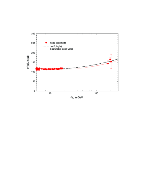
Figure 1: The dashed curve is $\sigma_{\rm tot}(\gamma p)$, the predicted total $\gamma p$ cross section from eq. (6), using the central value parameters $A=115$, $c=35.1$, $\beta=1.07$, $s_{0}=68.4$ GeV², and $\mu=0.5$ of a $\chi^{2}$ fit, compared to the existing high energy experimental data in the c.m.s. energy interval $5{\ \rm GeV}\leq\sqrt{s}\leq 200$ GeV. The dotted curve varies the parameters slightly, with $A\rightarrow 107$ and $c\rightarrow 134$ (values within their errors). The corresponding $\rho_{\gamma p}$ curves are shown in Fig. 2.

Using eq. (7), Fig. 2 shows our result for $\rho_{\gamma p}$ compared to $\rho_{nn}$, the $\rho$-value for nucleon-nucleon scattering found in ref. [4], as a function of the c.m.s. energy $\sqrt{s}$, in GeV. The solid curve is $\rho_{nn}$; the dashed line is the $\rho_{\gamma p}$ curve which corresponds to the central values $A=115$, $c=35.1$, $\beta=1.07$, $s_{0}=68.4$ GeV²; the dotted line is the $\rho_{\gamma p}$ curve which uses the slightly varied parameters $A=107$ and $c=134$.

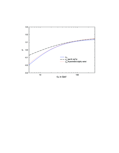
Figure 2: The solid curve is $\rho_{\rm nn}$, the predicted ratio of the real to imaginary part of the forward scattering amplitude for the ‘elastic reactions , $\gamma+p\rightarrow V+p$ scattering amplitude, where $V$ is $\rho$, $\omega$ or $\phi$ (using factorization). The dashed curve is $\rho_{\gamma p}$, the ratio of the real to imaginary part of the forward scattering amplitude for Compton scattering , $\gamma+p\rightarrow\gamma+p$, found from eq. (7), using real analytic amplitudes that asymptotically go as $\ln^{2}s$, with best fit parameters $A=115$, $c=35.1$, $\beta=1.07$, $s_{0}=68.4$ GeV², and $\mu=0.5$. The dotted line is the $\rho_{\gamma p}$ curve where the parameters of the fit have been slightly varied within their errors, with $A\rightarrow 107$ and $c\rightarrow 134$. The corresponding two curves for $\sigma_{\rm tot}(\gamma p)$ are shown in Fig. 1.

The agreement between the slightly modified $\rho_{\gamma p}$ and $\rho_{nn}$ over the energy interval $5\ {\rm GeV}\leq\sqrt{s}\leq 200$ GeV lends experimental support, in a model independent way, for the three factorization theorems of Block and Kadailov[5, 7]. Of course, precision cross section data in the region $20\ {\rm GeV}<\sqrt{s}<200$ GeV would enable us to strengthen this conclusion.

4 Acknowledgments

The author would like to thank Professor J. D. Jackson for valuable critical comments and suggestions.

References

• [1] M.Β M.Β Block and R.Β N.Β Cahn, Rev.Β Mod.Β Phys.Β 57, 563 (1985).
• [2] C.Β Bourrely and J.Β Fischer, Nucl. Phys. B 61, 513 (1973).
• [3] M.Β Damashek and F.Β Gilman, Phys. Rev. D 1, 1319 (1970).
• [4] M.Β M.Β Block et al., e-Print Archive: hep-ph/0004232, Phys. Rev. D62, 077501 (2000).
• [5] M. M. Block and A. B. Kaidalov, e-Print Archive: hep-ph/0012365, Phys. Rev. D 64, 076002 (2001).
• [6] D.Β E.Β Groom et al., Eur. Phys. J. C 15, 1 (2000).
• [7] M.Β M.Β Block et al., e-Print Archive: hep-ph/0111046 v2, Eur. Phys. J. C 23, 329 (2002).