Signals of the Abelian $Z^{\prime}$ boson within the model independent analysis of the LEP data

Abstract

The preliminary LEP data set on the total cross sections and the forward-backward asymmetries of the $e^{+}e^{-}\rightarrow\bar{f}f$ processes are analysed to establish a model-independent search for the signals of the virtual Abelian $Z^{\prime}$ boson. The recently introduced observables giving possibility to pick up uniquely the $Z^{\prime}$ signals in these processes are used. The mean values of the observables are in accordance with the $Z^{\prime}$ detection at the $1\sigma$ accuracy. The results of other model-independent fits and further prospects are discussed.

1 Introduction

The recently finished LEP2 experiments have accumulated a huge amount of data allowing to verify the predictions of the Standard Model (SM) of elementary particles as well as to estimate the energy scale of new physics beyond the SM. Although the complete set of the LEP2 data is still being combined, the preliminary total cross sections and the forward-backward asymmetries have already been adduced in the literature [1].

In the present note we are going to discuss the problem of searching for signals of the heavy Abelian $Z^{\prime}$ boson [2] by means of analysis of the LEP data on the $e^{+}e^{-}\rightarrow\bar{f}f$ processes. This particle is the necessary element of different models extending the SM. The low limits on its mass estimated for the variety of popular models ($\chi$, $\psi$, $\eta$, L–R models [3] and the Sequential Standard Model (SSM) [4]) are found to be in the energy interval 500–2000 GeV [1] (see Table 1 which reproduces Table 8.9 of Ref. [1]). As it is seen, the values of $m_{Z^{\prime}}$ (as well as the $Z^{\prime}$ couplings to the SM particles) are strongly model-dependent.

Other approach to find signals of new physics beyond the SM is the model-independent analysis. In this consideration a number of different contact interactions is introduced instead of specifying the heavy particle content. Since only one parameter of new physics can be successfully fitted, the LEP Collaborations usually discuss eight ‘models’ (LL, RR, LR, RL, VV, AA, A0, V0) which assume specific helicity couplings between the initial state and the final state fermion currents. Each model is described by only one non-zero four-fermion coupling, while others are set to zero. For example, in the LL model the non-zero coupling of left-handed fermions is taken into account. The signal of a new heavy particle is fitted by considering the interference of the SM amplitude with the contact four-fermion term. Whatever physics beyond the SM exists, it has to manifest itself in some contact coupling mentioned. Hence, it is possible to find a low limit on the masses of the states responsible for the interactions considered. In principle, a number of states may contribute into each of the models. Therefore, the purpose of the fit described by these models is to find any signal of new physics. No specific types of new particles are considered in these models. However, the virtual states of a realistic heavy particle (for instance, the Abelian $Z^{\prime}$ boson) contribute to several contact interactions simultaneously and the corresponding couplings cannot be switched off separately.

Notice the fits for the process $e^{+}e^{-}\to\mu^{+}\mu^{-}$ in Ref. [1]. A half of the eight models mentioned demonstrates the one standard deviation from the SM predictions. In this regard, we note Ref. [5] where these models were applied to the Bhabha scattering $e^{+}e^{-}\to e^{+}e^{-}(\gamma)$. The deviations from the SM at the $1\sigma$–level were found again, whereas the AA model shows the $2\sigma$–level deviation. However, these deviations could not be interpreted as the signal of the Abelian $Z^{\prime}$ boson.

Because of the mentioned arguments it seems to us reasonable to find some model independent signals of the $Z^{\prime}$ boson. To elaborate that we have taken into consideration some general principles of the field theory which give possibility to relate the parameters of different scattering processes. Then we introduced the variables, convenient to pick up uniquely the $Z^{\prime}$ boson (or other heavy states). In Ref. [6] the model-independent sign-definite observables for the Abelian $Z^{\prime}$ detection in four-fermion scattering processes at $\sqrt{s}\simeq 500$ GeV were introduced.

As it was pointed out in Ref. [6], some $Z^{\prime}$ couplings to the SM particles could be related by using the requirement of renormalizability of the underlying model remaining in other respects unspecified. The relations between the parameters of new physics appearing due to the renormalizability were called the renormalization group (RG) relations. The derived in Ref. [6] RG relations predict two possible types of the low-energy $Z^{\prime}$ interactions with the SM fields, namely, the chiral and the Abelian $Z^{\prime}$ bosons. Each $Z^{\prime}$ type is described by a few couplings to the SM fields. Therefore, it is possible to introduce observables which uniquely pick up the $Z^{\prime}$ virtual state [6]. In the present paper we discuss the observables at LEP energies and the constraints on possible signals of Abelian $Z^{\prime}$-boson following from the analysis of the LEP data. The content of the paper is the following. In sect. 2 the necessary information on the model-independent description of the $Z^{\prime}$ interactions at low energies and the RG relations are given. In sect. 3 the observables to pick up uniquely the $Z^{\prime}$ boson are introduced. In the last section the results on the LEP data fit and the conclusions as well as further prospects are discussed.

2 $Z^{\prime}$ couplings to fermion and scalar fields

The Abelian $Z^{\prime}$ boson can be introduced in a phenomenological way by defining its effective low-energy couplings to the SM fields. Such a parameterization is well known in the literature [2]. Since we are going to account of the $Z^{\prime}$ effects in the low-energy $e^{+}e^{-}\to l^{+}l^{-}$ processes, we consider the tree-level $Z^{\prime}$ interactions, only. As the decoupling theorem [7] guarantees, they are of renormalizable type, since the non-renormalizable interactions are generated at higher energies due to radiation corrections and suppressed by the inverse heavy mass. The SM gauge group $SU(2)_{L}\times U(1)_{Y}$ is considered as a subgroup of the underlying theory group. So, the mixing interactions of the types $Z^{\prime}W^{+}W^{-}$, $Z^{\prime}ZZ$, … are absent at the tree level. Under these assumptions the $Z^{\prime}$ couplings to the fermion and scalar fields are described by the Lagrangian:

$${\cal L} = \left|\left(D^{{\rm ew,}\phi}_{\mu}-\frac{i\tilde{g}}{2}\tilde{Y}(\phi)\tilde{B}_{\mu}\right)\phi\right|^{2}+$$ (1)

$$i\sum\limits_{f=f_{L},f_{R}}\bar{f}{\gamma^{\mu}}\left(D^{{\rm ew,}f}_{\mu}-\frac{i\tilde{g}}{2}\tilde{Y}(f)\tilde{B}_{\mu}\right)f,$$

where $\phi$ is the SM scalar doublet, $\tilde{B}_{\mu}$ denotes the massive $Z^{\prime}$ field before the spontaneous breaking of the electroweak symmetry, and the summation over the all SM left-handed fermion doublets, $f_{L}=\{(f_{u})_{L},(f_{d})_{L}\}$, and the right-handed singlets, $f_{R}=(f_{u})_{R},(f_{d})_{R}$, is understood. The notation $\tilde{g}$ stands for the charge corresponding to the $Z^{\prime}$ gauge group, $D^{{\rm ew,}\phi}_{\mu}$ and $D^{{\rm ew,}f}_{\mu}$ are the electroweak covariant derivatives. Diagonal $2\times 2$ matrices $\tilde{Y}(\phi)={\rm diag}(\tilde{Y}_{\phi,1},\tilde{Y}_{\phi,2})$, $\tilde{Y}(f_{L})={\rm diag}(\tilde{Y}_{L,f_{u}},\tilde{Y}_{L,f_{d}})$ and numbers $\tilde{Y}(f_{R})=\tilde{Y}_{R,f}$ are unknown $Z^{\prime}$ generators characterizing the model beyond the SM.

In particular, the Lagrangian (1) describes the $Z$–$Z^{\prime}$ mixing of order $m^{2}_{Z}/m^{2}_{Z^{\prime}}$ which is proportional to $\tilde{Y}_{\phi,2}$ and originated by the diagonalization of the neutral boson states. The mixing contributes to the scattering amplitudes and cannot be neglected at the LEP energies [8].

Thus, the $Z^{\prime}$ couplings to any fermion $f$ are parameterized by the numbers $\tilde{Y}_{L,f}$ and $\tilde{Y}_{R,f}$. Alternatively, one can use the couplings to the axial-vector and vector fermion currents, $a^{l}_{Z^{\prime}}\equiv(\tilde{Y}_{R,l}-\tilde{Y}_{L,l})/2$ and $v^{l}_{Z^{\prime}}\equiv(\tilde{Y}_{L,l}+\tilde{Y}_{R,l})/2$.

The parameters $a_{f}$, $v_{f}$ are usually treated as independent numbers. However, they are related if the underlying theory is renormalizable. The detailed discussion of this point as well as the derivation of the RG relations are given in Ref. [6]. Therein it is shown that two possible types of the $Z^{\prime}$ bosons are possible – the chiral and the Abelian ones. In the present paper we are interested in the Abelian $Z^{\prime}$ couplings which are described by the relations:

$$v_{f}-a_{f}=v_{f^{\star}}-a_{f^{\star}},\quad a_{f}=T_{3,f}\tilde{Y}_{\phi},\quad\tilde{Y}_{\phi,1}=\tilde{Y}_{\phi,2}\equiv\tilde{Y}_{\phi}$$ (2)

where $T^{3}_{f}$ is the third component of the fermion weak isospin, and $f^{\star}$ means the isopartner of $f$ (namely, $l^{\star}=\nu_{l},\nu^{\star}_{l}=l,\ldots$). The relations (2) ensure, in particular, the invariance of the Yukawa terms with respect to the effective low-energy $\tilde{U}(1)$ subgroup corresponding to the Abelian $Z^{\prime}$ boson. As it follows from the relations, the couplings of the Abelian $Z^{\prime}$ to the axial-vector fermion currents have the universal absolute value proportional to the $Z^{\prime}$ coupling to the scalar doublet. So, in what follows we will use the short notation $a=a_{l}=-\tilde{Y}_{\phi}/2$.

Notice that the same relations (2) hold in the two-Higgs-doublet model (THDM) [9]. As a consequence, the results of the present note are also valid for the case of the THDM as the low-energy theory.

Because of a fewer number of independent $Z^{\prime}$ couplings it is possible to introduce the observables convenient for detecting uniquely the $Z^{\prime}$ signals in experiments. In what follows, we take into account the RG relations (2) in order to constrain signals of the Abelian $Z^{\prime}$ boson.

3 Observables

Consider the lepton processes $e^{+}e^{-}\to V^{\ast}\to l^{+}l^{-}$ ($l=\mu,\tau$) with the neutral vector boson exchange ($V=A,Z,Z^{\prime}$). We assume the non-polarized initial- and final-state fermions. At LEP energies $\sqrt{s}\simeq 200$ GeV the leptons can be treated as massless particles. In this approximation the left-handed and the right-handed fermions can be substituted by the helicity states.

To take into consideration the correlations (2) let us introduce the observable $\sigma_{l}(z)$ defined as the difference of cross sections integrated in some ranges of the scattering angle $\theta$:

$$\sigma_{l}(z) \equiv \int\nolimits_{z}^{1}\frac{d\sigma_{l}}{d\cos\theta}d\cos\theta-\int\nolimits_{-1}^{z}\frac{d\sigma_{l}}{d\cos\theta}d\cos\theta$$

$$= \sigma^{T}_{l}\left[A^{FB}_{l}\left(1-z^{2}\right)-\frac{z}{4}\left(3+z^{2}\right)\right],$$

$$\Delta\sigma_{l}(z) \equiv \sigma_{l}(z)-\sigma^{\rm SM}_{l}(z),$$ (3)

where $z$ stands for the cosine of the boundary angle, $\sigma^{T}_{l}$ denotes the total cross section and $A^{FB}_{l}$ is the forward-backward asymmetry of the process. The idea of introducing the $z$-dependent observable (3) is to choose the value of the kinematic parameter $z$ in such a way that to pick up the characteristic features of the Abelian $Z^{\prime}$ signals. Since the observable $\Delta\sigma_{l}(z)$ is a small quantity, it can be computed in lower order by the Born amplitudes for $e^{+}e^{-}\to V^{\ast}\to l^{+}l^{-}$ $(V=\gamma,Z,Z^{\prime})$.

The expansion of the $Z^{\prime}$-boson propagator $(s-m^{2}_{Z^{\prime}})^{-1}$ and the $Z$–$Z^{\prime}$ mixing angle in the inverse $Z^{\prime}$ mass produces a number of terms of order $m^{-2}_{Z^{\prime}}$ and higher. The lower-level contributions describe the four-fermion contact interactions and contain the ratio $\tilde{g}^{2}/m^{2}_{Z^{\prime}}$ of the $Z^{\prime}$ mass and the charge $\tilde{g}$, only. Thus, the quantities $m_{Z^{\prime}}$ and $\tilde{g}$ cannot be measured separately by the fit of observables in the leading order in $m^{-2}_{Z^{\prime}}$. In what follows we will also treat the terms of order $m^{-4}_{Z^{\prime}}$. As we will show, these contributions allow one to fit both the four-fermion coupling constant $\tilde{g}^{2}/m^{2}_{Z^{\prime}}$ and the $Z^{\prime}$ mass, if the cross sections at different center-of-mass energies are taken into account.

Due to the correlations between the Abelian $Z^{\prime}$ couplings the cross section (3) can be written as follows

$$\Delta\sigma_{l}(z)=\sum_{j=0}^{2}\left[A_{j}(s,z)+\zeta B_{j}(s,z)\right]\epsilon_{j}+\sum_{j=0}^{2}\sum_{k=0}^{j}C_{jk}(s,z)\epsilon_{j}\epsilon_{k},$$ (4)

where we introduce the dimensionless quantities

$$\epsilon_{0} = \frac{\tilde{g}^{2}m^{2}_{Z}a^{2}}{4\pi m^{2}_{Z^{\prime}}},\quad\epsilon_{1}=\frac{\tilde{g}^{2}m^{2}_{Z}v_{e}v_{l}}{4\pi m^{2}_{Z^{\prime}}},$$

$$\epsilon_{2} = \frac{\tilde{g}^{2}m^{2}_{Z}a(v_{e}+v_{l})}{4\pi m^{2}_{Z^{\prime}}},\quad\zeta=\frac{m^{2}_{Z}}{m^{2}_{Z^{\prime}}}.$$ (5)

The functions $A_{j}(z,s)$, $B_{j}(z,s)$ and $C_{jk}(z,s)$ are determined by the SM couplings and masses, only. They are also independent of the lepton generation. The factors $A_{j}$ describe the leading-order contributions, whereas others correspond to the higher-order corrections in the inverse $Z^{\prime}$ mass.

As it was argued in Refs. [8, 10], there is a region of values $z$, at which all the factors $A_{j}$ except for $A_{0}$ contribute less than 2%. Since the parameter $\epsilon_{0}$ is a positive quantity by the definition, it is possible to construct a sign-definite observable by specifying the appropriate value of the kinematic parameter $z$. This value, $z=z^{*}$, can be chosen in order to maximize the relative contribution of the sign-definite terms in $\Delta\sigma_{l}(z)$. To take into account the order of each term in the inverse $Z^{\prime}$ mass, we introduce positive ‘weights’ $\omega_{B}\sim\zeta$ and $\omega_{C}\sim|\epsilon_{j}|$ for the higher-order contributions. Thus, $z^{*}$ is found by the maximization of the following function:

$$F=\frac{|A_{0}|+\omega_{B}|B_{0}|+\omega_{C}|C_{00}|}{\sum_{j=0}^{2}\left(|A_{j}|+\omega_{B}|B_{j}|+\sum_{k=0}^{j}\omega_{C}|C_{jk}|\right)}.$$ (6)

The numeric values of the ‘weights’ $\omega_{B}$ and $\omega_{C}$ can be taken from the present day bounds on the contact couplings [1] or [11]. As the computation shows, the value of $z^{*}$ with the accuracy $10^{-3}$ depends on the order of the ‘weight’ magnitudes, only. So, in what follows we take $\omega_{B}\sim.004$ and $\omega_{C}\sim 0.00004$.

The function $z^{\ast}(s)$ is the decreasing function of the center-of-mass energy. It is tabulated for the LEP energies in Table 2. The corresponding values of the maximized function $F$ are within the interval $0.960<F<0.966$.

Since $A_{0}(s,z^{*})<0$, $B_{0}(s,z^{*})<0$ and $C_{00}(s,z^{*})<0$, the observable

$$\Delta\sigma_{l}(z^{*})=\left[A_{0}(s,z^{*})+\zeta B_{0}(s,z^{*})\right]\epsilon_{0}+C_{00}(s,z^{*})\epsilon^{2}_{0}$$ (7)

is negative and the same for the all types of the SM charged leptons with the accuracy 2–4%. This observable selects the model-independent signal of the Abelian $Z^{\prime}$ boson in the processes $e^{+}e^{-}\to l^{+}l^{-}$.

4 Data fit and Conclusions

To search for the model-independent $Z^{\prime}$ signals we will analyze the introduced observable $\Delta\sigma_{l}(z^{\ast})$ on the base of the LEP data set. In the lower order in $m^{-2}_{Z^{\prime}}$ the observable (7) depends on the one parameter, $\epsilon_{0}$,

$$\Delta\sigma^{\rm th}_{l}(z^{*})=A_{0}(s,z^{*})\epsilon_{0}+C_{00}(s,z^{*})\epsilon^{2}_{0},$$ (8)

which can be fitted from the experimental values of $\Delta\sigma_{l}(z^{\ast})$. This approach has the following advantages:

1. All the LEP data for the lepton processes $e^{+}e^{-}\to l^{+}l^{-}$ can be incorporated to obtain the limits on the same flavour-independent scale.

2. The sign of the fitted parameter ($\epsilon_{0}>0$) is the characteristic feature of the Abelian $Z^{\prime}$ signal.

The LEP data for the total cross-sections and the forward-backward asymmetries [1] are converted to the experimental values of the observable $\Delta\sigma_{l}(z^{\ast})$ with the corresponding errors $\delta\sigma_{l}(z^{\ast})$ for each LEP energy by means of the following relations:

$$\Delta\sigma_{l}(z^{\ast}) = \left[A_{l}^{FB}\left(1-z^{\ast 2}\right)-\frac{z^{\ast}}{4}\left(3+z^{\ast 2}\right)\right]\Delta\sigma_{l}^{T}$$

$$+\left(1-z^{\ast 2}\right)\sigma_{l,\rm SM}^{T}\Delta A_{l}^{FB},$$

$$\delta\sigma_{l}(z^{\ast})^{2} = {\left[A_{l}^{FB}\left(1-z^{\ast 2}\right)-\frac{z^{\ast}}{4}\left(3+z^{\ast 2}\right)\right]}^{2}(\delta\sigma_{l}^{T})^{2}$$ (9)

$$+{\left[\left(1-z^{\ast 2}\right)\sigma_{l,\rm SM}^{T}\right]}^{2}(\delta A_{l}^{FB})^{2}.$$

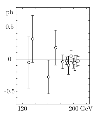
Figure 1: $\Delta\sigma_{\mu}(z^{\ast})$ computed from the LEP data.

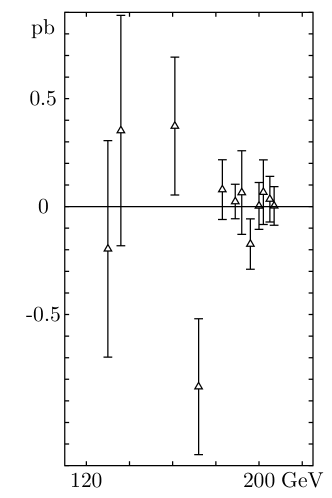
Figure 2: $\Delta\sigma_{\tau}(z^{\ast})$ computed from the LEP data.

The results are given in Table 2 and Figs. 1–2.

As it is seen, all the values of the observable are no more than one standard deviation from the SM value $\Delta\sigma_{l}(z^{*})=0$ except for the value of $\Delta\sigma_{\mu}$ at 161 GeV and three points at 161, 172 and 196 GeV corresponding to the $e^{+}e^{-}\to\tau^{+}\tau^{-}$ process. These points reflect the significant dispersion of the measurements at $\sqrt{s}<183$ GeV. As it is also seen from Figs. 1–2, the measurements for the scattering into $\mu$ pairs have a higher level of precision. Thus, in what follows we will use two sets of data: 12 points for the $e^{+}e^{-}\to\mu^{+}\mu^{-}$ process and the full data set including 24 points for $\mu^{+}\mu^{-}$ and $\tau^{+}\tau^{-}$ in the final state.

The central value of the fitted parameter $\epsilon_{0}$ is obtained as the result of minimization of the $\chi^{2}$-function:

$$\chi^{2}(\epsilon_{0})=\sum_{n}\frac{\left[\Delta\sigma^{\rm ex}_{l,n}(z^{*})-\Delta\sigma^{\rm th}_{l}(z^{*})\right]^{2}}{\delta\sigma^{\rm ex}_{l,n}(z^{*})^{2}},$$ (10)

where the sum runs over the experimental points entering the data set chosen.

The $1\sigma$ confidence level interval $(b_{1},b_{2})$ for the fitted parameter is derived by means of the likelihood function ${\cal L}(\epsilon_{0})\propto\exp[-\chi^{2}(\epsilon_{0})/2]$. It is determined by the equations:

$$\int\nolimits_{b_{1}}^{b_{2}}{\cal L}(\epsilon^{\prime})d\epsilon^{\prime}=0.68,\quad{\cal L}(b_{1})={\cal L}(b_{2}).$$ (11)

To compare our results with those of Ref. [1] we introduce the contact interaction scale

$$\Lambda^{2}=4m^{2}_{Z}\epsilon^{-1}_{0}.$$ (12)

This normalization of contact couplings is admitted in Ref. [1]. We use the log-likelihood method to determine a one sided lower limit on the scale $\Lambda$ at the 95% confidence level. It is derived by the integration of the likelihood function over the physically allowed region $\epsilon_{0}>0$. The exact definition is

$$\Lambda=2m_{Z}(\epsilon^{*})^{-1/2},\quad\int_{0}^{\epsilon^{*}}{\cal L}(\epsilon^{\prime})d\epsilon^{\prime}=0.95\int_{0}^{\infty}{\cal L}(\epsilon^{\prime})d\epsilon^{\prime}.$$ (13)

We also introduce the probability of the Abelian $Z^{\prime}$ signal as the integral of the likelihood function over the positive values of $\epsilon_{0}$:

$$P=\int\nolimits_{0}^{\infty}L(\epsilon^{\prime})d\epsilon^{\prime}.$$ (14)

As it was mentioned above, we choose two different sets of data to fit the parameter $\epsilon_{0}$. The first one includes $e^{-}e^{+}\to\mu^{-}\mu^{+}$ scattering data (12 points), whereas the second set includes both $e^{-}e^{+}\to\mu^{-}\mu^{+}$ and $e^{-}e^{+}\to\tau^{-}\tau^{+}$ data (24 measurements). In Table 3 we show the fitted values of $\epsilon_{0}$ with their 68% confidence level uncertainties, the 95% confidence level lower limit on the scale $\Lambda$, and the total probability of the Abelian $Z^{\prime}$ signal.

As it is seen, all the data sets lead to the comparable fitted values of $\epsilon_{0}$ with the nearly equal uncertainties. All the central values, $\bar{\epsilon}_{0}$, have the sign compatible with the Abelian $Z^{\prime}$ signal. The more precise data corresponding to the scattering into $\mu^{+}\mu^{-}$ pairs demonstrate the largest positive mean value of $\epsilon_{0}$. This value is at one standard deviation from the SM prediction $\bar{\epsilon}_{0}=0$.

Taking into account the data for $\tau^{+}\tau^{-}$ final states decreases the central value of $\epsilon_{0}$ but does not affect essentially the uncertainty of the result. The corresponding fitted value is no more than one standard deviation.

Thus, the fitted central values $\bar{\epsilon}_{0}$ witness to the Abelian $Z^{\prime}$ existence. The signal is at one standard deviation for the $e^{-}e^{+}\to\mu^{-}\mu^{+}$ data. No signal is found at the $1\sigma$ confidence level for the full lepton data set.

In fact, the fitted value of the contact coupling $\epsilon_{0}$ originates from the leading-order term in the inverse $Z^{\prime}$ mass contributing to the observable (7). The analysis of the higher-order terms allows to estimate the constraints on the $Z^{\prime}$ mass alone. Substituting $\epsilon_{0}$ in Eq. (7) by its fitted central value from Table 3, $\bar{\epsilon}_{0}$, one obtains the expression

$$\Delta\sigma_{l}(z^{*})=\left[A_{0}(s,z^{*})+\zeta B_{0}(s,z^{*})\right]\bar{\epsilon}_{0}+C_{00}(s,z^{*})\bar{\epsilon}^{2}_{0},$$ (15)

which depends on the parameter $\zeta=m^{2}_{Z}/m^{2}_{Z^{\prime}}$.

The central value of $\zeta$ and the $1\sigma$ confidence interval can be computed in a way as those for $\epsilon_{0}$. The results are also given in Table 3.

Being governed by the next-to-leading contributions in $m^{-2}_{Z^{\prime}}$, the fitted values of $\zeta$ are characterized by significant errors. The $\mu\mu$ data set gives the central value which corresponds to $m_{Z^{\prime}}\simeq 1.13$ TeV, whereas the full lepton data set leads to the unphysical central value of $\zeta$. Of course, the derived constraints on $\zeta$ are rather an illustration of the possibility to fit the $Z^{\prime}$ mass alone because the higher-order terms in $m^{-2}_{Z^{\prime}}$ have to be accounted for simultaneously with the loop corrections to the factors $A_{0}$, $B_{0}$ and $C_{00}$ in Eq. (7). So, the analysis of the terms $\sim m^{-4}_{Z^{\prime}}$ requires to compute $\Delta\sigma_{l}(z^{*})$ in the improved Born approximation, which is the subject for separate investigations. The important possibility to improve accuracy is to use the data on the differential cross sections, when the combined data on them will be completed. With these data taken into consideration the observable $\Delta\sigma_{l}(z^{*})$ can be calculated directly from the definition Eq. (3). In this case the uncertainties have to decrease. We believe that all these stages of the improvement of the data treating will make the situation with the $Z^{\prime}$ signals more transparent.

As it was shown, the characteristic signal of the Abelian $Z^{\prime}$ boson is concerned with the coupling to axial-vector currents. In this regard, let us turn again to the helicity ‘models’ of Ref. [1] and compare our results with the fit for the AA case. As it follows from the present analysis, this model is sensitive mainly to the signals of the Abelian $Z^{\prime}$ boson. Of course, the parameters $\epsilon$ in Ref. [1] and $\epsilon_{0}$ in Eq. (3) are not the same quantity. First, they are normalized by different factors and related as $\epsilon=-\epsilon_{0}m^{-2}_{Z}/4$. Second, as we already noted, in the AA model the $Z^{\prime}$ couplings to the vector fermion currents are set to zero, therefore it is able to describe only some particular case of the Abelian $Z^{\prime}$ boson. Moreover, in this model both the positive and the negative values of $\epsilon$ are considered, whereas in our approach only the positive $\epsilon_{0}$ values (which correspond to the negative $\epsilon$) are permissible. As the value of the four-fermion contact coupling in the AA model is dependent on the lepton flavor, the Abelian $Z^{\prime}$ induces the axial-vector coupling which is universal for all lepton types. Nevertheless, it is interesting to note that the fitted value of $\epsilon$ in the AA model for the $\mu^{+}\mu^{-}$ final states ($-0.0025^{+0.0018}_{-0.0023}\mbox{ TeV}^{-2}$) as well as the value derived under the assumption of the lepton universality ($-0.0018^{+0.0016}_{-0.0019}\mbox{ TeV}^{-2}$) are similar to our results which correspond to $\epsilon=-0.0014^{+0.0014}_{-0.0014}\mbox{ TeV}^{-2}$ and $\epsilon=-0.0009^{+0.0011}_{-0.0011}\mbox{ TeV}^{-2}$, respectively. Thus, the signs of the central values in the AA model agree with our results, whereas the uncertainties are of the same order. From the carried out analysis it follows that the AA model is mainly responsible for signals of the Abelian $Z^{\prime}$ gauge boson although a lot of details concerning its interactions is not accounted for within this fit.

The $Z^{\prime}$ boson mass is related to the contact interaction scale $\epsilon_{0}$ by Eq. (3). If the $Z^{\prime}$ boson couples to the SM particles with a strength comparable with the electroweak forces $\tilde{g}\simeq g$, the central values of $\bar{\epsilon}_{0}$ correspond to the masses of order 3–4 TeV, whereas the lower limit on $m_{Z^{\prime}}$ is about 1.5–1.7 TeV. Thus, although the $Z^{\prime}$ boson is not detected at LEP, it could be light enough to be discovered at LHC.

5 Acknowledgement

A.G. thanks D.Kazakov, S.Mikhailov and O.Teryaev for fruitful discussions and the JINR for its hospitality while this work was being completed.

Table 1: 95% confidence level lower limits on the $Z^{\prime}$ mass for some popular models.

Model	$\chi$	$\psi$	$\eta$	L–R	SSM
$m^{\rm limit}_{Z^{\prime}},{\rm GeV}/c^{2}$	678	463	436	800	1890

Table 2: The boundary angle $z^{\ast}$ and the observable $\Delta\sigma_{l}(z^{\ast})$ (pb) computed at energies of the LEP experiments.

$\sqrt{s}$, GeV	$z^{*}$	$\Delta\sigma_{\mu}(z)$, pb	$\Delta\sigma_{\tau}(z)$, pb
130	0.486	$-0.053\pm 0.398$	$-0.196\pm 0.501$
136	0.464	$0.313\pm 0.364$	$0.352\pm 0.534$
161	0.406	$-0.278\pm 0.262$	$0.373\pm 0.319$
172	0.391	$0.178\pm 0.271$	$-0.834\pm 0.315$
183	0.379	$-0.042\pm 0.107$	$0.079\pm 0.138$
189	0.374	$-0.026\pm 0.060$	$0.023\pm 0.080$
192	0.372	$-0.096\pm 0.142$	$0.065\pm 0.194$
196	0.369	$0.047\pm 0.082$	$-0.174\pm 0.117$
200	0.366	$-0.065\pm 0.078$	$0.003\pm 0.109$
202	0.364	$-0.059\pm 0.118$	$0.067\pm 0.150$
205	0.362	$-0.034\pm 0.086$	$0.034\pm 0.106$
207	0.361	$-0.029\pm 0.068$	$0.003\pm 0.089$

Table 3: The fitted values of the contact coupling $\epsilon_{0}$ and their 68% confidence level uncertainties, the 95% confidence level lower limit on the scale $\Lambda$, the probability of the $Z^{\prime}$ signal, $P$, and the fitted values of $\zeta=m^{2}_{Z}/m^{2}_{Z^{\prime}}$ from the analysis of terms $\sim m^{-4}_{Z^{\prime}}$.

Data set	$\epsilon_{0}$	$\Lambda$, TeV	$P$	$\zeta$
$\mu\mu$	$0.0000455^{+0.0000459}_{-0.0000462}$	16.3	0.83	$0.006\pm 0.213$
$\mu\mu$ and $\tau\tau$	$0.000030\pm 0.000037$	18.7	0.79	$-0.029\pm 0.231$

References

• [1] ALEPH Collaboration, DELPHI Collaboration, L3 Collaboration, OPAL Collaboration, the LEP Electroweak Working Group, the SLD Heavy Flavour, Electroweak Working Group, hep-ex/0112021.
• [2] A. Leike, Phys. Rep. 317, 143 (1999).
• [3] P. Langacker, R.W. Robinett, and J.L. Rosner, Phys. Rev. D 30, 1470 (1984); D. London and J.L. Rosner, Phys. Rev. D 34, 1530 (1986); J.C. Pati and A. Salam, Phys. Rev. D 10, 275 (1974); R.N. Mohapatra and J.C. Pati, Phys. Rev. D 11, 566 (1975).
• [4] G. Altarelli et al., Z. Phys. C 45, 109 (1989).
• [5] D. Bourilkov, Phys. Rev. D 64, 071701 (2001).
• [6] A. Gulov and V. Skalozub, Eur. Phys. J. C 17, 685 (2000).
• [7] T. Appelquist and J. Carazzone, Phys. Rev. D 11, 2856 (1975).
• [8] A. Gulov and V. Skalozub, Nucl. Phys. Proc. Suppl. 102, 363 (2001).
• [9] J. Gunion, H. Haber, G. Kane, and S. Dawson, The Higgs Hunter’s Guide, Addison-Wesley, Reading, MA, 1990; R. Santos and A. Barroso, Phys. Rev. D 56, 5366 (1997).
• [10] A. Gulov and V. Skalozub, Phys. Rev. D 61, 055007 (2000).
• [11] A. Gulov and V. Skalozub, hep-ph/0107236.