-1cm 0cm 0cm 23cm 0.2cm 16cm IPPP/02/21 DTP/02/42 REVISED June 2002

Abstract

We consider the behaviour of the perturbative QCD corrections to the $R_{{e^{+}}{e^{-}}}$ ratio, in the limit that the c.m. energy $\sqrt{s}$ vanishes. Writing $R_{{e^{+}}{e^{-}}}(s)=3{\sum_{f}}{Q}_{f}^{2}(1+{\cal{R}}(s))$, with $Q_{f}$ denoting the electric charge of quark flavour $f$, we find that for ${N_{f}}<9$ flavours of massless quarks, the perturbative correction ${\cal{R}}(s)$ to the parton model result smoothly approaches from below the infra-red limit ${\cal{R}}(0)=2/b$, as $s{\rightarrow}0$. Here $b=(33-2{N_{f}})/6$ is the first QCD beta-function coefficient. This freezing holds to all-orders in perturbation theory. The $s$-dependence can be written analytically in closed form in terms of the Lambert $W$ function.

In the ultra-violet ${s}{\rightarrow}{\infty}$ limit of QCD the renormalized coupling vanishes, and this property of Asymptotic Freedom underwrites the successful use of perturbative methods in testing the theory [1]. In the infra-red limit $s{\rightarrow}0$, however, one may expect that perturbation theory will break down , with typically a Landau pole singularity in the coupling when $s{\sim}{\Lambda}_{QCD}^{2}$, and that non-perturbative effects will be important. However, the phenomenological virtues of assuming a frozen couplant, with the renormalized ${\alpha}_{s}(s)$ approaching a constant value ${\alpha}_{s}(0)/{\pi}\sim{0.3}$ in the infra-red have long been recognised [2-5]. In a pioneering paper Mattingly and Stevenson investigated the behaviour of the perturbative corrections to ${R}_{{e^{+}}{e^{-}}}$ including third-order QCD corrections, in the framework of the Principle of Minimal Sensitivity (PMS) approach [2]. Their PMS optimized coupling indeed froze to a value around $0.26$ below $300$ MeV. These predictions were then smeared using the technique of Poggio-Quinn-Weinberg (PQW) [5], and were in suprisingly good agreement with similarly smeared experimental data for ${R}_{{e^{+}}{e^{-}}}$. Some scepticism about the existence of infra-red fixed point behaviour had previously been expressed [6]. In this letter we wish to demonstrate that including all-orders in perturbation theory the perturbative corrections to ${R}_{{e^{+}}{e^{-}}}$ do freeze in the infra-red. The limiting value being $2/b$, where $b=(33-2{N_{f}})/6$ is the first beta-function coefficient of QCD with $N_{f}$ quark flavours. We assumed massless quarks and for freezing to this limit one requires ${N_{f}}<9$ flavours. In fact the freezing behaviour does not correspond to an infra-red fixed point in the beta-function, but rather stems from the energy dependence induced by analytical continuation from the Euclidean to Minkowskian region in defining ${R}_{{e}^{+}{e}^{-}}$.

We begin by defining the ${R}_{{e^{+}}{e^{-}}}$ ratio at c.m. energy $\sqrt{s}$,

$${R}_{{e^{+}}{e^{-}}}(s){\equiv}\frac{{\sigma}_{tot}({e}^{+}{e}^{-}\rightarrow\rm{hadrons})}{{\sigma}({e}^{+}{e}^{-}\rightarrow{\mu}^{+}{\mu}^{-})}=3{\sum_{f}}{Q}_{f}^{2}(1+{\cal{R}}(s))\;.$$ (1)

Here the $Q_{f}$ denote the electric charges of the different flavours of quarks, and ${\cal{R}}(s)$ denotes the perturbative corrections to the parton model result, and has a perturbation series of the form,

$${\cal{R}}(s)=a+{\sum_{n>0}}{r}_{n}{a}^{n+1}\;.$$ (2)

Here $a{\equiv}{\alpha}_{s}({\mu}^{2})/{\pi}$ is the renormalized coupling, and the coefficients $r_{1}$ and $r_{2}$ have been computed in the $\overline{MS}$ scheme with renormalization scale ${\mu}^{2}=s$ [7, 8]. ${R}_{{e}^{+}{e}^{-}}$ is directly related to the transverse part of the correlator of two vector currents in the Euclidean region,

$$({q}_{\mu}{q}_{\nu}-{g}_{{\mu}{\nu}}{q}^{2}){\Pi}(s)=4{\pi}^{2}i{\int}{d}^{4}x{e}^{iq.x}<0|T[{j}_{\mu}(x){j}_{\nu}(0)]|0>\;,$$ (3)

where $s=-{q}^{2}>0$. To avoid an unspecified constant it is convenient to take a logarithmic derivative with respect to $s$ and define the Adler $D$-function,

$${D}(s)=-s\frac{d}{ds}{\Pi}(s)\;.$$ (4)

This can be represented by Eq.(1) with the perturbative corrections ${\cal{R}}(s)$ replaced by

$${\cal{D}}(s)=a+{\sum_{n>0}}{d}_{n}{a}^{n+1}\;.$$ (5)

The Minkowskian observable ${\cal{R}}(s)$ is related to ${\cal{D}}(-s)$ by analytical continuation from Euclidean to Minkowskian. This can be elegantly formulated as an integration around a circular contour in the complex energy-squared $s$-plane [9, 10],

$${\cal{R}}(s)=\frac{1}{2{\pi}}{\int_{-{\pi}}^{\pi}}{d{\theta}}{\cal{D}}(s{e}^{i{\theta}})\;.$$ (6)

Expanding ${\cal{D}}(s{e}^{i{\theta}})$ as a power series in $\bar{a}{\equiv}{a}(s{e}^{i{\theta}})$, and performing the ${\theta}$ integration term-by-term, leads to a “contour-improved” perturbation series, in which at each order an infinite subset of analytical continuation terms present in the conventional perturbation series of Eq.(2) are resummed. It is this complete analytical continuation that builds our claimed freezing of ${\cal{R}}(s)$. In contrast Ref.[2] used the conventional fixed-order perturbative expansion of Eq.(2) in the PMS approach. It is useful to begin by considering the “contour-improved” series for the simplified case of a one-loop coupling. The one-loop coupling will be given by

$$a(s)=\frac{2}{b{\ln}(s/{\tilde{\Lambda}}_{\overline{MS}}^{2})}\;.$$ (7)

As described above one can then obtain the “contour-improved” perturbation series for ${\cal{R}}(s)$,

$${\cal{R}}(s)={A}_{1}(s)+{\sum_{n=1}^{\infty}}{d}_{n}{A}_{n+1}(s)\;,$$ (8)

where the functions ${A}_{n}(s)$ are defined by,

$${A}_{n}(s) {\equiv} \frac{1}{2{\pi}}{\int_{-{\pi}}^{\pi}}{d{\theta}}{\bar{a}}^{n}=\frac{1}{2{\pi}}{\int_{-\pi}^{\pi}}{d{\theta}}\frac{{a}^{n}(s)}{{[1+ib{\theta}a(s)/2]}^{n}}\;.$$ (9)

This is an elementary integral which can be evaluated in closed-form as [11]

$${A}_{1}(s) = \frac{2}{{\pi}b}{\arctan}\left(\frac{{\pi}ba(s)}{2}\right)$$

$${A}_{n}(s) = \frac{2{a}^{n-1}(s)}{b{\pi}(1-n)}Im\left[{\left(1+\frac{ib{\pi}a(s)}{2}\right)}^{1-n}\right]\;(n>1)\;.$$ (10)

We then obtain the one-loop “contour-improved” series for ${\cal{R}}(s)$,

$${\cal{R}}(s)=\frac{2}{\pi{b}}{\arctan}\left(\frac{\pi{b}{a}(s)}{2}\right)+{d}_{1}\left[\frac{{a}^{2}(s)}{(1+{b}^{2}{\pi}^{2}{a}^{2}(s)/4)}\right]+{d}_{2}\left[\frac{{a}^{3}(s)}{{(1+{b}^{2}{\pi}^{2}{a}^{2}(s)/4)}^{2}}\right]+\ldots\;.$$ (11)

The first $\arctan$ term is well-known, and corresponds to resumming the infinite subset of analytical continuation terms in the standard perturbation series of Eq.(2) which are independent of the $d_{n}$ coefficients. Subsequent terms corrrespond to resumming to all-orders the infinite subset of terms in Eq.(2) proportional to ${d}_{1},{d}_{2},{\ldots}$, etc. It is crucial to notice that in each case the resummation is convergent, provided that $|a(s)|<2/{\pi}{b}$. Thus, even though the series in Eqs.(2,5) are divergent because of the $n!$ growth of the $d_{n}$ coefficients, the resummations implicit in performing the integration of Eq.(6) term-by-term are well-defined. In the ultra-violet $s\rightarrow{\infty}$ limit the ${A}_{n}(s)$ vanish as required by asymptotic freedom. In the infra-red $s\rightarrow{0}$ limit, the one-loop coupling $a(s)$ has a “Landau” singularity at $s={\tilde{\Lambda}}_{\overline{MS}}^{2}$. However, the functions ${A}_{n}(s)$ resulting from resummation, if analytically continued, are well-defined for all real values of $s$. ${A}_{1}(s)$ smoothly approaches from below the asymptotic infra-red value $2/b$, whilst for $n>1$ the ${A}_{n}(s)$ vanish. Thus, as claimed, ${\cal{R}}(s)$ is asymptotic to $2/b$ to all-orders in perturbation theory. It might be thought that the existence of such an infra-red limit, independent of the higher-order structure of perturbation theory, is remarkable. In fact, however, it is to be expected. A useful analogy is the exponentiation to all-orders of large infra-red logarithms which appear for jet observables such as thrust distributions in ${e}^{+}{e}^{-}$ annihilation [1]. Here the standard fixed-order perturbation theory breaks down in the two-jet region as these logarithms become infinite. However, if the large logarithms are resummed to all-orders one builds an exponential factor , and the thrust distribution smoothly approaches zero in the two-jet region, to all-orders in perturbation theory. We should note a subtlety in our derivation above. As defined by the integration in $\theta$ around the circle in Eq.(9) the ${A}_{n}(s)$ are not defined for $s\leq{\tilde{\Lambda}}_{\overline{MS}}^{2}$ . However the ${A}_{n}(s)$ given by Eq.(10) are defined for all real $s$. A more careful derivation would use instead of the contour integral as a starting point, the dispersion relation,

$${\cal{R}}(s)=\frac{1}{2\pi{i}}{\int_{-s-i{\epsilon}}^{-s+i{\epsilon}}}{dt}\frac{{\cal{D}}(t)}{t}\;,$$ (12)

which clearly avoids the “Landau” singularity and is well-defined for all real $s$. One can directly obtain the result of Eq.(10) from the dispersion relation by simple manipulations. It should be noted that this route is equivalent to the Analytic Perturbation Theory (APT) approach, in which it is advocated that Minkowskian observables are expanded in a basis of functions ${\mathfrak{A}}_{n}(s)$ obtained by performing an integral transform of the Euclidean coupling using the dispersion relation of Eq.(12). In the case of the ${R}_{{e}^{+}{e}^{-}}$ ratio the resulting APT expansion corresponds to the “contour-improved” expansion of Eq.(8) and ${\mathfrak{A}}_{n}(s)={A}_{n}(s)$, given by Eq.(10). The infra-red freezing and absence of a “Landau pole” in the ${\mathfrak{A}}_{n}(s)$ has previously been discussed in the APT approach, and provides one of its major motivations. Analytic expressions for the one-loop ${\mathfrak{A}}_{n}(s)$ have been given, and freezing to all-loops in APT can be demonstrated. For a recent review see Ref.[12], and references therein.

We now move to the more challenging problem of what happens for realistic QCD beyond the simple one-loop approximation. The freezing is most easily analysed using a renormalization scheme in which the beta-function equation has its two-loop form,

$$\frac{\partial{a}({\mu}^{2})}{\partial{\ln}{\mu}^{2}}=-\frac{b}{2}{a}^{2}({\mu}^{2})(1+c{a}({\mu}^{2}))\;.$$ (13)

This corresponds to a so-called ’t Hooft scheme [13] in which the non-universal beta-function coefficients are all zero. Here $c=(153-19{N_{f}})/12b$ is the second universal beta-function coefficient. The key feature of these schemes is that the coupling can be expressed analytically in closed-form in terms of the Lambert $W$ function , defined implicitly by $W(z){\exp}(W(z))=z$ [14]. One has

$${a}({\mu}^{2}) = -\frac{1}{c[1+{W}_{-1}(z(\mu))]}$$

$$z(\mu) {\equiv} -\frac{1}{e}{\left(\frac{\mu}{{\tilde{\Lambda}}_{\overline{MS}}}\right)}^{-b/c}\;,$$ (14)

where ${\tilde{\Lambda}}_{\overline{MS}}$ is defined according to the convention of [15] , and is related to the standard definition [16] by ${\tilde{\Lambda}}_{\overline{MS}}={(2c/b)}^{-c/b}{\Lambda}_{\overline{MS}}$. The “$-1$” subscript on $W$ denotes the branch of the Lambert $W$ function required for Asymptotic Freedom, the nomenclature being that of Ref.[17]. Assuming a choice of renormalization scale ${\mu}^{2}=xs$ , where $x$ is a dimensionless constant, for the perturbation series of ${\cal{D}}(s)$ in Eq.(5), one can then expand the integrand in Eq.(6) for ${\cal{R}}(s)$ in powers of ${\bar{a}}\equiv{a}(xs{e}^{i{\theta}})$ , which can be expressed in terms of the Lambert $W$ function using Eq.(14),

$${\bar{a}}=\frac{-1}{c[1+W(A(s){e}^{iK{\theta}})]}$$ (15)

where

$$A(s)=\frac{-1}{e}{\left(\frac{\sqrt{xs}}{{\tilde{\Lambda}}_{\overline{MS}}}\right)}^{-{b/c}}\;\;\;,{K}=\frac{-b}{2c}\;.$$ (16)

The functions ${A}_{n}(s)$ in the “contour-improved” series are then given, using Eqs(15,16), by

$${A}_{n}(s) {\equiv} \frac{1}{2{\pi}}{\int_{-{\pi}}^{\pi}}{d{\theta}}{\bar{a}}^{n}=\frac{1}{2{\pi}}{\int_{-\pi}^{0}}{d{\theta}}\frac{{(-1)}^{n}}{c^{n}}{[1+{W}_{1}(A(s){e}^{iK{\theta}})]}^{-n}$$ (17)

$$+ \frac{1}{2\pi}{\int_{0}^{\pi}}{d{\theta}}\frac{{(-1)}^{n}}{c^{n}}{[1+{W}_{-1}(A(s){e}^{iK{\theta}})]}^{-n}\;.$$

Here the appropriate branches of the $W$ function are used in the two regions of integration. As discussed in Refs.[18, 19], by making the change of variable $w=W(A(s){e}^{iK{\theta}})$ we can then obtain

$${A}_{n}(s)=\frac{{(-1)}^{n}}{2iK{c^{n}}{\pi}}{\int^{{W}_{-1}(A(s){e}^{iK\pi})}_{{W}_{1}(A(s){e}^{-iK\pi})}}\frac{dw}{w{(1+w)}^{n-1}}\;.$$ (18)

This is an elementary integral and noting that ${W}_{1}(A(s){e}^{-iK\pi})={[{W}_{-1}(A(s){e}^{iK\pi})]}^{\ast}$, we obtain for $n=1$,

$$A_{1}(s)=\frac{2}{b}-\frac{1}{\pi{K}c}Im[{\ln}({W}_{-1}(A(s){e}^{iK\pi}))]\;,$$ (19)

where the $2/b$ term is the residue of the pole at $w=0$. In Ref.[18] this contribution was omitted in error. For $n>1$ we obtain

$${A}_{n}(s)=\frac{{(-1)}^{n}}{{c^{n}}K{\pi}}Im\left[{\ln}\left(\frac{{W}_{-1}(A(s){e}^{iK\pi})}{1+{W}_{-1}(A(s){e}^{iK\pi})}\right)+{\sum_{k=1}^{n-2}}\frac{1}{k{(1+{W}_{-1}(A(s){e}^{iK\pi}))}^{k}}\right]\;.$$ (20)

Here the contributions from the poles at $w=0$ and $w=-1$ cancel exactly. Equivalent expressions for the ${\mathfrak{A}}_{n}(s)$ have been obtained in the APT approach [19]. Provided that ${b/c}>0$, which will be true for ${N_{f}}<9$, the functions ${A}_{n}(s)$ are well-defined for all real values of $s$. As $s\rightarrow{\infty}$ they vanish as required by Asymptotic Freedom. As $s\rightarrow{0}$, $A_{1}(s)$ smoothly approaches the infra-red limit $2/b$ from below, as the second term in Eq.(19) vanishes in the limit. Whilst for $n>1$ the ${A}_{n}(s)$ vanish as $s\rightarrow{0}$, and so, as in the one-loop case, ${\cal{R}}(s)$ is asymptotic to $2/b$ to all-orders in perturbation theory. The cancellation of pole contributions noted above is crucial in achieving this. We should point out that for ${b/c}>4$ we move to other branches of the Lambert $W$ function in order to keep ${a}({\mu}^{2})$ continuous. This just changes the value of the branch of the Lambert $W$ function in ${A}_{n}(s)$, and will not alter our result for $s\rightarrow{0}$. We find ${b/c}>4$ first occurring for ${N}_{f}=7$. Again we need to refine the above argument slightly, using the dispersion relation of Eq.(12), which after a change of variable $w=W(A(t))$ yields the integral of Eq.(18). As in the one-loop case the ${A}_{n}(s)$ of Eqs.(19,20) can be obtained as all-orders resummations of subsets of terms in the standard perturbation series of Eq.(2), these resummations are convergent provided $|a(s)|<2/{\pi}b$. In Figures 1-3 we plot the functions ${A}_{1}(s),{A}_{2}(s)$ and ${A}_{3}(s)$, respectively, as functions of $sx/{\tilde{\Lambda}}_{\overline{MS}}^{2}$. ${N_{f}}=2$ flavours of quark are assumed.

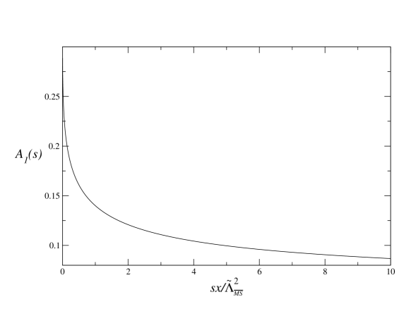
Figure 1: The function ${A}_{1}(s)$ of Eq.(19) versus $sx/{\tilde{\Lambda}}_{\overline{MS}}^{2}$. We assume ${N_{f}}=2$ flavours of quark.

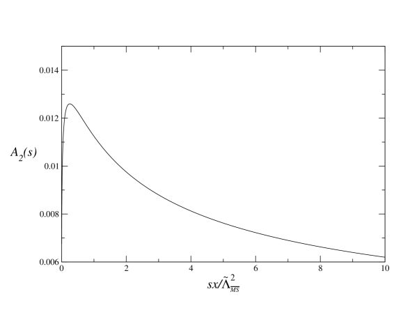
Figure 2: As Fig.1 but for ${A}_{2}(s)$ of Eq.(20).

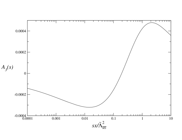
Figure 3: As Fig.1 but for ${A}_{3}(s)$ of Eq.(20).

We have shown that the freezing occurs to all-orders in perturbation theory, and thus must occur independent of the choice of renormalization scheme. The use of a ’t Hooft scheme turns out to make the freezing manifest. We used a general choice of renormalization scale ${\mu}^{2}=xs$. The true infra-red $s$-dependence of ${\cal{R}}(s)$ does not depend on the unphysical parameter $x$. One should rather eliminate the ${\mu}$-dependence of the result altogether by completely resumming all the ultra-violet logarithms which build the $s$-dependence. This so-called Complete Renormalization Group Improvement (CORGI) approach [20] corresponds to choosing ${\mu}^{2}={e}^{-2d/b}s$, where $d$ is the NLO perturbative correction $d_{1}$ to ${\cal{D}}(s)$ in Eq.(5), in the $\overline{MS}$ scheme with ${\mu}^{2}=s$. One then has the “contour-improved” CORGI series,

$${\cal{R}}(s)={A}_{1}(s)+{\sum_{n=2}^{\infty}}{X}_{n}{A}_{n+1}(s)\;,$$ (21)

where the $X_{n}$ are the CORGI invariants, and only $X_{2}$ is known. Now $A(s)=(-1/e){({\sqrt{s}}/{\Lambda}_{D})}^{-b/c}$, where ${\Lambda}_{D}{\equiv}{e}^{d/b}{\tilde{\Lambda}}_{\overline{MS}}$. For an infra-red fixed point at ${\cal{R}}(0)={\cal{R}}^{\ast}$, corresponding to a zero of the beta-function, one expects the asymptotic behaviour [2]

$${\cal{R}}(s)-{\cal{R}}^{\ast}{\sim}{s}^{\gamma}\;,$$ (22)

where $\gamma$ is a critical exponent. Our freezing to $2/b$ is instead driven by the analytical continuation from the Euclidean to Minkowskian regions, and one obtains the asymptotic behaviour,

$${\cal{R}}(s)-\frac{2}{b}{\approx}\frac{-1/c-2/b}{{W}_{0}(-A(s))}\;.$$ (23)

Again this involves the ubiquitous Lambert $W$ function.

We should stress that, of course, the result ${\cal{R}}(0)=2/b$ is in itself only of abstract interest since $s=4{m}_{\pi}^{2}$ is the threshold in full QCD with massive quarks. The important conclusion is that while the conventional perturbation series of Eq.(2) breaks down at the spurious Landau pole in the coupling $a(s)$, this is eliminated by completely resumming all the analytical continuation terms, so that the “contour-improved” (or APT) perturbation series is well-behaved in the infra-red. It was crucial in investigating this to be able to evaluate the functions ${A}_{n}(s)$ in closed analytic form. In previous phenomenological investigations [9, 10] these functions were evaluated by numerical integration with Simpson’s Rule, making it impossible to go further into the infra-red than the Landau pole obstruction. Whilst the infra-red freezing is most easily investigated using the “contour improved” or Analytic version of the perturbation series in Eqs.(8,21), it should be stressed that the freezing is an all-orders result of QCD perturbation theory. The standard expectation is that by itself the all-orders perturbation series is ambiguous due to the presence of infra-red renormalons, these renormalon ambiguities cancelling against corresponding non-logarithmic UV divergences in the non-perturbative Operator Product Expansion (OPE) [21]. The vanishing of the ${A}_{n}(s)$ for $n>1$ in the infra-red means that these renormalon ambiguities also vanish, and so the implication is that the non-logarithmic UV divergences of the OPE also vanish in the infra-red. This of course says nothing about the infra-red limit of the resummed OPE, indeed we know that there are important non-perturbative effects which build a complicated set of hadronic resonances, but the interesting observation is that perturbative and non-perturbative effects are separately well-defined in the infra-red limit for Minkowskian quantities. This is not the case for Euclidean quantities where the Euclidean APT coupling necessarily includes a resummation of non-perturbative OPE terms [12].

There are evidently many phenomenological applications of the “contour-improved” CORGI perturbation series for ${\cal{R}}(s)$, in particular one can repeat the analysis of Ref.[2] and compare PQW smeared [5] data for ${R}_{{e}^{+}{e}^{-}}(s)$ with the similarly smeared perturbative freezing. This exercise has been performed in the APT approach in Ref.[22], and good agreement found. There will also be applications to estimating uncertainties in ${\alpha}(M_{Z})$, and in estimating the hadronic corrections to the anomalous magnetic moment of the muon. We hope to report on these aspects in a future publication.

References

- [1] For a recent comprehensive review see: S. Bethke, J. Phys. G 26 (2000) R27.
- [2] A.C. Mattingly and P.M. Stevenson, Phys. Rev. D49 (1994) 437.
- [3] J.M. Cornwall Phys. Rev. D26 (1982) 1453; G. Parisi and R. Petronzio, Phys. Lett. B94 (1980) 51.
- [4] Y.L. Dokshitzer, G. Marchesini and B.R. Webber, Nucl. Phys. B469 (1996) 93.
- [5] E.C. Poggio, H.R. Quinn and S. Weinberg, Phys. Rev. D13 (1976) 1958.
- [6] J. Chyla, A. Kataev and S. Larin, Phys. Let. B267 (1991) 269.
- [7] S.G. Gorishny, A.L. Kataev and S.A. Larin, Phys. Lett. B212 (1988) 238.
- [8] L.R. Surguladze and M.A. Samuel, Phys. Rev. Lett. 66, (1990) 560; S.G. Gorishny, A.L. Kataev and S.A. Larin, Phys. Lett. B259 (1991) 144.
- [9] A.A. Pivovarov, Sov. J. Nucl. Phys. 54 (1991) 676; A.A. Pivovarov, Z. Phys. C53 (1992) 461.
- [10] F. Le Diberder and A. Pich, Phys. Lett B289 (1992) 165.
- [11] D.J. Broadhurst, A.L. Kataev and C.J. Maxwell, Nucl. Phys. B592 (2001) 247.
- [12] D.V. Shirkov, Eur. Phys.J.22 (2001) 331.
- [13] G ’t Hooft, in Deeper Pathways in High Energy Physics, proceedings of Orbis Scientiae, 1977, Coral Gables, Florida, edited by A. Perlmutter and L.F. Scott (Plenum, New York, 1977).
- [14] E. Gardi, G. Grunberg and M. Karliner, JHEP 07 (1998) 007.
- [15] P.M. Stevenson, Phys. Rev. D23 (1981) 2916.
- [16] A.J. Buras, E.G. Floratos, D.A. Ross and C.T. Sachrajda, Nucl. Phys. B131 (1977) 308.
- [17] R.M. Corless, G.H. Gonnet, D.E.G Hare, D.J. Jeffrey and D.E. Knuth, “On the Lambert function”, Advances in Computational Mathematics 5 (1996) 329, available from http://www.apmaths.uwo.ca/djeffrey/offprints.html.
- [18] C.J. Maxwell and A. Mirjalili, Nucl. Phys. B611 (2001) 423.
- [19] B.A. Magradze, “The QCD coupling up to third order in standard and analytic perturbation theories.”, hep-ph/0010070; D.S. Kourashev and B.A. Magradze, “Explicit expressions for Euclidean and Minkowskian observables in analytic perturbation theory” hep-ph/0104142 (to appear in Theor. Math. Phys.).
- [20] C.J. Maxwell and A. Mirjalili, Nucl. Phys. B577 (2000) 209; S.J. Burby and C.J. Maxwell, Nucl. Phys. B609 (2001) 193.
- [21] For a review see: M. Beneke and V.M. Braun, hep-ph/0010208, published in “The Boris Ioffe Festschrift- At the Frontier of Particle Physics/Handbook of QCD”, edited by M. Shifman (World Scientific, Singapore, 2001).
- [22] D.A. Shirkov and I. Solovtsov, hep-ph/9906495; published in “Proceedings of the International Workshop on collisions”, Eds. G. Fedotovich and S. Redin, Novosibirsk 2000, pp. 122-124.