HIP-2002-10/TH

NORDITA-2002-20-HE

hep-ph/0204034

3 April, 2002

RAPIDITY DEPENDENCE OF PARTICLE PRODUCTION IN ULTRARELATIVISTIC NUCLEAR COLLISIONS

K.J. Eskola^a,c,, K. Kajantie^b,c,, P.V. Ruuskanen^a,c, and K. Tuominen^d,

^a Department of Physics, University of Jyväskylä,
P.O. Box 35, FIN-40351 Jyväskylä, Finland
^b Department of Physics,
P.O. Box 64, FIN-00014 University of Helsinki, Finland
^c Helsinki Institute of Physics,
P.O. Box 64, FIN-00014 University of Helsinki, Finland
^d Nordita,
Blegdamsvej 17, 2100 Copenhagen Ø, Denmark

Abstract

We compute the rapidity dependence of particle and transverse energy production in ultrarelativistic heavy ion collisions at various beam energies and atomic numbers using the perturbative QCD + saturation model. The distribution is a broad gaussian near $y=0$ but the rapid increase of particle production with the beam energy will via energy conservation strongly constrain the rapidity distribution at large $y$.

1 Introduction

The Relativistic Heavy Ion Collider RHIC has already produced a lot of data at $\sqrt{s}$ up to 200 GeV and the planning for the ALICE/Large Hadron Collider experiment at $\sqrt{s}$ up to 5500 GeV is under way. The first data are on various large cross section phenomena like charged multiplicity at zero (pseudo)rapidity in nearly central collisions [1, 2] or at varying [3, 4] impact parameter, or as a function of both rapidity and centrality [5, 6]. Much theoretical effort, reviewed in [7], has been devoted both to predict the multiplicities before measurements and to draw conclusions from the completed measurements. With this information the reliability of predictions for the LHC energies, $\sqrt{s}=5500$ GeV, is considerably enhanced.

One of the models, reasonably successful in predicting the data at RHIC energies, is the saturation+pQCD model [8], based on microscopic 2$\to$2 partonic processes. It is actually a member of a large class of models in which there is one dominant transverse momentum scale, $p_{{\mbox{\scriptsize sat}}}$, determined by different versions of a saturation condition [9, 10, 11, 12, 13]. The purpose of this note is to apply the model to a study of the rapidity dependence of particle and transverse energy production. Related work in [14] and [15], based on microscopic 2$\to$1 processes, will be compared with.

The main observation is that, not surprisingly, energy conservation places strong constraints [16] to the domain of validity of models based on independent 2$\to$2 subcollisions. There is no problem at zero rapidity: $N(y=0)$ and $E_{T}(y=0)$ grow rapidly with $\sqrt{s}$, but still much more slowly that the total available energy $\sqrt{s}$. At larger rapidities such a rapid growth of $N(y)$ cannot be sustained, the total energy carried by the produced particles would surpass the available total energy indicating that one has entered a new domain in which the independent scattering model no more is valid. We estimate that at RHIC the saturation+pQCD model could be valid up to $y=1...2$, and at LHC up to $y=3...4$. Within this range the rapidity distribution is very flat, practically a wide gaussian with calculable curvature near $y=0$. This is in marked contrast to the $2\to 1$ model in [14, 15], where $N(y)$ is sharply peaked at $y=0$, in fact, has a discontinuous derivative there.

2 Rapidity dependence in the saturation + pQCD model

We shall first carry out an approximate analytic discussion emphasizing parametric dependences. One starts from the perturbatively determined leading-order two-jet cross section (in standard notation):

$$\frac{d\sigma^{AA\rightarrow kl+X}_{\rm pQCD}}{dp_{T}^{2}dy_{1}dy_{2}}=K\sum_{ij}\,x_{1}f_{i/A}(x_{1},p_{T}^{2})\,x_{2}f_{j/A}(x_{2},p_{T}^{2})\,\sum_{kl}\frac{d\hat{\sigma}}{d\hat{t}}^{ij\rightarrow kl}.$$ (1)

To maintain the framework of [8], we use the GRV94 leading-order parton distribution functions [17, 18] combined with the nuclear effects (shadowing) from the EKS98 parametrization [19]. An effective factor $K\approx 2$ is to simulate the NLO contributions which are discussed in more detail in [20]. After integration over $y_{2}$ Eq. (1) gives a single-jet cross section behaving near the dominant saturation scale (which depends on $\sqrt{s}$ and $A$, and also on $y$) parametrically like [21]

$${d\sigma_{\rm pQCD}\over dyd^{2}p_{T}}\sim\sqrt{s}^{\,2\delta}{\alpha_{s}^{2}(p_{T}^{2})\over p_{T}^{4}}e^{-y^{2}/2\sigma^{2}(p_{T})},$$ (2)

where $\delta\approx 0.5$ (when no shadowing is included) and the $y$-dependence has been approximated by a gaussian (the letter $\sigma$ is used for both the cross section and the width of the gaussian). A further integration over $p_{T}$ from some lower limit gives the hard cross section (see Figs. 2 and 3 below)

$$\frac{d\sigma_{\rm pQCD}}{dy}(p_{0})\sim\sqrt{s}^{\,2\delta}{\alpha_{s}^{2}(p_{0}^{2})\over p_{0}^{2}}e^{-y^{2}/2\sigma^{2}(p_{0})}.$$ (3)

Consider now central A+A collisions with the nuclear overlap function $T_{AA}(b=0)=A^{2}/(\pi R_{A}^{2})$. The saturation condition then can be formulated as

$$\frac{dN}{dy}(p_{0}) = {A^{2}\over\pi R_{A}^{2}}\frac{d\sigma_{\rm pQCD}}{dy}(p_{0})=p_{0}^{2}R_{A}^{2}$$

$$\sim {A^{2}\over\pi R_{A}^{2}}\sqrt{s}^{\,2\delta}{\alpha_{s}^{2}(p_{0}^{2})\over p_{0}^{2}}e^{-y^{2}/2\sigma^{2}(p_{0})},$$

the solution of which gives $p_{0}=p_{{\mbox{\scriptsize sat}}}(A,\sqrt{s},y)$. The saturation is here defined as the geometric saturation on the transverse plane of the two final state particles in the 2$\to$2 collision. The $2\to 1$ models describe saturation as the separate saturation of the distribution functions of the two initial state particles. As long as there is one dominant tranverse momentum scale, the models lead to similar results, at least when final state particle production in nearly central collisions is considered.

The principle underlying the saturation condition is illustrated by Fig. 1. The perturbative cross sections, of course, are valid only for large $p_{T}$. However, one is only interested in the integral over $p_{T}$, not the value of the distribution at small $p_{T}$. The value of the full integral can also be reproduced by integrating the perturbative distribution from a lower limit given by the saturation condition.

                 

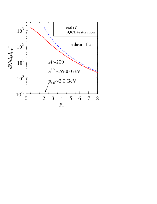
Figure 1: The qualitative $p_{T}$ distribution of gluons produced in a heavy ion collisions at $\sqrt{s}=5500$ GeV (solid curve). Only the integral over $p_{T}$ has physical meaning; the saturation+pQCD model produces the same integral by integrating over the dashed curve computed using pQCD but with the lower limit determined by the saturation condition (2).

To approximately solve Eq. (2) for $p_{0}=p_{{\mbox{\scriptsize sat}}}$ one may neglect the $p_{0}$-dependence of $\sigma$ and approximate $\alpha_{s}^{2}(p_{0})\sim 1/p_{0}^{2\xi},\,\,\xi\approx 0.44$. This numerical value actually contains also a contribution from the $p_{T}$-integration [21]. Then,

$$p_{{\mbox{\scriptsize sat}}}(y) \sim A^{1/(6+3\xi)}\sqrt{s}^{\,\delta/(2+\xi)}e^{-y^{2}/(4(2+\xi)\sigma^{2})}$$ (5)

$$\sim 0.208\,{\rm GeV}A^{0.128}\sqrt{s}^{\,0.191}e^{-y^{2}/(4(2+\xi)\sigma^{2})},$$ (6)

$$dN/dy \sim A^{(6+2\xi)/(6+3\xi)}\sqrt{s}^{\,2\delta/(2+\xi)}e^{-y^{2}/(2(2+\xi)\sigma^{2})}$$ (7)

$$\sim 1.383A^{0.922}\sqrt{s}^{\,0.383}e^{-y^{2}/(2(2+\xi)\sigma^{2})},$$ (8)

where the numerical values computed in [8] with shadowing are also given.

The scaling exponents of $A$ and $\sqrt{s}$ are the ones from [8, 21]; the rapidity dependence is new. Note how the saturation condition leads to $N\sim A^{a},\,a\approx 1$ [11], though in the independent collision limit $N\sim A^{4/3}$. Similarly, the saturation condition has a significant effect on the rapidity distribution of saturated particle production: it is wider than that of elementary subprocesses by a factor $\sqrt{2+\xi}\approx 1.6$.

In the numerical computation, one first evaluates $dN/dy(p_{0})=T_{AA}(0)d\sigma_{\rm pQCD}/dy(p_{0})$, The result is shown in Fig. 2 together with a gaussian fit $\sim\exp(-y^{2}/(2\sigma^{2}))$. The distributions get narrower when $p_{0}$ increases: at $\sqrt{s}=5500$ GeV $\sigma(p_{0})\approx 6.6-p_{0}$.

     

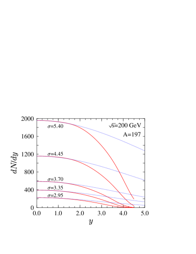
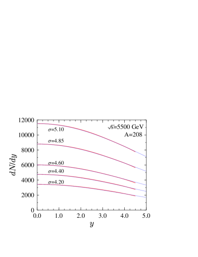
Figure 2: Plots of $dN/dy=T_{AA}(0)d\sigma_{\rm pQCD}/dy(p_{0})$ for $\sqrt{s}=200$ GeV (from top to bottom $p_{0}=1.0,1.2,1.5,1.7,2.0$ GeV) and 5500 GeV (from top to bottom $p_{0}=1.5,1.7,2.0,2.2,2.5$ GeV). The dashed lines show a gaussian fit $\sim\exp(-y^{2}/(2\sigma^{2}))$.

Using the numerically computed $dN/dy(p_{0})$ the saturation condition operates as shown in Fig. 3 and leads to $N_{AA}(y)$ also in Fig. 3. In agreement with the analytic argument in Eq. (8) a very broad distribution near $y=0$ is obtained:

$$\sigma = 5.8\qquad\sqrt{s}=130\,\,\,{\rm GeV},$$ (9)

$$= 5.9\qquad\sqrt{s}=200\,\,\,{\rm GeV},$$ (10)

$$= 6.8\qquad\sqrt{s}=5500\,{\rm GeV}.$$ (11)

     

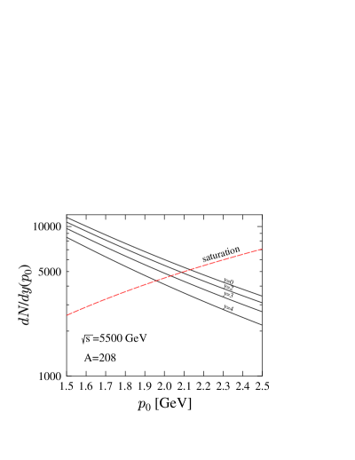
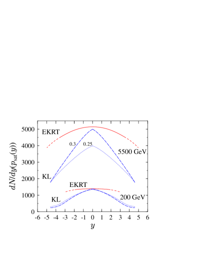
Figure 3: The left panel shows how the saturation condition (2) operates: the dashed line shows its RHS $p_{0}^{2}R_{A}^{2}$, the solid lines show the LHS $T_{AA}(0)d\sigma_{\rm pQCD}(p_{0},y)/dy$ at $\sqrt{s}=5500$ GeV for various $y$ as a function of $p_{0}$. The point of intersection gives both the value of $p_{{\mbox{\scriptsize sat}}}(y)$ and of $dN/dy(p_{{\mbox{\scriptsize sat}}}(y))$, the value of which is plotted in panel at right for central Pb-Pb collisions at $\sqrt{s}=5500$ GeV and Au-Au at 200 GeV. The dotted and dashed curves show the prediction of [14] for $\lambda=0.25,\,0.3$ respectively.

The form of the rapidity dependence of the saturation scale proposed in [14, 15] is markedly different. One first notes that the conjectured saturation scale as determined from deep inelastic scattering [22] can be parametrised as

$$Q_{s}^{2}(x)=Q_{0}^{2}\left({x_{0}\over x}\right)^{\lambda},$$ (12)

where $Q_{0}\approx$ 1 GeV, $x_{0}\approx 3\cdot 10^{-4}$ and $\lambda\approx 0.3$. To relate the DIS Bjorken variable $x$ to the A+A gluon production variables, one further writes that $x\sim e^{y-y_{B}}$. Then $Q_{s}^{2}(y)\sim\sqrt{s}^{\lambda}e^{-\lambda|y|}$. Including only the region in which both initial gluons in the 2$\to$1 process are saturated, one obtains

$${dN\over dy}\sim Q_{s}^{2}(y)\sim\sqrt{s}^{\lambda}e^{-\lambda|y|}.$$ (13)

Thus the rapidity distribution will have a sharp peak at $y=0$, as shown in the right panel of Fig. 3. In Ref. [14] it is assummed that the pseudorapidity distribution of produced gluons (virtual, $m_{g}^{2}\approx Q_{s}\cdot 1$ GeV, $p_{T}\approx Q_{s}$) directly give the pseudorapidity distributions of pions in the final state, apart from a multiplicative normalization factor $c$. Thus $dN_{\rm ch}/d\eta\approx c\cdot dN_{g}/d\eta$, where $c$ contains factors from the actual gluon production, such as the gluon liberation constant $c_{g}={\cal O}(1)$ and possible factors related to the normalization and approximations made for the unintegrated gluon densities. The constant $c$ also includes factors related to hadronization, decays and particle content in the final state. Such factors are $c_{\pi/g}$ which indicates how many pions come from each virtual gluon, and a factor $c_{\rm ch}$ accounting for the conversion of total to charged multiplicity. It should be noted that when plotting the rapidity distributions of [14] for the produced gluons in Figs. 3 (right panel) and in Fig. 5 (left panel), we have fixed the normalization constant $c=c_{\rm ch}\cdot c_{\pi/g}\cdot c_{g}$ based on the measured $dN_{\rm ch}/d\eta$ [5], and used $c_{\rm ch}\approx 2/3$. As our primary goal here is to compare the shapes of the rapidity spectra of the two approaches, we have not tried to undo the effect of the factor $c_{\pi/g}$. As the virtuality of the produced gluons in [14] is taken to be larger than $m_{\rho}$, we expect that the actual number of initially produced gluons in the saturation model of [14] can be down by $c_{\pi/g}\sim 2$ relative to what is shown in Figs. 3 and 5.

One may observe that in the final state saturation calculation one does not at all need the distribution functions within the saturation region as defined by Eq. (12). To check the effect of saturated distribution functions on the 2$\to$2 model one can perform the following computation. Including only the dominant gluons one has

$${d\sigma\over dyd^{2}p_{T}}\approx K\int dy_{2}\,x_{1}g(x_{1},p_{T}^{2})\,x_{2}g(x_{2},p_{T}^{2}){9\alpha_{s}^{2}\over 2p_{T}^{4}},$$ (14)

where $x_{1}=p_{T}/\sqrt{s}\cdot(e^{y}+e^{y_{2}}),\,\,x_{2}=p_{T}/\sqrt{s}\cdot(e^{-y}+e^{-y_{2}})$. A simple model for saturated distribution functions (see [14]) would be

$$xg(x,p_{T}^{2})=C{S_{A}\over\alpha_{s}}\left\{p_{T}^{2}\cdot\Theta\left[Q_{0}^{2}({x_{0}\over x})^{\lambda}-p_{T}^{2}\right]+Q_{0}^{2}({x_{0}\over x})^{\lambda}\Theta\left[p_{T}^{2}-Q_{0}^{2}({x_{0}\over x})^{\lambda}\right]\right\}$$ (15)

with $S_{A}\approx\pi R_{A}^{2}$, $C$ = constant, and where implicitly $Q_{0}^{2}\sim A^{1/3}$. Integration over $y_{2}$ and $p_{T}$ then gives a $y$-distribution which is broad and very similar to those in Figs. 2 and 3. We thus conclude that the broad $y$-distribution is not due to the use of distributions in the DGLAP region, it is a property of the 2$\to$2 model as such.

The $\sqrt{s}$ and $y$ dependences of the result (13) are sensitive to the value of the parameter $\lambda=0.25\dots 0.30$, especially when one approaches LHC energies. Furthermore this $\lambda$ interval is based on the analysis in Ref. [22] which neglects the scale evolution of the gluon distribution in the non-saturated region on which the saturated gluon distribution has to be matched in the vicinity of the ’critical line’ $Q_{s}^{2}(x)$ defining the transition region from saturated to non-saturated gluon densities. An interesting recent analysis in [23] suggests that one might be led to consider values as large as $\lambda\sim 0.5$. This is similar to the behaviour of the gluon distribution at the final state saturation scale [21].

3 Energy conservation

The results (5)-(8) lead to a rather striking powerlike growth with energy, especially for the transverse energy $\sim p_{{\mbox{\scriptsize sat}}}(y)N(y)$. Let us thus estimate when the total amount of energy within some rapidity range $-y_{\mbox{\scriptsize up}}<y<y_{\mbox{\scriptsize up}}$ is less than some fraction, 40%, say, of the total energy $A\sqrt{s}\approx Ae^{y_{\mbox{\scriptsize B}}}$ available (GeV units are used), neglecting first the weak rapidity dependence. A simple analytic estimate of this is ($c_{N},c_{p}$ are the constants in (6),(8)):

$$E(|y|\leq y_{\mbox{\scriptsize up}}) \approx \int_{-y_{\mbox{\scriptsize up}}}^{y_{\mbox{\scriptsize up}}}dy\frac{dN}{dy}\bigg{|}_{y=0}p_{{\mbox{\scriptsize sat}}}(y=0)\cosh y\approx\frac{dN}{dy}\bigg{|}_{y=0}p_{{\mbox{\scriptsize sat}}}(0)e^{y_{\mbox{\scriptsize up}}}$$

$$\approx c_{N}c_{p}A^{(7+2\xi)/(6+3\xi)}\sqrt{s}^{\,3\delta/(2+\xi)}e^{y_{\mbox{\scriptsize up}}}<0.4A\sqrt{s}$$

giving

$$y_{\mbox{\scriptsize up}}+\log(c_{N}c_{p}A^{(1-\xi)/(6+3\xi)})<y_{B}(1-{3\delta\over 2+\xi})+\log 0.4.$$ (17)

The two logs are constants of order one, but the qualitatively important factor is $y_{B}(1-3\delta/(2+\xi))\approx y_{B}(1-0.62)$; it expresses the fact that with increasing beam energy particle production in the saturation + pQCD model will exhaust the total available energy within a fixed fraction of the beam rapidity $y_{B}$. Beyond that rapidity this independent subcollision model cannot be valid and the physical mechanism has to change completely. The same effect is shown more quantitatively in Fig. 4, where we have computed the total produced energy as

$$E(y_{\rm up})=\int_{-y_{\rm up}}^{y_{\rm up}}dy\int_{p_{{\mbox{\scriptsize sat}}}(y)}dp_{T}\frac{dN}{dp_{T}dy}\cdot p_{T}\cosh y,$$ (18)

The rapidity distributions of produced partons are obtained from Eq. (1), as discussed in detail in Ref. [24]. Keeping the saturation scale fixed at $p_{{\mbox{\scriptsize sat}}}(y=0)$ gives the dotted lines, not qualitatively different from the solid lines obtained with the rapidity dependent saturation.

Figure 4: The total energy produced in the saturation + pQCD model up to $|y|<y_{\mbox{\scriptsize up}}$ relative to the cms-energy in central $AA$ collisions. The cms-energies and nuclei are denoted in the figure. “Initial” refers to time after formation before any collective expansion. The solid curves are computed from Eq. (18) with $p_{{\mbox{\scriptsize sat}}}(y)$, and the dotted curves with a fixed $p_{{\mbox{\scriptsize sat}}}(y=0)$ as the lower limit of $p_{T}$-integration.

The saturation+pQCD model thus predicts that the $y$-distribution $N(y)$ is very flat, gaussianlike around $y=0$, with height increasing as given by Eq. (8) but extending only up to some maximum value of $y$ imposed by energy conservation. We emphasize that the saturation condition itself leads to a broadening of the rapidity distribution. Allowing 40% of the total energy leads to $|y|\raise 1.29167pt\hbox{$<$\kern-7.5pt\raise-4.73611pt\hbox{$\sim$}}2$ at RHIC (with $y_{B}=4.93$ (5.36) for $\sqrt{s}=$ 130 (200) GeV) and $|y|\raise 1.29167pt\hbox{$<$\kern-7.5pt\raise-4.73611pt\hbox{$\sim$}}3.5$ at LHC (with $y_{B}=8.67$). Beyond these values correlations between subcollisions must start to play an increasingly important role.

4 Hydrodynamic evolution

The previous considerations apply at the initial time $\tau_{i}(y)\approx 1/p_{{\mbox{\scriptsize sat}}}(y)$. Within the domain of validity, $|y|<y_{\mbox{\scriptsize up}}$, there is little variation in $\tau_{i}(y)$. Hydrodynamic evolution in the case of $y$-dependent initial conditions of the type obtained here was numerically studied in [25]. There is always significant flow of $E_{T}$ from small to large rapidities, due to $pdV$ work [8, 26], but in this $y$-dependent case there is also some flow of entropy from small to large rapidities. Typically, the entropy density at $y=0$ decreases by about 10%, as shown in [25].

We thus conclude that the time evolution of $y$-distribution is one more detail to be added to the list of factors affecting the relation between initial and final multiplicity [26]: initial and final particle-to-entropy ratios, charged-to-neutral ratio, transverse expansion, equation of state, decoupling effects and resonance decays. However, in the central region the hydrodynamic evolution affects only the overall magnitude of the rapidity distribution while the effect on the shape is small.

5 Comparison with RHIC data

We note first that the RHIC data [5, 6] gives the pseudorapidity distribution $dN_{\rm ch}/d\eta$ while our computations so far are for $dN/dy$ at the moment of formation of the partonic system. The conversion of $N$ to the observed $N_{\mbox{\scriptsize ch}}$ is simple (see end of previous section), but the relation between $y$- and $\eta$-distributions is more subtle [26].

The rapidity distribution of particles is the sum

$$\frac{dN}{dy}\equiv\int dp_{T}\sum_{i}\frac{dN_{i}}{dp_{T}dy},$$ (19)

where the index $i$ runs through all particles included in the spectrum, similarly for pseudorapidity. We have shown explicitly the transverse momentum integration to emphasize that the connection between the rapidity and pseudorapidity depends on the mass and the transverse momentum of particles: $y={\rm arsinh}((p_{T}/m_{Ti})\sinh\eta)$. Similarly the Jacobian

$$J_{i}(\eta,p_{T},m_{i})=\frac{\partial y}{\partial\eta}=\frac{p}{E_{i}}$$ (20)

in the transformation between the spectra

$$\frac{dN}{d\eta}\equiv\int dp_{T}\frac{dN}{dp_{T}d\eta}=\int dp_{T}\sum_{i}J_{i}(\eta,p_{T},m_{i})\frac{dN_{i}(p_{T},y)}{dp_{T}dy},$$ (21)

depends on the mass and the transverse momentum. In the following we will assume that pions dominate and consider equations for single particle only.

The pseudorapidity data [5] is characterized by a dip in a central plateau of total extent of 3…4 in $\eta$. Starting from a flat rapidity distribution, this dip results from the Jacobian in the transformation to pseudorapidity. The depth of the dip is quite sensitive to particle masses and shapes of the transverse momentum and rapidity distributions, variations by a factor two in the depth of the dip can easily take place. We also emphasize the difference between performing the transformation using Eq. (21) with $p_{T}$ and $y$ distributions or simply approximating the Jacobian by $dN/d\eta=J(\eta,\langle p_{T}\rangle,m)dN/dy$.

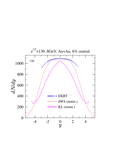
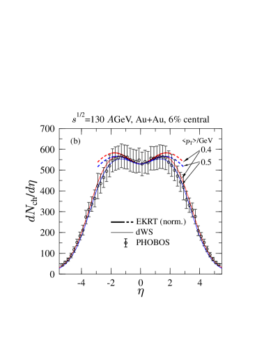
Figure 5: (Left) Initial rapidity distributions $dN/dy$ for the saturation+pQCD model (solid curve, EKRT), for the double-Woods-Saxon (dWS) parametrization (22) (dotted curve) and for the prediction of [14] (dashed curve) (see text). (Right) The final state pseudorapidity distributions $dN/d\eta$ (6% central): data [1], the saturation + pQCD model (thick solid lines, EKRT) and the parametrisation (22) (see text).

In Fig. 5a the results from calculations of the initial $dN/dy$ are shown for nearly central Au+Au collisions at $\sqrt{s}=130$ GeV. The solid curve (EKRT) is the prediction with $y$-dependent saturation of produced partons, computed as in Figs. 3. A 6% centrality cut corresponds to an effective nucleus $A=178$, as discussed in [26]. Within the dashed part of the curve more than 40% of total energy has been consumed (Fig. 4); the curves stop when all the energy is consumed. The dotted curve shows a double-Woods-Saxon (dWS) parametrization

$${dN\over dy}=N(0)\frac{(1+e^{-y_{0}/d})^{2}}{(1+e^{(-y-y_{0})/d})(1+e^{(y-y_{0})/d})}\,,$$ (22)

normalised to the EKRT result at $y=0$. Here $y_{0}=3.3$ gives the width of the distribution and $d=0.65$ the steepness at this cutoff. This double Woods-Saxon form for $dN/dy$ is an arbitrary parametrization designed to reproduce the pseudorapidity data [5] but it has the two elements we want to emphasize, the flatness of $dN/dy$ at small rapidities and the rapid decrease at large values of $y$ required by energy conservation. Finally, the dashed curve is the initially produced rapidity distribution from [14]. The normalization of this curve was discussed in the end of Sec. 2.

Fig. 5b shows the data [5] with $dN_{\rm ch}/d\eta$ curves calculated from $dN/dy$ assuming that all particles are pions with an exponential transverse momentum distribution, $dN/dp_{T}^{2}dy\sim dN/dy\cdot\exp(-2p_{T}/\langle p_{T}\rangle)$, with $\langle p_{T}\rangle=0.4$ GeV or 0.5 GeV. The thick solid lines (EKRT) are the saturation model prediction, computed using Eq. (21). The dashed parts of the lines correspond to those in the left panel and indicate again where energy conservation is expected to suppress the distributions. The thin solid lines (dWS) are from the parametrization (22) with $y_{0}=3.3$ and $d=0.65$, which reproduce the PHOBOS data. In the framework of [8], the initial and final state rapidity distributions are connected through entropy conservation by $dN_{ch}/dy=2/3\cdot 3.6/4.0\cdot dN/dy(p_{{\mbox{\scriptsize sat}}}(y))$. Here, in order to study the shapes of the obtained spectra, all the curves are normalized to the same point at $\eta=0$. Compared with the normalization in [8], an additional factor 0.95 (0.92) for $\langle p_{T}\rangle=0.4$ (0.5) GeV is applied to the EKRT curves in Fig. 5b. The relation between the initial and final multiplicities is studied in more detail in [26].

We do not show here the pseudorapidity distribution from the dashed curve in the left panel; in [14] the $y\to\eta$ transformation was carried out simply using a Jacobian $J(\eta,p_{T},m_{g})$, calculated for virtual gluons with $m_{g}^{2}\approx Q_{s}\cdot 1$ GeV and $p_{T}\approx Q_{s}$, as a multiplicative factor between $dN/dy$ and $dN/d\eta$. With $Q_{s}(y=0)=\sqrt{2}$ GeV [27] the suppression from the $y$- to $\eta$- distribution at $y=\eta=0$ is $p_{T}/m_{T}\approx 0.76$, which turns the peak in the $y$ distribution into a dip in the $\eta$-distribution. The results of [14] are thus very close to the data in Fig. 5b.

6 Conclusions

We have discussed the rapidity distribution $dN/dy$ of particles produced in very high energy central $A+A$ collisions in the saturation+pQCD model. The distribution around $y=0$ will be a broad gaussian with a calculable width and with the value $dN/dy(y=0)$ increasing rapidly, powerlike. However, the model can be applied only until some value $y_{\mbox{\scriptsize up}}$ ($\approx$ 1…2 at RHIC, 3…4 at LHC), beyond which some new type of fragmentation region dynamics, taking into account correlations between subcollisions, must enter. At asymptotic energies the saturation region is parametrically favoured by powers of $1/\alpha_{s}$ and this will damp the distribution at large $y$.

The overall magnitude of $dN/d\eta$ at $\eta=0$ predicted by the saturation + pQCD model agreed very well with RHIC experiments for central collisions. The centrality dependence was also reproduced on the 10% level within $N_{\rm part}\raise 1.29167pt\hbox{$<$\kern-7.5pt\raise-4.73611pt\hbox{$\sim$}}100$. A more reliable calculation on the $y$-dependence of initial gluon production can be made only after a better understanding of the correlations among subprocesses in the fragmentation and near fragmentation regions has been achieved. At present one may note that within the domain of validity of the model, before energy conservation makes the assumption of independent subcollisions invalid, there is agreement with data. The width of the relevant $y$-range at RHIC is narrow, but becomes appreciable at LHC energies. It will be very interesting to see how a rapid increase at $y=0$ and dynamics in the fragmentation regions will be related.

Acknowledgements We thank M. Gyulassy for suggesting this computation many years ago, and D. Kharzeev and N. Armesto for discussions. Financial support from the Academy of Finland (grants No. 163065, 77744 and 50338) is gratefully acknowledged.

References

- [1] B. B. Back et al. [PHOBOS Collaboration], Phys. Rev. Lett. 85 (2000) 3100 [hep-ex/0007036].
- [2] B. B. Back et al. [PHOBOS Collaboration], nucl-ex/0108009.
- [3] K. Adcox et al. [PHENIX Collaboration], Phys. Rev. Lett. 86 (2001) 3500 [nucl-ex/0012008].
- [4] B. B. Back et al. [PHOBOS Collaboration], “Centrality dependence of charged particle multiplicity at mid-rapidity in Au + Au collisions at s(NN)**(1/2) = 130-GeV,” nucl-ex/0105011.
- [5] B. B. Back et al. [PHOBOS Collaboration], Phys. Rev. Lett. 87 (2001) 102303 [nucl-ex/0106006].
- [6] I. G. Bearden et al. [BRAHMS Collaboration], “Pseudorapidity distributions of charged particles from Au + Au collisions at the maximum RHIC energy,” nucl-ex/0112001.
- [7] K. J. Eskola, Nucl. Phys. A 698 (2002) 78 [hep-ph/0104058].
- [8] K. J. Eskola, K. Kajantie, P. V. Ruuskanen and K. Tuominen, Nucl. Phys. B570 (2000) 379 [hep-ph/9909456].
- [9] L.V. Gribov, E.M. Levin and M.G. Ryskin, Phys. Rept. 100 (1983) 1.
- [10] A.H. Mueller and J. Qiu, Nucl. Phys. B268 (1986) 427.
- [11] J. P. Blaizot and A. H. Mueller, Nucl. Phys. B289 (1987) 847.
- [12] M. Gyulassy and L. McLerran, Phys. Rev. C 56 (1997) 2219 [nucl-th/9704034].
- [13] Xiaofeng Guo, Phys. Rev. D 59 (1999) 094017 [hep-ph/9812257].
- [14] D. Kharzeev and E. Levin, Phys. Lett. B 523 (2001) 79 [nucl-th/0108006].
- [15] D. Kharzeev, E. Levin and M. Nardi, “The onset of classical QCD dynamics in relativistic heavy ion collisions,” hep-ph/0111315.
- [16] H. J. Drescher, M. Hladik, S. Ostapchenko, T. Pierog and K. Werner, New Jour. Phys. 2 (2000) 31 [hep-ph/0006247].
- [17] M. Glück, E. Reya and A. Vogt, Z. Phys. C67 (1995) 433.
- [18] H. Plothow-Besch, Comp. Phys. Comm. 75 (1993) 396; Int. J. Mod. Phys. A10 (1995) 2901; “PDFLIB: Proton, Pion and Photon Parton Density Functions, Parton Density Functions of the Nucleus, and ”, Users’s Manual - Version 8.04, W5051 PDFLIB 2000.04.17 CERN-ETT/TT.
- [19] K. J. Eskola, V. J. Kolhinen and P. V. Ruuskanen, Nucl. Phys. B 535 (1998) 351 [hep-ph/9802350]; K. J. Eskola, V. J. Kolhinen and C. A. Salgado, Eur. Phys. J. C 9 (1999) 61 [hep-ph/9807297].
- [20] K. J. Eskola and K. Tuominen, Phys. Rev. D 63 (2001) 114006 [hep-ph/0010319]; Phys. Lett. B 489 (2000) 329 [hep-ph/0002008].
- [21] K. J. Eskola, K. Kajantie and K. Tuominen, Nucl. Phys. A 700 (2002) 509[hep-ph/0106330].
- [22] K. Golec-Biernat and M. Wusthoff, Phys. Rev. D 59 (1999) 014017 [hep-ph/9807513].
- [23] J. Kwiecinski and A. M. Stasto, “Geometric scaling and QCD evolution,” hep-ph/0203030.
- [24] K. J. Eskola and K. Kajantie, Z. Phys. C 75 (1997) 515 [nucl-th/9610015].
- [25] K. J. Eskola, K. Kajantie and P. V. Ruuskanen, Eur. Phys. J. C 1 (1998) 627 [nucl-th/9705015].
- [26] K. J. Eskola, P. V. Ruuskanen, S. S. Räsänen and K. Tuominen, Nucl. Phys. A 696 (2001) 715 [hep-ph/0104010].
- [27] D. Kharzeev and M. Nardi, Phys. Lett. B 507 (2001) 121 [nucl-th/0012025].