UCD-2002-05, SLAC-PUB-9183, UFIFT-HEP-02-11, BNL-HET-02/10
THE BEYOND THE STANDARD MODEL WORKING GROUP:
Summary Report
Conveners:
G. Azuelos1, J. Gunion2, J. Hewett3, G. Landsberg4, K. Matchev5, F. Paige6, T. Rizzo3, L. Rurua7
Additional Contributors:
S. Abdullin8, A. Albert9, B. Allanach10, T. Blazek11, D. Cavalli12, F. Charles9, K. Cheung13, A. Dedes14, S. Dimopoulos15, H. Dreiner14, U. Ellwanger16, D.S. Gorbunov17, S. Heinemeyer6, I. Hinchliffe18, C. Hugonie19, S. Moretti10,19, G. Polesello20, H. Przysiezniak21, P. Richardson22, L. Vacavant18, G. Weiglein19
Additional Working Group Members:
S. Asai7, C. Balazs23, M. Battaglia7, G. Belanger21, E. Boos24, F. Boudjema21, H.-C. Cheng25, A. Datta26, A. Djouadi26, F. Donato21, R. Godbole27, V. Kabachenko28, M. Kazama29, Y. Mambrini26, A. Miagkov7, S. Mrenna30, P. Pandita31, P. Perrodo21, L. Poggioli21, C. Quigg30, M. Spira32, A. Strumia10, D. Tovey33, B. Webber34
Affiliations:
1 Department of Physics, University of Montreal and TRIUMF, Canada.
2 Department of Physics, University of California at Davis, Davis, CA, USA.
3 Stanford Linear Accelerator Center, Stanford University, Stanford, CA, USA.
4 Department of Physics, Brown University, Providence, RI, USA.
5 Department of Physics, University of Florida, Gainesville, FL, USA.
6 Brookhaven National Laboratory, Upton, NY, USA.
7 EP Division, CERN, CH–1211 Geneva 23, Switzerland.
8 I.T.E.P., Moscow, Russia.
9 Groupe de Recherches en Physique des Hautes Energies,
Université de Haute Alsace, Mulhouse, France.
10 TH Division, CERN, CH–1211 Geneva 23, Switzerland.
11 Department of Physics and Astronomy, University of Southampton, Southampton, UK.
12 INFN, Milano, Italy.
13 National Center for Theoretical Science, National Tsing Hua University, Hsinchu, Taiwan.
14 Physikalisches Institut der Universität Bonn, Bonn, Germany.
15 Physics Department, Stanford University, Stanford, CA, USA.
16 Université de Paris XI, Orsay, Cedex, France.
17 Institute for Nuclear Research of the Russian Academy of Sciences, Moscow, Russia.
18 Lawrence Berkeley National Laboratory, Berkeley, CA, USA.
19 Institute for Particle Physics Phenomenology, University of Durham, Durham, UK.
20 INFN, Sezione di Pavia, Pavia, Italy.
21 LAPP, Annecy, France.
22 DAMTP, Centre for Mathematical Sciences and Cavendish Laboratory, Cambridge, UK.
23 Department of Physics, University of Hawaii, Honolulu, HI, USA.
24 INP, Moscow State University, Russia.
25 Department of Physics, University of Chicago, Chicago, IL, USA.
26 Lab de Physique Mathematique, Univ. de Montpellier II, Montpellier, Cedex, France.
27 Center for Theoretical Studies, Indian Inst. of Science, Bangalore, Karnataka, India.
28 IHEP, Moscow, Russia.
29 Warsaw University, Warsaw, Poland.
30 Fermilab, Batavia, IL, USA.
31 Physics Dept., North-Eastern Hill Univ, HEHU Campus, Shillong, India.
32 Paul Scherrer Institute, Villigen PSI, Switzerland.
33 Dept. of Physics and Astronomy, Univ. of Sheffield, Sheffield, UK.
34 Cavendish Laboratory, Cambridge, UK.
Report of the “Beyond the Standard Model” working group for the Workshop
“Physics at TeV Colliders”, Les Houches, France, 21 May – 1 June 2001.
Part I Preface
In this working group we have investigated a number of aspects of searches for new physics beyond the Standard Model (SM) at the running or planned TeV-scale colliders. For the most part, we have considered hadron colliders, as they will define particle physics at the energy frontier for the next ten years at least. The variety of models for Beyond the Standard Model (BSM) physics has grown immensely. It is clear that only future experiments can provide the needed direction to clarify the correct theory. Thus, our focus has been on exploring the extent to which hadron colliders can discover and study BSM physics in various models. We have placed special emphasis on scenarios in which the new signal might be difficult to find or of a very unexpected nature. For example, in the context of supersymmetry (SUSY), we have considered:
- •
- •
-
•
the ability to sort out the many parameters of the MSSM using a variety of signals and study channels (part VII);
-
•
whether the no-lose theorem for MSSM Higgs discovery can be extended to the next-to-minimal Supersymmetric Standard Model (NMSSM) in which an additional singlet superfield is added to the minimal collection of superfields, potentially providing a natural explanation of the electroweak value of the parameter (part VIII);
-
•
sorting out the effects of CP violation using Higgs plus squark associate production (part IX);
-
•
the impact of lepton flavor violation of various kinds (part X);
-
•
experimental possibilities for the gravitino and its sgoldstino partner (part XI);
-
•
what the implications for SUSY would be if the NuTeV signal for di-muon events were interpreted as a sign of R-parity violation (part XII).
Our other main focus was on the phenomenological implications of extra dimensions. There, we considered:
- •
-
•
techniques for discovering and studying the radion field which is generic in most extra-dimensional scenarios (part XV);
-
•
the impact of mixing between the radion and the Higgs sector, a fully generic possibility in extra-dimensional models (part XVI);
-
•
production rates and signatures of universal extra dimensions at hadron colliders (part XVII);
-
•
black hole production at hadron colliders, which would lead to truly spectacular events (part XVIII).
The above contributions represent a tremendous amount of work on the part of the individuals involved and represent the state of the art for many of the currently most important phenomenological research avenues. Of course, much more remains to be done. For example, one should continue to work on assessing the extent to which the discovery reach will be extended if one goes beyond the LHC to the super-high-luminosity LHC (SLHC) or to a very large hadron collider (VLHC) with TeV. Overall, we believe our work shows that the LHC and future hadronic colliders will play a pivotal role in the discovery and study of any kind of new physics beyond the Standard Model. They provide tremendous potential for incredibly exciting new discoveries.
Acknowledgments.
We thank the organizers of this workshop for the friendly and
stimulating atmosphere during the meeting. We also thank our colleagues
of the QCD/SM and HIGGS working groups for the very constructive
interactions we had. We are grateful to the “personnel” of the Les
Houches school for providing an environment that enabled
us to work intensively
and especially for their warm hospitality during our stay.
Part II Theoretical Developments
J. Gunion, J. Hewett, K. Matchev, T. Rizzo
Abstract
Various theoretical aspects of physics beyond the Standard Model at hadron colliders are discussed. Our focus will be on those issues that most immediately impact the projects pursued as part of the BSM group at this meeting.
Abstract
FeynSSG v.1.0 is a program for the numerical evaluation of the Supersymmetric (SUSY) particle spectrum and Higgs boson masses in the Minimal Supergravity (mSUGRA) scenario. We briefly present the physics behind the program and as an example we calculate the SUSY and Higgs spectrum for a set of sample points.
Abstract
We briefly introduce the SOFTSUSY calculation of sparticle masses and mixings and illustrate the output with post-LEP benchmarks. We contrast the sparticle spectra obtained from ISASUGRA7.58, SUSPECT2.004 with those obtained from SOFTSUSY1.3 along SNOWMASS model lines in minimal supersymmetric standard model (MSSM) parameter space. From this we gain an idea of the uncertainties involved with sparticle spectra calculations.
Abstract
While it is natural for supersymmetric particles to be well within the mass range of the large hadron collider, it is possible that the sparticle masses could be very heavy. Signatures are examined at a very high energy hadron collider and a very high luminosity option for the Large Hadron Collider in such scenarios.
Abstract
Signatures at the LHC are examined for a SUSY model in which all the squarks and sleptons are heavy.
Abstract
The Minimal Supersymmetric Standard Model is an extension of the Standard Model, the most economical one in terms of new particles and new couplings. Many studies have been performed on the observation of supersymmetry, but mostly limited to the mSUGRA model. Here we consider the possibility of a broader test of SUSY, using a less constrained model than mSUGRA, the pMSSM (phenomenological MSSM). This study is made in an inclusive way in the framework of the CMS experiment. We first show the ability of CMS to discover SUSY in a large domain of pMSSM parameter values. We then attempt to estimate the uncertainties in the determination of MSSM parameter values using essentially kinematical measurements.
Abstract
We scan the parameter space of the NMSSM for the observability of at least one Higgs boson at the LHC with integrated luminosity, taking the present LEP2 constraints into account. We restrict the scan to those regions of parameter space for which Higgs boson decays to other Higgs bosons and/or supersymmetric particles are kinematically forbidden. We find that if -fusion detection modes for a light Higgs boson are not taken into account, then there are still significant regions in the scanned portion of the NMSSM parameter space where no Higgs boson can be observed at the level, despite the recent improvements in ATLAS and CMS procedures and techniques and even if we combine all non-fusion discovery channels. However, if the -fusion detection modes are included using the current theoretical study estimates, then we find that for all scanned points at least one of the NMSSM Higgs bosons will be detected. If the estimated significances for ATLAS and CMS are combined, one can also achieve signals after combining just the non--fusion channels signals. We present the parameters of several particularly difficult points, and discuss the complementary roles played by different modes. We conclude that the LHC will discover at least one NMSSM Higgs boson unless there are large branching ratios for decays to SUSY particles and/or to other Higgs bosons.
Abstract
We show how the Supersymmetric (SUSY) CP-violating phases can induce new final states in associated production of Higgs bosons with squark pairs of identical flavor (for the ) as well as modify substantially those already present when the soft SUSY parameters are real (in the case of and ). Hence these processes, particularly for light stop squarks, , are good candidates for phenomenological investigation, in order to confirm or disprove the existence of complex soft SUSY parameters. We illustrate this in the context of a general Minimal Supersymmetric Standard Model (MSSM), for a choice of SUSY parameters accessible at the Large Hadron Collider (LHC).
Abstract
In a set of supersymmetric extensions of the Standard Model the masses of the sgoldstinos are of the order of the electroweak scale. Thus sgoldstinos are expected to be produced at future colliders. The sgoldstino interactions with the fermions and gauge bosons of the Standard Model are determined by the MSSM soft mass terms and the scale of supersymmetry breaking. These interactions have been included into the CompHEP package. On the other hand, the sgoldstino couplings to Higgs bosons depend on the parameters of the hidden sector responsible for mediation of supersymmetry breaking. The measurement of these coupling constants would offer a unique probe of the hidden sector.
Abstract
The NuTeV Collaboration has observed an excess in their di-muon channel, possibly corresponding to a long-lived neutral particle with only weak interactions and which decays to muon pairs. We show that this can not be explained by pair production of neutralinos as suggested in the literature. In the parameter region allowed by LEP the event rate is far too small. We propose instead a new neutralino production method via -mesons, which can fully explain the observation.
Abstract
In theories with the standard model gauge bosons propagating in TeV-1-size extra dimensions, their Kaluza-Klein states interact with the rest of the SM particles confined to the 3-brane. We look for possible signals for this interaction in the present high-energy collider data, and estimate the sensitivity offered by the next generation of collider experiments. Based on the present data from the LEP 2, Tevatron, and HERA experiments, we set a lower limit on the extra dimension compactification scale TeV at the 95% confidence level (dominated by the LEP 2 results) and quote expected sensitivities in the Tevatron Run 2 and at the LHC.
Abstract
Kaluza-Klein excitations of the gauge bosons are a notable feature of theories with ”small” ( TeV) extra dimensions. The leptonic decays of the excitations of and bosons provide a striking signature which can be detected at the LHC. We investigate the reach for these signatures through a parametrized simulation of the ATLAS detector. With an integrated luminosity of 100 fb-1 a peak in the lepton-lepton invariant mass will be detected if the compactification scale () is below 5.8 TeV. If no peak is observed, with an integrated luminosity of 300 fb-1 a limit of TeV can be obtained from a detailed study of the shape of the lepton-lepton invariant mass distribution. If a peak is observed, the study of the angular distribution of the two leptons will allow to distinguish the KK excitations from alternative models yielding the same signature.
Abstract
The possibility of observing the radion () using the ATLAS detector at the LHC is investigated. This scalar, postulated by Goldberger and Wise to stabilize brane fluctuations in the Randall-Sundrum model of extra dimensions, has Higgs-like couplings. Studies on searches for the Standard Model Higgs with the ATLAS detector are re-interpreted to obtain limits on radion decay to and ZZ(∗). The observability of radion decays into Higgs pairs, which subsequently decay into or is then estimated.
Abstract
We examine how mixing between the Standard Model(SM) Higgs boson, , and the radion of the Randall-Sundrum model modifies the expected properties of the Higgs boson. In particular we demonstrate that the total and partial decay widths of the Higgs, as well as the branching fraction, can be substantially altered from their SM expectations, while the remaining branching fractions are modified less than for most of the parameter region.
Abstract
In the Universal Extra Dimensions model of Appelquist, Cheng and Dobrescu, all of the Standard Model fields are placed in the bulk and thus have Kaluza-Klein (KK) excitations. These KK states can only be pair produced at colliders due to the tree-level conservation of KK number, with the lightest of them being stable and possibly having a mass as low as GeV. We investigate the production cross sections and signatures for these particles at both hadron and lepton colliders. We demonstrate that these signatures critically depend upon whether the lightest KK states remain stable or are allowed to decay by any of a number of new physics mechanisms. These mechanisms which induce KK decays are studied in detail.
Abstract
If the scale of quantum gravity is near a TeV, the CERN Large Hadron Collider will be producing one black hole (BH) about every second. The decays of the BHs into the final states with prompt, hard photons, electrons, or muons provide a clean signature with low background. The correlation between the BH mass and its temperature, deduced from the energy spectrum of the decay products, can test Hawking s evaporation law and determine the number of large new dimensions and the scale of quantum gravity. We also consider BH production at the proposed future high-energy colliders, such as CLIC and VLHC, and describe the Monte Carlo event generator that can be used to study BH production and decay.
1 Introduction
The Standard Model (SM) has had a tremendous success describing physical phenomena up to energies GeV. Yet some of the deep questions of particle physics are still shrouded in mystery - the origin of electroweak symmetry breaking (and the related hierarchy problem), the physics of flavor and flavor mixing, -violation etc. Any attempt to make further theoretical progress on any one of these issues necessarily requires new physics beyond the SM.
It is generally believed that the TeV scale will reveal at least some of this new physics. Throughout history, we have never gone a whole order of magnitude up in energy without seeing some new phenomenon. Further support is given by attempts to solve the gauge hierarchy problem. Either there is no Higgs boson in the SM and then some new physics must appear around the TeV scale to unitarize scattering, or the Higgs boson exists, and one has to struggle to explain the fact that its mass is minute in (fundamental) Planck mass units. Very roughly, there are three particularly compelling categories of new physics that are capable of solving the hierarchy problem.
-
•
Supersymmetry (SUSY):
Low energy supersymmetry eliminates the quadratic ultraviolet sensitivity of the Higgs boson mass, which arises through radiative corrections. Supersymmetry guarantees that these contributions cancel between loops with particles and those with their superpartners, making the weak scale natural provided the superpartner masses are .
In its minimal version, a supersymmetrized standard model has only one additional free parameter - the supersymmetric Higgs mass . However, supersymmetry has to be broken, which leads to a proliferation of the number of independent input parameters. There are many different models on the market, differing only in the way SUSY breaking is communicated to “our world”. Furthermore, one can go beyond the minimal supersymmetric extension of the Standard Model (MSSM), e.g. to the Next-to-Minimal Supersymmetric Standard Model (NMSSM) where an extra singlet superfield is added to the MSSM matter content. Then the so-called R-parity breaking models introduce additional Yukawa-type couplings between the SM fermions and their superpartners; there are models with multiple extra U(1) gauge groups, etc. (for a recent review, see [1]). Garden varieties of all of these models have been extensively studied. In this report, our focus will be on models which yield unusual signatures and/or make discovery/study of SUSY more difficult.
-
•
Technicolor (TC):
Technicolor (for a recent review, see [2]) has made a resurgence through models where the heavy top quark plays an essential role, such as the top-color assisted technicolor model and models in which an extra heavy singlet quark joins with the top-quark to give rise to electroweak symmetry breaking (EWSB). Very little work was done on this class of models at this workshop and so we will not discuss such models further. It should, however, be noted that in most of these models, an effective low-energy Higgs sector emerges that typically is equivalent to a general two-Higgs-doublet model (2HDM). Light pseudo-Nambu-Goldstone bosons can also be present.
-
•
Extra dimensions:
Extra dimensions at or near the TeV-1 scale may bring the relevant fundamental particle physics scale down to a TeV and thus eliminate the hierarchy problem [3, 4]. If this scenario were true, it would have a profound influence on all types of physics at the LHC and other future colliders. Extra dimensions impact the Higgs sector and can even give rise to EWSB. They can also lead to Kaluza Klein (KK) excitations of normal matter. The production of small black holes at the LHC becomes a possibility. Such black holes would promptly decay to multiple SM particles with a thermal distribution, giving striking signatures. A number of the many possibilities and the related experimental consequences were explored during this workshop and are reported here.
2 SUSY and expectations for hadron colliders
Even within the context of the minimal supersymmetric model (MSSM) with R-parity conservation, there are 103 parameters beyond the usual Standard Model (SM) parameters. Different theoretical ideas for soft-SUSY breaking can be used to motivate relations between these parameters, but as time progresses more and more models are being proposed. In addition, one cannot rule out the possibility that several sources of soft-SUSY breaking are present simultaneously.
Typically, any theoretical model will provide predictions for the soft-SUSY breaking parameters at a high scale, such as the GUT scale. For example, in mSUGRA, the minimal supergravity model (sometimes also called the constrained MSSM – cMSSM), the universal GUT-scale scalar mass , the universal GUT-scale gaugino mass , the universal trilinear term , the low-energy ratio of Higgs vacuum expectation values, and the sign of the parameter,
| (1) |
fully specify all the soft-SUSY breaking parameters once the renormalization group equations (RGE) are required to yield correct EWSB. More generally, the RGEs provide a link between the experimentally observed parameters at the TeV scale and the fundamental physics at the high-energy scale. The amount of information we can extract from experiment is therefore related to the precision with which we can relate the values of the parameters at these two vastly different scales. Precise predictions require multi-loop results for the RGE and the related threshold corrections, and a careful assessment of all systematic uncertainties. This is the focus of a couple of the contributions to this report (parts III and IV). At the meeting, there was also considerable discussion of the extent to which a given set of low energy parameters could be ruled out or at least discriminated against by virtue of constraints such as: requiring that the LSP be the primary dark matter constitute; correct ; ‘correct’ ; etc. Currently there are many programs available for evaluating the impact of such constraints, and they tend to give diverse answers. In some cases, numerically important effects have been left out, e.g.certain co-annihilation channels, higher-order terms in the RGE equations, and so forth. In the remaining cases, the spread can be taken as an indication of the theoretical uncertainty involved in relating the TeV and unification scales. While progress in this area has been made, as summarized in [5], no summary of the status was prepared for this report. However, one important conclusion from this effort is clear. There are regions of parameter space, even for the conventional mSUGRA case of Eq. (1), for which very high sparticle masses could remain consistent with all constraints. This observation led to renewed focus on LHC sensitivity to SUSY models with very high mass scales (parts V and VI), as possibly also preferred by coupling constant unification with . For example, naturally heavy squark masses are allowed in the focus point scenario [6] and would ameliorate any possible problems with flavor-changing neutral currents (FCNC) related thereto [7].
More generally, it would be unwise for the experimental community to take too seriously the predictions of any one theoretical model for soft-SUSY breaking. It is important that convincing arguments be made that TeV-scale SUSY (as needed to solve the hierarchy problem) can be discovered for all possible models. Much work has been done in recent years in this respect, and such efforts were continued during the workshop and are reported on here. In general, the conclusions are positive; TeV-scale SUSY discovery at the LHC will be possible for a large class of models. Further, after the initial discovery, a multi-channel approach, like the one presented in part VII, can be used to determine the soft-SUSY-breaking parameters with considerable precision.
An important aspect of verifying the nature of the SUSY model will be a full delineation of its Higgs sector. In the MSSM, the Higgs sector is a strongly constrained 2HDM. In particular, in the MSSM, there is a strong upper bound on the mass of the lightest CP-even Higgs boson () and strong relations between its couplings and the CP-odd Higgs mass parameter . As a result, there is a ‘no-lose’ theorem for MSSM Higgs discovery at the LHC (assuming that Higgs decays to pairs of SUSY particles are not spread out over too many distinct channels). However, if GeV and has a moderate value somewhat above 3, then existing analyses indicate that it will be very hard to detect any Higgs boson other than the light CP-even (which will be quite SM-like). The , and (all of which will have similar mass) might well not be observable at the LHC. Further work on extending the high- signals for the to the lowest possible values and on finding new signals for them should be pursued.
However, an even bigger concern is the additional difficulties associated with Higgs discovery if the MSSM is extended to include one or more additional singlet superfields (leading to additional Higgs singlet scalar fields). The motivation for such an extension is substantial. First, such singlets are very typical of string models. Second, it is well-known that there is no convincing source for a weak-scale value of the parameter of the MSSM. The simplest and a very attractive model for generating a weak-scale value for is the NMSSM in which one singlet superfield is added to the MSSM. The superpotential term (where is the singlet superfield and are the Higgs superfields whose neutral scalar component vevs give rise to the down and up quark masses, respectively) gives rise to a weak-scale value for provided is in the perturbative domain and . Both of these conditions can be naturally implemented in the NMSSM. This simple and highly-motivated extension of the MSSM leads to many new features for SUSY phenomenology at the LHC and other future colliders. However, its most dramatic impact is the greatly increased difficulty of guaranteeing the discovery of at least one of the NMSSM Higgs bosons (there now being 3 CP-even Higgs bosons, 2 CP-odd Higgs bosons and a charged Higgs pair). Very substantial progress was made as part of this workshop in filling previously identified gaps in parameter space for which discovery could not be guaranteed. However, remaining additional dangerous parameter regions, and the new relevant experimental discovery channels, were identified. Substantial additional effort on the part of the LHC community will be required in order to demonstrate that Higgs discovery in these new channels will always be possible. Part VIII of this report discusses these issues in some depth.
In the simplest models of soft-SUSY-breaking, it is generally assumed that the soft-SUSY-breaking parameters will not have phases (that cannot be removed by simple field redefinitions). Even in the MSSM, the presence of such phases would be an essential complication for LHC SUSY phenomenology, and most particularly for Higgs sector discovery and study. In general, many things become more difficult. An exception would be if one can simultaneously produce a pair of squarks in association with a Higgs boson. Such signals would allow a first determination of the non-trivial phases of the theory, since the production of the CP-odd in association with two light top squarks, , is an unequivocal signal of non-trivial phases for the and (soft tri-linear) parameters of the MSSM. Some aspects of this are explored in part IX. The experimental viability of such signals will require further study.
In many SUSY models, lepton flavor violating (LFV) decays of various particles can occur. Lepton-flavor-violating interactions can easily arise as a result of a difference between the flavor diagonalization in the normal fermionic leptonic sector as compared to that in the slepton sector. Typically this is avoided by one of two assumptions: a) a common leptonic flavor structure for the lepton and slepton sectors (alignment) or b) flavor-blind mechanism of SUSY breaking, which yields slepton mass matrices which are diagonal in flavor space. No convincing GUT-scale motivation for either of these possibilities has been expounded. In fact, many string models suggest quite the contrary (see, e.g.[8]). Further, neutrino masses and mixing phenomenology could be indicating the presence of lepton flavor violating interactions, especially in the context of the see-saw mechanism. In particular, as shown in part X of this report, expectations based on neutrino mixing phenomenology lead to rates for decays at high (which enhances these decays in the MSSM) that are very similar to existing bounds on such decays, implying that they might be observed in the next round of experiments. If one wishes to suppress LFV decays in the most general case, very large slepton masses would be required. This would, of course, fit together with the large squark masses needed for guaranteed suppression of FCNC decays.
One parameter that is not conventionally included in the 103 MSSM SUSY parameters is the goldstino mass (which determines the mass of the spin-3/2 gravitino). The gravitino mass is related to the scale of SUSY breaking by
| (2) |
Further, the interactions of the goldstino part of the gravitino (and of its spin zero sgoldstino partners) are proportional to . (The masses of the goldstinos are not determined.) In mSUGRA models and the like, is sufficiently large that the goldstino and sgoldstino masses are so large, and their interaction strengths so small, that they are not phenomenologically relevant. However, in some models of SUSY breaking is relatively small. A well-known example is gauge-mediated SUSY breaking for which can be small enough for the goldstino to be the true LSP into which all more massive SUSY particles ultimately decay. In such a case, all of SUSY phenomenology changes dramatically. The sgoldstinos might also be light, with masses anywhere below TeV being reasonable. In this case, for TeV, they could yield some very significant experimental signals, discussed in part XI. For example, they might appear in rare decays of the and or lead to FCNC interactions. For small enough , direct production of sgoldstinos becomes significant at the LHC for masses up to about a TeV (in particular via a vertex of the form ) and would yield some unique signatures.
The possibility of R-parity violation in SUSY models has been extensively considered [9]. There are three possible sets of RPV couplings as specified in the superpotential:
| (3) |
where SU(2) and color-singlet structures are implied. Here, () must be antisymmetric under (). For proton stability, we require that either the or that . One of the most under-explored possibilities for the LHC is that one or more of the ’s is non-zero. This would imply that the neutralino ultimately decays to 3 jets inside the detector. There would be no missing energy. If the mass difference between the and is small (as possible, for example, for anomaly mediated SUSY-breaking and in some types of string-motivated boundary conditions) or if the leptonic branching fractions of the charginos and heavier neutralinos are small, then there might also be few hard leptons in the LHC events. The main SUSY signature would be extra events with large numbers of jets. Whether or not such events can be reliably extracted from the large QCD background, and especially the maximum SUSY particle mass for which such extraction is possible, is a topic awaiting future study. The leptonic type of RPV would lead to very clear LHC signals for SUSY, in which events would contain extra leptons as well as some missing energy from the extra neutrinos that would emerge from decays. For example, would lead to decays of the neutralino LSP such as .
It is just possible that the NuTeV dilepton events [10] could be a first sign of R-parity violation. The explanation proposed in part XII requires (leading to the decays and , and conjugates thereof). The explanation proposed for the Tevatron events, in which the light neutralinos are produced in decays) would also require the existence of a mixed leptonic-hadronic RPV coupling . In general, the weakness of the constraints on couplings involving the 3rd generation and the large size of the similar Yukawa couplings related to quark mass generation both favor signals related to 3rd generation leptons and quarks.
3 Extra Dimensions
An alternative to SUSY for explaining the hierarchy problem is that the geometry of space-time is modified at scales much less than the Planck scale, . In such models, which may still be regarded as rather speculative, but have attracted a lot of attention recently, the 3-spatial dimensions in which we live form a 3-dimensional ‘membrane’, called ‘the wall’, embedded in a much larger extra dimensional space, known as ‘the bulk’, and that the hierarchy between the weak scale GeV and the 4-dimensional Planck scale GeV is generated by the geometry of the additional bulk dimensions. This is achievable either by compactifying all the extra dimensions on tori, or by using strong curvature effects in the extra dimensions. In the first case, Arkani-Hamed, Dimopoulos, and Dvali (ADD) [3, 11, 12] used this picture to generate the hierarchy by postulating a large volume for the extra dimensional space. In the latter case, the hierarchy can be established by a large curvature of the extra dimensions as demonstrated by Randall and Sundrum (RS) [4]. It is the relation of these models to the hierarchy which yields testable predictions at the TeV scale. Such ideas have led to extra dimensional theories which have verifiable consequences at present and future colliders.
There are three principal scenarios with predictions at the TeV scale, each of which has a distinct phenomenology. In theories with Large Extra Dimensions, proposed by ADD [3, 11, 12], gravity alone propagates in the bulk where it is assumed to become strong near the weak scale. Gauss’ Law relates the (reduced) Planck scale of the effective 4d low-energy theory and the fundamental scale , through the volume of the compactified dimensions, , via . is thus no longer a fundamental scale as it is generated by the large volume of the higher dimensional space. If it is assumed that the extra dimensions are toroidal, then setting TeV to eliminate the hierarchy between and the weak scale determines the compactification radius of the extra dimensions. Under the further simplifying assumption that all radii are of equal size, , then ranges from a sub-millimeter to a few fermi for . Note that the case of is excluded as the corresponding dimension would directly alter Newton’s law on solar-system scales. The bulk gravitons expand into a Kaluza-Klein (KK) tower of states, with the mass of each excitation state being given by . With such large values of the KK mass spectrum appears almost continuous at collider energies. The ADD model has two important collider signatures: () the emission of real KK gravitons in a collision process leading to a final state with missing energy and () the exchange of virtual KK graviton towers between SM fields which leads to effective dim-8 contact interactions. Except for the issue of Black Hole (BH) production to be discussed below, we will say no more about the ADD scenario as work was not performed on this model at this workshop.
A second possibility is that of Warped Extra Dimensions; in the simplest form of this scenario [4] gravity propagates in a 5d bulk of finite extent between two -dimensional branes which have opposite tensions. The Standard Model fields are assumed to be constrained to one of these branes which is called the TeV brane. Gravity is localized on the opposite brane which is referred to as the Planck brane. This configuration arises from the metric where the exponential function, or warp factor, multiplying the usual 4d Minkowski term produces a non-factorizable geometry, and is the coordinate of the extra dimension. The Planck (TeV) brane is placed at . The space between the two branes is thus a slice of : 5d anti-deSitter space. The original extra dimension is compactified on a circle so that the wave functions in the extra dimension are periodic and then orbifolded by a single discrete symmetry forcing the KK graviton states to be even or odd under . Here, the parameter describes the curvature scale, which together with () is assumed [4] to be of order , with the relation following from the integration over the 5d action. Note that that there are no hierarchies amongst these mass parameters. Consistency of the low-energy description requires that the 5d curvature, , be small in magnitude in comparison to , which implies . We note that mass scales which are naturally of order on the brane will appear to be of order the TeV scale on the brane due to the exponential warping provided that . This leads to a solution of the hierarchy problem.
The 4d phenomenology of the RS model is governed by two parameters, , which is of order a TeV, and . The masses of the bulk graviton KK tower states are with the being the roots of the first-order Bessel function . The KK states are thus not evenly spaced. For typical values of the parameters, the mass of the first graviton KK excitation is of order a TeV. The interactions of the bulk graviton KK tower with the SM fields are [13]
| (4) |
where is the stress-energy tensor of the SM fields, is the ordinary graviton and are the KK graviton tower fields. Experiment can determine or constrain the masses and the coupling . In this model KK graviton resonances with spin-2 can be produced in a number of different reactions at colliders. Extensions of this basic model allow for the SM fields to propagate in the bulk [14, 15, 16, 17, 18]. In this case, the masses of the bulk fermion, gauge, and graviton KK states are related. A third parameter, associated with the fermion bulk mass, is introduced and governs the 4d phenomenology. In this case, KK excitations of the SM fields may also be produced at colliders.
One important aspect of the RS model is the need to stabilize the separation of the two branes with in order to solve the hierarchy problem. This can be done in a natural manner [19] but leads to the existence of a new, relatively light scalar field with a mass significantly less than called the radion. This is most likely the lightest new state in the RS scenario. The radion has a flat wavefunction in the bulk and is a remnant of orbifolding and of the graviton KK decomposition. This field couples to the trace of the stress-energy tensor, , and is thus Higgs-like in its interactions with SM fields. In addition, it may mix with the SM Higgs altering the couplings of both fields. Searches for the radion and its influence on the SM Higgs couplings will be discussed below.
The possibility of TeV-1-sized extra dimensions arises in braneworld models [20]. By themselves, they do not allow for a reformulation of the hierarchy problem but they may be incorporated into a larger structure in which this problem is solved. In these scenarios, the Standard Model fields may propagate in the bulk. This allows for a wide number of model building choices:
-
•
all, or only some, of the SM gauge fields are present in the bulk;
-
•
the Higgs field(s) may be in the bulk or on the brane;
-
•
the SM fermions may be confined to the brane or to specific locales in the extra dimensions.
If the Higgs field(s) propagate in the bulk, the vacuum expectation value (vev) of the Higgs zero-mode, the lowest lying KK state, generates spontaneous symmetry breaking. In this case, the gauge boson KK mass matrix is diagonal with the excitation masses given by , where is the vev-induced mass of the gauge zero-mode and labels the KK excitations in extra dimensions. However, if the Higgs is confined to the brane, its vev induces off-diagonal elements in the mass matrix generating mixing amongst the gauge KK states of order . For the case of 1 extra dimension, the coupling strength of the bulk KK gauge states to the SM fermions on the brane is , where is the corresponding SM coupling. The fermion fields may (a) be constrained to the -brane, in which case they are not directly affected by the extra dimensions; (b) be localized at specific points in the TeV-1 dimension, but not on a rigid brane. Here the zero and excited mode KK fermions obtain narrow Gaussian-like wave functions in the extra dimensions with a width much smaller than . This possibility may suppress the rates for a number of dangerous processes such as proton decay [21]. (c) The SM fields may also propagate in the bulk. This scenario is known as universal extra dimensions [22]. -dimensional momentum is then conserved at tree-level, and KK parity, , is conserved to all orders. TeV extra dimensions lead to an array of collider signatures some of which will be discussed in detail below.
Theories with extra dimensions and a low effective Planck scale () offer the exciting possibility that black holes (BH) somewhat more massive than can be produced with large rates at future colliders. Cross sections of order 100 pb at the LHC have been advertised in the analyses presented by Giddings and Thomas [23] and by Dimopoulos and Landsberg [24]. These early analyses and discussions of the production of BH at colliders have been elaborated upon by several groups of authors [25, 26, 27, 28, 29, 30, 31] and the production of BH by cosmic rays has also been considered [32, 33, 34, 35, 36, 37, 38, 39]. A most important question to address is whether or not the BH cross sections are actually this large or, at the very least, large enough to lead to visible rates at future colliders.
The basic idea behind the original collider BH papers is as follows: consider the collision of two high energy SM partons which are confined to a 3-brane, as they are in both the ADD and RS models. In addition, gravity is free to propagate in extra dimensions with the dimensional Planck scale assumed to be TeV. The curvature of the space is assumed to be small compared to the energy scales involved in the collision process so that quantum gravity effects can be neglected. When these partons have a center of mass energy in excess of and the impact parameter of the collision is less than the Schwarzschild radius, , associated with this center of mass energy, a -dimensional BH is formed with reasonably high efficiency. It is expected that a very large fraction of the collision energy goes into the BH formation process so that . The subprocess cross section for the production of a non-spinning BH is thus essentially geometric for each pair of initial partons: , where is a factor that accounts for finite impact parameter and angular momentum corrections and is expected to be . Note that the -dimensional Schwarzschild radius scales as , apart from an overall - and convention-dependent numerical prefactor. This approximate geometric subprocess cross section expression is claimed to hold when the ratio is “large”, i.e., when the system can be treated semi-classically and quantum gravitational effects are small.
Voloshin [40, 41] has provided several arguments which suggest that an additional exponential suppression factor must be included which presumably damps the pure geometric cross section for this process even in the semi-classical case. This issue remains somewhat controversial. Fortunately it has been shown [42] that the numerical influence of this suppression, if present, is not so great as to preclude BH production at significant rates at the LHC. These objects will decay promptly and yield spectacular signatures. A discussion of BH production at future colliders is presented in one of the contributions.
4 Acknowledgments
JFG is supported in part by the U.S. Department of Energy contract No. DE-FG03-91ER40674 and by the Davis Institute for High Energy Physics. The work of JH and TR is supported by the Department of Energy, Contract DE-AC03-76SF00515.
Part III FeynSSG v.1.0: Numerical Calculation
of the mSUGRA and Higgs spectrum
A. Dedes, S. Heinemeyer, G. Weiglein
In the Minimal Supersymmetric Standard Model (MSSM) no specific assumptions are made about the underlying SUSY-breaking mechanism, and a parameterization of all possible soft SUSY-breaking terms is used. This gives rise to the huge number of more than 100 new parameters in addition to the SM, which in principle can be chosen independently of each other. A phenomenological analysis of this model in full generality would clearly be very involved, and one usually restricts to certain benchmark scenarios, see Ref. [5] for a detailed discussion. On the other hand, models in which all the low-energy parameters are determined in terms of a few parameters at the Grand Unification (GUT) scale (or another high-energy scale), employing a specific soft SUSY-breaking scenario, are much more predictive. The most prominent scenario at present is the minimal Supergravity (mSUGRA) scenario [43, 44, 45, 46, 47, 48, 49, 50, 51, 52].
In this note we present the Fortran code FeynSSG for the evaluation of the low-energy mSUGRA spectrum, including a precise evaluation for the MSSM Higgs sector. The high-energy input parameters (see below) are related to the low-energy SUSY parameters via renormalization group (RG) running (taken from the program SUITY [53, 54]), taking into account contributions up to two-loop order. The low-energy parameters are then used as input for the program FeynHiggs [55] for the evaluation of the MSSM Higgs sector.
The simplest possible choice for an underlying theory is to take at the GUT scale all scalar particle masses equal to a common mass parameter , all gaugino masses are chosen to be equal to the parameter and all trilinear couplings flavor blind and equal to . This situation can be arranged in Gravity Mediating SUSY breaking Models by imposing an appropriate symmetry in the Kähler potential [43, 44, 45, 46, 47, 48, 49, 50, 51, 52], called the minimal Supergravity (mSUGRA) scenario. In order to solve the minimization conditions of the Higgs potential, i.e. in order to impose the constraint of REWSB, one needs as input and . The running soft SUSY-breaking parameters in the Higgs potential, and , are defined at the EW scale after their evolution from the GUT scale where we assume that they also have the common value . Thus, apart from the SM parameters (determined by experiment) 4 parameters and a sign are required to define the mSUGRA scenario:
| (1) |
In the numerical procedure we employ a two-loop renormalization group running for all parameters involved, i.e. all couplings, dimensionful parameters and VEV’s. We start with the values for the gauge couplings at the scale , where for the strong coupling constant a trial input value in the vicinity of 0.120 is used. The values are converted into the corresponding ones [56]. The running and masses are run down to , with the RGE’s [57] to derive the running bottom and tau masses (extracted from their pole masses). This procedure includes all SUSY corrections at the one-loop level and all QCD corrections at the two-loop level as given in [58]. Afterwards by making use of the two-loop RGE’s for the running masses , , we run upwards to derive their values at , which are subsequently converted to the corresponding values. This procedure provides the bottom and tau Yukawa couplings at the scale . The top Yukawa coupling is derived from the top-quark pole mass, , which is subsequently converted to the value, , where the top Yukawa coupling is defined. The evolution of all couplings from running upwards to high energies now determines the unification scale and the value of the unification coupling by
| (2) |
At the GUT scale we set the boundary conditions for the soft SUSY breaking parameters, i.e. the values for , and are chosen, and also is set equal to . All parameters are run down again from to . For the calculation of the soft SUSY-breaking masses at the EW scale we use the “step function approximation” [53, 54]. Thus, if the equation employed is the RGE for a particular running mass , then is the corresponding physical mass determined by the condition . After running down to , the trial input value for has changed. At this point the value for is chosen and fixed. The parameters and are calculated from the minimization conditions
| (3) | |||||
| (4) |
Only the sign of the -parameter is not automatically fixed and thus chosen now. This procedure is iterated several times until convergence is reached.
In (3),(4) is the renormalization scale. It is chosen such that radiative corrections to the effective potential are rather small compared to other scales. In (3),(4) is the ratio of the two vacuum expectation values of the Higgs fields and responsible for giving masses to the up-type and down-type quarks, respectively. In (3),(4), is evaluated at the scale , from the scale , where it is considered as an input parameter111 See for example the discussion in the Appendix of [59]. . By in (3),(4) we denote the radiatively corrected “running ” Higgs soft-SUSY breaking masses and
| (5) |
where are the one-loop corrections based on the 1-loop Coleman-Weinberg effective potential , ,
| (6) |
Here is the spin of the particle , are the color degrees of freedom, and for real scalar (complex scalar), for Majorana (Dirac) fermions. is the energy scale and the are the field dependent mass matrices. Explicit formulas of the are given in the Appendices of [58, 60]. In our analyses contributions from all SUSY particles at the one-loop level are incorporated222 The corresponding two-loop corrections are now available for a general renormalizable softly broken SUSY theory [61]. Assuming the size of these higher-order corrections to be of the same size as for the Higgs-boson mass matrix, the resulting values of and could change by . The possible changes would hardly affect the results in the Higgs-boson sector but could affect to some extent the analysis of SUSY particle spectra, especially when and are lying in different mass regions. . With here we denote the tree level “running” boson mass, (), extracted at the scale from its physical pole mass . The REWSB is fulfilled, if and only if there is a solution to the conditions (3),(4)333 Sometimes in the literature, the requirement of the REWSB is described by the inequality . This relation is automatically satisfied here from (3),(4) and from the fact that the physical squared Higgs masses must be positive. .
For the predictions in the MSSM Higgs sector we use the code FeynHiggs [55], which is implemented as a subroutine into FeynSSG. The code is based on the evaluation of the low-energy Higgs sector parameters in the Feynman-diagrammatic (FD) approach [62, 63, 64] within the on-shell renormalization scheme. Details about the conversion of the low-energy results from the RG running, obtained in the scheme, to the on-shell scheme can be found in Ref. [65]. In the FD approach the masses of the two CP-even Higgs bosons, and , are derived beyond tree level by determining the poles of the -propagator matrix, which is equivalent to solving the equation
| (7) |
where denotes the renormalized Higgs boson self-energies. Their evaluation consists of the complete one-loop result combined with the dominant two-loop contributions of [62, 63, 64] and further subdominant corrections [66, 67], see Refs. [62, 63, 64, 68] for details.
An analysis employing FeynSSG for the constraints on the mSUGRA scenario from the Higgs boson search at LEP2 and the corresponding implications for SUSY searches at future colliders has been presented in Refs. [65, 69]. As another example we present here the results of the low-energy SUSY spectrum for some sample points [70]. (Some of these sample points are now included in the “SPS” (Snowmass Points and Slopes) [5] that have recently been proposed as new benchmark scenarios for SUSY searches at current and future colliders.)
The sample points are presented in Table 1. For these results we have set the 1-loop corrections equal to zero and all the thresholds are switched on. Thus for the points considered here a one loop improved tree level analysis is done. If we switch on the full 1-loop corrections , then the points E,F,H,J,K, and M, fail to satisfy electroweak symmetry breaking, from (4) is negative. In addition, the weak mixing angle, , has been set to . An updated version which employs the effective weak mixing angle as a boundary condition at the electroweak scale is under way (in fact such an analysis had been done in the past using the program SUITY, see [53, 54, 71]). It is intended to regularly update FeynSSG with the upcoming new versions of the SUITY and FeynHiggs programs.
| Model | A | B | C | D | E | F | G | H | I | J | K | L | M |
| 624 | 258 | 415 | 549 | 315 | 1090 | 390 | 1585.5 | 364 | 785 | 1006 | 471 | 1600 | |
| 137 | 100 | 90 | 120 | 1500 | 2970 | 123 | 459 | 188 | 320 | 1000 | 330 | 1500 | |
| 5 | 10 | 10 | 10 | 10 | 10 | 20 | 20 | 35 | 35 | 40.3 | 45 | 48 | |
| sign() | |||||||||||||
| 0 | 0 | 0 | 0 | 0 | 0 | 0 | 0 | 0 | 0 | 0 | 0 | 0 | |
| 175 | 175 | 175 | 175 | 175 | 175 | 175 | 175 | 175 | 175 | 175 | 175 | 175 | |
| Masses | |||||||||||||
| 811 | 362 | 551 | 705 | — | 941 | 515 | 1719 | 480 | 936 | — | 595 | 1660 | |
| h0 | 114 | 113 | 116 | 116 | — | 118 | 117 | 121 | 117 | 121 | — | 119 | 123 |
| H0 | 947 | 414 | 629 | 769 | — | 3171 | 580 | 2065 | 502 | 1003 | — | 578 | 1709 |
| A0 | 947 | 414 | 629 | 769 | — | 3171 | 580 | 2065 | 502 | 1003 | — | 578 | 1709 |
| H± | 939 | 420 | 625 | 789 | — | 3151 | 569 | 1920 | 472 | 867 | — | 461 | 818 |
| 260 | 101 | 169 | 229 | — | 475 | 158 | 693 | 148 | 332 | — | 196 | 705 | |
| 484 | 185 | 314 | 429 | — | 853 | 295 | 1273 | 274 | 618 | — | 363 | 1293 | |
| 813 | 368 | 555 | 707 | — | 942 | 520 | 1720 | 485 | 938 | — | 599 | 1661 | |
| 827 | 387 | 570 | 713 | — | 985 | 534 | 1728 | 499 | 948 | — | 611 | 1670 | |
| 483 | 185 | 314 | 429 | — | 852 | 295 | 1273 | 274 | 618 | — | 362 | 1293 | |
| 826 | 387 | 570 | 715 | — | 985 | 534 | 1728 | 500 | 948 | — | 612 | 1670 | |
| 1382 | 619 | 953 | 1228 | — | 2371 | 901 | 3266 | 847 | 1713 | — | 1074 | 3301 | |
| , | 437 | 206 | 295 | 386 | — | 3038 | 292 | 1127 | 311 | 610 | — | 456 | 1818 |
| , | 273 | 146 | 184 | 241 | — | 2991 | 195 | 744 | 236 | 435 | — | 376 | 1609 |
| , | 431 | 190 | 284 | 378 | — | 3037 | 281 | 1125 | 300 | 605 | — | 449 | 1816 |
| 271 | 137 | 176 | 234 | — | 2966 | 168 | 702 | 165 | 351 | — | 261 | 1228 | |
| 438 | 209 | 297 | 387 | — | 3026 | 299 | 1118 | 322 | 602 | — | 449 | 1673 | |
| 430 | 189 | 283 | 377 | — | 3025 | 277 | 1112 | 289 | 584 | — | 419 | 1666 | |
| , | 1261 | 575 | 874 | 1122 | — | 3546 | 831 | 2958 | 794 | 1581 | — | 1028 | 3293 |
| , | 1216 | 559 | 845 | 1082 | — | 3507 | 805 | 2835 | 770 | 1524 | — | 997 | 3183 |
| , | 1264 | 581 | 877 | 1125 | — | 3547 | 835 | 2959 | 798 | 1583 | — | 1031 | 3294 |
| , | 1211 | 559 | 843 | 1078 | — | 3503 | 803 | 2820 | 768 | 1517 | — | 994 | 3169 |
| 971 | 419 | 663 | 874 | — | 2465 | 630 | 2340 | 596 | 1237 | — | 779 | 2534 | |
| 1211 | 604 | 864 | 1076 | — | 3077 | 820 | 2735 | 772 | 1457 | — | 953 | 2826 | |
| 1167 | 531 | 807 | 1037 | — | 3071 | 754 | 2711 | 686 | 1393 | — | 859 | 2739 | |
| 1211 | 560 | 842 | 1075 | — | 3481 | 799 | 2772 | 752 | 1460 | — | 941 | 2833 |
Part IV Theoretical Uncertainties in Sparticle Mass Predictions and SOFTSUSY
B.C. Allanach
Supersymmetric phenomenology is notoriously complicated. Even if one assumes the particle spectrum of the minimal supersymmetric standard model (MSSM), fundamental patterns of supersymmetry (SUSY) breaking are numerous. It seems that there is currently nothing to strongly favor one particular scenario above all others. In ref. [72], it was shown that measuring two ratios of sparticle masses to could be enough to discriminate different SUSY breaking scenarios (in that case, mirage, grand-unified or intermediate scale type I string-inspired unification). Thus, in order to discriminate high energy models of supersymmetry breaking, it will be necessary to have better than 1 accuracy in both the experimental and theoretical determination of some superparticle masses. An alternative bottom-up approach [73] is to evolve soft supersymmetry breaking parameters from the weak scale to a high scale once they are ‘measured’. The parameters of the high-scale theory are then inferred, and theoretical errors involved in the calculation will need to be minimized.
We now briefly introduce SOFTSUSY1.3 [74], a tool to calculate the masses and mixings of MSSM sparticles. It can be downloaded from the URL
http://allanach.home.cern.ch/allanach/softsusy.html
It is valid for the R-parity conserving MSSM with real couplings and includes full 3-family particle or sparticle mixing. The manual [74] can be consulted for a more complete description of approximations and the algorithm used. Low energy data (together with ) set the Standard Model gauge couplings and Yukawa couplings: , , and the fermion masses and CKM matrix elements. The user provides a high-energy unification scale and supersymmetry breaking boundary conditions at that scale. The program derives the MSSM spectrum consistent with both of these constraints and radiative electroweak symmetry breaking at a scale . Below , three-loop QCDone-loop QED is used to evaluate the Yukawa couplings and gauge couplings at . These are then converted into the scheme, including finite and logarithmic corrections coming from sparticle loops. All one-loop corrections are added to the top mass and gauge couplings, while the other Standard Model couplings receive approximations to the full one-loop result. The radiative electroweak symmetry breaking constraint incorporates full one-loop tadpole corrections. The gluino, stop and sbottom masses receive full one-loop (logarithmic and finite) corrections, with approximations being employed in the one-loop corrections to the other sparticles. In the CP-even Higgs sector, the calculation is FEYNHIGGSFAST-like [75, 76], with additional two-loop top/stop corrections. The other Higgs’ receive full one-loop radiative corrections, except for the charged Higgs, which is missing a self-energy correction. Currently, the MSSM renormalization group equations (used above ) are two-loop order except for the scalar masses and scalar trilinear couplings, which are all one-loop order equations.
| Model | A | B | C | D | E | F | G | H | I | J | K | L | M |
| 624 | 258 | 415 | 549 | 315 | 1090 | 390 | 1585.5 | 364 | 785 | 1006 | 471 | 1600 | |
| 137 | 100 | 90 | 120 | 1500 | 2970 | 123 | 459 | 188 | 320 | 1000 | 330 | 1500 | |
| 5 | 10 | 10 | 10 | 10 | 10 | 20 | 20 | 35 | 35 | 40.3 | 45 | 48 | |
| sign() | |||||||||||||
| 175 | 175 | 175 | 175 | 175 | 175 | 175 | 175 | 175 | 175 | 175 | 175 | 175 | |
| Masses | |||||||||||||
| 738 | 322 | 494 | 632 | - | - | 461 | 1579 | 429 | 847 | - | 531 | - | |
| 118 | 114 | 119 | 119 | - | - | 119 | 126 | 118 | 123 | - | 119 | - | |
| 877 | 379 | 575 | 708 | - | - | 528 | 1884 | 452 | 905 | - | 440 | - | |
| 863 | 365 | 558 | 721 | - | - | 495 | 1779 | 392 | 792 | - | 289 | - | |
| 869 | 376 | 566 | 727 | - | - | 506 | 1791 | 410 | 813 | - | 331 | - | |
| 252 | 99 | 165 | 221 | - | - | 154 | 654 | 144 | 319 | - | 187 | - | |
| 465 | 176 | 301 | 411 | - | - | 282 | 1211 | 262 | 593 | - | 347 | - | |
| 740 | 328 | 498 | 636 | - | - | 465 | 1582 | 433 | 847 | - | 530 | - | |
| 756 | 351 | 516 | 644 | - | - | 482 | 1591 | 450 | 859 | - | 546 | - | |
| 465 | 175 | 300 | 411 | - | - | 282 | 1211 | 262 | 593 | - | 347 | - | |
| 755 | 351 | 515 | 646 | - | - | 483 | 1590 | 450 | 859 | - | 546 | - | |
| 1372 | 617 | 945 | 1216 | - | - | 894 | 3194 | 840 | 1684 | - | 1063 | - | |
| , | 427 | 202 | 287 | 376 | - | - | 283 | 1072 | 300 | 584 | - | 464 | - |
| , | 269 | 144 | 181 | 238 | - | - | 190 | 703 | 227 | 414 | - | 391 | - |
| , | 420 | 186 | 277 | 368 | - | - | 272 | 1069 | 290 | 579 | - | 458 | - |
| 427 | 205 | 289 | 376 | - | - | 289 | 1063 | 310 | 576 | - | 444 | - | |
| 267 | 137 | 174 | 232 | - | - | 166 | 665 | 161 | 335 | - | 240 | - | |
| 420 | 186 | 277 | 368 | - | - | 272 | 1069 | 290 | 579 | - | 458 | - | |
| , | 1252 | 570 | 864 | 1111 | - | - | 822 | 2904 | 784 | 1553 | - | 1021 | - |
| , | 1200 | 551 | 830 | 1066 | - | - | 791 | 2767 | 756 | 1487 | - | 985 | - |
| , | 1254 | 576 | 867 | 1114 | - | - | 825 | 2905 | 788 | 1555 | - | 1024 | - |
| , | 1193 | 550 | 827 | 1060 | - | - | 787 | 2748 | 753 | 1479 | - | 981 | - |
| 1174 | 583 | 834 | 1044 | - | - | 791 | 2632 | 742 | 1397 | - | 903 | - | |
| 949 | 415 | 649 | 856 | - | - | 617 | 2252 | 583 | 1192 | - | 755 | - | |
| 1146 | 523 | 790 | 1018 | - | - | 740 | 2632 | 672 | 1353 | - | 884 | - | |
| 1190 | 548 | 822 | 1053 | - | - | 776 | 2692 | 722 | 1400 | - | 811 | - |
A series of points in MSSM universal supersymmetry breaking parameter space were identified [77] as being relevant for study, taking the results of the LEP2 collider searches (and dark matter considerations) into account. For this workshop, the parameters of each benchmark were changed until the output of ISASUGRA7.51 matched that of ref. [77]. The standard of these parameters is used to compare the output of several codes in these proceedings. We illustrate the SOFTSUSY1.3 calculation by presenting its output of these modified “post-LEP benchmark points” in table 1. We use , GeV, GeV. We note that four of these points do not break the electroweak symmetry consistently. However, many of the points were picked specifically in order to be close to the electroweak symmetry-breaking boundary and so this feature is perhaps not so surprising.
Studies of the ability of future colliders to search for and measure supersymmetric parameters have often focused on isolated ‘bench-mark’ model points [78, 77, 79] such as the post-LEP benchmarks. This approach, while being a start, is not ideal because one is not sure how many of the features used in the analyses will apply to other points of parameter space. Collider signatures typically rely upon identifying decay products of produced sparticles through cascade decay chains. The resulting signatures of different scenarios of SUSY breaking are not only highly dependent upon the scenario that is assumed, but also upon any model parameters [79]. As a supersymmetry breaking parameter is changed, the ordering of sparticle masses can change, switching various sparticle decay branches on and off. In an attempt to cover more of the available parameter space, the Direct Investigations of SUSY Subgroup of SNOWMASS 2001 has proposed eight bench-mark model lines for study [5].
The lines were defined to have the spectrum output from the ISASUGRA program (part of the ISAJET7.51 package [80]) for GeV. Knowledge of the uncertainties in this calculation will be important when data is confronted with theory, i.e. when information upon a high-energy SUSY breaking sector is sought from low-energy data. Here, we intend to investigate the theoretical uncertainties in sparticle mass determination. To this end, we contrast the sparticle masses predicted by three modern up-to-date publicly available and supported codes: ISASUGRA7.58*, SOFTSUSY1.3 [74] and SUSPECT2.004 [81]. The asterisk indicates a changed version of ISASUGRA7.58, as detailed below.
Each of the three packages calculates sparticle masses in a similar way, but with different approximations [82]. In certain model line scenarios, we calculate the fractional difference for some sparticle
| (1) |
where CODE refers to ISASUGRA7.58*, or SUSPECT2.004. then gives the fractional difference of the mass of sparticle between the predictions of CODE and SOFTSUSY1.3. A positive value of then implies that is heavier in SOFTSUSY1.3 than in CODE.
We focus upon model lines in scenarios which are currently supported by all three packages, i.e. supergravity mediated supersymmetry breaking (mSUGRA). At a high unification scale , the soft-breaking scalar masses are set to be all equal to , the universal scalar trilinear coupling to and each gaugino mass is set. is set at . The three choices of model lines are displayed in Table 2.
| Model line | sgn | ||||||
|---|---|---|---|---|---|---|---|
| A | 10 | -0.4 | 0.4 | + | |||
| B | 10 | 0 | 1.6 | + | |||
| F | 10 | 0 | GeV | + |
Model line A displays gaugino mass dominance, ameliorating the SUSY flavor problem. Model line B has non-universal gaugino masses and model line F corresponds to focus-point supersymmetry [6], close to the electroweak symmetry breaking boundary.
The differences in the output between three earlier versions of the codes has already been discussed [83]. Ref. [83] showed significant order 1 numerical round-off error in the gluino and squark masses. Even worse, along model line F there were 10, 3 numerical round-off errors in the lightest neutralino and chargino masses respectively. These numerical round-off errors were due to the ISASUGRA calculation, but this was not obvious because ISASUGRA was used for the normalization in the equivalent of eq. 1. Stop masses were not examined. The lightest stop mass could be very important for SUSY searches, for example at the Tevatron collider. We now perform the comparison again, with the following differences: the output of SOFTSUSY is used for the normalization, up-to-date and bug-fixed versions of each code are used, we include the lightest stop mass in the comparison and the ISASUGRA7.58* package is hacked to provide better accuracy in the renormalization group evolution444We re-set two parameters in subroutine SUGRA to DELLIM=2.0e-3 and NSTEP=2000.
We pick various sparticle masses that show a large difference in their prediction between the three calculations. For model line A, Fig. 1a shows (the lightest stop, sbottom, squark, neutral Higgs, neutralino, chargino and gluino mass difference fractions respectively). Fig. 1b shows the equivalent results for the output of SUSPECT. Model line B differences are shown in Fig. 2.
Jagged curves in the figures are a result of numerical error in the SUSPECT calculation, and are at an acceptable per-mille level level for squarks, gluinos and the lightest neutralino. The lightest Higgs and lightest chargino do not display any appreciable numerical error.
Figs. 1,2 share some common features. The largest discrepancies occur mostly for low , where the super-particle spectrum is lightest. The gluino and squark masses are consistently around 5 lower in ISASUGRA than the other two codes, which agree with each other to better than with the exception of the lightest stop, which SUSPECT finds to be less than 4 heavier than SOFTSUSY. We note here that this uncertainty is not small, a error on the lightest stop mass at GeV in model line A corresponds to an error of 35 GeV, for example. The lightest CP-even Higgs is predicted to be heaviest in SOFTSUSY, SUSPECT gives a value up to 6 lighter for large , whereas ISASUGRA gives a value up to 2 lighter (again for large ). This could be to some degree due to the fact that SOFTSUSY uses a FEYNHIGGSFAST calculation of the neutral Higgs masses with important two-loop effects added [75], which predicts masses that tend to be higher than the one-loop calculation (as used in ISASUGRA or SUSPECT). The gaugino masses display differences between the output of each of these two codes and SOFTSUSY, up to 4 at the lighter end of the model lines.
The focus-point scenario (model line F) is displayed in Fig. 3.
Fig. 3a is cut off for low because ISASUGRA does not find a consistent solution that breaks electroweak symmetry there, contrary to the other two codes. The overall view of spectral differences is similar to that in model lines A and B except for the masses of the lightest chargino and neutralino. They display large 10-100 differences in Fig. 3. In focus point supersymmetry, the bilinear Higgs mass parameter is close to zero and is very sensitive to threshold corrections to [84]. For small , the lightest chargino and neutralino masses become sensitive to its value. The predicted value of differs by 10-100 between ISASUGRA and the other two codes’ output. SUSPECT and SOFTSUSY have closer agreement, the largest differences being that the chargino is predicted to be 4 lighter at low and the lightest CP even Higgs to be 4 heavier in SOFTSUSY. Only a few of the threshold corrections to are included in the ISASUGRA calculation, whereas SOFTSUSY, for example, includes all one-loop corrections with sparticles in the loop. SUSPECT also adds many of the sparticle loop corrections to . Because model line F has heavy scalars, another possibility for the large discrepancy with ISASUGRA could potentially be that ISASUGRA employs two-loop renormalization group equations for scalar masses, whereas the other two codes use one-loop order for them. This explanation seems unlikely because of the relative agreement observed in the scalar masses, which ought to be more sensitive to this effect.
To summarize, with the current technology, we do not yet have the desired accuracy for discrimination of supersymmetry breaking models or measurement of their parameters from the sparticle spectrum. We note that possible future linear colliders could determine some sparticle masses at the per-mille level [85]. An increase in accuracy of the theoretical predictions of sparticle masses by about a factor 10 will be necessary.
Part V High-Mass Supersymmetry with High Energy Hadron Colliders
I. Hinchliffe and F.E. Paige
1 Introduction
If supersymmetry is connected to the hierarchy problem, it is expected [86, 87] that sparticles will be sufficiently light that at least some of them will be observable at the Large Hadron Collider (LHC) or even at the Tevatron. However it is not possible to set a rigorous bound on the sparticle masses. As the sparticle masses rise, the fine tuning problem of the standard model reappears, but the sparticle masses become large enough so that they are difficult to observe at LHC.
| Model | A | B | C | D | E | F | G | H | I | J | K | L | M |
|---|---|---|---|---|---|---|---|---|---|---|---|---|---|
| 600 | 250 | 400 | 525 | 300 | 1000 | 375 | 1500 | 350 | 750 | 1150 | 450 | 1900 | |
| 140 | 100 | 90 | 125 | 1500 | 3450 | 120 | 419 | 180 | 300 | 1000 | 350 | 1500 | |
| 5 | 10 | 10 | 10 | 10 | 10 | 20 | 20 | 35 | 35 | 35 | 50 | 50 | |
| sign() | |||||||||||||
| 120 | 123 | 121 | 121 | 123 | 120 | 122 | 117 | 122 | 119 | 117 | 121 | 116 | |
| 175 | 175 | 175 | 175 | 171 | 171 | 175 | 175 | 175 | 175 | 175 | 175 | 175 | |
| Masses | |||||||||||||
| h0 | 114 | 112 | 115 | 115 | 112 | 115 | 116 | 121 | 116 | 120 | 118 | 118 | 123 |
| H0 | 884 | 382 | 577 | 737 | 1509 | 3495 | 520 | 1794 | 449 | 876 | 1071 | 491 | 1732 |
| A0 | 883 | 381 | 576 | 736 | 1509 | 3495 | 520 | 1794 | 449 | 876 | 1071 | 491 | 1732 |
| H± | 887 | 389 | 582 | 741 | 1511 | 3496 | 526 | 1796 | 457 | 880 | 1075 | 499 | 1734 |
| 252 | 98 | 164 | 221 | 119 | 434 | 153 | 664 | 143 | 321 | 506 | 188 | 855 | |
| 482 | 182 | 310 | 425 | 199 | 546 | 291 | 1274 | 271 | 617 | 976 | 360 | 1648 | |
| 759 | 345 | 517 | 654 | 255 | 548 | 486 | 1585 | 462 | 890 | 1270 | 585 | 2032 | |
| 774 | 364 | 533 | 661 | 318 | 887 | 501 | 1595 | 476 | 900 | 1278 | 597 | 2036 | |
| 482 | 181 | 310 | 425 | 194 | 537 | 291 | 1274 | 271 | 617 | 976 | 360 | 1648 | |
| 774 | 365 | 533 | 663 | 318 | 888 | 502 | 1596 | 478 | 901 | 1279 | 598 | 2036 | |
| 1299 | 582 | 893 | 1148 | 697 | 2108 | 843 | 3026 | 792 | 1593 | 2363 | 994 | 3768 | |
| , | 431 | 204 | 290 | 379 | 1514 | 3512 | 286 | 1077 | 302 | 587 | 1257 | 466 | 1949 |
| , | 271 | 145 | 182 | 239 | 1505 | 3471 | 192 | 705 | 228 | 415 | 1091 | 392 | 1661 |
| , | 424 | 188 | 279 | 371 | 1512 | 3511 | 275 | 1074 | 292 | 582 | 1255 | 459 | 1947 |
| 269 | 137 | 175 | 233 | 1492 | 3443 | 166 | 664 | 159 | 334 | 951 | 242 | 1198 | |
| 431 | 208 | 292 | 380 | 1508 | 3498 | 292 | 1067 | 313 | 579 | 1206 | 447 | 1778 | |
| 424 | 187 | 279 | 370 | 1506 | 3497 | 271 | 1062 | 280 | 561 | 1199 | 417 | 1772 | |
| , | 1199 | 547 | 828 | 1061 | 1615 | 3906 | 787 | 2771 | 752 | 1486 | 2360 | 978 | 3703 |
| , | 1148 | 528 | 797 | 1019 | 1606 | 3864 | 757 | 2637 | 724 | 1422 | 2267 | 943 | 3544 |
| , | 1202 | 553 | 832 | 1064 | 1617 | 3906 | 791 | 2772 | 756 | 1488 | 2361 | 981 | 3704 |
| , | 1141 | 527 | 793 | 1014 | 1606 | 3858 | 754 | 2617 | 721 | 1413 | 2254 | 939 | 3521 |
| 893 | 392 | 612 | 804 | 1029 | 2574 | 582 | 2117 | 550 | 1122 | 1739 | 714 | 2742 | |
| 1141 | 571 | 813 | 1010 | 1363 | 3326 | 771 | 2545 | 728 | 1363 | 2017 | 894 | 3196 | |
| 1098 | 501 | 759 | 973 | 1354 | 3319 | 711 | 2522 | 656 | 1316 | 1960 | 821 | 3156 | |
| 1141 | 528 | 792 | 1009 | 1594 | 3832 | 750 | 2580 | 708 | 1368 | 2026 | 887 | 3216 |
It is also possible that SUSY is the solution to the dark matter problem [88, 89, 90], the stable, lightest supersymmetric particle (LSP) being the particle that pervades the universe. This constraint can be applied to the minimal SUGRA [91, 92, 93, 94, 45] model and used to constrain the masses of the other sparticles. Recently sets of parameters in the minimal SUGRA model have been proposed [77] that satisfy existing constraints, including the dark matter constraint and the one from the precise measurement of the anomalous magnetic moment of the muon [95], but do not impose any fine tuning requirements. This set of points is not a random sampling of the available parameter space but is rather intended to illustrate the possible experimental consequences. These points and their mass spectra are shown in Table 1. Most of the allowed parameter space corresponds to cases for which the sparticles have masses less than 1 TeV or so and is accessible to LHC. Indeed some of these points are quite similar to ones studied in earlier LHC simulations [96, 97]. Points A, B, C, D, E, G, J and L fall into this category. As the masses of the sparticles are increased, the LSP contribution to dark matter rises and typically violates the experimental constraints. However there are certain regions of parameter space where the annihilation rates for the LSP can be increased and the relic density of LSP’s lowered sufficiently. In these narrow regions, the sparticle masses can be much larger. Points F, K, H and M illustrate these regions. This paper considers Point K, H and M at the LHC with a luminosity upgrade to per year (SLHC) and at a possible higher energy hadron collider (VLHC). We assume an energy of for the VLHC and use the identical analysis for both machines. Point F has similar phenomenology to Point K except that the squark and slepton masses are much larger and consequently more difficult to observe. For the purposes of this simulation, the detector performance at and at the VLHC is assumed to be the same as that of ATLAS for the LHC design luminosity. In particular, the additional pileup present at higher luminosity is taken into account only by raising some of the cuts. Isajet 7.54 [98, 80] is used for the event generation. Backgrounds from , gauge boson pairs, large gauge boson production and QCD jets are included.
2 Point K
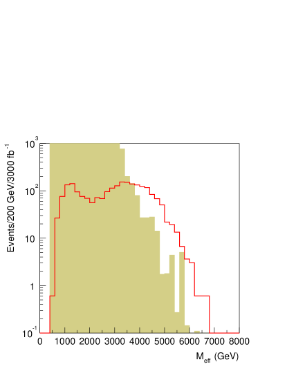
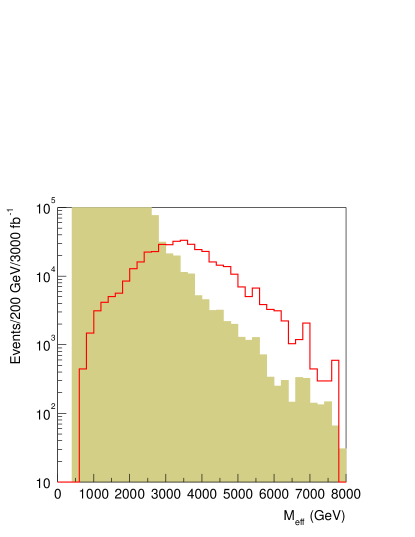
Point K has and gluino and squark masses above . The strong production is dominated by valance squarks, which have the characteristic decays and . The signal can be observed in the inclusive effective mass distribution. Events are selected with hadronic jets and missing , and the following scalar quantity is formed:
where the sum runs over all jets with GeV and and isolated leptons with GeV and . The following further selection was then made: events were selected with at least two jets with , , , and . These cuts help to optimize the signal to background ratio. The distributions in for signal and background are shown in Figure 1. It can be seen that the signal emerges from the background at large values of . The LHC with 3000 of integrated luminosity has a signal of 510 events on a background of 108 for . These rates are sufficiently large so that a discovery could be made with the standard integrated luminosity of 300 . However the limited data samples available will restrict detailed studies.
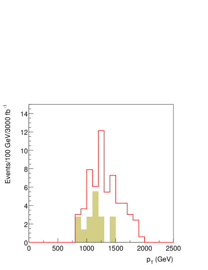
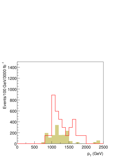
Production of followed by the decay of each squark to gives a dijet signal accompanied by missing . In order to extract this from the standard model background, hard cuts on the jets and are needed. Events were required to have two jets with , , and . The resulting distributions are shown in Figure 2. Only a few events survive at the LHC with 3000 . The transverse momentum of the hardest jet is sensitive to the mass [97]. The mass determination will be limited by the available statistics.
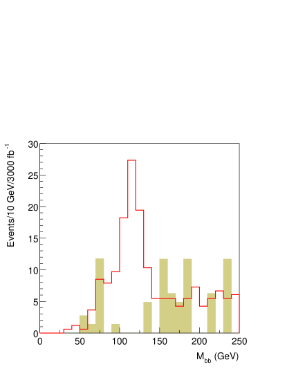
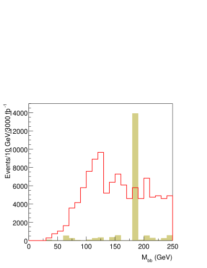
The decay is dominant so we should expect to see Higgs particles in the decay of (). The Higgs signal can be observed as a peak in the mass distributions. In order to do this, it is essential that jets can be tagged with good efficiency and excellent rejection against light quark jets. There is a large background from that must be overcome using topological cuts. Events were selected to have at least three jets with , , , , and . The distributions are shown in Figure 3 assuming the same -tagging performance as for standard luminosity, i.e., that shown in Figure 9-31 of Ref. [97] which corresponds to an efficiency of 60% and a rejection factor against light quark jets of . This tagging performance may be optimistic in the very high luminosity environment. However our event selection is only efficient at SLHC and might be improved. There is much less standard model background at VLHC. However, there is significant SUSY background from which becomes more important at the higher energy. At the VLHC and possibly a the SLHC, it should be possible to extract information on the mass of by combining the Higgs with a jet and probing the decay chain (see e.g. [99]).
3 Point M
Point M has squark and gluino masses around 3.5 TeV and is beyond the reach of the standard LHC. Only 375 SUSY events of all types are produced for at LHC, mainly valence squarks () and gauginos (). The VLHC cross section is a factor of 200 larger. About half of the SLHC SUSY events are from electro weak gaugino pair production mostly and . The dominant decays of these are and . Rates are so small that no signal close to the Standard Model backgrounds could be found for the SLHC.
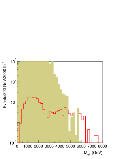
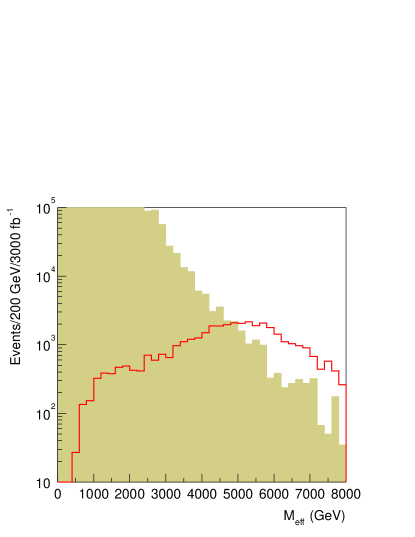
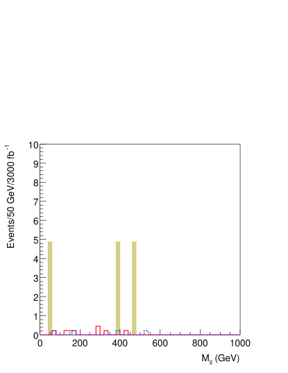
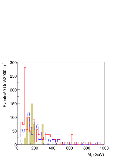
The effective mass distributions for Point M at SLHC and VLHC are shown in Figure 4 using the same cuts as for Point K. As expected, the SLHC signal is very marginal: there are only 20 signal events with 10 background events for and . Several attempts to optimize the cuts did not give any improvement. Requiring a lepton, a hadronic , or a tagged jet did not help. We are forced to conclude that it is unlikely that a signal of any type could be observed. The VLHC signal is clearly visible and could be further optimized.
The dilepton rates are shown in Fig 5. Events are selected that have and two isolated leptons with and the mass distribution of the dilepton pair is shown. As expected, nothing is visible at SLHC. The distribution at VLHC is dominated by two independent decays (e.g. ), so that and rates are almost identical except for the peak in the former which arises mainly from .
On the basis of this preliminary, study it seems unlikely that Point M can be detected at even with . Higher energy would be required.
4 Point H
Point H is able to accommodate very heavy sparticles without overclosing the universe as the destruction rate for the is enhanced by coannihilation with a stau. This implies a very small splitting between the and the . In this particular case, , so it must decay by second order weak processes, , giving it a long lifetime. The dominant SUSY rates arise from the strong production of valance squarks, with and . The staus which are produced from cascade decays of these squarks, then exit the detector with a signal similar to a “heavy muon”.
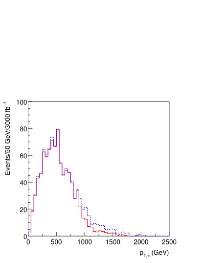
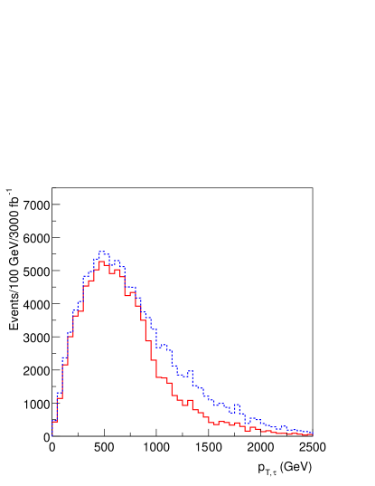
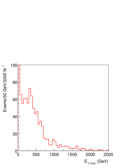
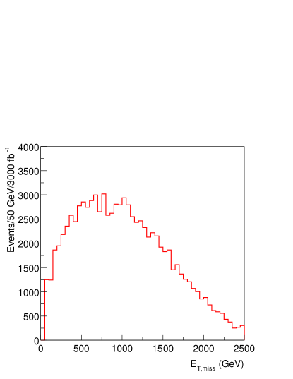
The spectrum of these quasi-stable for is shown in Figure 6. The ATLAS muon system [97] has a time resolution of about 0.7 ns for time of flight over a cylinder of radius 10 m and half-length 20 m. The spectrum with a time delay is also shown. Notice that this signal could be observed at the LHC with . Triggering on a slow may be a problem since the time-window for the trigger chambers is limited. However, the in SUSY events as measured by the calorimeter is quite large as shown in Figure 7. It probably is possible to trigger just on jets plus , the distribution for which is shown in Figure 7. The mass of the stable stau can be measured by exploiting the time of flight measurements in the muon measurement system. Studies of such quasi stable particles at somewhat smaller masses carried out at the ATLAS detector showed a mass resolution of approximately 3% given sufficient statistics (see Section 20.3.4.2 of Ref [97]). A precision of this order should be achievable with 3000 at either the LHC or VLHC. One can then build on the stable stau to reconstruct the decay chain using techniques similar to those used for the GMSB studies [97, 100]. This is not pursued here.
The stable signature is somewhat exceptional so we explore other signatures that do not require it and would be present if the stau decayed inside the detector. For such high masses the strong production is mainly of and . Events are selected with hadronic jets and missing and the effective mass formed as in the case of Point K. To optimize this signature, events were further selected with at least two jets with , , , and . The distributions after these cuts for the SLHC and the VLHC are shown in Fig 8.
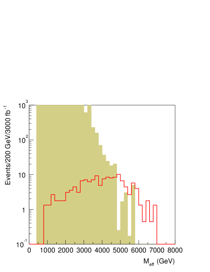
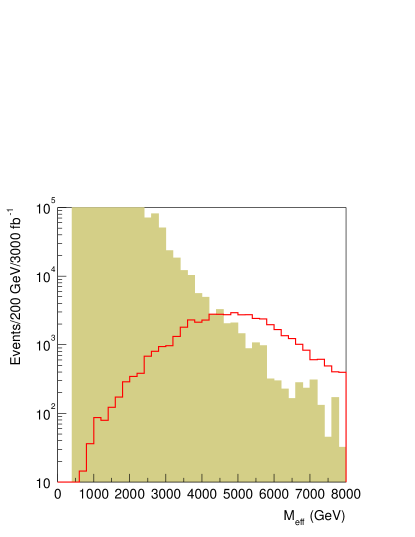
Note that at the SLHC the number of events in the region where is very small. Given the uncertainties in the modeling of the standard model backgrounds via the shower Monte Carlo, it is not possible to claim that the SLHC could see a signal using this global variable. The VLHC should have no difficulty as there are several thousand events for TeV.
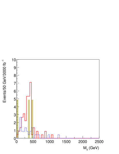
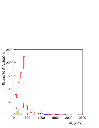
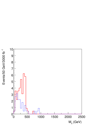
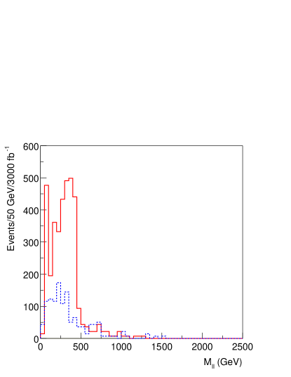
Dileptons arise from the cascade , The dilepton mass distributions should have a kinematic endpoint corresponding to this decay. Figure 9 shows the distribution for same flavor and different flavor lepton pairs. Events were required to have and and to have two isolated opposite sign leptons with GeV and . The structure at the VLHC is clear; the edge comes mainly from , which has a branching ratio of 15% per flavor. This gives an endpoint at
consistent with the observed endpoint in Figure 9. Of course this plot does not distinguish and . In the case of the upgraded LHC, the signal may be observable, but it should be noted that the background is uncertain as only three generated events passed the cuts.
If the stable stau is used then the situation improves considerably. The dilepton mass for events containing a with a time delay is shown in Figure 10. Since , the standard model background is expected to be negligible. The SLHC signal is improved and a measurement should be possible. The acceptance for VLHC is somewhat worse than the inclusive sample, but having the correlation of the dileptons with the should be useful.
The VLHC gives a gain of in statistics over the LHC for the same luminosity at this point, which is at the limit of observability at the LHC. If the VLHC luminosity were substantially lower, the improvement provided by it would be rather marginal. The cross section increases by another factor of at .
5 Conclusions
We have surveyed the signals at hadron colliders for the SUGRA models proposed by [77] concentrating on the cases where the sparticle masses are very large. While the masses of the sparticles at Point K are such that SUSY would be discovered at the baseline LHC, the event rates are small and detailed SUSY studies will not be possible. The reach of the LHC would be improved by higher luminosity where the extraction of specific final states will become possible. The cross section at a VLHC is approximately times larger than that at LHC. This leads to a substantial gain, but it is important to emphasize that this gain requires luminosity at least as large as that ultimately reached by the LHC and detectors capable of exploiting it. Point H has a special feature in that the stau is quasi-stable. This feature would enable a signal to be extracted at SLHC. If the tau mass were raised slightly so that its lifetime were short, then only the VLHC could observe it. The masses in the case of Point M are so large that the VLHC would be required for discovery. Point F has a gluino mass of order 2 TeV and should be observable at the LHC exploiting the production of gluinos followed by the decays to and hence to leptons.
The Points A, B, C, D, G, I, and L which are much less fine tuned have similar phenomenology to the “Point 5” or “Point 6” analysis of [97] in that lepton structure from the decay and/or is present. In most cases decay is also allowed, so that a more complicated dilepton mass spectrum is observable. This should enable the extraction of in addition (for an example see Fig 20-53 of [97]). Points A, D and L have higher squark/gluino masses and will require more integrated luminosity. Nevertheless one can have confidence that the baseline LHC will make many measurements in all of these cases.
6 Acknowledgments
This work was supported in part by the Director, Office of Energy Research, Office of High Energy and Nuclear Physics of the U.S. Department of Energy under Contracts DE–AC03–76SF00098 and DE-AC02-98CH10886. Accordingly, the U.S. Government retains a nonexclusive, royalty-free license to publish or reproduce the published form of this contribution, or allow others to do so, for U.S. Government purposes.
Part VI SUSY with Heavy Scalars at LHC
I. Hinchliffe and F.E. Paige
1 Introduction
SUSY models may give new contributions to flavor changing neutral currents, violation, etc., through loops involving squarks and sleptons. These effects are reduced if the scalars are heavy. The “inverted hierarchy” [101] and “focus point” [102] scenarios provide examples of ways in which heavy scalars could be accommodated naturally.
This note examines the LHC signatures for a minimal SUGRA model with
The gaugino masses are similar to those considered previously, e.g.,
Most of the scalars have masses around ; the light Higgs mass is .
The SUSY production cross section at the LHC is dominated by gluino pairs. The two largest branching ratios are
However, decays into both charginos and all four neutralinos with all allowed combinations of quarks are significant. This leads to many complex signatures.
ISAJET 7.51 was used to generate events for the signal and for all the Standard Model (SM) backgrounds. The detector response to these events was simulated using a parameterized simulation with parameters appropriate to the ATLAS detector. Jets were found using a simple cone algorithm with . Lepton identification efficiency and and jet tagging and misidentification were included with parameterized efficiencies and backgrounds based on full simulation of ATLAS. A micro-DST was saved and subsequently analyzed using Root as a framework. The statistics for the signal correspond to approximately . The statistics for the largest SM background samples correspond to a much smaller luminosity but are sufficient to show that the Standard Model backgrounds are small after cuts.
2 Effective Mass Distribution
An inclusive signature based on multiple jets plus missing energy was useful at many of the SUSY points considered previously and remains so here. Since the jet multiplicity is higher here, the effective mass was defined to include all jets and leptons, not just the four hardest jets:
Events were selected to have
-
•
At least six jets with ;
-
•
;
-
•
Transverse sphericity ;
-
•
.
The resulting distribution for signal and background is shown in Figure 1. In contrast to many previous cases, the signal emerges from the SM background well past its peak, but nevertheless the ratio is large for large enough . Thus, discovery of a deviation from the SM is easy, although not quite so easy as in earlier cases.
This signal can be improved by requiring at least one jet. A tagging probability of 70% was chosen, and the corresponding light jet rejection was taken from full simulation results for ATLAS. This distribution is also shown in Figure 1. As expected, the ratio is improved with only a small loss of signal.
3 Top Reconstruction
Given the large branching ratios for , it is natural to try to reconstruct hadronic top decays. If everything decays hadronically, the jet multiplicity from each gluino is 6 for and 8 for , giving a total of 12 to 16 jets without any gluon radiation. This produces a severe combinatorial background; lepton-based signatures are considerably easier. Work on top reconstruction is continuing. A more sophisticated jet algorithm might work better for these complex events.
4 Signature
The three-body decay has a kinematic endpoint at . Events satisfying the cuts given in Section 2 were required to have two OS,SF leptons with and . The reconstruction efficiency was assumed to be 90% for both and . Figure 2 shows the resulting and mass distributions. Any contribution from two independent decays should cancel in the difference of these. This difference shows both a continuum with an endpoint at the expected place and a peak coming from decays of heavy gauginos.
The largest single source of is ; while the largest sources of heavy gauginos are and . Thus one expects a large fraction of dileptons to be accompanied by a . Figure 2 also shows the subtracted distribution without and with at least one tag.
5 Signature
Two independent leptonic decays of the same gluino, e.g., with and , gives an OS dilepton signature. Since the is a Majorana fermion, any contribution from leptonic decays involving both gluinos will cancel in the combination . (Equal acceptance for and is assumed here. In reality one would have to correct for acceptance; this correction can be checked using data.) The resulting distribution using the cuts described above is shown in Figure 3.
While the dilepton distribution should have a true kinematic endpoint corresponding to the maximum possible mass from gluino decay, this is not useful because many particles are unobservable (, ) or not included (jets). The largest contributions to this channel should come from with and . Three samples of events with (the typical range for the gluino ) and with one of the three decay chains forced were generated. The same analysis was applied except that the required number of jets was reduced from 6 to 3. The mass distributions for the three possibilities are shown in Figure 4. All three are qualitatively similar to that shown in Figure 3. The shapes are somewhat different and presumably could be distinguished with sufficient statistics after a detailed analysis. This has not yet been attempted.
The sign-subtracted pair was next combined with each of the three hardest jets (with ) in the event. The distribution of the minimum of the three masses is shown in Figure 5. The distribution in the case that the jet giving the minimum is tagged as a is also shown in the Figure. If one of the jets is from the same gluino as the dilepton pair, then this distribution should have a kinematic endpoint related to the gluino mass. The choice of three jets is a compromise between including the right jet and including too many. The expected shape from a single gluino was again determined using the sample; this is also shown in Figure 5. A similar analysis combining the with two jets found too much combinatorial background.
If one of the leptons is from , then the smallest mass should be less than the kinematic limit for this decay, . This minimum mass is plotted in Figure 6 and has the expected shape. However, a rather small fraction of the jets so selected are tagged as ’s, while the tagging efficiency is about 60%.
6 Signature
If both gluinos decay via with , the signature is four hard jets plus two leptons. Requiring the leptons to be the same sign causes the loss of half of the signal but greatly reduces the SM background. Events were selected to have
-
•
Four jets with , the first with ;
-
•
;
-
•
;
-
•
;
-
•
At least 2 leptons;
-
•
Less than 2 tagged jets.
The two hardest leptons were required to be the same sign. For each of the three possible ways of pairing the jets, the larger of the dijet masses was taken, so the minimum of the three masses should be less than the dijet endpoint for gluino decay, . The distributions for all three and for the minimum are shown in Figure 7. The expected distribution obtained by forcing the decays and is shown in Figure 8. The endpoint has the expected value. However, the sample is not very pure: Figure 9 shows that there are other contributions. Harder cuts on extra jets did not help significantly to improve the purity.
7 Signature from
The decays have branching ratios of and respectively at this point; has a branching ratio of . The pair was combined with any jet with not tagged as a . Figure 10 shows the resulting mass distributions for the peak and for the continuum. The distribution should have an endpoint at that can be calculated in terms of the masses involved. The continuum is more complicated since the dilepton mass also has a distribution.
8 Signature
Direct production of gauginos is only a factor of smaller than production at this point. Events were selected to have three leptons with . A jet veto of was imposed. The OS,SF dilepton mass distribution is shown in Figure 11. The dilepton endpoint is known from Figure 2. Requiring an OS,SF pair below this endpoint gives the distribution in the same figure. Clearly the SM background is still comparable to the signal; it would be worse if the width in SM events were properly taken into account. Also, the effect of pileup on the jet veto has not been included. Thus this channel does not seem very promising.
9 Acknowledgments
This work was supported in part by the Director, Office of Energy Research, Office of High Energy and Nuclear Physics of the U.S. Department of Energy under Contracts DE–AC03–76SF00098 and DE-AC02-98CH10886. Accordingly, the U.S. Government retains a nonexclusive, royalty-free license to publish or reproduce the published form of this contribution, or allow others to do so, for U.S. Government purposes.
Part VII Inclusive study of MSSM in CMS
S. Abdullin,
A. Albert,
F. Charles
1 Aim
The MSSM is a good candidate for the new Physics expected at the TeV scale. Experiments at both LEP [103] and Tevatron [104] have been looking for evidence of SUSY, but for the moment no signal has been observed. The results of the searches give limits on sparticle masses. Some indirect measurements like the branching ratio, the anomalous muon magnetic moment g-2 [77, 105], dark matter searches [106] or the Z width also provide constraints on SUSY parameter values. But all these results still leave a large MSSM parameter space unexplored.
The goal of this study is to evaluate the ability of the CMS detector [107] to observe signals of supersymmetry in a large domain of MSSM parameter values. The mSUGRA [108, 81] (minimal SUper GRAvity) model, with its only five free parameters (, , , and ) is very popular and has been the subject of many studies up to now. A study of mSUGRA, performed in a similar way [109] to the work presented here, concludes that for both low and high values of , and for both positive and negative , the mass reach for gluinos and squarks is up to to TeV for .
Two reasons motivate us to extend the mSUGRA study to a less constrained model, the “phenomenological” MSSM (pMSSM). On the one hand, mSUGRA is a rather constrained model, very specific and not illustrative of the variety of all possible supersymmetric models. On the other hand, contrary to mSUGRA, the pMSSM has no fixed hierarchy of masses. In this case, some extreme mass hierarchies could show a significantly different kinematical behavior than in the case of mSUGRA, which could prevent the discovery of supersymmetry even for relatively low values of the sparticle masses. Moreover, in the case of pMSSM we have various types of cascades which produce many types of final states, with similar signatures, but not the same types of particles. For example, are we going to be able to observe supersymmetry with a final state containing multiple jets; taus instead of muons and electrons; and jets produced by c quarks instead of b quarks? The type of particles produced is really important in order to discover supersymmetry in CMS and to identify the SUSY scenario at work.
In this pMSSM framework, we are going to show that supersymmetry could be discovered over a large scale of masses in the versus plane. Next we show that there are ways to estimate the values of the MSSM parameters using kinematical quantities measured by the CMS detector and event rates. An advantage of this approach is its model independence – the only dependence comes from the hierarchy of masses [110]. Finally, we estimate the statistical uncertainties due to this method of extraction of the MSSM parameter values.
2 Theoretical framework
2.1 MSSM
Supersymmetry (SUSY) is a symmetry between fermions and bosons. Some of the motivation for SUSY has been reviewed in the Introduction. The MSSM [108, 81] is the Supersymmetric extension of the Standard Model which introduces the minimal number of new particles (only one per SM particle and 4 additional Higgs bosons) and no new couplings. The MSSM contains 124 independent parameters, including the 19 ones of the Standard Model.
2.1.1 pMSSM (phenomenological MSSM)
Some phenomenological constraints allow to reduce the number of MSSM free parameters:
-
•
no new sources of CP violation,
-
•
no Flavor Changing Neutral Current effects,
-
•
universality of the first two generations.
These three constraints leave only 19 free parameters :
-
•
: ratio of the vacuum expectation values of the two Higgs doublets fields,
-
•
: mass of the pseudoscalar Higgs boson,
-
•
: SUSY preserving Higgs mass parameter,
-
•
, , : bino, wino and gluino mass parameters,
-
•
,, , : unified first and second generation sfermion masses,
-
•
, , , , : third generation sfermion masses,
-
•
, , : third generation trilinear couplings.
2.1.2 A restricted pMSSM
The model used in our study is a pMSSM, but with a further reduction in the number of free parameters. It is an intermediate model between mSUGRA and the pMSSM, relaxing the constraints of mSUGRA but still more constrained than the pMSSM. Reference [81] gives some examples of such models, taking into account more constraints than pMSSM. We take into account, respectively, the mass unification of squarks and sleptons (universality of the three generations of sparticles) assuming that the mixing is not too large for the third generation. We also consider the unification of trilinear coupling . This leads to 9 free parameters: , , , , , , , , . This constrained model allows us to perform simpler simulation, while keeping the diversity of signatures of MSSM events.
2.2 Examples of signal events
2.2.1 An example of MSSM cascade
Figure 1 shows an MSSM event of the type , with 5 jets including 2 b quark jets and 3 leptons including 2 ’s in the final state. The 2 neutralinos produce missing transverse energy .
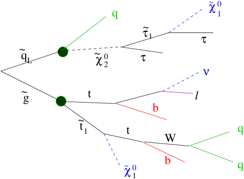
2.2.2 A more detailed mSUGRA example
An mSUGRA event of the type is shown in figure 2(a), while figure 2(b) shows the corresponding event display in CMS obtained from GEANT [111] for this event. We used the following parameter values:
GeV, GeV, , , .
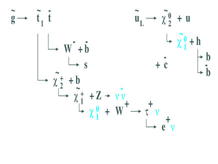
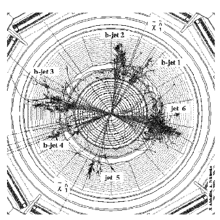
The final state is made of 6 jets including 4 b-quark jets, and 2 neutralinos which produce .
3 Simulation procedure
3.1 Signal production
We use a model with 9 parameters, which make up a hyperspace in 9 dimensions. To simplify the analysis we use a discretization of the parameter values. The choice of the number of values for each parameter depends on the parameter sensitivity. We used a grid for squark and gluino masses with 9 values evenly spaced between 600 and 3000 GeV, because the event characteristics at LHC depend primarily on these two masses. On the other hand, many observables are not very strongly dependent on the parameter . We thus use only two values, to distinguish the behavior at large and small values of this parameter. The values selected for each parameter in this analysis are the following:
-
•
: GeV
-
•
: GeV
-
•
: GeV
-
•
: GeV
-
•
: GeV
-
•
: GeV
-
•
: GeV
-
•
: GeV
-
•
:
We end up with a total of 140000 different sets of parameter values. For each set, we generate 1000 events, a compromise between the limits imposed by the handling of the data flow and sufficiently small statistical errors. The theoretical and experimental constraints make it possible to reduce the number of combinations to a total of .
These imposed constraints are the following:
-
•
constraint on the Higgs mass GeV,
-
•
lightest chargino mass GeV,
-
•
lightest neutralino mass GeV,
-
•
the lightest neutralino is the LSP.
Signal events were generated using the ISAJET program [98]. The CMS detector response was obtained from the fast Monte-Carlo code (non-Geant) CMSJET 4.51 [112]. Characteristics of CMSJET software are given in figure 3.
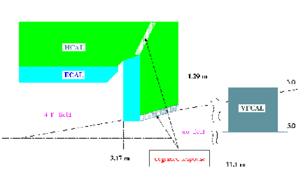
3.2 Background production
The background production to this , SUSY search was estimated using Standard Model events leading to similar signatures as the MSSM events. The background was produced using PYTHIA [113]. We consider here SUSY signals with the following event characteristics:
-
•
production from 0 to n isolated leptons (electrons or muons),
-
•
a large value for the average missing transverse energy ( GeV),
-
•
more than 2 jets with large transverse energy ( GeV).
Therefore we must consider as potential Standard Model backgrounds all processes with large rest masses which yield large transverse missing energy, producing energetic jets, and possible isolated leptons. Thus the backgrounds we consider are the following: . We also consider events with several high energy jets, including heavy flavors (b and c). The missing transverse energy in this type of event originates either from semi-leptonic b,c decay or from imperfections and fluctuations in the response of the detector which may fake missing transverse energy. Some of the background mechanisms are shown in figure 4. The primary contributions to the background after cuts is at large values of the transverse momentum of the produced particles in the 2-body final state. To obtain sufficient statistics, we generate events independently for several intervals of (see table 1). A total of two hundred million events have been generated.
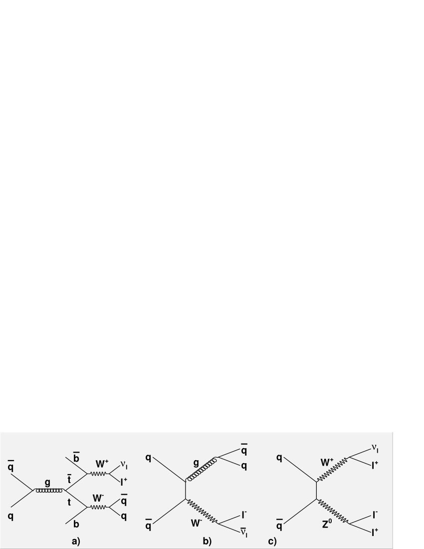
| processes | interval (GeV) | (pb) | Nev generated | % of needed for |
| total |
The QCD event sample generated for low is tiny compared to the required one but fortunately, there is correlation between and the maximal produced value, so one does not expect high values of for low . To be confident in the simulation, we apply some preliminary cuts during the generation:
-
•
GeV limit, below which the QCD jet background become dominant;
-
•
at least 2 jets with GeV in .
The isolation of the leptons is given by the following requirement
-
•
muon with GeV within the muon acceptance or electron with GeV within ;
-
•
no charged particles with GeV in a cone of around the direction of the lepton;
-
•
in a cone ring around the lepton impact point has to be less than 10% of the lepton transverse energy.
3.2.1 Pile-up
We also take into account event pile-up, i.e. 25 inelastic events on average per bunch crossing with a Poisson distribution. The two upper graphs in figure 5 illustrate the ratio between the lepton isolation efficiency with and without pileup, as a function of pseudorapidity, and transverse momentum (the definition of lepton isolation is given in [112]). The efficiency is reduced to 85% due to the multiplicity of particles produced in each bunch crossing. In the two lower plots giving the event missing transverse energy, and the scalar sum of the event transverse energy, the solid curves are without pile-up and the dashed ones with pile-up. Pile-up does not make a very significant difference for total missing transverse energy, but increases the total transverse energy.

3.3 Different selection criteria
To distinguish signal from background, we are led to apply kinematical cuts on the observables we extract from the CMS detector.
Table 2 gives all the different values we use for the selection. This yields approximately 10000 combinations of cuts to optimize signal to background ratio.
3.4 Signal significance estimator
We make a systematic search for all sets of parameters and thus define limits of discovery through calculations of the significance of the signals. The definition of the significance we use is the following one:
| (1) |
where is the number of signal events and the number of background events. A significance exceeding 5 indicates that the corresponding set of MSSM parameter values is experimentally accessible. In order to optimize the significance, we used some cuts which are listed in the Table 2.
| parameter | different cut values |
|---|---|
| Number of jets | 2, 3, 4, 5, 6, 7, 8, 9, 10 jets |
| (with a minimal transverse energy of 40 GeV) | |
| Transverse momentum of the highest energy jet | 40, 150, 300, 400, 500, 600, 700, 800, 900, 1000 GeV |
| Transverse momentum of the second highest energy jet | 40, 80, 200, 300, 400, 500 GeV |
| Missing transverse momentum | 200, 300, 400, 500, 600, 700, 800, |
| 900, 1000, 1100, 1200, 1300, 1400 GeV | |
| Total transverse momentum | 700, 900, 1100, 1300, 1500, 1700, 1900, 2100, |
| 2300, 2500, 2700, 2900, 3100, 3300, 3500 GeV | |
| Angle between the missing transverse | 0, 20 degrees |
| momentum and the momentum of the isolated lepton |
| before cuts | after cuts | |
| number of signal events | 6152 | 431 |
| number of background events | 240 | 124 |
| significance | 0.397 | 38.614 |
| before cuts | after cuts | |
| number of signal events | 6121 | 355 |
| number of background events | 240 | 112 |
| significance | 0.395 | 33,5 |
To show the importance of cuts to separate the signal from the background, tables 3 and 4 give examples of the number of events for signal and background, before and after cuts. We notice the very important effect of the cuts, the number of background events decreasing from to , i.e. by a factor roughly equal to , and the significance increasing by a factor 100.
4 Analysis
4.1 Calculation of significance
4.1.1 Illustration of the analysis for some specific parameter values
Figure 6(a) gives distributions of signal (in black) and backgrounds (in gray) for some kinematical quantities before any cuts are applied; the signal is not easily distinguishable from the background at this stage, as the cross section is too much smaller. But quantities such as and have a very different shape, thus cutting on these variables would greatly enhance the signal to background ratio.
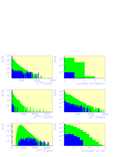
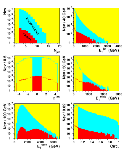
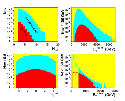
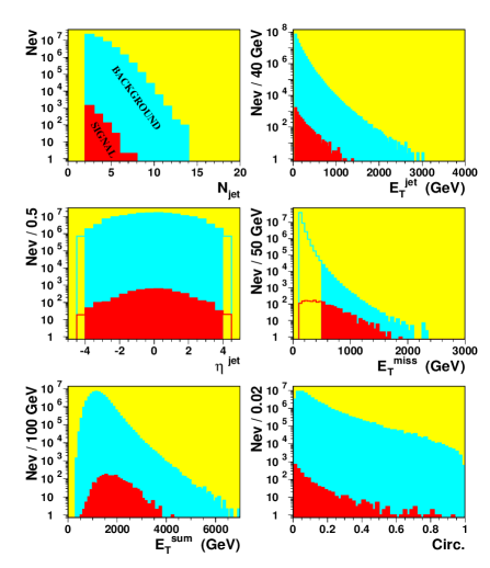
The specific example shown in figure 6(a) corresponds to the following values of MSSM parameters:
| (2) |
The cross section for this set of parameters is , and the significance after applying all cuts is equal to 33.
4.1.2 Example with either very broad or very narrow hierarchy of masses
We have investigated in some detail one of the major points of difference between mSUGRA and pMSSM, namely the non fixed hierarchy of masses in case of pMSSM. In the first example (figure 6(b)), with a very broad mass spectrum, the masses of neutralinos are chosen to be much lower than the masses of squarks, gluinos and sleptons. Sparticles production is therefore dominated by neutralinos and charginos. The specific parameter values are the following:
| (3) |
The cross section for this set of parameters is pb and despite the abundance of neutralinos and the low production rate of gluinos and squarks, one is still able to obtain after appropriate cuts (discussed in the following section) a significance equal to .
As a second example (figure 6(c)) we chose a case where the masses of the neutralinos, gluinos, squarks and sleptons are comparable. The specific parameter values are the following:
| (4) |
SUSY production now mostly proceeds via gluinos and squarks with a cross section pb and a significance equal to after selection cuts.
For the third example (figure 6(d)) the parameter values are the following:
| (5) |
The masses of the neutralinos, gluinos, squarks and sleptons are similar again but heavier than in the previous example. The main sparticle production proceeds still via gluinos and squarks, with, in this case, a cross section pb and a significance equal to after cuts are applied.
Even for the sets of parameter values which would seem difficult (either very similar masses or on the contrary very broad span of masses), applying cuts allows to obtain good results. However, in the case of a small spread of sparticle masses, the discovery limit is about 1.5 TeV instead of 2.5 TeV as obtained with the usual mSUGRA-type mass hierarchies.
4.1.3 Discovery limits
We now generalize this study to determine a limit of discovery for the MSSM. For each MSSM point, we are looking for the set of cuts which gives the maximum value for the significance. With these collected values of the maximal significance, we can draw the discovery limits (estimated as the isocurve of a significance equal to 5). The significances are calculated for an integrated luminosity corresponding to one year of LHC at high luminosity. Our first result is the isocurve of significance equal to 5, given in the plane , which are the two most important parameters. The 7 other parameters have the same fixed value for all the MSSM points of the plane.
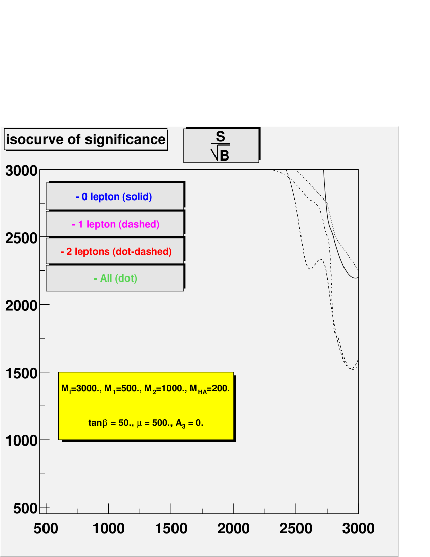
One example of such a result is given by Figure 7 with the following values of the other parameters:
| (6) |
Four isocurves are given in this figure, corresponding to a specific event topology selection according to the number of isolated leptons produced. The curves labelled “0 lepton”, “1 lepton”, “2 leptons” correspond to a calculation of significance using only events with respectively , , lepton(s). The curves labelled “all” use all events to calculate the significance. For each point and each type of lepton selection, we manage to find the set of cuts which gives the largest significance.
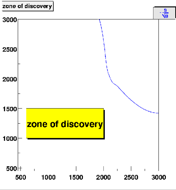
We can now try to compile all these results in one characteristic limit. We could first combine our results in a conservative fashion, establishing the region in the plane in which any set of the orthogonal parameters will be accessible by the CMS detector. In other words, for each point in the plane above the reach curve there exist at least one set of the 7 other parameter which has a significance under 5. Figure 8 shows this pessimistic mass reach in the plane. In terms of statistics, there are a total of 2,962 combinations (out of the original 35,000 combinations of parameters) which don’t pass the cut on significance (). We have also found a single point under the curve which does not pass the significance cut:
| (7) |
This particular point exhibits a narrow hierarchy of masses just like in the previous example, and provides a lower limit of discovery. In a typical configuration we have a discovery limit of about 2.5 TeV. This exact reach in parameter space depends on the magnitude of the background cross section within the kinematical cuts. Here, we assume that the PYTHIA cross section are correct. This is clearly invalid, as higher order QCD corrections to , W+jets, Z+jets are not incorporated. This is an aspect of systematic uncertainties to be addressed in a later study.
4.2 From kinematical observables to MSSM parameters
4.2.1 Choice of observables
In a second exercise, we reverse the problem and try to see whether on the basis of event kinematical variables and event rates it would be possible to determine the MSSM parameter values. A total of 11 observables are used to separate the different sets of MSSM parameter values.
-
•
average number of leptons per event ,
-
•
average number of jets per event ,
-
•
mean value of jet momenta ,
-
•
mean value of lepton momenta ,
-
•
mean value of missing transverse energy ,
-
•
number of events ,
-
•
number of events with 0,1,2 or 3 leptons , , , ,
-
•
mean value of total transverse energy .
These observables are characteristic of the measurement to be done with the CMS detector, and correspond to signatures of MSSM events. In particular, there are correlations between these observables and the MSSM parameters.
Figure 9 illustrates some of these correlations between observables and pMSSM parameters, more specifically, between , , , and the parameter .

The values of the other parameters are:
| (8) |
It can be seen that the value of all these kinematical quantities decreases with increasing . This shows that these observables are sensitive to the value of . We have obtained the same behavior with the other pMSSM parameters, which is an argument to use pMSSM instead of mSUGRA.
4.2.2 Separation of parameters
After optimizing the cuts to achieve maximal significance, we extract the values of all observables for signal and background, and we calculate the statistical uncertainties associated with each observable; the uncertainties are equal to the ratio of the standard deviation of the distribution and the number of events, thus :
-
•
for number of events (for example the number of events with 0 leptons);
-
•
in general and for mean value ( like ) with the root mean square.
In this way we take into account the uncertainties on the averages derived from the small number of 1000 events generated for each MSSM point. Can these values of the observables be linked to the values of the pMSSM parameters? In other words, are we able to distinguish two different sets of MSSM parameter values using only the values of the observables for each set? If this discrimination is possible, we associate each set of parameter values with the corresponding values of kinematical quantities, and also we use interpolation when we turn to the continuous case. Discrimination is carried out in the following way: one MSSM point is considered distinguishable from another one when the difference between values of at least one of the observables for the two points is greater than 5 standard deviations of the considered observable , calculated for the point we take as reference, i.e. if, for example, where is the number of jets for the reference point, is the number of jets for another points and is the statistical uncertainty on the average number of jets of the reference point. By calculating, for each MSSM point, the difference between the MSSM reference point and any other point for each observable and by expressing these variations in terms of the value of respective uncertainties calculated for the reference point, we can discriminate between them.

Figure 10 shows an example of discrimination for the following values of parameters:
| (9) |
By applying successively a cut at 5 standard deviations on the following observables: average number of leptons, of jets, missing transverse energy and total transverse energy, we manage to separate the reference point from all the other ones. This method works for all MSSM points ( the number of cuts needed for the separation varies from point to point).
4.2.3 Evaluation of the statistical uncertainties
We showed in the previous section that there is a possibility to distinguish one set of parameter values from the others. We are now going to estimate the statistical uncertainties for each MSSM parameter value. We estimate these uncertainties using the uncertainties calculated for each observable. For that, we consider one set of MSSM parameter values defined as the reference point. Then for any chosen parameter, we measure the number of standard deviations for each observable between the reference point and the MSSM point having the same parameter values except for the one in question. The value of this parameter has to be different by one unit on the grid of values. For example, if we want to obtain the statistical uncertainties on the parameter for fixed values of the other parameters, we consider the point which has the same values for the other parameters and the next higher value for in the grid of parameters and then we calculate
| (10) |
where is the missing transverse energy at the point we want to calculate the resolution, the missing transverse energy at the other point and the statistical uncertainty estimate for . We assumed that
| (11) |
where is the statistical uncertainty we want to estimate. We could also take another observable or a linear combination of observables to calculate the uncertainties.
In the following two tables, we have used as the observable for the calculation of the resolution.
| parameter | value | ||
|---|---|---|---|
| M() (GeV) | |||
| M1 (GeV) | |||
| M2 (GeV) | |||
| M() (GeV) | |||
| M() (GeV) | |||
| A (GeV) | |||
| (GeV) | |||
| A3 |
| parameter | value | ||
|---|---|---|---|
| M() (GeV) | |||
| M1 (GeV) | |||
| M2 (GeV) | |||
| M() (GeV) | |||
| M() (GeV) | |||
| A (GeV) | |||
| (GeV) | |||
| A3 |

Tables 5 and 6 show some examples of resolution obtained by this method. These values are small since this is only the statistical error. The resolution should degrade after including systematic errors. Table 5 shows the calculation of statistical resolution for medium squark and gluino masses, where statistics are large. Table 6 shows a similar calculation for large masses for squarks and gluinos, where statistics are low and the uncertainties are thus much more important.
Figure 11 shows an example of resolution in the plane versus for the following reference point:
| (12) |
We have, for this point, a resolution of about 5 to 10 GeV (using the number of events with 0 leptons, , as the discriminator).
5 Conclusion
We demonstrated the possibility to discover a phenomenological MSSM using an inclusive study in the MSSM parameters space. Once we have discovered SUSY, using the kinematical observables for parameter determination proved to be an efficient method. Statistical uncertainties obtained are relatively small ( GeV for squark and gluino masses). We could note, at the end of our study, that there was little difference between mSUGRA and the pMSSM. The discovery limit is to a large extent determined by the total cross section (and is around 2.7 TeV at CMS). The only difference appears for some points having a specific mass hierarchy. As an example, in the case of a compact hierarchy of masses, the limit we expect is about 1.5 TeV.
Part VIII Establishing a No-Lose Theorem for NMSSM
Higgs Boson Discovery at the LHC
U. Ellwanger, J.F. Gunion, C. Hugonie
1 Introduction
Supersymmetric extensions of the standard model generally predict relatively light Higgs bosons. One of the most important tasks of the LHC is the search for Higgs bosons [79, 114, 96]. An important milestone in understanding the potential of the LHC was the demonstration that at least one Higgs boson of the minimal supersymmetric standard model (MSSM) would be detectable at the level throughout all of the MSSM parameter space so long as top squark masses do not exceed 1.5 to 2 TeV and so long as large branching fractions to decay channels containing supersymmetric particles are not substantial.
In [115], we studied, subject to these same and a few other simplifying restrictions, the detectability of Higgs bosons in the next-to-minimal supersymmetric standard model (NMSSM). This short note presents the most relevant procedures and conclusions of [115]. In the NMSSM, one Higgs singlet superfield, , is added to the MSSM in order to render unnecessary the bilinear superpotential term by replacing it with , where the vacuum expectation value of the scalar component of , , results in an effective bilinear Higgs mixing with . The detectability of the NMSSM Higgs bosons was first considered in a contribution to Snowmass 96 [116]. The result, using the experimentally established modes and sensitivities available at the time, was that substantial regions in the parameter space of the NMSSM were found where none of the Higgs bosons would have been observable either at LEP2 or at the LHC even with an integrated luminosity of (two detectors with each).
Since then, progress has been made both on the theoretical and the experimental sides. On the theoretical side, the dominant two-loop corrections to the effective potential of the model have been computed [117, 118]. These lead to a modest decrease in the mass of the lightest Higgs scalar, holding fixed the stop sector parameters. Inclusion of the two-loop corrections thus increases somewhat the part of the NMSSM parameter space excluded by LEP2 (and accessible at the Tevatron) [118], but is of less relevance for the LHC. On the experimental side the expected statistical significances have been improved since 1996 [79, 114, 96]. Most notably, associated production with (originally discussed in [119]), which in the SM context is particularly sensitive to GeV, has been added by ATLAS and CMS to the list of Higgs boson detection modes [79, 114, 96, 120, 121, 122, 123]. Analysis of this mode was recently extended [124] to , which, though not relevant in the SM case due to the decline in the branching ratio as the mode increases, is highly relevant for points in our searches for which the mode is suppressed in comparison to the SM prediction. In addition, techniques have been proposed [125, 126, 127, 128, 129, 130] for isolating signals for fusion to a light Higgs boson which decays to or .
It turns out that adding in just the process renders the no-Higgs-discovery parameter choices described and plotted in [116], including the “black point” described in detail there, visible [131]. In [115], we searched for any remaining parameter choices for which no Higgs boson would produce a signal. In this search, we performed a scan over nearly all of the parameter space of the model, the only parameter choices not included being those for which there is sensitivity to the highly model-dependent decays of Higgs bosons to other Higgs bosons and/or superparticles. The outcome is that, for an integrated luminosity of at the LHC, there are still regions in the parameter space with expected statistical significance (computed as for a given mode) for all Higgs detection modes so far studied in detail by ATLAS and CMS, i.e. including the mode but not the -fusion modes. On the other hand, the expected statistical significance for at least one of these detection modes is always above at , and the statistical significance obtained by combining (using the naive Gaussian procedure) all the non--fusion modes is at least . However, we find that all such cases are quite observable (at ) in one of the -fusion modes (using theoretically estimated statistical significances for these modes). For all points in the scan of parameter space, statistical significances obtained by combining all modes, including -fusion modes, are always . Thus, NMSSM Higgs discovery by just one detector with is essentially guaranteed for those portions of parameter space for which Higgs decays to other Higgs bosons or supersymmetric particles are kinematically forbidden. This represents substantial progress towards guaranteeing LHC discovery of at least one of the NMSSM Higgs bosons.
In order to clarify the nature of the most difficult points in those portions of parameter space considered, we present, in sect. 4, examples of particularly difficult bench mark points for the Higgs sector of the NMSSM. Apart from the “bare” parameters of the model, we give the masses and couplings of all Higgs scalars, their production rates and branching ratios to various channels (relative to the SM Higgs) and details of the statistical significances predicted for each Higgs boson in each channel. The latter will allow an assessment of exactly what level of improvement in statistical significance will be required in the various different detection modes in order to render marginal modes visible. Of course, our estimates of the expected statistical significances are often somewhat crude (e.g. their dependence on the accumulated integrated luminosity). We believe that our procedures always err in the conservative direction, leading to statistical significances that might be a bit small. Thus, the LHC procedures for isolating Higgs boson signals could provide even more robust signals for NMSSM Higgs boson detection than we estimate here.
The detection modes, which serve for the searches for standard model or MSSM Higgs bosons, include (using the notation , for CP-even, CP-odd Higgs bosons, respectively):
1) ;
2) associated or production with in the final state;
3) associated production with ;
4) or associated production with ;
5) 4 leptons;
6) ;
7) LEP2 and ;
8) ;
9) ,
where 8) and 9) are those analyzed at the theoretical level in [125, 126, 127, 128, 129, 130] and included in the NMSSM analysis for the first time in this paper. The above detection modes do not employ the possibly important decay channels i) , ii) , iii) , iv) , v) , vi) , vii) , viii) and ix) . The decay modes i)-vii) give high multiplicity final states and deserve a dedicated study [132], while the existing analyses of the final state signatures are not very detailed. Further, when kinematically allowed, the signal would be easily observed according to existing analyzes. Thus, in this paper we restrict our scan over NMSSM parameter space to those parameters for which none of these decays are present. In addition, we take the constraints of LEP2 [via the mode 7)] into account, and only accept points for which discovery at LEP2 would not have been possible [133, 134].
The Higgs sector of the NMSSM consists of 3 scalars, denoted with , 2 pseudo-scalars, denoted with , and a charged Higgs pair, denoted . Mixing of the neutral doublet fields with the gauge singlet fields in the scalar and in the pseudo-scalar sector can be strong. The scalar mixing can lead to a simultaneous suppression of the couplings of all the to gauge bosons, and hence to a suppression of many of the detection modes above. (Of course, the have no tree-level couplings to gauge boson pairs and the one-loop couplings are too small to yield useful event rates.) The couplings of the Higgs bosons to t- or b-quarks can be amplified, reduced or even change sign with respect to the standard model couplings. Hence negative interferences can occur among the (loop-) diagrams contributing to and , leading again to suppressions of the above detection modes. A complete simultaneous annulation of all detection modes is not possible, but simultaneous reduction of all detection modes is possible and it is for such parameter choices that NMSSM Higgs boson discovery is most difficult.
In the next section, we define the class of models we are going to consider, and the way we perform the scan over the corresponding parameter space. In section 3 we describe our computations of the expected statistical significances of the detection modes 1) – 9) above. In section 4, we present six particularly difficult bench mark points (in table 1) and details regarding their statistical significances in channels 1)-9) in table 2, with a summary of overall statistical significances in table 3. Using these tables, we give a discussion of the properties of these points.
| Point Number | 1 | 2 | 3 | 4 | 5 | 6 |
|---|---|---|---|---|---|---|
| Bare Parameters | ||||||
| 0.0340 | 0.0450 | 0.0230 | 0.0230 | 0.1330 | 0.0230 | |
| 0.0198 | 0.0248 | 0.0129 | 0.0069 | 0.1459 | 0.0114 | |
| 6.00 | 5.25 | -5.5 | 5.75 | -8 | -6 | |
| 140 | -110 | 115 | -235 | 100 | 150 | |
| -35 | 25 | -95 | 40 | -135 | -100 | |
| -150 | 70 | -90 | 80 | -75 | -110 | |
| Scalar Masses and Couplings | ||||||
| (GeV) | 115 | 100 | 103 | 113 | 114 | 112 |
| -0.66 | 0.32 | -0.34 | 0.67 | -0.87 | -0.71 | |
| -0.65 | 0.30 | -0.31 | 0.65 | -0.81 | -0.66 | |
| -1.07 | 0.66 | -1.27 | 1.16 | -4.50 | -2.40 | |
| gg Production Rate | 0.39 | 0.08 | 0.08 | 0.39 | 0.56 | 0.36 |
| 0.43 | 0.26 | 0.09 | 0.38 | 0.05 | 0.11 | |
| 1.12 | 1.08 | 1.10 | 1.12 | 1.18 | 1.15 | |
| 0.42 | 0.25 | 0.08 | 0.37 | 0.04 | 0.10 | |
| (GeV) | 125 | 114 | 114 | 126 | 144 | 122 |
| -0.74 | -0.83 | 0.79 | -0.73 | 0.46 | 0.59 | |
| -0.72 | -0.74 | 0.70 | -0.71 | 0.57 | 0.54 | |
| -1.49 | -3.28 | 3.46 | -1.47 | -6.66 | 2.24 | |
| gg Production Rate | 0.46 | 0.44 | 0.40 | 0.45 | 1.18 | 0.23 |
| 0.33 | 0.08 | 0.07 | 0.34 | 0.01 | 0.10 | |
| 1.30 | 1.18 | 1.18 | 1.32 | 3.06 | 1.31 | |
| 0.32 | 0.08 | 0.06 | 0.33 | 0.01 | 0.09 | |
| (GeV) | 205 | 153 | 148 | 201 | 202 | 155 |
| -0.14 | -0.46 | -0.51 | -0.15 | 0.18 | -0.39 | |
| -0.30 | -0.63 | -0.67 | -0.32 | 0.17 | -0.55 | |
| 5.80 | 4.17 | 4.20 | 5.53 | 0.68 | 5.12 | |
| gg Production Rate | 0.31 | 0.84 | 0.95 | 0.33 | 0.02 | 0.80 |
| 0.13 | 0.05 | 0.05 | 0.15 | 0.98 | 0.03 | |
| 308.66 | 5.83 | 3.92 | 274.41 | 13.97 | 8.12 | |
| 0.18 | 0.07 | 0.06 | 0.21 | 0.96 | 0.05 | |
| Pseudo-Scalar Masses and Couplings | ||||||
| (GeV) | 191 | 112 | 130 | 130 | 113 | 145 |
| 0.03 | -0.03 | -0.10 | -0.01 | -0.10 | -0.16 | |
| 1.16 | -0.83 | -2.95 | -0.19 | -6.55 | -5.77 | |
| gg Production Rate | 0.00 | 0.00 | 0.03 | 0.00 | 0.31 | 0.08 |
| (GeV) | 206 | 141 | 137 | 198 | 174 | 158 |
| 0.16 | 0.19 | -0.15 | 0.17 | -0.07 | -0.05 | |
| 5.89 | 5.18 | -4.64 | 5.75 | -4.59 | -1.65 | |
| gg Production Rate | 0.02 | 0.07 | 0.06 | 0.02 | 0.03 | 0.00 |
| Charged Higgs Mass | ||||||
| (GeV) | 221 | 162 | 157 | 213 | 157 | 167 |
| Point | 1 | 2 | 3 | 4 | 5 | 6 |
|---|---|---|---|---|---|---|
| Channel | Higgs boson | |||||
| 3.74 | 0.35 | 0.13 | 3.18 | 0.62 | 0.83 | |
| 4.37 | 0.59 | 0.22 | 3.92 | 0.85 | 1.22 | |
| 2.79 | 0.85 | 0.85 | 3.03 | 4.83 | 3.30 | |
| 0.08 | 0.07 | 0.76 | 0.09 | 4.52 | 0.40 | |
| 0.83 | 0.00 | 0.00 | 0.64 | 0.12 | 0.16 | |
| 1.10 | 0.09 | 0.03 | 0.90 | 0.16 | 0.22 | |
| 0.00 | 3.37 | 3.40 | 3.29 | 0.00 | 4.79 | |
| 9.29 | 1.22 | 1.59 | 8.93 | 16.78 | 10.08 | |
| 2.39 | 0.00 | 0.00 | 1.74 | 0.41 | 0.49 | |
| 6.54 | 1.09 | 1.17 | 5.99 | 6.69 | 3.65 | |
| 6.54 | 3.55 | 3.59 | 6.84 | 6.69 | 6.02 | |
| 11.61 | 1.64 | 1.97 | 10.89 | 18.07 | 10.73 | |
| 11.61 | 3.75 | 3.93 | 11.38 | 18.07 | 11.75 | |
| Channel | Higgs boson | |||||
| 3.69 | 0.83 | 0.61 | 3.62 | 0.22 | 0.55 | |
| 4.01 | 1.25 | 0.92 | 3.93 | 0.05 | 0.74 | |
| 2.49 | 3.95 | 3.58 | 2.30 | 0.99 | 1.77 | |
| 0.16 | 2.76 | 2.93 | 0.16 | 3.62 | 2.99 | |
| 1.84 | 0.16 | 0.11 | 1.94 | 0.56 | 0.20 | |
| 1.44 | 0.22 | 0.16 | 1.46 | 0.38 | 0.18 | |
| 0.00 | 0.00 | 3.31 | 0.00 | 0.00 | 0.00 | |
| 15.39 | 15.17 | 13.46 | 15.05 | 7.41 | 9.89 | |
| 5.79 | 0.63 | 0.44 | 6.05 | 0.19 | 0.82 | |
| 6.44 | 5.05 | 4.76 | 6.31 | 3.82 | 3.61 | |
| 6.44 | 5.05 | 5.80 | 6.31 | 3.82 | 3.61 | |
| 17.65 | 16.00 | 14.28 | 17.40 | 8.34 | 10.56 | |
| 17.65 | 16.00 | 14.66 | 17.40 | 8.34 | 10.56 | |
| Channel | Higgs boson | |||||
| 0.00 | 0.59 | 0.66 | 0.01 | 0.00 | 0.32 | |
| 0.00 | 0.21 | 0.25 | 0.00 | 0.00 | 0.08 | |
| 0.00 | 0.00 | 1.13 | 0.00 | 0.00 | 0.00 | |
| 3.79 | 3.43 | 3.62 | 3.56 | 1.55 | 4.86 | |
| 3.65 | 2.51 | 2.07 | 4.46 | 1.54 | 1.66 | |
| 0.80 | 2.13 | 1.52 | 1.17 | 0.38 | 1.55 | |
| 0.00 | 0.00 | 0.00 | 0.00 | 0.00 | 0.00 | |
| 0.00 | 0.00 | 9.06 | 0.00 | 0.00 | 0.00 | |
| 0.00 | 0.77 | 0.79 | 0.00 | 0.00 | 0.43 | |
| 5.32 | 4.80 | 4.64 | 5.83 | 4.76 | 5.37 | |
| 5.32 | 4.80 | 4.64 | 5.83 | 4.76 | 5.37 | |
| 5.32 | 4.86 | 10.21 | 5.83 | 4.76 | 5.39 | |
| 5.32 | 4.86 | 10.21 | 5.83 | 4.76 | 5.39 | |
| Point Number | 1 | 2 | 3 | 4 | 5 | 6 |
| Best non- fusion | 4.37 () | 3.95 () | 3.62 () | 4.46 () | 4.83 () | 4.86 () |
| Best fusion | 15.39 () | 15.17 () | 13.46 () | 15.05 () | 16.78 () | 10.08 () |
| Best combined w.o. -fusion modes | 6.54 () | 5.05 () | 4.76 () | 6.31 () | 6.69 () | 5.37 () |
| Best combined with -fusion modes | 17.65 () | 16.00 () | 14.28 () | 17.40 () | 18.07 () | 10.73 () |
2 NMSSM Parameters and Scanning Procedure
In this paper, we consider the simplest version of the NMSSM [135, 136, 137, 138, 139, 140, 141, 142, 143, 144, 145, 146, 147, 148], where the term in the superpotential of the MSSM is replaced by (we use the notation for the superfield and for its scalar component field)
| (1) |
so that the superpotential is scale invariant. We make no assumption on “universal” soft terms. Hence, the five soft supersymmetry breaking terms
| (2) |
are considered as independent. The masses and/or couplings of sparticles are assumed to be such that their contributions to the loop diagrams inducing Higgs production by gluon fusion and Higgs decay into are negligible. In the stop sector, which appears in the radiative corrections to the Higgs potential, we chose the soft masses TeV, and varied the stop mixing parameter
| (3) |
As in the MSSM, the value – so called maximal mixing – maximizes the radiative corrections to the Higgs masses, and we found that it leads to the most challenging points in the parameter space of the NMSSM.
Assuming that the Higgs sector is CP conserving, the independent parameters of the model are thus: and . For purposes of scanning and analysis, it is more convenient to eliminate , and in favor of , and through the three minimization equations of the Higgs potential (including the dominant 1- and 2-loop corrections [118]) and to scan over the six independent parameters
| (4) |
We adopt the convention , in which can have either sign. The absence of Landau singularities for and below the GUT scale ( GeV) imposes upper bounds on these couplings at the weak scale, which depend on the value of and hence of [135, 136, 137, 138, 139]. Using GeV, one finds and for intermediate values of .
For each point in the parameter space, we diagonalize the scalar and pseudo-scalar mass matrices and compute the scalar, pseudo-scalar and charged Higgs masses and couplings taking into account the dominant 1- and 2-loop radiative corrections [118]. We then demand that the Higgs scalars satisfy the LEP2 constraints on the production mode (taken from [133], fig. 10), which gives a lower bound on as a function of the reduced coupling. We also impose LEP2 constraints on associated production (from [134], fig. 6), yielding a lower bound on as a function of the reduced coupling.
In order to render the above-mentioned processes i) – ix) kinematically impossible, we require the following inequalities among the masses:
In addition we require GeV; otherwise a light chargino would have been detected at LEP2. (The precise lower bound on depends somewhat on and the precise experimental lower bound on the chargino mass; however, our subsequent results do not depend on the precise choice of the lower bound on .) We further note that for the most challenging parameter space points that we shall shortly discuss, is already sufficient to guarantee that the NMSSM Higgs bosons cannot decay to chargino pairs so long as the SU(2) soft-SUSY-breaking parameter is also large. In fact, in order to avoid significant corrections to and couplings coming from chargino loops it is easiest to take (or vice versa). This is because the coupling is suppressed if the is either pure higgsino or pure gaugino. Since the parts of parameter space that are challenging with regard to Higgs detection typically have , the validity of our assumptions requires that be large and that the chargino be essentially pure higgsino.
Using a very rough sampling, we determined, as expected from previous work [116], that it is only for moderate values of that signals might possibly occur. From this sampling, we determined the most difficult parameter space regions and further refined our scan to the following:
-
•
(both signs) in steps of 0.25;
-
•
, using 20 points;
-
•
, using 20 points;
-
•
(both signs), in steps of 5 GeV;
-
•
, with opposite in sign to , using steps of 5 GeV;
-
•
, with opposite in sign to , using steps of 5 GeV.
For those points sampled in this final scan which satisfy all the constraints detailed earlier, we compute the expected statistical significances for the processes 1) to 9) listed in section 1, as described in the next section. As a rough guide, from the points detailed in the above list, we find about that pass all constraints and have (for ) in each of the individual discovery modes 1) – 7). We shall tabulate a number of representative points taken from this final set in section 4.
3 Expected Statistical Significances
¿From the known couplings of the NMSSM Higgs scalars to gauge bosons and fermions it is straightforward to compute their production rates in gluon-gluon fusion and various associated production processes, as well as their partial widths into , gauge bosons and fermions, either relative to a standard model Higgs scalar or relative to the MSSM and/or . This allows us to apply “NMSSM corrections” to the processes 1) – 9) above.
These NMSSM corrections are computed in terms of the following ratios. For the scalar Higgs bosons, is the ratio of the coupling of the to vector bosons as compared to that of a SM Higgs boson (the coupling ratios for and are the same), and , are the corresponding ratios of the couplings to top and bottom quarks (one has ). Note that we always have , but and can be larger, smaller or even differ in sign with respect to the standard model. For the CP-odd Higgs bosons, is not relevant since there is no tree-level coupling of the to the states; and are defined as the ratio of the couplings for and , respectively, relative to SM-like strength.
We emphasize that our procedure implicitly includes QCD corrections to the Higgs production processes at precisely the same level as the experimental collaborations. First, the ATLAS and CMS collaborations employed Monte Carlo programs such as ISAJET [98] and PYTHIA [113] in obtaining results for the (MS)SM. These programs include many QCD corrections to Higgs production in a leading-log sense. This is the best that can currently be done to implement QCD corrections in the context of experimental cuts and neural-net analyses. Clearly the more exact NNLO results for many of the relevant processes will slowly be implemented in the Monte Carlo programs and increased precision for Higgs discovery expectations will result. Since our goal is to obtain NMSSM results that are completely analogous to the currently available (MS)SM results, we have proceeded by simply rescaling the available (MS)SM experimental analyses. In doing the rescaling of the Higgs branching ratios we have included all relevant higher-order QCD corrections [149] using an adapted version of the FORTRAN code HDECAY [150]. Details regarding our rescaling procedures can be found in [115]. Using the rescaling procedures, for each point in the parameter space of the NMSSM we obtain the statistical significances predicted for an integrated luminosity of for each of the detection modes 1) – 9). In order to obtain the statistical significances for the various detection modes at , we multiply the statistical significances by in the cases 1), 2), 3), 5) and 6), but only by a factor of in the cases 4), 8) and 9). That such a factor is appropriate for mode 4), see, for example, fig. 19-62 in [79]. Use of this same factor for modes 8) and 9) is simply a conservative guess.
4 Difficult Points
As stated in the introduction we still find “black spots” in the parameter space of the NMSSM, where the expected statistical significances for all Higgs detection modes 1) – 7) are below at . The reasons for this phenomenon have been described above; see also the corresponding discussion in [116]. However, after including the modes 8) and 9), the points that provide the worst 1) – 6) statistical significances typically yield robust signals in one or the other of the -fusion modes 8) and 9).
In order to render the corresponding suppression mechanisms of the detection modes reproducible, we present the detailed properties of several difficult points in the parameter space in table 1. The notation is as follows: The bare parameters are as in eq. (2.5), with , and fixed implicitly by the minimization conditions. (As noted earlier, with the convention , in the NMSSM, the sign of can no longer be defined to be positive.) For the reasons discussed below eq. (3) we chose in the stop sector TeV and for all of the points (1 – 6). We have also fixed GeV. For both scalar and pseudoscalar Higgs bosons, “gg Production Rate” denotes the ratio of the gluon-gluon production rate with respect to that obtained if , keeping the Higgs mass fixed. For scalar , this is the same as the ratio of the production rate relative to that predicted for a SM Higgs boson of the same mass. For the scalar , denotes the ratio of the branching ratio with respect to that of a SM Higgs boson with the same mass. (A verification of the reduced gluon-gluon production rates or branching ratios would sometimes require the knowledge of the couplings to higher precision than given, for convenience, in table 1.) Also given for the scalar are the ratios and of the and branching ratios relative to the SM prediction (as noted above, one has ).
In table 2, we tabulate the statistical significances for the in all the channels 1) – 9); production of the CP-odd turns out to be relevant only when they add to the signals in process 4). Also note that, all these problematical points are such that , so that followed by would have been kinematically forbidden at the highest LEP2 energy. Hence, for LEP2 mode 7) we only give the statistical significance for . Also tabulated in table 2 are four statistical significances obtained by combining various channels. This combination is done in the Gaussian approximation:
where runs over the channels being combined. We give results for the following combinations:
-
a) obtained by combining LHC channels 1) – 6);
-
b) obtained by combining LHC channels 1) – 6) and LEP2;
-
c) obtained by combining LHC channels 1) – 6) with the -fusion channels 8) and 9);
-
d) obtained by combining all LHC channels and LEP2, i.e. by combining all channels 1) – 9).
In those cases where there is no LEP2 signal, a)=b) and c)=d). In addition, in our point selection we have required a mass difference of at least 10 GeV between scalar Higgses, so that they yield well separated signals and no statistical significance combination of two different scalar Higgses is needed. All parameter choices for which Higgs boson masses differ by less than 10 GeV yield stronger signals than the cases retained. (The increased net signal strength of overlapping Higgs signals in those channels with limited mass resolution arises as a result of .)
As summarized in table 3, all of the tabulated “bench mark points” have statistical significances below for all of the detection modes 1) – 6) at and 7) at LEP2. In more detail, as tabulated in table 2 and summarized in table 3, the best signals in the modes 1) – 6) for the points #1 – #6 at the LHC are:
-
•
point #1, 4.37 for mode 2) and ;
-
•
point #2, 3.95 for mode 3) and ;
-
•
point #3, 3.62 for mode 4) and ;
-
•
point #4, 4.46 for mode 5) and ;
-
•
point #5, 4.83 for mode 3) and ;
-
•
point #6, 4.86 for mode 4) and ;
Further, for point #3, the combined statistical significance of modes 1) – 6) (also tabulated in table 3) would still be below for any one , although (as is likely to be relevant by combining ATLAS and CMS data once each detector has accumulated ) for at least one of the . However, for all these “difficult” points the -fusion modes 8) and/or 9) provide (according to theoretical estimates) a decent (sometimes very strong) signal.
The points #1 – #4 differ as to which of the modes 1) – 6) and which yields the largest statistical significance should the -fusion mode 8) not provide as strong a signal as suggested by the theoretical estimates. To render these points observable without the -fusion mode 8) would require improvements of all detection modes 2) – 5).
As in [116], we find that difficult points in the parameter space generally have . This is the region of for which the signals are still not very much enhanced but yet the and signals have been suppressed somewhat. In a few cases, however, difficulties also arise for as large as 8, as shown in the case of point #5. Also as in [116], the most difficult points are those in which the masses of the and are relatively close in magnitude, typically clustered in a interval above . Such clustering maximizes the mixing among the different Higgs bosons and thereby minimizes the significance of the discovery channels for any one Higgs boson. In particular, it is for strong mixing among the that the statistical significance for discovery modes based on a large coupling for any one are most easily suppressed.
Finally, for point #6, we have minimized the statistical significances for the -fusion modes over the parameter space, while keeping the statistical significances of modes 1) – 6) below 5. One can see that it still gives a strong signal in mode 8). [Smaller for mode 8) would have been possible if we had allowed stronger signals in modes 1) – 6), in particular had we allowed smaller mass separation, , between the two lightest Higgs bosons.] In addition, for point #6 GeV and the coupling of is sufficiently large that it would have yielded a signal at LEP2. Had we taken a top quark mass slightly larger, GeV, we would have found a very similar point with a mass of GeV, which could have been responsible for the excess observed at LEP2 [151, 152, 153, 154].
5 Discussion and Conclusions
In this paper, we have addressed the question of whether or not it would be possible to fail to discover any of the Higgs bosons of the NMSSM using combined LEP2 and LHC data, possibly resulting in the erroneous conclusion that Higgs bosons with masses below 200 GeV have been excluded. We have demonstrated that, assuming that the decay channels i) – ix) are either kinematically disallowed or render a Higgs boson observable, this is unlikely (at the level) to happen. Certainly, there are points in NMSSM parameter space for which the statistical significances for the individual detection modes 1) – 6) (i.e. those analyzed in detail by ATLAS and CMS) are all well below for integrated luminosity of . However, by combining several of the modes 1) – 6) and data from both ATLAS and CMS, a signal can be achieved based just on modes 1) – 6). Further, we have found that throughout all of the NMSSM parameter space (scanned subject to the earlier listed restrictions) for which such weak signals in modes 1) – 6) are predicted, the theoretical estimates for the -fusion modes indicate that an easily detected signal should be present. Thus, our conclusion is that for all of the parameter space of the NMSSM compatible with reasonable boundary conditions for the parameters at the GUT scale (with, of course, non-universal soft terms in general) and such that Higgs pair and SUSY pair decays of the Higgs bosons are kinematically forbidden, at least one of the NMSSM Higgs bosons will be detected at the LHC. This is a big improvement over the results from the earlier Snowmass 1996 study which was somewhat negative without the inclusion of the mode 3), and the -fusion modes 8) and 9).
It is amusing to note that all of our bench mark points for which Higgs discovery is most difficult at the LHC include a Higgs scalar with mass close to 115 GeV (with, however, reduced couplings to the boson), which could be responsible for the excess observed at LEP2 [151, 152, 153, 154].
Another important point that appears from our analysis is the fact that the full of integrated luminosity (per detector) is needed in order to have robust NMSSM Higgs discovery in the portion of parameter space considered here. Of course, as in the MSSM, it is very possible that only one of the CP-even NMSSM Higgs bosons might be detected at the LHC but that, as studied by Kamoshita et al. in [140, 141, 142, 143, 144, 145, 146, 147, 148], the observation of all the CP-even Higgs bosons of the NMSSM would be possible at the LC by virtue of all having some non-negligible level of coupling and not having very high masses. Even at the LC, the CP-odd Higgs bosons might escape discovery, although this would not be the case for the parameter choices that we have found which make LHC discovery of even one NMSSM Higgs bosons most challenging. This is because, for such parameters, the are relatively light and could be readily seen at the LC in the processes , and , assuming an integrated LC luminosity of and energy [155].
This study makes clear the importance of continuing to expand the sensitivity of existing modes and continuing to develop new modes for Higgs detection at the LHC in order not to have to wait for construction of a linear collider for detection of at least one of the SUSY Higgs bosons. In particular, study of modes i) – ix) and SUSY pair channels should all be pushed. The problematical points that we have emphasized here are unlikely to be substantially influenced by or SUSY decays since all the Higgs masses are below so that decays will be kinematically highly suppressed (one of the top quarks would have to be virtual) and SUSY pair decays are quite unlikely to be significant given LEP2 limits on the masses of SUSY particles. However, by allowing Higgs (in particular, pseudoscalar) masses such that one or more of the channels i)-vii) are kinematically allowed we have found points for which discovery in modes 1)-9) will not be possible [132]. Thus, a full “no-lose” theorem for NMSSM Higgs boson discovery at the LHC will require exploring additional discovery modes sensitive to those portions of parameter space for which Higgs decays to other Higgs bosons are important, and might necessitate combining results from both the ATLAS and CMS detectors and/or accumulating more integrated luminosity.
6 Acknowledgments
We wish to acknowledge helpful discussions with M. Sapinski and D. Zeppenfeld. C.H. would like to thank the late theory group of the Rutherford Appleton Laboratory and the Theoretical Physics Department of Oxford, where part of this work was achieved, for their kind hospitality. This work was supported in part by the U.S. Department of Energy.
Part IX Effects of Supersymmetric Phases on Higgs Production
in Association with Squark Pairs
in the Minimal Supersymmetric Standard Model
A. Dedes, S. Moretti
It has recently been shown [156, 157, 158, 159, 160, 161, 162] that, if CP-violating effects are manifestly inserted into the MSSM Lagrangian, by allowing the Higgsino mass term, , and the trilinear couplings, ¶¶¶For simplicity, we assume at the electroweak (EW) scale, i.e., , where and refer to all flavors of up- and down-type (s)quarks., to be complex, thereby introducing two independent CP-violating phases [163, 164], and , such that and , then the strength of the Higgs couplings to (s)particles can drastically be modified, inducing sizable effects, e.g., in the dominant production mode of neutral Higgs bosons at the LHC, i.e., (where and ), through the squark-squark-Higgs vertices involving stops and sbottoms. These effects are a consequence of large values attained by and/or consistent with cancellations taking place in the SUSY contributions to the Electric Dipole Moments (EDMs) of neutron and electron [165, 166, 167, 168].
These same interactions also affect the associated production of Higgs bosons with third generation squark pairs. Since this process is expected to be accessible at the LHC, see Refs. [169, 170, 171, 172, 173, 174, 175], we investigate here some aspects of its phenomenology in the presence of complex parameters in the MSSM Lagrangian. Schematically, the production mechanism is the following:
| (1) |
where , and , in all possible combinations, as appropriate in the MSSM. Notice that in such processes the existence of CP-violating effects in the SUSY Lagrangian would immediately be manifest from the detection of three particle final states involving a pseudoscalar Higgs boson and two identical squarks. In fact, if , even in presence of mixing between the third-generation squarks, the couplings, with and , are identically zero [171]. Depending on the relative value of the final state masses in (1), , and , the production of Higgs particles can be regarded as taking place either via a (anti)squark decay or via a Higgs-strahlung.
We work in the theoretical framework provided by the ‘complex’ MSSM, the latter including explicitly the two CP-violating phases, and , and assuming universality of the soft gaugino masses only at the Grand Unification (GUT) scale. We define its fundamental parameters without making any assumptions about the structure of the SUSY breaking dynamics at the Planck scale, whether driven by Supergravity (SUGRA), gauge/anomaly mediated (GMSB/AMSB) or proceeding via other mechanisms as we treat the MSSM as a low-energy effective theory. Among the possible setups of the MSSM parameter space compatible at one-loop with the EDM data, we choose here the one presented in Table 1, in terms of , , (the mass of the pseudoscalar Higgs state), (the ratio of the vacuum expectation values of the two Higgs doublet fields), (the soft squark masses of the three squark generations) and (the soft gluino mass). For this choice of MSSM inputs, the derived masses of the scalar are barely consistent with the latest bounds on from LEP2, of about 91 GeV [176] ( is instead set above the Tevatron limit from Run 1, around 140 GeV [177] for our ). This means that our specific parameter point will readily be probed at the LHC, as in correspondence of the inputs given in Table 1 and by varying both and between 0 and , one has that the lightest Higgs mass spans from 91 to 100 GeV and the lightest stop one is between 140 and 240 GeV or so. Notice that the MSSM setup given in Table 1 should be regarded as one possible example of the rich phenomenology that can be induced by the CP-violating phases in the MSSM with a low and squark/Higgs masses small enough to be produced at detectable rates via process (1). In fact, we have found many others but refrained from showing them here for reasons of space.
In the remainder, we will denote the regions of the () plane excluded from Higgs and squark direct searches by a shaded area. In addition, the inputs in Table 1 comply with the constraints deduced from the two-loop Barr-Zee type contributions to the fermionic EDMs [178, 179] (green “” symbols in the following) for most choices of and . Finally, some () points will further be neglected following the requirement of positive definiteness of the squared squark masses: see eqs. (5)–(6) of Ref. [158, 159, 160, 161, 162] (magenta “” symbols in the forthcoming plots). The top-left corner of Fig. 1 shows the phase dependence of and , outside such experimentally excluded areas.
In the course of our discussion, we shall make only one simplification, which will not alter the conclusions of our work. That is, we will neglect one-loop mixing effects among the three neutral Higgs bosons of the MSSM [180, 181, 182, 183, 184, 185], on the ground that for our choice of parameters they turn out to be of the order of a few percent at most (see discussion in Refs. [156, 157, 158, 159, 160, 161, 162]). Indeed, much larger effects will remain unaccounted for, such as the higher-order QCD corrections to the production process (1), which are likely to induce -factors of the order 1.5–2 and whose calculation is presently not available.
| 600 | 2500 | 300 | 1000 | 200 | 2.7 |
We start our numerical analysis by referring to Fig. 1 of Ref. [156, 157], where one can find the contour plots for the minimum values of the modulus of the common trilinear coupling, , above which the mentioned cancellations work at a level which is compatible with the experimental accuracy achieved in both the neutron and electron EDM measurements, i.e., [186] and [187], for the choice of parameters in Table I and as a function of and . These values are those entered in the production vertices of the processes we considered, alongside the two discrete quantities and . As for the Higgs masses, we keep fixed at 200 GeV and derive the values of and at two-loop level (see the discussion in Refs. [156, 157, 158, 159, 160, 161, 162] concerning the residual theoretical error on the latter).
Among the processes of the type (1), much emphasis has been put on the case in which both the squark and Higgs scalar states are the lightest, that is, on the mechanism [169, 170]. In fact, if the typical scale is in the TeV regime, then two concurrent effects take place, that render light Higgs production in association with the lightest scalar top quarks a more favorable Higgs discovery channel than the corresponding SM-like one, [188, 189]. On the one hand, since the mixing angle is proportional to , the squark becomes much lighter than the -quark and all other squarks. On the other hand, by looking at the expression of the vertex (e.g., see eq. (3) of Ref. [169]), for large values, it is clear that its strength can overcome that of the top-Higgs Yukawa coupling entering the SM-like reaction.
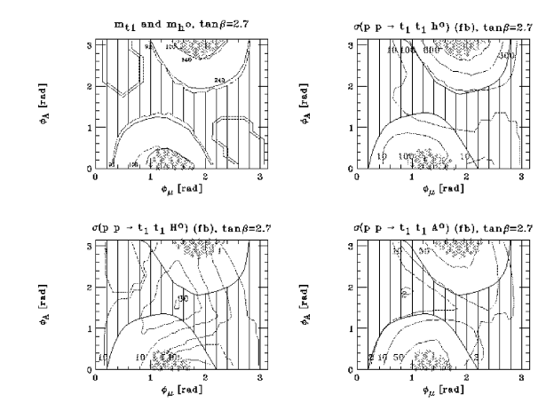
We thus continue our investigation of squark-squark-Higgs production by considering this particular final state. Our choice of in Table I reflects the remark made in Refs. [169, 170] that the production rates are larger at smaller (see, e.g., Fig. 3 of Ref [169]), this being the consequence of the increase of for large values of the latter [158, 159, 160, 161, 162]. (As representative of the low regime, the two values were used in Refs. [169, 170].) As for the spectrum, we are bound to those values guaranteeing the EDM cancellations (again, see Fig. 1 in [156, 157]): that is, between 100 and 700 GeV, depending on and . The top-right corner of Fig. 1 presents the cross sections for as a contour plot over the () plane. We see a strong dependence on the SUSY phases, as the production rates vary over several orders of magnitude. The maximum of the cross section occurs at large values, when is slightly above . This can be understood in the following terms. Here, it is where the lightest stop mass reaches its allowed minimum. However, the fact that does not grow similarly at small values, when is slightly below – the other region of the () plane where is minimal – implies that the vertex too plays an important rôle in determining the actual size of the cross section. The fact that this coupling is maximal where the stop mass is minimal can easily be understood by noticing the dependence of eqs. (5) and (A.53) of Ref. [158, 159, 160, 161, 162] when . Besides, a large value of the coupling combined with a small value of implies that the two-loop contributions of the Barr-Zee type graphs to the EDMs can be sizable, so that it is not surprising to see that larger rates for accumulate towards the correspondingly excluded area. However, in areas not yet removed through the EDM measurements, one can find production rates as large as 800 fb. Finally, notice that – for the choice of parameters in Table I and 100 GeV 700 GeV as in Fig. 1 of [156, 157] – in the ‘phaseless’ limit, i.e., the standard MSSM case, , the yield is several orders of magnitude smaller, indeed well below detection level.
A strong hierarchy exists, , among the neutral Higgs masses, for our setup of the MSSM. This should naturally allow one to disentangle in the experimental samples from events. Furthermore, under the assumption that the lightest scalar quark will promptly be discovered at the LHC from some other source of SUSY events than those in (1), and its mass measured, we believe that final states with two heavy objects of identical mass recoiling against a rather central one with mass (that, again, we assume to be known and reconstructed through and/or decays), should be distinguishable from other channels (), in which or , e.g., in the transverse mass distributions of the visible and decay products.
Even in such circumstances though, and events would still obey a sort of degeneracy in their appearance (especially after accounting for large detector resolutions in reconstructing masses), that could render non-trivial the operation of separating data containing one type from those induced by the other. (Our choice of MSSM parameters, producing , ought to be representative also of such extreme experimental conditions.) Nonetheless, we see that the maxima and minima of and occur in very different regions of the () plane. Moreover, in the allowed areas, the difference between the production rates of the two processes can even be a factor of 10 or more. In other terms, although it could always be possible to attempt the above ‘separation’ on the basis of the different decay patterns of the two Higgs bosons (and/or their topology), this might not be needed after all. In fact, as long as , and have been constrained to some extent through some other measurements, then for some specific values of , a clear excess (i.e., well above the size of the uncertainties induced by unknown higher order QCD effects) of events, with 200 GeV 210 GeV, above the rates, could only be explained if events have indeed been produced.
By comparing the bottom-left to the bottom-right plots in Fig. 1, one realises that this separation can happen over a large portion of the () plane. One should also note the very different shapes of the two contours, such that rates are largest where the ones are smallest. For example, just outside the areas excluded by the EDMs (when or and ), the pseudoscalar Higgs channel can reach the 100 fb level, whereas the scalar Higgs rates are always around 10 fb. For and (or, quite symmetrically, for and ), the two process rates are of the same order, about 10 fb. Finally, in the limit , is about 10 fb and is, of course, zero.
In our numerical simulations, we also have considered the large scenario. However, in this case, once the EDM constraints were taken into account, we have found that both the theoretical plausibility of the MSSM and the phenomenological impact of the CP-violating phases were much reduced. On the one hand, in order to obtain the mentioned cancellations also for , one would need to have the soft squark masses as large as 6 TeV or more and the gluino one TeV, that is, a quite ‘unnatural’ hierarchy in the soft SUSY breaking sector, if one aims to maintain around 300 GeV (so that final states remain within the reach of the LHC energy). On the other hand, for large values, the not yet excluded (by direct searches, two-loop effects in the EDMs and positive definiteness of the squark masses) area of the plane is much smaller (see Fig. 3 of Ref. [158, 159, 160, 161, 162]). (Besides, also mixing effects among neutral Higgs states start becoming relevant for ). Thus, although some sporadic points over the allowed () regions can still be found, these yielding cross sections significantly different from those obtained in the phaseless case, we would conclude that only the region is relevant in the experimental analysis of squark-squark-Higgs production.
To summarise, we have shown that the LHC production rates of the lightest Higgs boson of the MSSM in association with a pair of lightest stop scalars are strongly affected by the presence of complex parameters in the soft sector of the SUSY Lagrangian, even when EDM constraints are taken into account. As a matter of fact, the mechanism has recently been advocated as a new possible discovery mode of the boson, at least for certain combinations of the MSSM parameters, that we have emulated here to some extent. Thus, our results in this case have a twofold meaning. On the one hand, they emphasise that more inputs than those pertaining to a phaseless MSSM could be needed to describe the phenomenology of events (further recall that we have limited ourselves to the case of only two independent phases, and , those associated to the Higgsino mass and the universal trilinear couplings, respectively). On the other hand, they make the point that such a mechanism can be useful in assessing whether or not soft CP-violating phases are present.
In this last respect, however, it would be even more intriguing to detect final states involving the pseudoscalar Higgs boson in place of the lightest scalar one at the LHC. In fact, no matter the actual setup of the MSSM parameters, the detection of a state would unequivocally mean that and/or are finite. In fact, the corresponding interaction is prohibited at tree-level in a MSSM with real masses and couplings in the soft sector and EW effects at the one-loop level are unlikely to yield production rates as large as those shown here: up to 10000 events per year for some phase combinations at high collider luminosity. Further notice that, in our analysis, we deliberately have chosen a small value of , so that mixing effects among the three neutral Higgs states are very small even when the values of and are rather close. Finally, despite this mass degeneracy between the heavy scalar and pseudoscalar Higgs bosons, the relative production rates of and events are very different, both in size and in shape, over most of the () plane, so that the two samples could even be separated experimentally.
Part X Study of the Lepton Flavor Violating Decays of Charged Fermions
in SUSY GUTs
T. Blažek
Neutrino oscillations clearly show that individual lepton flavor is violated in nature. Here we present results of a study of lepton flavor violating decays in a class of SUSY GUT models assuming that the third right-handed neutrino couples equally to the second and third lepton doublets with a large coupling. This corresponds to the neutrino Yukawa matrix (in the left-right basis) of the form
| (1) |
The large 23 entry, responsible for the large atmospheric neutrino mixing angle, induces potentially large lepton flavor violating effects in the low-energy effective theory. The see-saw mechanism yields a physical neutrino with a mass about eV consistent with the SuperKamiokande observation providing the third right-handed neutrino mass is GeV, much greater than the masses of the other two right-handed neutrinos.
We focus on the large tan regime of these models with . The rate of a decay is enhanced by and can be, approximately, rescaled by this factor for lower values of tan. Thus our study provides for the upper estimate of the lepton flavor violating decay rates of charged fermions. In Figure 1a-b we present the results for the branching ratio in a typical model of this class. Besides (1) all other Yukawa matrices are hierarchical with small off-diagonal entries (more details can be found in [191]). The model assumes the Pati-Salam symmetry at the GUT scale GeV but the results in the leptonic sector would be quite similar for models with different unifying gauge group leading to Eq. (1). The two plots were obtained for two different values of the parameter fixed to GeV in plot (a) and GeV in plot (b). is the soft universal scalar mass and is its gaugino analogue, both at . The contour lines in Figure 1a-b should be compared to the experimental upper bound . The allowed region overlaps with the region preferred by the data on the muon , as shown in plots 1c-d. Clearly, this decay rate should be very close to the present limits and thus presents an exciting opportunity to observe lepton flavor violation or to constrain substantially this class of models.
The decays and are much more model dependent since small Yukawa entries are necessarily involved. In the model studied in [191] they are found to be well below the experimental limit. Thus our main result is the correlation between the maximal atmospheric mixing angle and large branching ratio related through the large off-diagonal entry in the Yukawa matrix in (1).
Part XI Interactions of the Goldstino Supermultiplet with Standard Model
Fields
D.S. Gorbunov
1 Goldstino supermultiplet
In any supersymmetric extension of the Standard Model (SM) of particle physics spontaneous supersymmetry breaking occurs due to a non-zero vacuum expectation value of an auxiliary component of some chiral or vector superfield. As a simple case, let us consider a model where
| (1) |
is the only chiral superfield which obtains a non-zero vacuum expectation value for its auxiliary component,
| (2) |
Then is a two-component Goldstone fermion, goldstino, and its superpartners
| (3) |
are respectively a scalar and a pseudoscalar sgoldstino.
In the framework of supergravity becomes the longitudinal component of the gravitino, due to the super-Higgs effect. As a result, the gravitino acquires a mass which in realistic models with a vanishing cosmological constant is completely determined by the supersymmetry breaking parameter :
| (4) |
The sgoldstinos remain massless at tree level and become massive due to corrections from higher order terms in the Kähler potential. If these terms are sufficiently suppressed, the sgoldstinos are light and may appear in particle collisions at high energy colliders. Such pattern emerges in a number of non-minimal supergravity models [192, 193] as well as in gauge mediation models if supersymmetry is broken via a non-trivial superpotential (see, e.g. [194, 195] and references therein). Here we shall consider the sgoldstino masses and as free parameters.
The gravitinos and sgoldstinos interact with the MSSM fields and the corresponding coupling constants are inversely proportional to the supersymmetry breaking parameter . Eq. (4) then implies that the gravitino has to be very light, otherwise the gravitino as well as the sgoldstinos are effectively decoupled from the MSSM fields at the energy scale of the colliders of the near-term future.
2 Effective Lagrangian
The effective Lagrangian for the gravitino is obtained from N=1 supergravity [196], and may be used to calculate scattering processes involving any of the helicity components of the massive gravitino. Meanwhile the energy scale attainable at the present and the nearest future generation of accelerators favors the longitudinal component of gravitino as the most promising to be studied in collision experiments. In this case the longitudinal component of the gravitino, , effectively behaves as a two-component fermion , the goldstino, and the interaction between the goldstino and the other fields is plainly given by the Goldberger–Treiman relation
with being a supercurrent.
In order to obtain the low-energy effective Lagrangian for sgoldstinos one can use the spurion method [197]. It exploits the fact that, by definition, sgoldstinos are scalar components of the very supermultiplet whose auxiliary component acquires a non-zero vacuum expectation value due to supersymmetry breaking. Then one can consider a simple supersymmetric model with non-renormalizable interactions between and the MSSM superfields, which yield the MSSM soft terms when a non-zero is generated. Consequently, the corresponding coupling constants are fixed by the ratios of the soft terms and .
In general, the supersymmetry breaking part of the Lagrangian has the form
| (5) |
where () runs over all scalar (gaugino ) fields. Since supersymmetry is broken spontaneously, Eq. (5) implies the following effective interaction between the MSSM superfields and the goldstino supermultiplet :
where
These terms emerge if the fields from the hidden sector, where supersymmetry breaking occurs, are integrated out. The only remnant of the hidden sector is the goldstino supermultiplet, which may remain light.
Integrating over , and taking into account Eqs. (1), (2) we obtain the soft supersymmetry breaking terms (5) as well as the interactions between the components of the goldstino supermultiplet and the components of the MSSM superfields:
| (6) | |||||
| (7) | |||||
| (8) | |||||
Here we presented only the leading order in terms; the convention for the Levi–Civita tensor is .
Eliminating the auxiliary fields, one obtains the low-energy effective Lagrangian for the interactions between the components of the goldstino supermultiplets and the MSSM fields.
3 Phenomenology of the model
Until now, there is no experimental evidence for a gravitino or sgoldstinos. The study of their phenomenology places bounds on their coupling constants. Note that all sgoldstino coupling constants introduced in the previous sections are completely determined by the MSSM soft terms and the supersymmetry breaking parameter , while the sgoldstino masses and remain arbitrary. Depending on the values of and , the sgoldstinos may show up in different experiments. The phenomenologically interesting models can be separated into four classes:
- •
- •
-
•
Models with flavor violation in the soft trilinear couplings, — sgoldstino interactions then lead to flavor violating processes. In particular, sgoldstinos may contribute to FCNC (mass differences and/or CP-violation in the neutral meson systems) [203, 204], and, if kinematically allowed, sgoldstinos appear in rare decays such as [205], , [202], etc.
-
•
The sgoldstinos are lighter than 1 MeV — these models may be tested in low energy experiments [202], such as reactor experiments, conversion in a magnetic field, etc. Sgoldstinos may also play a very important role in astrophysics and cosmology [206, 207, 208, 202]: they may change the predictions of Big Bang Nucleosynthesis, distort the CMB spectrum, affect SN explosions and the cooling rate of stars, etc.
4 Incorporation into CompHEP
To leading order in and to zero order in the MSSM gauge and Yukawa coupling constants, the interactions between the components of the goldstino supermultiplet and the MSSM fields are derived in Ref. [200]. They correspond to the processes most attractive for collider studies – where only one of these new particles appears in a final state. In this case the light gravitino behaves exactly as a goldstino. For sgoldstinos, as they are R-even, only the sgoldstino-goldstino and sgoldstino-SM fields couplings have been included as the most interesting phenomenologically. All new coupling constants between the components of the goldstino supermultiplet and the MSSM fields are completely determined by the ratios of the soft supersymmetry breaking parameters and . This Lagrangian has been incorporated (see Ref. [200] for details) into the CompHEP software package ∥∥∥The CompHEP package [209] automatically calculates tree-level particle decay rates and cross sections and is aimed to improve the accuracy, to cut down the efforts and to shorten the time usually required for studying high-energy collision processes.. This package may be used in the calculation of any tree-level process with one on-shell gravitino or sgoldstino. The universality of the Lagrangian makes it possible to apply the package in studying the phenomenology of any supersymmetric extension of the Standard Model. Being included into CompHEP, this model should be regarded as an additional option allowed within the framework of the CompHEP/SUSY model. Currently accessible versions of this package operate only with real parameters and coupling constants. Likewise the trilinear soft couplings are assumed to be proportional to the corresponding Yukawa couplings, . The sgoldstino Lagrangian transformed in accordance with these rules reads
| (9) | |||||
| (10) | |||||
5 Remarks
It is worth noting that the independent direct measurement of the MSSM soft supersymmetry breaking terms and the gravitino or/and sgoldstino couplings offers a unique possibility to estimate the supersymmetry breaking scale .
The sgoldstino couplings to superpartners become relevant for models with heavy sgoldstinos, where the sgoldstinos also decay to SM superpartners. In the spurion approach the corresponding coupling constants are not completely determined by the MSSM soft breaking terms, but may depend on new parameters originating from the hidden sector. A similar situation happens with the sgoldstino interaction terms proportional to the MSSM gauge or Yukawa couplings. For instance, accounting for the and auxiliary fields (see Eqs. (6), (7), (8)) may cause sgoldstino-Higgs mixing. The corresponding coefficients also depend on new parameters from the hidden sector. Indeed, the additional interaction between the sgoldstino and the Higgs bosons arises from the effective superpotential
with being a new dimensionful constant. Thus the sgoldstino couplings to Higgs bosons allow us to probe the hidden sector. The sgoldstino decay mode into the lightest MSSM Higgs boson becomes important in models with fairly light sgoldstinos ( GeV) and the measurement of this partial width constrains some combination of hidden sector parameters, if the supersymmetry breaking scale is known (i.e., from the sgoldstino partial width into two photons and a measurement of the gaugino masses).
Part XII Attempts at Explaining the NuTeV Observation of Di-Muon Events
A. Dedes, H. Dreiner, and P. Richardson
1 Introduction
The NuTeV Collaboration has searched for long-lived neutral particles () with mass and small interaction rates with ordinary matter [10, 210, 211]. They look for the decay of the neutral particles in a detector which is downstream from the production point and observe 3 events where they only expect to see a background of events. The probability that this is a fluctuation of this specific channel is about . The simple supersymmetric scenarios discussed previously can not lead to an excess at NuTeV, since the decisive supersymmetric parameter range has been excluded by LEP. We propose instead the production of light neutralinos via -mesons which could give a measurable excess. We briefly present the two possible models and then discuss them quantitatively. We have also considered the production rate for neutral heavy leptons but this is too low and does not lead to a viable explanation [212].
2 The Violating Model
Only couplings, and give a di-muon signature. For the neutralino will decay with equal probability to and . No -events are observed, we therefore propose one dominant R-parity violating coupling . This coupling corresponds to the two neutralino decay modes and , as well as their complex conjugates. For a light neutralino the decays are sufficiently phase space suppressed to give an expectation below one event. For the light neutralino production we shall only consider single neutralino production in the decay of bottom hadrons. The bottom hadrons are formed following the production of a pair. These hadrons can then decay via the R-parity couplings , (). We will only consider the decays of the and via R-parity violation i.e. and . This mechanism allows one to produce light neutralinos via a strong interaction process.
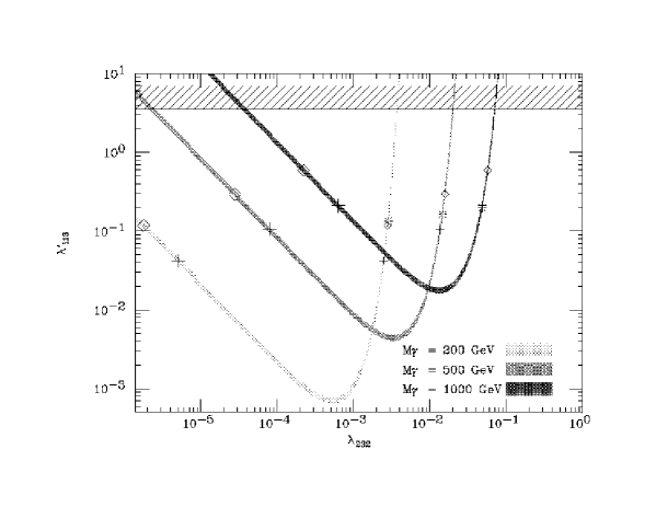
Using results for the RPV branching ratios of the B mesons and the neutralino lifetime we can find regions in parameter space, for a given sfermion mass, in which there are events inside the NuTeV detector, this is shown in Fig. 1.
This model can be tested at other experiments. At the NOMAD experiment for the same -meson branching ratio we obtain about an order of magnitude more events than at NuTeV. Thus our model can be completely tested by the NOMAD data! For neutralino production we are relying on a rare B-meson decay which can possibly be observed at a present or future B-factory although this may be difficult as the leptons produced will be very soft.
3 Conclusions
We have reconsidered the NuTeV di-muon observation in the light of supersymmetry with broken R-parity and neutral heavy leptons. We have shown that it is not possible to obtain the observed event rate with pair production of light neutralinos or via the production of neutral heavy leptons. However, we have introduced a new production method of neutralinos via -mesons. Due to the copious production of -mesons in the fixed target collisions the observed di-muon event rate can be easily obtained for allowed values of the R-parity violating couplings.
The model we have proposed can be completely tested using current NOMAD data. If the NOMAD search is negative our model is ruled out and the NuTeV observation is most likely not due to physics beyond the Standard Model.
4 Acknowledgments
A.D. would like to acknowledge financial support from the Network RTN European Program HPRN-CT-2000-00148 “Physics Across the Present Energy Frontier: Probing the Origin of Mass”.
Part XIII Kaluza-Klein States of the Standard Model Gauge Bosons:
Constraints From High Energy Experiments
K. Cheung and G. Landsberg
This contribution is a shortened version of the recent paper [214], with the focus on future high-energy facilities. The details of the formalism used to obtain the results presented here can be found in [214].
Recently, it has been suggested that the Planck, string, and grand unification scales can all be significantly lower than it was previously thought, perhaps as low as a few TeV [20, 215, 216, 217]. An interesting model was proposed [218, 219, 220, 221], in which matter resides on a -brane (), with chiral fermions confined to the ordinary three-dimensional world internal to the -brane and the SM gauge bosons also propagating in the extra dimensions internal to the -brane. (Gravity in the bulk is not of direct concern in this model.) It was shown [218] that in this scenario it is possible to achieve the gauge coupling unification at a scale much lower than the usual GUT scale, due to a much faster power-law running of the couplings at the scales above the compactification scale of the extra dimensions. The SM gauge bosons that propagate in the extra dimensions compactified on , in the four-dimensional point of view, are equivalent to towers of Kaluza-Klein (KK) states with masses (), where is the size of the compact dimension, is the corresponding compactification scale, and is the mass of the corresponding SM gauge boson.
There are two important consequences of the existence of the KK states of the gauge bosons in collider phenomenology. (i) Since the entire tower of KK states have the same quantum numbers as their zeroth-state gauge boson, this gives rise to mixings among the zeroth (the SM gauge boson) and the th-modes () of the and bosons. (The zero mass of the photon is protected by the U(1)EM symmetry of the SM.) (ii) In addition to direct production and virtual exchanges of the zeroth-state gauge bosons, both direct production and virtual effects of the KK states of the , and bosons would become possible at high energies.
In this proceedings, we study the effects of virtual exchanges of the KK states of the , and bosons in high energy collider processes. While the effects on the low-energy precision measurements have been studied in detail [222, 223, 224, 225, 226, 227, 228, 229], their high-energy counterparts have not been systematically studied yet. We attempt to bridge this gap by analyzing all the available high-energy collider data including the dilepton, dijet, and top-pair production at the Tevatron; neutral and charged-current deep-inelastic scattering at HERA; and the precision observables in leptonic and hadronic production at LEP 2.
We fit the observables in the above processes to the sum of the SM prediction and the contribution from the KK states of the SM gauge bosons. In all cases, the data do not require the presence of the KK excitations, which is then translated to the limits on the compactification scale . The fit to the combined data set yields a 95% C.L. lower limit on of 6.8 TeV, which is substantially higher than that obtained using only electroweak precision measurements. In addition, we also estimate the expected reach on in Run 2 of the Fermilab Tevatron and at the LHC, using dilepton production.
1 Interactions of the Kaluza-Klein States
We use the formalism of Ref. [219, 220, 221], based on an extension of the SM to five dimensions, with the fifth dimension, , compactified on the segment (a circle of radius with the identification ). This segment has the length of . Two 3-branes reside at the fixed points and . The SM gauge boson fields propagate in the 5D-bulk, while the SM fermions are confined to the 3-brane located at . The Higgs sector consists of two Higgs doublets, and (with the ratio of vacuum expectation values ), which live in the bulk and on the SM brane, respectively.
In the case of SU(2) U(1)Y symmetry, the charged-current (CC) and neutral-current (NC) interactions, after compactifying the fifth dimension, are given by [225]:
| (1) | |||||
| (2) | |||||
where the fermion currents are:
and ; and are the gauge couplings of the SU(2)L and U(1)Y, respectively; and . Here, we used the following short-hand notations: and , where is the weak-mixing angle. The tree-level (non-physical) and masses are and . Since the compactification scale is expected to be in the TeV range, we therefore ignore in the above equations the mass of the zeroth-state gauge boson in the expression for the mass of the -th KK excitation: , .
Using the above Lagrangians we can describe the two major effects of the KK states: mixing with the SM gauge bosons and virtual exchanges in high-energy interactions.
1.1 Mixing with the SM Gauge Bosons
The first few terms in the Eqs. (1) and (2) imply the existence of mixings among the SM boson () and its KK excitations (, ) where . There is no mixing for the fields because of the U(1)EM symmetry. These mixings modify the electroweak observables (similar to the mixing between the and ). The SM weak eigenstate of the -boson, , mixes with its excited KK states () via a series of mixing angles, which depend on the masses of and on the angle . The boson studied at LEP 1 is then the lowest mass eigenstate after mixing. The couplings of the to fermions are also modified through the mixing angles. The observables at LEP 1 can place strong constraints on the mixing, and thus on the compactification scale . Similarly, the properties of the boson are also modified.
The effects of KK excitations in the low-energy limit can be included by eliminating their fields using equations of motion. From the Lagrangians given by Eqs. (1) and (2) the masses and the low-energy CC and NC interactions are given by [225]:
In the following, we summarize the results presented in Refs. [223, 224, 225, 226, 227, 228, 229]. Nath and Yamaguchi [223] used data on , , and and set the lower limit on TeV. Carone [227] studied a number of precision observables, such as , , , leptonic and hadronic widths of the . The most stringent constraint on comes from the hadronic width of the : TeV. Strumia [226] obtained a limit TeV from a set of electroweak precision observables. Casalbuoni et al. [225] used the complete set of precision measurements, as well as and ’s from -N scattering experiments, and obtained a limit TeV. Rizzo and Wells [224] used the same set of data as the previous authors and obtained a limit TeV. Cornet et al. [229] used the unitarity of the CKM matrix elements and were able to obtain a limit TeV. Delgado et al. [228] studied a scenario in which quarks of different families are separated in the extra spatial dimension and set the limit TeV in this scenario.
1.2 Virtual Exchanges
If the available energy is higher than the compactification scale the on-shell production of the Kaluza-Klein excitations of the gauge bosons can be observed [230, 16]. However, for the present collider energies only indirect effects can be seen, as the compactification scale is believed to be at least a few TeV. These indirect effects are due to virtual exchange of the KK-states.
When considering these virtual exchanges, we ignore a slight modification of the coupling constants to fermions due to the mixings among the KK states and so we use Eqs. (1) and (2) without the mixings.******For the mixings are very small. Furthermore, they completely vanish for . This implies that any Feynman diagram which has an exchange of a , , , or will be replicated for every corresponding KK state with the masses where . Note that the coupling constant of the KK states to fermions is a factor of larger than that for the corresponding SM gauge boson, due to the normalization of the KK excitations.
The effects of exchanges of KK states can be easily included by extending reduced amplitudes. In the limit , the reduced amplitudes take the form:
based on which, the high energy processes can be described.
2 High Energy Processes and Data Sets
Before describing the data sets used in our analysis, let us first specify certain important aspects of the analysis technique. Since the next-to-leading order (NLO) calculations do not exist for the new interactions yet, we use leading order (LO) calculations for contributions both from the SM and from new interactions, for consistency. However, in many cases, e.g. in the analysis of precision electroweak parameters, it is important to use the best available calculations of their SM values, as in many cases data is sensitive to the next-to-leading and sometimes even to higher-order corrections. Therefore, we normalize our leading order calculations to either the best calculations available, or to the low- region of the data set, where the contribution from the KK states is expected to be vanishing. This is equivalent to introducing a -dependent -factor and using the same -factor for both the SM contribution and the effects of the KK resonances, which is well justified by the similarity between these extra resonances and the corresponding ground-state gauge boson. The details of this procedure for each data set are given in the corresponding section. Wherever parton distribution functions (PDFs) are needed, we use the CTEQ5L (leading order fit) set [231].
2.1 HERA Neutral and Charged Current Data
ZEUS [232, 233] and H1 [234, 235] have published results on neutral-current (NC) and charged-current (CC) deep-inelastic scattering (DIS) in collisions at GeV. The data sets collected by H1 and ZEUS correspond to integrated luminosities of 35.6 and 47.7 pb-1, respectively. H1 [234, 235] has also published a NC and CC analysis for the most recent data collected in collisions at GeV with an integrated luminosity of pb-1. We used single-differential cross sections presented by ZEUS [232, 233] and double-differential cross sections published by H1 [234, 235].
We normalize the tree-level SM cross section to that measured in the low- data by a scale factor ( is very close to 1 numerically). The cross section used in the fitting procedure is given by
| (3) |
where is the interference term between the SM and the KK states and is the cross section due to the KK-state interactions only.
2.2 Drell-Yan Production at the Tevatron
Both CDF [236] and D [237] measured the differential cross section for Drell-Yan production, where is the invariant mass of the lepton pair. (CDF analyzed data in both the electron and muon channels; D analyzed only the electron channel.)
We scale this tree-level SM cross section by normalizing it to the -peak cross section measured with the data. The cross section used in the fitting procedure is then obtained similarly to that in Eq. (3).
2.3 LEP 2 Data
We analyze LEP 2 observables sensitive to the effects of the KK states of the photon and , including hadronic and leptonic cross sections and forward-backward asymmetries. The LEP Electroweak Working Group combined the , and data from all four LEP collaborations [238] for the machine energies between 130 and 202 GeV. We use the following quantities in our analysis: (i) total hadronic cross sections; (ii) total cross sections; (iii) forward-backward asymmetries in the and channels; and (iv) ratio of -quark and -quark production to the total hadronic cross section, and . We take into account the correlations of the data points in each data set as given by [238].
For other channels we use various data sets from individual experiments. They are [239, 240, 241, 242, 243, 244, 245, 246, 247, 248, 249, 250, 251, 252, 253, 254]: (i) Bhabha scattering cross section ; (ii) angular distribution or forward-backward asymmetry in hadroproduction ; (iii) angular distribution or forward-backward asymmetry in the , , and production.
To minimize the uncertainties from higher-order corrections, we normalize the tree-level SM calculations to the NLO cross section, quoted in the corresponding experimental papers. We then scale our tree-level results, including contributions from the KK states of the and , with this normalization factor, similar to Eq. (3). When fitting angular distribution, we fit to the shape only, and treat the normalization as a free parameter.
2.4 Kaluza-Klein states of the Gluon in Dijet Production at the Tevatron
Since the gauge bosons propagate in extra dimensions, the Kaluza-Klein momentum conservation applies at their self-coupling vertices. Because of this conservation, the triple interaction vertex with two gluons on the SM 3-brane and one KK state of the gluon in the bulk vanishes. (However, the quartic vertex with two gluons on the SM 3-brane and two gluon KK states in the bulk does exist.) The cross sections for dijet production, including the contributions from KK states of the gluon, are given in Ref. [214].
2.5 Kaluza-Klein States of the Gluon in Production at the Tevatron
In Ref. [259], it was shown that production in Run 2 of the Tevatron can be used to probe the compactification scales up to TeV. In this paper, we consider the sensitivity from the existing Run 1 data by using the tree-level production cross section, including the contribution of the KK states of the gluon in the channel. (The channel does not have the triple vertex interaction with two gluons from the SM 3-brane and one KK state of the gluon in the bulk, as explained in the previous subsection.)
The latest theoretical calculations of the cross section, including higher-order contributions, at TeV correspond to 4.7 – 5.5 pb [260, 261]. The present data on the cross sections are [262, 263]
and the top-quark mass measurements are
In our analysis, we normalize the tree-level SM cross section to the mean of the latest theoretical predictions (5.1 pb), and use this normalization coefficient to predict the cross section in the presence of the KK states of the gluon (similar to Eq. (3)).
3 Constraints from High Energy Experiments
Based on the above individual and combined data sets, we perform a fit to the sum of the SM prediction and the contribution of the KK states of gauge bosons, normalizing our tree-level cross section to the best available higher-order calculations, as explained above. The effects of the KK states always enter the equations in the form [214]. Therefore, we parameterize these effects with a single fit parameter . In most cases, the differential cross sections in the presence of the KK states of gauge bosons are bilinear in .
The best-fit values of for each individual data set and their combinations are shown in Table 1. In all cases, the preferred values from the fit are consistent with zero, and therefore we proceed with setting limits on . The one-sided 95% C.L. upper limit on is defined as:
| (4) |
where is the fit likelihood function given by . The corresponding upper 95% C.L. limits on and lower 95% C.L. limits on are also shown in Table 1.
| (TeV-2) | (TeV-2) | (TeV) | |
|---|---|---|---|
| LEP 2: | |||
| hadronic cross section, ang. dist., | 0.12 | 5.3 | |
| cross section & ang. dist. | 0.42 | 2.8 | |
| cross section & ang. dist. | 0.16 | 4.5 | |
| LEP combined | 0.076 | 6.6 | |
| HERA: | |||
| NC | 1.59 | 1.4 | |
| CC | 2.45 | 1.2 | |
| HERA combined | 1.25 | 1.6 | |
| TEVATRON: | |||
| Drell-Yan | 1.96 | 1.3 | |
| Tevatron dijet | 1.0 | 1.8 | |
| Tevatron top production | 9.2 | 0.60 | |
| Tevatron combined | 0.65 | 2.3 | |
| All combined | 0.071 | 6.8 |
4 Sensitivity in Run 2 of the Tevatron and at the LHC
At the Tevatron, the best channel to probe the KK states of the photon or the boson is Drell-Yan production. In Ref. [264], we showed that using the double differential distribution can increase the sensitivity to the KK states of the graviton compared to the use of single-differential distributions. Similarly, we expect this to be the case for the KK states of the photon and the boson.
We follow the prescription of Ref. [264] and use the Bayesian approach, which correctly takes into account both the statistical and systematic uncertainties, in the estimation of the sensitivity to .††††††Note that the maximum likelihood method, as given by Eq. (4), artificially yields 10% higher sensitivity to , as it does not properly treat the cases when the likelihood maximum is found in the unphysical region . Due to the high statistics in Run 2 and particularly at the LHC, the overall systematics becomes dominated by the systematics on the -dependence of the -factor from the NLO corrections. (Systematic uncertainties on the integrated luminosity and efficiencies are not as important as before, because they get canceled out when normalizing the tree level SM cross section to the -peak region in the data.) The uncertainty on the -factor from the NLO calculations for Drell-Yan production [265] is currently known to a 3% level, so we use this as the correlated systematics in our calculations on . For the LHC we quote the limits for the same nominal 3% uncertainty and also show how the sensitivity improves if the uncertainty on the -factor shape is reduced to a 1% level. It shows the importance of higher-order calculations of the Drell-Yan cross section, which we hope will become available by the time the LHC turns on.
In the simulation, we use a dilepton efficiency of 90%, a rapidity coverage of , and typical energy resolutions of the Tevatron or LHC experiments. The simulation is done for a single collider experiment in the combination of the dielectron and dimuon channels.
As expected, the fit to double-differential cross sections yields a better sensitivity to than just using one-dimensional differential cross sections. We illustrate this by calculating the sensitivity to in Run 1, which is slightly higher than the result obtained from the fit to the invariant mass spectrum from CDF and D. The sensitivity, at the 95% C.L., to in Run 1 (120 pb-1), Run 2a (2 fb-1), Run 2b (15 fb-1), and at the LHC (100 fb-1) is given in Table 2. While the Run 2 sensitivity is somewhat inferior to the current indirect limits from precision electroweak data, LHC would offer a significantly higher sensitivity to , well above 10 TeV.
| (TeV-2) | 95% C.L. lower limit on (TeV) | |
|---|---|---|
| Run 1 (120 pb-1) | 1.62 | 1.4 |
| Run 2a (2 fb-1) | 0.40 | 2.9 |
| Run 2b (15 fb-1) | 0.19 | 4.2 |
| LHC (14 TeV, 100 fb-1, 3% systematics) | 13.5 | |
| LHC (14 TeV, 100 fb-1, 1% systematics) | 15.5 |
5 Acknowledgments
We would like to thank Ignatios Antoniadis, Keith Dienes, JoAnne Hewett, Steve Mrenna, Giacomo Polesello, and Tom Rizzo for useful discussions. Many thanks to the Les Houches organizers for making it a very productive scientific workshop. This research was partially supported by the U.S. Department of Energy under Grants No. DE-FG02-91ER40688 and by A.P. Sloan Foundation, and by the National Center for Theoretical Science under a grant from the National Science Council of Taiwan R.O.C.
Part XIV Kaluza-Klein Excitations of Gauge Bosons in
the ATLAS Detector
G. Azuelos and G. Polesello
1 Introduction
In models with “large” Extra Dimensions, characterized by compactification radii , gravity propagates in the bulk, and the SM fields are confined to a 3-brane. The presence of the Extra Dimensions could be probed by searching for the Kaluza-Klein excitations of the gravitons at the future high energy accelerators, and these scenarios have been the subject of many phenomenological studies. An interesting variation of the ADD model [218, 219, 220, 221] assumes that only the fermions are confined in the 3-brane, whereas the gauge fields propagate in a number of additional “small” extra dimensions orthogonal to the brane with compactification radius TeV.
For definiteness we concentrate here on a model with only one “small” extra dimension, and where all of the SM fermions are on the same orbifold point (). The phenomenology of this model, which we will label as M1 is discussed in some detail in [230]. For compactification on dimension, the model is completely specified by a single parameter , the compactification scale, and the masses of the KK modes of the gauge bosons are given by the relation , where is the mass of the zero-mode excitation corresponding to the Standard Model gauge boson. The couplings are the same as the corresponding SM couplings, scaled by a factor . As an example of variation on our reference model we also briefly consider an alternative model, [21] (M2), where quark and leptons are at opposite fixed points. The difference between the reference model and M2 is that for model M2 the signs of the quark couplings of the bosons are reversed for excitations with odd, yielding a different interference pattern with the SM Drell-Yan production.
The constraints on the compactification scale from precision electroweak measurements have been evaluated in a number of papers, [230, 266, 223, 225, 224, 227, 228, 229]. These studies estimate an approximate lower limit of 4 TeV on the compactification scale for the reference model considered in this analysis. A recent paper [214, 267] calculates the limits which can be extracted from precision measurements at present high-energy accelerators. A 95% limit of 6.8 TeV is obtained, dominated by the LEP 2 measurements. The limit, however, comes from the fact that for two of the three fits to LEP data, an unphysical negative value for is obtained, with a significance of two to three standard deviations. In view of this fact, waiting for a clarification of the claimed discrepancy with the Standard Model, we conservatively study the performance of the ATLAS detector starting from TeV.
2 Signal simulation and data analysis
We simulate at particle level the production of the gauge boson excitations, including the full interference and angular information. We include the full Breit-Wigner shape for the first two excitations of and [268], and a resummed expression for the higher lying states, for which the approximation is used. The expression with only the first two resonances, does not alter the results for the reach in the peak region, but it significantly underestimates the deviation from the Standard Model in the low mass off-peak region. Since the dominant contributions to the low off-resonance region comes from the interference term between SM and the excitations, the deviation from the SM is approximately proportional to:
| (1) |
Therefore the deviation from the SM increases by when the full tower of resonances is considered instead of just the first two. If we consider model , the sum over the tower of resonances gives a term proportional to
Therefore, the summed contribution of the interference terms in model M2 will be of opposite sign and half of the one for the reference model. The matrix elements are interfaced to PYTHIA 6.125 [113] event generator as an external process, and full events have been generated, including the full PYTHIA machinery for QCD showering from the initial state quarks, and for the hadronization.
The events thus generated have been passed through the fast simulation of the ATLAS detector [269]. As discussed in the introduction, the lowest considered in this study is 4 TeV, consistent with precision electroweak measurements. Therefore we need to detect and measure leptons with momenta in the few TeV range. In this range the energy resolution for electrons is dominated by a constant term due to the imperfect knowledge of the detector performance. From studies performed on test beam data and on fully simulated events, for energies up to a few hundred GeV, this term has been evaluated as a few per mill. Detailed studies need to be performed to evaluate how well these results extrapolate to the momentum range of interest for this analysis. With this caveat, we use here the standard parametrization included in the ATLFAST program which yields a resolution of 0.7% for the energy measurement of 2 TeV electrons. For muons the transverse momentum measurement of high muons is achieved through the sagitta measurement in the precision drift chambers, and for a 2 TeV muon the resolution is of order 20%. Considering the natural widths of the gauge excitations, the width of the lepton-lepton invariant mass distribution will be dominated by the natural width for electrons, and by the experimental momentum resolution for muons. This is illustrated in Figure 1 where the invariant mass spectra for a 4 TeV KK resonance is shown both for electrons (full line) and muons (dashed line). Although the muon peak is much broader, both lepton species can be used in order to observe the existence of an excess in the peak region with respect to the Standard Model.
Comparing the two-lepton invariant mass spectrum for Standard Drell-Yan production (full line), and for the reference model (dashed line) as shown in Fig.2, two basic features can be observed:
-
•
A peak centered around , corresponding to the superposition of the and Breit-Wigner shapes
-
•
A suppression of the cross-section with respect to the SM for masses below the resonance. This suppression is due to the negative interference terms between the SM gauge bosons and the whole tower of excitations, and is sizable even for compactification masses well above the ones accessible to a direct detection of the mass peak. This shape is the consequence of the model choices requiring both the leptons and the quarks to be at the same orbifold point (D=0). The different model choices corresponding to M2 would yield an enhancement of the off peak cross-section, as shown in the dotted line in Fig. 2.
We select events with two isolated opposite sign leptons, satisfying the following requirements:
-
•
GeV ()
-
•
GeV,
The isolation criterion consists in requiring a transverse energy deposition in the calorimeter smaller than 10 GeV in a () cone of radius 0.2 around the lepton direction. In the absence of new physics, approximately 500 events survive these cuts for an integrated luminosity of 100 fb-1, corresponding to one year of high luminosity LHC running for each of the lepton flavors.
The reach for the observation of a peak in the distribution can be naively estimated from Table 1, which, for both electrons and muons gives the number of signal and background events for an integrated luminosity of 100 fb-1 for different values of . As an arbitrary requirement for discovery we ask for the detection above a given of 10 events summed over the two lepton flavors, and a statistical significance . The reach thus calculated is 5.8 TeV for an integrated luminosity of 100 fb-1. In order to achieve this reach, a good control of high background events which might be produced by the mismeasurement of leptons is crucial. A handle on these events is however provided by the consideration of the momentum balance of the event in the transverse plane, which will allow to reject events with one badly mismeasured lepton.
Unfortunately, even for the lowest allowed value of , 4 TeV, no events would be observed for the second resonance at 8 TeV, which would have been the most striking signature for this kind of model.
| (GeV) | Cut (GeV) | Background () | Background () | ||
|---|---|---|---|---|---|
| 4000 | 3000 | 172 | 156 | 1.45 | 1.8 |
| 5000 | 4000 | 23 | 20 | 0.15 | 0.22 |
| 5500 | 4000 | 9 | 8 | 0.15 | 0.22 |
| 6000 | 4500 | 3.3 | 2.8 | 0.05 | 0.1 |
| 7000 | 5000 | 0.45 | 0.38 | 0.015 | 0.05 |
| 8000 | 6000 | 0.042 | 0.052 | 0.0015 | 0.012 |
In order to fully evaluate the sensitivity of the invariant mass spectrum off-resonance to interference effects, a likelihood fit to the expected spectrum can be performed, and will be discussed in the next section. As a first approach, one can simply evaluate the variation in number of events within a given range with respect to the SM, as a function of . We show the invariant mass spectrum between 1000 and 2000 GeV in Figure 3 for Standard Model and for three choices of .
A naive parameterization of the statistical significance of the cross-section suppression is
A relevant variable which should also be considered is the ratio , because the systematic uncertainty in our knowledge of the shape of sets a limit on the detectable value of this ratio. The choice of the mass interval is subject to the consideration of the systematical uncertainty, as the statistical significance somewhat increases by lowering the lower limit of the considered mass window, at the price of a worse . We choose for this analysis a mass interval GeV.
From the numbers in Table 2,
if we consider both lepton flavors, the ATLAS 5 reach is 8 TeV
for an integrated luminosity of 100 fb-1 and 10.5 TeV
for 300 fb-1. The deviation from the Standard Model
will be 16% for 8 TeV, and for 10.5 TeV,
defining in each case the level of systematic control
on the relevant region of the lepton-lepton invariant mass spectrum
we need to achieve to exploit the statistical power of the data.
| (GeV) | |
|---|---|
| SM | 483 |
| 4000 | 210 |
| 5000 | 295 |
| 5500 | 324 |
| 6000 | 349 |
| 7000 | 381 |
| 8000 | 405 |
| 8500 | 413 |
| 9000 | 419 |
| 10000 | 432 |
| 11000 | 443 |
| 12000 | 450 |
3 Optimal reach and mass measurement
In the previous sections we have evaluated in a naive way by simple event counting the range within which LHC will be able to observe a peak generated by the KK gauge excitations, and/or a deviation from the Standard Model in the distribution off-peak. An optimal estimate of the reach can be obtained by performing a likelihood fit to the invariant mass shape expected for different values of . Instead of using just the invariant mass, we use the full information contained in the events. Ignoring the transverse momentum of the system, the event kinematics for a given event is defined by the variables . The values of , have been evaluated from the four-momenta of the detected electrons, according to the formulas:
For the evaluation of we use the Collins-Soper convention [270], consisting in the equal sharing of the system transverse momentum between the two quarks. A basic problem for the likelihood calculation is the fact that, as the LHC is a collider, it is not possible to know from which direction the quark in the hard scattering comes from, so only the absolute value of can be measured, but not its sign. Part of this information can however be recovered, by using the knowledge of and and the fact that in the proton the distribution for valence quarks is harder than for anti-quarks. A detailed discussion of the experimental reconstruction of the three variables is given in [271].
For the processes under study, the initial state is for both signal and background, so the optimal result can be obtained by just using the two physical variables sensitive to the dynamics of the hard-scattering processes, namely and . However, since for electrons the effect of the experimental smearing is small, an effective approach to the problem is to use the theoretical cross-section expression to build an unbinned likelihood. In this approach, the use of only two variables would require an integration over the third one for each step in the likelihood calculation for each Monte Carlo experiment, making the process unacceptably slow. For muons the experimental smearing must be taken into account, and the fit can be performed by building an event density grid in the plane.
In the following we will only perform the likelihood fit for electrons,
calculating the unbinned likelihood functions on event samples
corresponding to an integrated luminosity of 100 fb-1.
In order to evaluate the uncertainty on the measurement,
for each input value we generated an ensemble of Monte Carlo experiments
(100 fb-1 each) and for each of them we estimated
by maximizing the likelihood function.
The likelihood fit is performed on the variable , since
for it is the natural variable for describing
the deviation of the cross-section from the Standard Model, as shown
in Eq. 1.
With the use of this test variable,
the Standard Model is the limit corresponding to ,
and it is possible to build a continuous likelihood function extending
the evaluation to unphysical negative values of .
We show in Figure 4 the distributions of the estimated values of for four input values of . As expected, the distributions are gaussian as long as events in the peak exist, and tails start to appear for =6 TeV for which, on average, only three events appear in the peak region for the considered statistics. For =7 TeV, less than 1 event is observed in the peak and the distribution becomes very broad, with an RMS corresponding to 600 GeV, and large tails. The average and RMS of the estimated value of are given in Table 3. The statistical error is below the percent level as long as events are observed in the peak region. A small systematic shift in the average of the estimated is observed, due to the fact that the likelihood is built using analytical test functions neglecting detector smearing and transverse motion of the system.
| (GeV) | (GeV) | RMS |
|---|---|---|
| 4000. | 4001.96 | 10.91 |
| 5000. | 5003.16 | 35.91 |
| 5500. | 5502.19 | 77.24 |
| 6000. | 6045.22 | 216.61 |
| 7000. | 7129.48 | 544.35 |
The experimental sensitivity is defined in [272] as the average upper limit that would be attained by an ensemble of experiments with the expected background and no true signal. To evaluate the sensitivity, we therefore produced an ensemble of Monte Carlo experiments for which only SM Drell-Yan was generated. For the evaluation of the 95% CL limit for each MonteCarlo experiment we use the following prescription. For each Monte Carlo experiment we build the likelihood function as a function of 1/ as described above. We then define as 95% CL limit the value of such that the integral of between zero and 1/ is 95% of the integral between zero and infinity. The experimental sensitivities for one lepton flavor thus obtained are respectively 9.5, 11 and 12 TeV for integrated luminosities of 100, 200 and 300 fb-1. These values are pessimistic, since they do not take into account the systematic deviation from zero of the estimated 1/ value due to the approximate test function used to perform the study. Correcting for the deviation from zero yields an improvement of approximately 200 GeV on these numbers. If we assume similar sensitivity for electrons and muons, the sensitivity is 13.5 TeV for 300 fb-1 and both lepton species. These figures only express the statistical sensitivity of the ATLAS experiment, the possible sources of systematic uncertainty must be considered in order to evaluate the final ATLAS sensitivity.
4 Systematic uncertainties
As shown in the the previous section, the effect of KK excitation can be detected for well above the mass range for which the direct observation of a peak is possible from a detailed study of the event shape in the interference region. The experimental sensitivity in this region crucially depends on our understanding of the kinematic distributions of the lepton-lepton system both under the experimental and the theoretical point of view.
As shown in Figure 3, as increases, the difference in shape with respect to the standard model becomes less and less significant, and systematic effects in the lepton-lepton invariant mass measurement might affect the shape of the distribution, and destroy the experimental sensitivity. We consider for this analysis electrons of very high momentum, around 1 TeV. At this energy scale the linearity of the lepton momentum measurement, as well as the momentum dependence of the acceptance are difficult to assess using the data. In fact very few of the leptons from the decay of high momentum W and Z, which could in principle be used to perform the measurement will have high enough momentum. From studies performed for lepton calibration in ATLAS, we know that the lepton energy scale will be known to 0.1% at the mass. We therefore parametrize the deviation from linearity as a logarithmic term which is zero for lepton momentum of 100 GeV, and 1 or 5% for momenta of 2 TeV. We perform the likelihood analysis on all our simulated data samples, modifying event by event the reconstructed lepton energy according to the logarithmic formula. For the evaluation of between 4 and 6 TeV, the relative deviation from the nominal approximately scales with the deviation from linearity for 2 TeV leptons, as shown in Fig.5 for 3 values of : 4, 5 and 5.5 TeV.
The variation of the sensitivity with the assumed value of the deviation from linearity is shown in Figure 6.
As discussed above, the systematic uncertainty is reflected in a systematic shift of the average estimate, and an overestimate of the lepton calibration is going to yield an optimistic evaluation of the value excluded by the experiment. Taking the sensitivity values obtained with a negative deviation from linearity, the sensitivity for 100 fb-1 and one lepton species is reduced from 9.5 TeV to 9.3 TeV and 8.75 TeV for 1 and 5% deviation respectively. As an approximate rule, the experimental limit should be reduced by 2% for each percent of uncertainty on the energy calibration of 2 TeV leptons.
An additional uncertainty factor is the theoretical systematics on the likelihood calculation. The likelihood function is built by weighting real events according to a theoretical cross-section formula. Any discrepancy between the theoretical formula employed and reality will induce an uncertainty on the measurement of . In the likelihood analysis we are not sensitive to an absolute -factor, since we do not use the absolute normalization, but only to distortions of the kinematic distributions of the lepton-lepton system. Three main sources of uncertainty can be identified:
-
•
QCD higher order corrections;
-
•
electroweak higher order corrections;
-
•
the parton distribution function (PDF) for the proton.
The main effect of QCD higher order corrections is the modification of the distribution of the lepton-lepton pair, due to radiation from initial state quarks. This effect is taken into account in a very pessimistic way in the study on fully generated events, where the likelihood is built from the leading order 2-to-2 Drell-Yan expression, and the events are generated with the full PYTHIA machinery for initial state radiation. Therefore, the experimental error quoted in the previous section includes a very pessimistic estimate of this effect. In fact in a real experiment a more realistic theoretical modelling will probably be used to build the likelihood.
Electroweak higher order corrections were recently calculated at NLO [273], and shown to be sizable, leading to a reduction of the cross-section which varies with the lepton-lepton invariant mass, and can be as large as 35% for and . The size of these corrections critically depends on the lepton identification and isolation criteria, as a substantial part of the higher order effects yield energetic photons produced alongside the leptons. The evaluation of the uncertainties on these corrections is thus a complex interplay of experimental and theoretical considerations which requires a dedicated study which is outside the scope of this analysis.
The shape of the kinematic distributions of the lepton-lepton system, in particular has a strong dependence on the quark and antiquark PDF’s in particular for high values of . All the events were generated with the CTEQ4L PDF’s. In order to evaluate the effect of the uncertainty on the structure functions parametrization, the likelihood fit was performed on the data set thus generated, using a number of structure function sets. To this purpose we have selected the sets providing a leading order parametrization, and which are based on the latest available data sets. The distributions of estimated masses are shown in Fig.7 for the eight choices of structure function sets used for and 5.5 TeV.
The systematic displacement from the true value is between 3 and 4 GeV for 4 TeV, increasing to 10-20 GeV for 5 TeV and 20-40 GeV for 5.5 TeV, and it is well below the RMS of the distributions given in Table 3. Another notable effect is that the quality of the likelihood fit is worse, giving rise to less Gaussian distributions, and sizable tails start to appear for TeV. The experimental reach for 100 fb-1 is shown in Fig. 8, as a function of the structure function set. In the worst case the reach is reduced by GeV with respect to CTEQ4L.
5 Spin and Asymmetry Measurement
If a Kaluza-Klein gauge excitation is discovered, one of the ways of distinguishing the signal from a , predicted by GUT theories, or from a narrow graviton resonance is by the angular distribution of the decay products, which should be consistent with the spin 1 nature of the excitation, and by the forward-backward asymmetry. By adjusting parameters of the models, the cross sections can be made comparable, but, as shown above and in [274], the shape of the mass distribution can provide an additional distinguishing criterion. The present study compares these distributions, but does not attempt to distinguish the resonances by the shape of their mass distributions, by their relative cross sections, nor by the branching ratios.
5.1 Cases studied
We studied the following cases
-
a)
: this is the case of gauge excitations, model M1 [230], at mass 4 TeV. The process was implemented in PYTHIA 6.201.
-
b)
-M2: this case of gauge excitation is with the alternative model M2 [21], also at 4 TeV. The process was implemented in PYTHIA
-
c)
: this is a standard model . The same code as for case a) was used, but the first excitation and higher excitations of and were removed.
-
d)
: This is the case of a narrow graviton resonance, as was studied by [275]. The process is implemented in PYTHIA. In order to reproduce a resonance of width comparable to the of a) above, the dimensionless coupling which enters in the partial widths of the (PARP(50) in PYTHIA) was set to 0.8. The reconstructed width is thus GeV. The angular distributions depend on the incoming partons. The two processes and were generated and added in proportion of their cross section. To their sum was added the Standard Model Drell-Yan background .
The mass distributions normalized to a luminosity of 100 fb-1 are displayed in Figs. 9 for the different cases. The cross sections for the different processes are summarized in table 4.
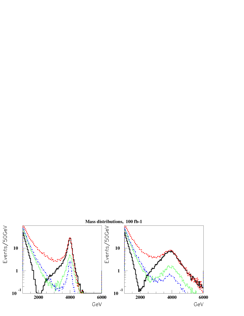
| process | (fb) |
|---|---|
| 4.05 | |
| -M2 | 11.75 |
| 4.65 | |
| 0.20 | |
| 0.13 | |
| 4.83 |
5.2 Angular Distributions
As mentioned above, because the colliding particles at LHC are both protons, the forward-backward asymmetry is measured with some ambiguity. Assuming that the resonances are produced by fusion, the third component of the reconstructed momentum of the dilepton system is taken to be the quark direction, since the quark in the proton is expected to have higher energy than an antiquark from the sea.
Events around the peak of the resonance were selected: 3750 GeV 4250 GeV or 3250 GeV 4750 GeV. For these events, the cosine of the angle of the lepton ( or ), with respect to the beam direction, in the frame of the decaying resonance, is shown in Figs. 10 and 11. The positive direction is defined by the sign of the reconstructed momentum of the dilepton system. Since we will be interested only in the shape, and not in the cross sections, the angular distribution histograms have been normalized, to a total of 138 events, corresponding to the number of events predicted with an integrated luminosity of 100 fb-1 for the reference case .
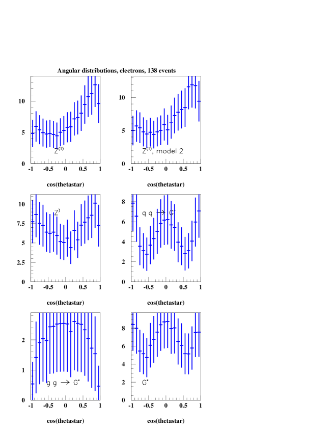
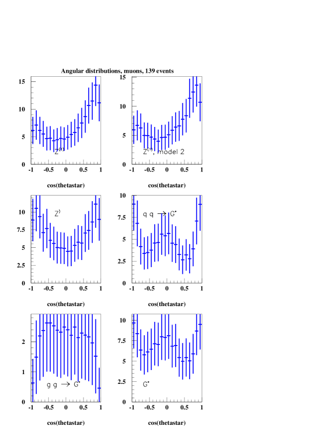
To compare the shape of these distributions, a set of 1000 angular distributions from the different types of resonances was generated by sampling from the expected distributions of Figs. 10 and 11. A Kolmogorov test was then applied‡‡‡‡‡‡In principle, the Kolmogorov test should be applied on unbinned data, but the application on binned data should still provide a valid test, in the present case since the bins are narrower than the expected features between the expected distribution and distributions sampled from the other resonances. The output of the test is expected to be a uniform distribution between 0 and 1 if they come from the same parent distribution. The histogram of the outputs is displayed in Fig. 12. No significant difference is found between models M1 and M2 of , as expected. However, the Kolmogorov test, applied to the distributions obtained for the channel, will give an average probability of consistency between and or between and of 0.105 and 0.015 respectively and will reject, at 95% confidence level, the hypothesis that the distributions derive from the same parent distribution 52% and 94% of the times. For higher resonance masses the statistical significance quickly decreases: at 5 TeV, with only 18 events in the peak region, no discrimination becomes possible. However, for this mass but with an integrated luminosity of 300 fb-1, the Kolmogorov test would reject the hypothesis, at 95% CL, about 20% of the times. Similar results are obtained for the channel.
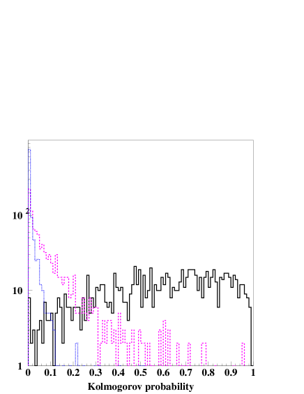
A test was also performed between these distributions, leading to the same conclusions. Here, also, a histogram of the calculated was produced from a sample of 1000 pseudo experiments with 138 events each. The average /d.f. are 0.998, 1.50 and 2.10 for the cases of model M2, and respectively. The goodness of fit test between the and the or angular distributions would yield a confidence level below 5% respectively 38% and 84% of the times.
5.3 Forward-backward asymmetry
From the angular distributions, the forward-backward asymmetry is obtained and shown in Figs. 13 and 14 as a function of the reconstructed dilepton mass. It allows a clear distinction between a resonance due to and either a or a resonance. Indeed, the asymmetry is expected to be close to at the mass peak of the , if the couplings are those of the SM, because :
| (2) | |||||
| with | (3) | ||||
| (4) |
For masses below, but close to the resonance, the FB asymmetry can also serve as a distinguishing criterion between the and the . For large masses, however, the discrimination power becomes quickly limited by statistics.
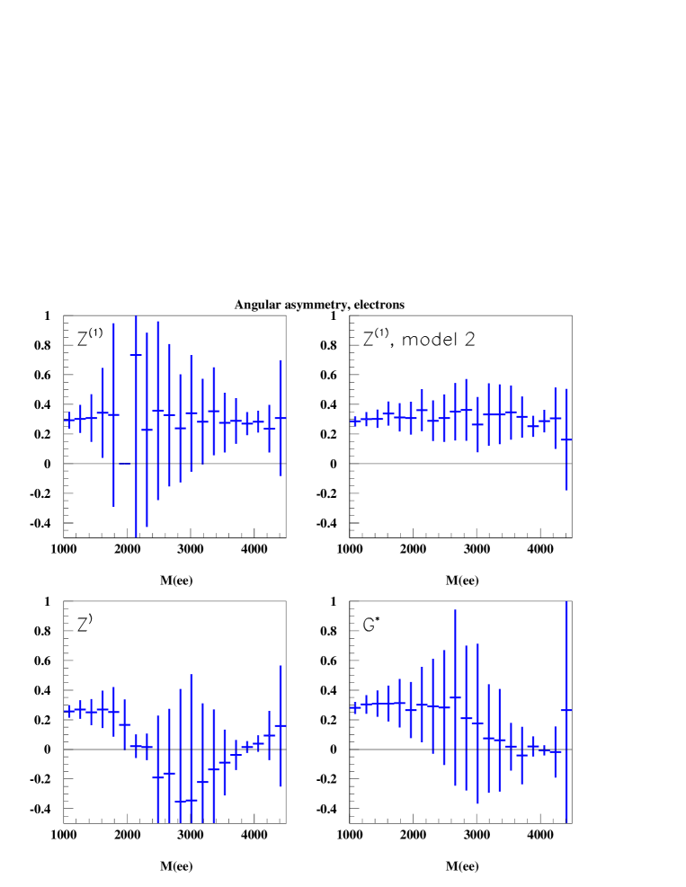
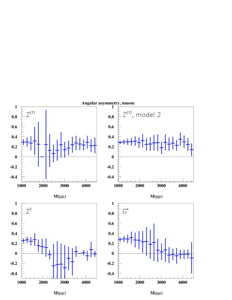
6 Conclusions
We have performed a detailed study of the leptonic signatures for the production of the KK excitations of the and in models with TeV-scale extra-dimensions.
The production and decay of the excitations were fully simulated, including initial state QCD radiation, and the resulting particles were passed through a parametrized simulation of the ATLAS detector.
We found that with an integrated luminosity of 100
ATLAS will be able to detect a peak in
the lepton-lepton invariant mass if
the compactification scale () is below 5.8 TeV.
Even in the absence of a peak,
a detailed study of the shape of the lepton-lepton invariant mass
will allow to observe a deviation from the standard model
due to the interference of the KK excitations with the SM
bosons.
From a study based on a maximum likelihood estimation
of the compactification mass, ATLAS
will be able to exclude at 95% CL a signal from the models
considered in this work for TeV
with an integrated luminosity of 300 .
We have performed an evaluation of the influence of
experimental and theoretical uncertainties on this result.
A 1% deviation from linearity in lepton momentum measurement
yields a 2% reduction in sensitivity.
The maximum effect observed from the consideration of various
sets of PDF’s is a reduction of order 200 GeV on the
achievable limit.
Once a peak is observed, an important question is the assessment of the model which has produced the signal. We show that for resonances of mass up to 5 TeV, and with an integrated luminosity of 300 , the KK excitations can be distinguished from mass peaks produced by SM-like or graviton resonances from the study of the polar angle distribution of the leptons in the peak region. The forward-backward lepton asymmetry as a function of invariant mass can provide a more general distinguishing criterion among the different models. For invariant masses around the peak, it will allow to distinguish the KK excitations from alternative models yielding the same signature.
Part XV Search for the Randall Sundrum Radion Using the ATLAS Detector
G. Azuelos, D. Cavalli, H. Przysiezniak, L. Vacavant
1 Introduction
Theories with extra dimensions have recently received considerable attention. One of the most interesting incarnations was formulated by Randall and Sundrum (RS) [4], who postulate a universe with two 4-d surfaces (branes) bounding a slice of 5-d spacetime. The SM fields are assumed to be located on one of the branes (the TeV brane), while gravity lives everywhere: on the TeV brane, on the Planck brane and in the bulk. The metric is exponentially warped in the fifth dimension, allowing for a natural resolution of the hierarchy problem.
The theory admits two types of massless excitations: the usual 4-d graviton and a graviscalar. In order to stabilize the size of the extra dimension without fine tuning of parameters, Goldberger and Wise (GW) [19] have proposed a mechanism which requires a massive bulk scalar , the radion, expected to be lighter than the J=2 Kaluza Klein excitations. The presence of the radion is one of the important phenomenological consequences of these theories of warped extra dimensions [276, 277, 278, 279]. The study of this scalar therefore constitutes a crucial probe of the model.
1.1 Radion branching ratios and width
The radion couplings to fermions and bosons are similar to those of the Standard Model (SM) Higgs [276]. They are expressed as a function of three parameters: the mass of the radion , the vacuum expectation value of the radion or scale, , and , the radion-SM Higgs mixing parameter [276, 280].
In the following study, we assume that the SM Higgs has been discovered and that its mass has been measured. The branching ratios of the radion are calculated using those of the SM Higgs as calculated in HDECAY [150], and using the ratio of the radion to Higgs branching ratios given by [276].
Figure 1 shows the principal branching ratios as a function of scalar mass for decays of the SM Higgs (top plots) and of the radion when GeV and 1 TeV, for when there is no -h mixing (middle plots), and for when and h are heavily mixed (bottom plots). We note the following:
-
•
BR() is greatly enhanced with respect to the Higgs and is close to unity for GeV and
-
•
the radion decays into two SM Higgs for
-
•
BR() is enhanced for and GeV.
For and for a radion with mass close to that of the Higgs, a strong interference produces a strong suppression of decays to vector bosons.
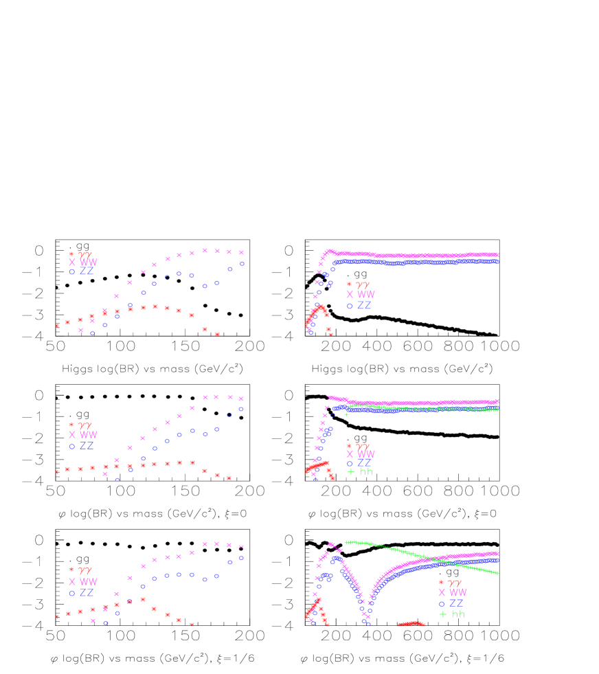
The radion has a very narrow natural width. Figure 2 shows the total width as a function of mass, for the SM Higgs and for the radion with and 1/6, for 1 TeV. The width is inversely proportional to the square of .
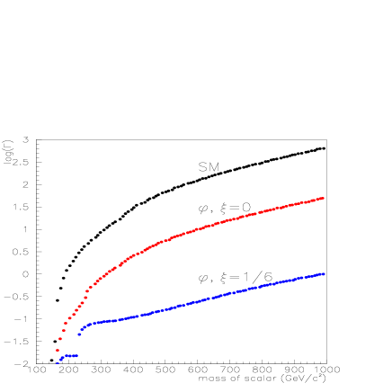
The aim of the present study is to investigate the possibility of observing a RS radion with the ATLAS detector through the following decays: , , and . Only the direct production of the radion is considered.
2 and
For the () and ZZ(∗) () decay channels, the radion signal significance is determined from the SM Higgs results obtained in the ATLAS TDR [97], for 100 fb-1 (one year at high luminosity ). The ratio of the radion over that of the SM Higgs is given by [276]:
where the mass resolutions are given by and . Using the ATLAS TDR SM Higgs signal significance results, the radion signal significance is determined and shown versus the mass of the radion, in Figure 3, for the channel (top) and for the ZZ(∗) channel (bottom), for 1,10 TeV, =0,1/6, and for an integrated luminosity of 100 .
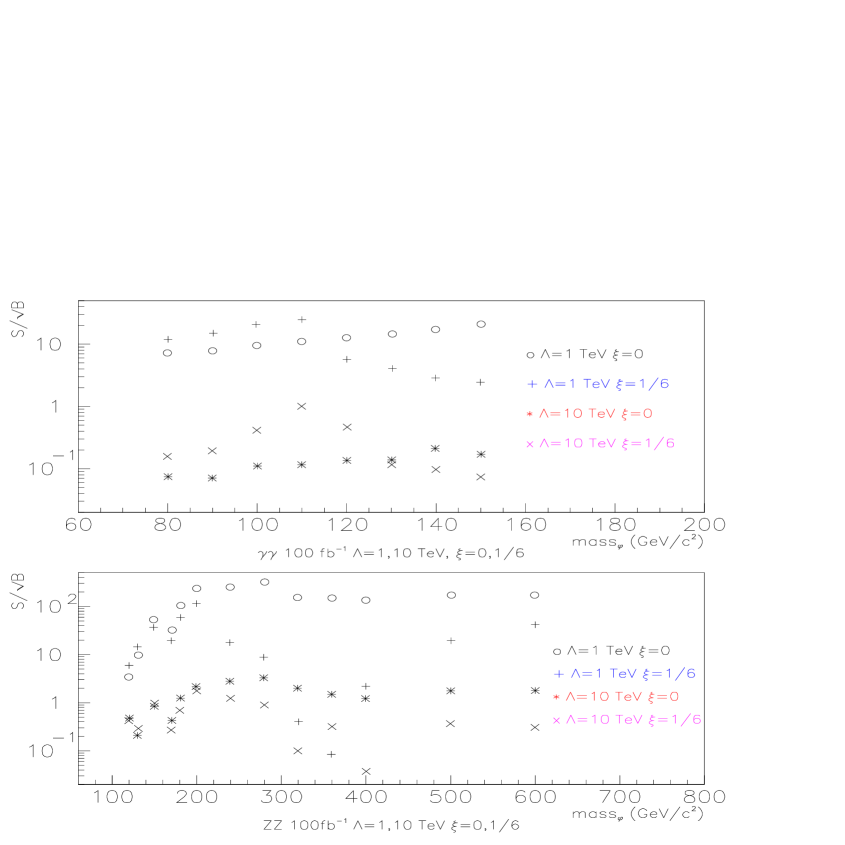
3
The radion, unlike the SM Higgs but similarly to the ones in the Minimal Supersymmetric Standard Model (MSSM), decays into Higgs pairs with relatively high BR (see Figure 1). As shown in Figure 2, the total width of the radion is a factor of 10 (100) smaller for 0 (1/6) than that of the Higgs, such that it is completely negligible with respect to the reconstructed mass resolutions.
The specific decay channel offers an interesting signature, with two high- isolated photons and two b-jets. The background rate is expected to be very low for the relevant mass region GeV/ and . In addition, triggering on such events is easy and the diphoton mass provides very good kinematical constraints for the reconstruction of .
The decay was studied in the context of the MSSM Higgs [281], although at that time the mass ranges investigated were lower. The approach and the selection we use in this study are very similar.
3.1 Signal
Signal events were generated with PYTHIA 6.158 [113]. The modified version of HDECAY described in Section 1.1 is used at the initialization phase to input the correct parameters and at the end of the run to re-scale the cross-section. Note that the default PYTHIA parameters, as opposed to the HDECAY ones, are used for the light Higgs couplings and parameters.
The heavy Higgs production process via gluon-gluon fusion (in the framework of the Minimal 1-Higgs doublet Standard Model, process ISUB=152) is used to produce the radion. The mass of the was set to reflect that of the radion, and the light Higgs mass was set to GeV. In addition, since the width of the radion is much narrower than what is usually encountered in a Higgs scenario, a specific correction was implemented [282] and the branching ratio corrected appropriately. Two samples of 100k events each were generated, for GeV/ and for GeV/.
3.2 Background
The backgrounds for this channel are (irreducible), , , and (reducible with b-tagging). The events were generated with PYTHIA 6.158. The main production process is the box diagram (process ISUB=114), where the jets arise from initial state radiation, eventually combined with gluon splitting for heavy flavor jets. The rates are therefore very low. However large uncertainties apply to these backgrounds since the jet part comes only from radiation and not from the hard-scattering. Generating a background sample of a sensible size turns out to be very CPU time consuming, and some cuts had to be applied at the event generation: the sample was generated in different bins of (50, 100, 200, 400, 800, 1600 and 3200 GeV/). For each bin, ten million events were generated.
Single photon production in the hard process where either the photon or jet is misidentified represents another reducible background. This background was studied in the context of the SM channel, and was found to increase the total background by a factor of two. In the context of the radion where the backgrounds are negligible, this would not affect the final results.
3.3 Fast-simulation
The detector effects on the signal and background events are simulated with ATLFAST 2.53 [269]. While most procedures and parameters are the standard ATLFAST ones for low luminosity operation (), a few improvements are applied for this study:
-
•
jets are recalibrated using a detailed parameterization
-
•
the photon reconstruction efficiency is assumed to be 80%
-
•
a -dependent b-tagging parameterization is used with an average efficiency of and a rejection of approximately 93% for light-quark jets and 7% for c-jets.
3.4 Selection
To extract the signal, two isolated photons with GeV and , and two jets with GeV, are required. At least one of the jets has to be tagged as a b.
The diphoton and the dijet invariant masses are then formed. Figure 4 shows the reconstructed invariant masses for GeV/, and TeV.
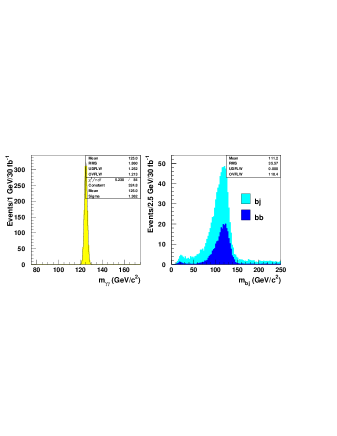
Subsequently, two mass window cuts are applied by requiring that:
-
•
GeV
-
•
GeV.
The photons and jets fulfilling these requirements are combined to form the invariant mass as shown in Figure 5. The mass resolution is improved down to a value of 5 GeV/ by constraining the reconstructed masses and to the light Higgs mass , as shown on the right-hand plot of Figure 5.
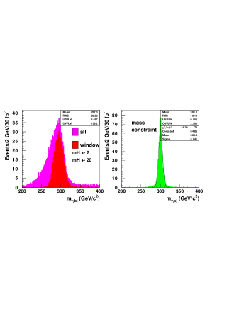
The signal acceptances after the various cuts described above are given in Table 1.
| Cuts | GeV/ | GeV/ |
|---|---|---|
| photons kinematics selection | 46% | 51% |
| jets kinematics selection | 36% | 28% |
| b-tagging | 76% | 78% |
| window cut | 83% | 85% |
| window cut | 49% | 53% |
| total | 5% | 5% |
The same analysis procedure is applied to the background sample. The resulting and distributions are shown in Figure 6.
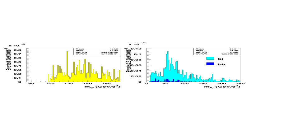
Since there are some uncertainties concerning the level of the background, a more conservative approach is also tried: the mass window cuts are loosened to keep events fulfilling:
-
•
GeV/
-
•
GeV/
The invariant mass distributions for this conservative approach are shown in Figure 7.
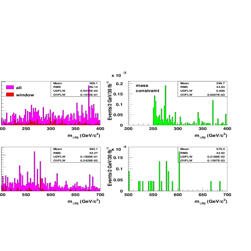
3.5 Results
The final number of events selected is obtained by counting the candidates after all cuts within a mass window of for signal and background. The results are shown in Table 2.
| GeV/ | GeV | ||
|---|---|---|---|
| background | 0 | background | 0 |
| background (conserv.) | background (conserv.) | 0 | |
| TeV | 380.1 | TeV | 575.8 |
| TeV | 3.8 | TeV | 5.9 |
| TeV | 680.4 | TeV | 439.9 |
| TeV | 5.5 | TeV | 5.9 |
Since this channel is practically background free, the usual significance is not relevant. A signal discovery, defined to be a minimum of ten events, is straightforward for low values of early in the physics program of the LHC. This is shown in Table 3 where the minimum integrated luminosities needed for discovery are shown. Approximately 1 is needed for TeV while requiring and .
In the special case where , the cross-section is proportional to . Therefore the maximum reach in is derived from this study. This is obtained using the prescription of [272]: for a known mean background of zero, the signal mean is larger than 10 with 95% CL if the number of observed events is larger than 18. The corresponding reach in is 4.6 TeV for GeV and 5.7 TeV for GeV.
4
The channel provides another potentially interesting signal for radion discovery, although the background is higher and the reconstructed mass resolutions are poorer than in the channel.
In order to provide a trigger, a leptonic decay of the is required. Here, only the case when one decays leptonically and the other hadronically is considered. As above, the events were generated by appropriately adapting the process of MSSM decay of the heavy Higgs into two light Higgs bosons (h) in Pythia 6.158 [113]. The effect of the ATLAS detector on the resolution and efficiency of reconstruction of these events was simulated with the ATLAS fast simulation package (ATLFAST 2.53). The efficiency for hadronic reconstruction is assumed to be 40%. For b-jet tagging, an efficiency of 60% is assumed, with a rejection factor of 10 for c jets and 100 for light jets [97].
4.1 Signals and backgrounds
As in the previous section, the radion mass values investigated are 300 and 600 GeV, while the Higgs mass is set to 125 GeV.
The fast simulated samples are:
-
•
with one decaying leptonically and the other hadronically (10 000 events)
-
•
with one W decaying leptonically and the other hadronically ( events)
-
•
with one decaying leptonically and the other hadronically ( events). Initial and final state radiation provide additional jets which can fake the signal.
-
•
inclusive W bosons decaying leptonically (2 events).
4.2 The selection
The study is performed assuming conditions of low luminosity () since, at high luminosity (), the reconstructed mass resolution is seriously compromised by pile-up effects. [97]. The events are selected if they satisfy the following criteria:
-
•
A lepton is required with GeV, (this lepton serves as a trigger).
-
•
The transverse mass is required to be GeV. This cut rejects background events containing W bosons.
-
•
The invariant mass is determined by combining the lepton with a tagged -jet having GeV/, (see Figure 9). If more than one jet is tagged as a tau-jet, the combination with the mass nearest to is chosen.
-
•
A pair of b-tagged jets with GeV/ and is required and their jet-jet mass reconstructed (see Figure 9). If more than two jets are tagged as b-jets, the pair having the invariant mass closest to the Higgs mass is chosen.
-
•
Cuts on the reconstructed mass and mass are applied:
GeV and GeV in the case of the 300 GeV radion, and GeV and GeV in the case of the 600 GeV radion.
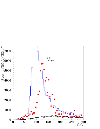
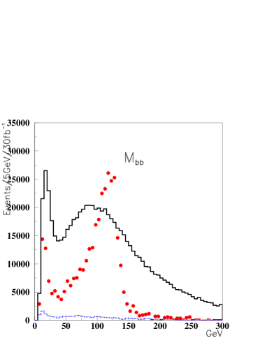
4.3 Results
Although the signal efficiency is low, the background rejection is high. The expected cross sections for signal and background before the event selection are given in Table 4 for TeV and . The branching ratios account for leptonic decays into a muon or an electron.
| Signal | = 300 GeV | = 600 GeV |
|---|---|---|
| 290 fb | 60 fb | |
| BR( hh) | 0.30 | 0.25 |
| BR(hh bb) | ||
| BR() | ||
| BR = | 3.98 fb | 0.652 fb |
| 180 pb | ||
| 40000 pb | ||
| 730 pb | ||
Figures 11 and 11 show the reconstructed masses for signal when =300 and 600 GeV respectively, for 30 fb-1, GeV and . The shape for a 300 GeV radion is similar to the one for background (mostly ), therefore systematic errors will most probably be dominated by the understanding of the level of this background.
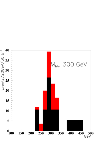

The expected number of events for an integrated luminosity of 30 (three years at low luminosity) are given in Table 5 for the two radion masses and for the backgrounds, when and 1 TeV.
| =300 GeV | =600 GeV | |
| Signal | 43 | 22 |
| 58 | ||
| 5.6 | 9.0 |
Requiring a minimum of 10 events and a , the maximum reach in is 1.05 and 1.4 TeV for =300 GeV and =600 GeV respectively, but the uncertainties in background subtraction may affect considerably the observability of this channel in the first case.
5 Conclusion
We have studied the possibility of observing the radion using the ATLAS detector at the LHC. The radion has couplings similar to those of the SM Higgs, and mixes with it, but it has also a large effective coupling to gluons. Re-interpreting results of previous studies on the search for a SM Higgs in ATLAS, a significance for observing a radion decaying into or has been determined as a function of its mass (see Figure 3). For an integrated luminosity of 100 , the values 10 (0.1) are obtained for the channel, with a mixing parameter =0 and a scale =1 (10)TeV, in the range . For the channel, 100 (1) for for the same conditions. Because the couplings are similar to those of the SM Higgs, a good measurement of the branching ratios will be necessary to discriminate between the two scalars.
The radion can also decay into a pair of Higgs scalars, if the masses permit. Two cases were examined: and , for radion masses of 300 and 600 GeV, for GeV and for an integrated luminosity of 30 fb-1. Limits on the maximal reach in were obtained for these two channels. For the channel, the background is negligible and the reach in is 4.6 (5.7) TeV for (600) GeV, when =0. For the channel, the similarity between the signal and background shapes make the observation of a radion of mass =300 GeV difficult, and the reach for is about 1.4 TeV for =600 GeV, when =0.
6 Acknowledgments
We warmly thank the organizers of Les Houches 2001. We thank T.Rizzo for useful discussions.
Part XVI Radion Mixing Effects on the Properties of the Standard Model
Higgs Boson
J.L.Hewett and T.G. Rizzo
The Randall-Sundrum(RS) model [4] offers a potential solution to the hierarchy problem that can be tested at present and future accelerators (for an overview of RS phenomenology, see [13, 283, 16]). In this model the SM fields lie on one of two branes that are embedded in 5-dimensional AdS space described by the metric , where is the 5-d curvature parameter of order the Planck scale. To solve the hierarchy problem the separation between the two branes, , must have a value of . That this quantity can be stabilized and made natural has been demonstrated by a number of authors [19, 284, 285, 286, 287, 288] and leads directly to the existence of a radion (), which corresponds to a quantum excitation of the brane separation. It can be shown that the radion couples to the trace of the stress-energy tensor with a strength of order the TeV scale, i.e., . (Note that in the notation of Ref. [13, 283, 16].) This leads to gauge and matter couplings that are qualitatively similar to those of the SM Higgs boson. The radion mass () is expected to be significantly below the scale implying that the radion may be the lightest new field predicted by the RS model. One may expect on general grounds that this mass should lie in the range of a few GeV . The phenomenology of the RS radion has been examined by a number of authors [276, 289, 290, 291, 292, 277, 293, 294, 295, 278] and in particular has been reviewed by Kribs [279].
On general grounds of covariance, the radion may mix with the SM Higgs field on the TeV brane through an interaction term of the form
| (1) |
where is the Higgs doublet field, is the Ricci scalar constructed out of the induced metric on the SM brane, and is a mixing parameter assumed to be of order unity and with unknown sign. The above action induces kinetic mixing between the ‘weak eigenstate’ and fields which can be removed through a set of field redefinitions and rotations. Clearly, since the radion and Higgs boson couplings to other SM fields differ this mixing will induce modifications in the usual SM expectations for the Higgs decay widths. To make unique predictions in this scenario we need to specify four parameters: the masses of the physical Higgs and radion fields, , the mixing parameter and the ratio , where is the vacuum expectation value of the SM Higgs GeV. Clearly the ratio cannot be too large as is already bounded from below by collider and electroweak precision data [13, 283, 16]; for definiteness we will take and in what follows although larger absolute values of have been entertained in the literature. The values of the two physical masses themselves are not arbitrary. When we require that the weak basis mass-squared parameters of the radion and Higgs fields be real, as is required by hermiticity, we obtain an additional constraint on the ratio of the physical radion and Higgs masses which only depends on the product . Explicitly one finds that either or where . This disfavors the radion having a mass too close to that of the Higgs when there is significant mixing; the resulting excluded region is shown in Fig. 1. These constraints are somewhat restrictive; if we take GeV and we find that either GeV or GeV. This lower mass range may be disfavored by direct searches.
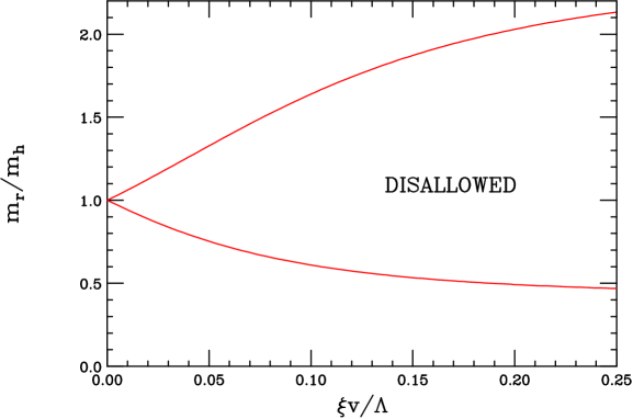
Following the notation of Giudice et al. [296], the coupling of the physical Higgs to the SM fermions and massive gauge bosons is now given by
| (2) |
where the angle is given above and can be calculated in terms of the parameters and and the physical Higgs and radion masses. Denoting the combinations and , the corresponding Higgs coupling to gluons can be written as with where is the -function and is a well-known kinematic function of the ratio of masses of the top quark to the physical Higgs. Similarly the physical Higgs couplings to two photons is now given by where , where and are the -functions and is another well-known kinematic function of the ratios of the and top masses to the physical Higgs mass. (Note that in the simultaneous limits we recover the usual SM results.) From these expressions we can now compute the change of the various decay widths and branching fractions of the SM Higgs due to mixing with the radion.
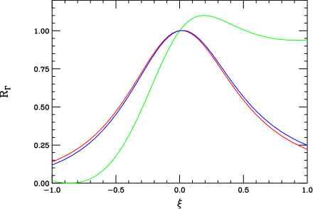
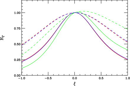
Fig. 2 shows the ratio of the various Higgs widths in comparison to their SM expectations as functions of the parameter assuming that GeV with different values of and . We see several features right away: () the shifts in the widths to and final states are very similar; this is due to the relatively large magnitude of while the combination is rather small. () On the other hand the shift for the final state is quite different since is smaller than and is quite large. () For relatively light radions with a low value of the width into the final state can come close to vanishing due to a strong destructive interference between the two contributions to the amplitude for values of near -1. () Increasing the value of has less of an effect on the width shifts than does a decrease in the ratio .
The deviation from the SM expectations for the various branching fractions, as well as the total width, of the Higgs are displayed in Fig. 3 as a function of the mixing parameter . We see that the gluon branching fraction and the total width may be drastically different than that of the SM. The former will affect the Higgs production cross section at the LHC. However, the , , and , where branching fractions receive small corrections to their SM values, of order for most of the parameter region. Observation of these shifts will require the accurate determination of the Higgs branching fractions available at an Linear Collider.
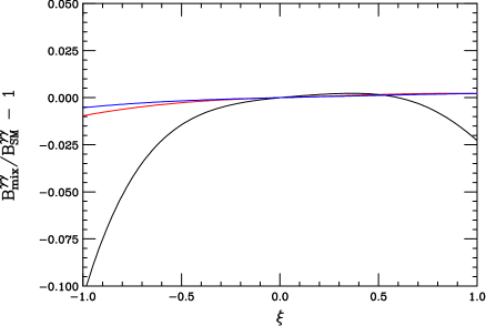
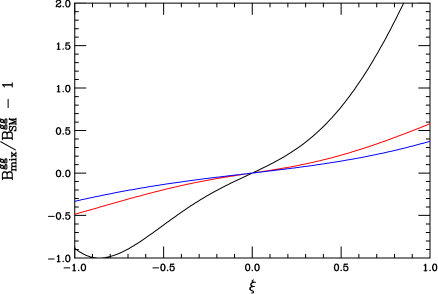
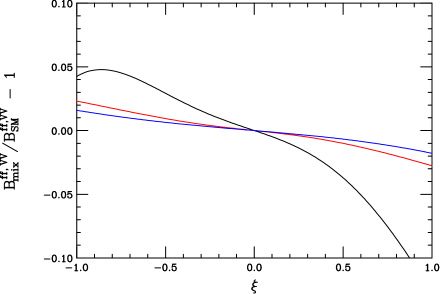
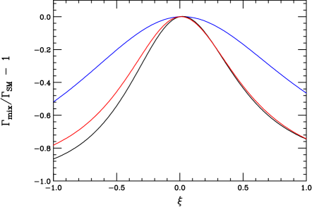
In summary, we see that Higgs-radion mixing, which is present in some extra dimensional scenarios, can have a substantial effect on the properties of the Higgs boson. These modifications affect the widths and branching fractions of Higgs decay into various final states, which in turn can alter the Higgs production cross section at the LHC and may require the precision of a Linear Collider to detect.
Part XVII Probing Universal Extra Dimensions at Present and Future Colliders
Thomas G. Rizzo
1 Introduction
The possibility that the gauge bosons of the Standard Model (SM) may be sensitive to the existence of extra dimensions near the TeV scale has been known for some time [20, 297, 298, 299, 300, 301, 302]. However, one finds that the phenomenology of these models is particularly sensitive to the manner in which the SM fermions (and Higgs bosons) are treated.
Perhaps the most democratic possibility requires all of the SM fields to propagate in the TeV-1 bulk [22], i.e., Universal Extra Dimensions (UED). In this case, the conservation of momentum in the extra dimensions is restored and one obtains interactions in the 4-d Lagrangian which take the form , which for flat space metrics vanishes unless , as a result of the afore mentioned momentum conservation. Although this momentum conservation is actually broken by orbifolding, one finds, at tree level, that KK number remains a conserved quantity. (As we will discuss below this conservation law is itself further broken at one loop order.) This implies that pairs of zero-mode fermions, which we identify with those of the SM, cannot directly interact singly with any of the excited modes in the gauge boson KK towers. Such a situation clearly limits any constraints arising from precision measurements since zero mode fermion fields can only interact with pairs of tower gauge boson fields. In addition, at colliders it now follows that KK states must be pair produced, thus significantly reducing the possible direct search reaches for these states. In fact, employing constraints from current experimental data, Appelquist, Cheng and Dobrescu (ACD) [22] find that the KK states in this scenario can be as light as GeV. If these states are, in fact, nearby, they will be copiously produced at the LHC, and possibly also at the Tevatron, in a variety of different channels. It is the purpose of this paper to estimate the production rates for pairs of these particles in various channels and to discuss their possible production signatures. This is made somewhat difficult by the apparent conservation of KK number which appears to forbid the decay of heavier excitations into lighter ones.
Now although the KK number is conserved at the tree level it becomes apparent that it is no longer so at loop order [303]. Consider a self-energy diagram with a field that has KK number of entering and a zero() mode leaving the graph; KK number conservation clearly does not forbid such an amplitude and constrains the 2 particles in the intermediate state to both have KK number ( and ). The existence of such amplitudes implies that all even and odd KK states mix separately so that the even KK excitations can clearly decay to zero modes while odd KK states can now decay down to the KK number=1 state. Thus it is KK parity, , which remains conserved while KK number itself is broken at one loop. Since the lightest KK excited states with have odd KK parity they remain stable unless new physics is introduced. As we are only concerned with the production of pairs of the lightest KK particles in our discussion below, we are faced with the possibility of producing heavy stable states at colliders.
2 Collider Production
Due to the conservation of KK parity, the first KK excitations of the SM fields must be pair-produced at colliders. At and lepton colliders the production cross sections for all the kinematically accessible KK states will very roughly be of order 100 fb which yields respectable event rates for luminosities in the range. A sample of relevant cross sections at both and colliders are shown in Fig. 1. In the case of collisions we have chosen the process as it the process which has the largest cross section for the production of the first KK state. Similarly, gauge boson pair production in collisions naturally leads to a large cross section. Clearly, such states once produced would not be easily missed for masses up to close the kinematic limit of the machine independently of how they decayed or if they were stable. To directly probe heavier masses we must turn to hadron colliders.
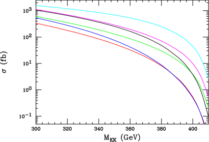
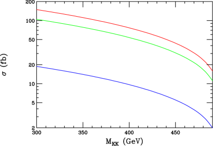
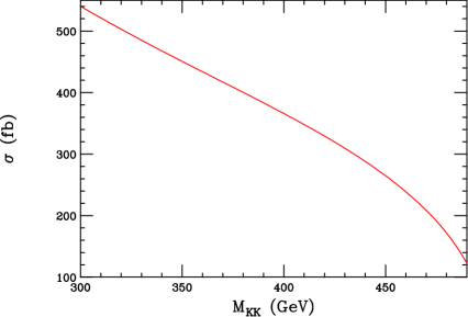
Since both QCD and electroweak exchanges can lead to KK pair production at hadron colliders there are three classes of basic processes to consider. Clearly the states with color quantum numbers will have the largest cross sections at hadron machines and there are a number of processes which can contribute to their production at order [304] several of which we list below:
| (1) |
where the primes are present to denote flavor differences. Fig. 2 shows the cross sections for these five processes at both the TeV Tevatron and the LHC summed over flavors. It is clear that during the Tevatron Run II we should expect a reasonable yield of these KK particles for masses below GeV if integrated luminosities in the range of 10-20 are obtained. Other processes that we have not considered may be able to slightly increase this reach. For larger masses we must turn to the LHC where we see that significant event rates should be obtainable for KK masses up to TeV or so for an integrated luminosity of 100 . As one might expect we see that the most important QCD processes for the production of KK states are different at the two colliders.
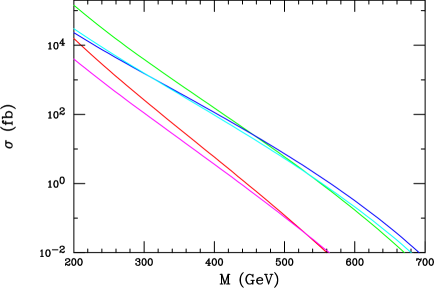
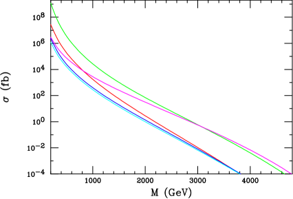
The real signature of the UED scenario is that all of the SM fields have KK excitations. Thus we will also want to observe the production of the SM color singlet states. Of course color singlet states can also be produced, with the largest cross sections being for associated production with a colored state at order ; these rates are of course smaller than for pairs of colored particles as can be seen in Fig. 3. Here we see reasonable rates are obtained for KK masses in excess of TeV or so. Lastly, it is possible to pair produce color singlets via electroweak interactions which thus lead to cross sections of order . Due to the large center of mass energy of the LHC these cross sections can also lead to respectable production rates for KK masses as great as TeV as can be seen from Fig. 4. It is clear from this analysis that the LHC will have a significant search reach for both colored and non-colored KK states provided that the production signatures are reasonably distinct.
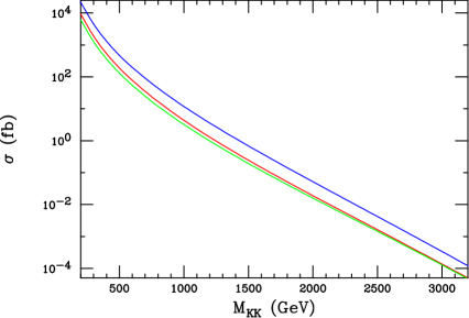
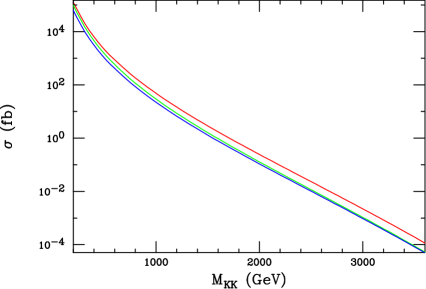
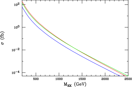
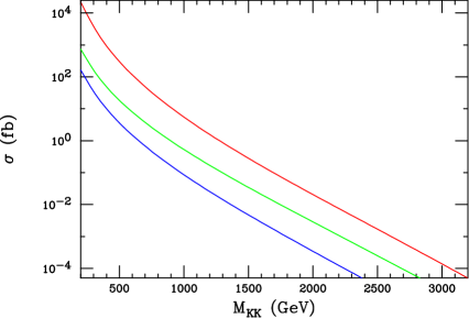
3 Signatures
When examining collider signatures for KK pair production in the UED there are two important questions to ask: () Are the lightest KK modes stable and () if they are unstable what are their decay modes? From the discussion above it is clear that without introducing any new physics the KK states are stable so we must consider this possibility when looking at production signatures.
In their paper ACD [22] argue that cosmological constraints possibly suggest that KK states in the TeV mass range must be unstable on cosmological time scales. (Of course this does not mean that they would appear unstable on the time scale of a collider experiment in which case our discussion is the same as that above.) This would require the introduction of new physics beyond that contained in the original UED model. There are several possible scenarios for such new physics. Here we will discuss three possibilities in what follows, the first two of which were briefly mentioned by ACD [22].
Scenario I: The TeV-1-scale UED model is embedded inside a thick brane in a higher -dimensional space, with a compactification scale , in which gravity is allowed to propagate in a manner similar to the model of Arkani-Hamed, Dimopoulos and Dvali [3, 12, 11]. Since the graviton wave functions are normalized on a torus of volume while the KK states are normalized over the overlap of a KK zero mode with any even or odd KK tower state and a graviton will be non-zero. In a sense, the brane develops a transition form-factor analogous to that described in [305]. This induces transitions of the form where represents the graviton field which appears as missing energy in the collider detector. This means that production of a pair of KK excitations of, e.g., quarks or gluons would appear as two jets plus missing energy in the detector; the corresponding production of a KK excited pair of gauge bosons would appear as the pair production of the corresponding zero modes together with missing energy. We can express this form-factor simply as
| (2) |
for even and odd KK states, respectively, where is the graviton mass. Here we have assumed that the thick brane resides at for all . Given these form-factors we can calculate the actual decay rate for , where we now must sum up the graviton towers by following the analyses in Ref. [296, 306]; this result should be relatively independent of the spin of the original KK state. Performing the necessary integrations numerically we obtain the results shown in Fig. 5.
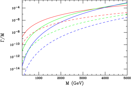
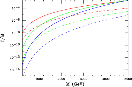
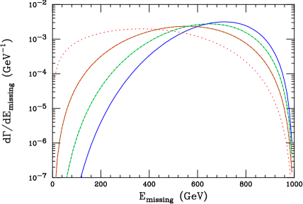
This figure shows that this mechanism provides for a very rapid decay over almost all of the parameter space. For light KK states with both and large the decay rate is suppressed and may lead to finite length charged tracks in the detector. (In particular the production of a charged KK state with a long lifetime would yield a kink-like track structure due to the decay to the graviton tower.) Although not a true two-body decay, Fig. 5 also shows that the typical missing energy in the gravitational decay of a KK state will be close to half its mass, which is quite significant for such heavy objects. It is clear that events with such a large fraction of missing energy should be observable above background given sufficient event rates. These events will not be confused with SUSY signals since they occur in every possible channel.
Scenario II: KK decays can be induced in the UED model by adding a ‘benign’ brane at some which induces new interactions. By ‘benign’ we mean that these new interactions only do what we need them to do and do not alter the basic properties of the UED model. The simplest form of such interactions are just the four dimensional variants of the terms in the the 5-d UED action. For example, one might add a term such as
| (3) |
where is some Yukawa-like coupling and is some large scale. Note that the brane is placed at some arbitrary position and not at the fixed points where only even KK modes would be effected. These new interactions result in a mixing of all KK states both even and odd and, in particular, with the zero mode. Thus we end up inducing decays of the form KK KK(0) KK(0). For KK fermions the decay into a fermion plus gauge boson zero mode is found to be given by
| (4) |
where is the induced mixing angle, is a color factor, , the relevant gauge coupling and PS is the phase space for the decay. It is assumed that the mixing angle is sufficiently small that single production of KK states at colliders remains highly suppressed but is large enough for the KK state to decay in the detector. For and a few this level of suppression is quite natural. (Numerically, it is clear that the KK state will decay inside the detector unless the mixing angle is very highly suppressed.) The resulting branching fractions can be found in Table 1 where we see numbers that are not too different than those for excited fermions in composite models with similar decay signatures. However, unlike excited SM fields, single production modes are highly suppressed. For KK excitations of the gauge bosons, their branching fractions into zero mode fermions will be identical to those of the corresponding SM fields apart from corrections due to phase space, i.e., the first excited KK state can decay to while the SM cannot.
| 0 | 41.0 | 14.4 | 44.6 | |
| 0 | 0 | 39.1 | 60.9 | |
| 89.8 | 2.3 | 2.1 | 5.7 | |
| 90.9 | 0.6 | 2.7 | 5.8 |
Scenario III: We can add a common bulk mass term to the fermion action, i.e., a term of the form , where and represent the 5-dimensional isodoublet and isosinglet SM fields. We chose a common mass both for simplicity and to avoid potentially dangerous flavor changing neutral currents. The largest influence of this new term is to modify the zero mode fermion wavefunction which is now no longer flat and takes the form and thus remains -even. Clearly there is now a significant overlap in the 5-d wavefunctions between pairs of fermion zero modes and any -even gauge KK mode which can be represented as another form-factor, , where . This form factor then describes the decay where represents a generic KK gauge field. Similarly we can obtain a form-factor that describes the corresponding decay which we denote by where is as above. It is clear that the decays of KK states in this scenario will be essentially identical to Scenario II above although they are generated by a completely different kind of physics. Fig. 6 shows the shape of these two form-factors as a function of the parameter . The natural question to ask at this point is ‘what is the value of relative to ?’. It seems natural to imagine that the bulk mass would be of order the compactification scale, the only natural scale in the action, which would imply that so that large form-factors would be obtained. While this scenario works extremely well for the decay of -even states it does not work at all for the case of -odd states.
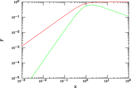
4 Summary and Conclusions
In this paper we have begun a detailed examination of the predictions of the Universal Extra Dimensions model for future colliders. Since indirect searches for such states give rather poor reaches, direct searches are of greater importance in this model. To obtain interesting search reaches requires a hadron collider such as the Tevatron or LHC. Based on counting events we expect the reach at the Tevatron Run II (LHC) for KK states to be GeV. Within the UED model itself these lightest KK states are stable even when loop corrections are included unless new interactions are introduced from elsewhere. If these states are indeed stable, the production of a large number of heavy stable charged particles would not be missed at either collider. It is more likely, however, that new physics does indeed enter, rendering the KK modes unstable. In this paper we have examined three new physics scenarios that induce finite KK lifetimes and compared their decay signatures.
Part XVIII Black Hole Production at Future Colliders
S. Dimopoulos and G. Landsberg
1 Introduction
An exciting consequence of TeV-scale quantum gravity [3, 11, 12] is the possibility of production of black holes (BHs) [307, 308, 309, 24, 23] at the LHC and beyond. This paper summarizes and extends our pioneer work on this subject [24] to the post-LHC future and discusses additional aspects of black-hole phenomenology left out from [24] due to lack of space. Since this work has been completed, numerous follow-up publications on this exciting subject have appeared in the archives, focusing on both the collider [40, 310, 30, 26] and cosmic ray [39, 38, 35] production. We hope that this new branch of phenomenology of extra dimensions will flourish in the months to come, as black hole production might be the very first evidence for the existence of large extra dimensions.
Black holes are well understood general-relativistic objects when their mass far exceeds the fundamental (higher dimensional) Planck mass TeV. As approaches , the BHs become “stringy” and their properties complex. In what follows, we will ignore this obstacle and estimate the properties of light BHs by simple semiclassical arguments, strictly valid for . We expect that this will be an adequate approximation, since the important experimental signatures rely on two simple qualitative properties: (i) the absence of small couplings and (ii) the “democratic” nature of BH decays, both of which may survive as average properties of the light descendants of BHs. Nevertheless, because of the unknown stringy corrections, our results are approximate estimates. For this reason, we will not attempt selective partial improvements – such as time dependence, angular momentum, charge, hair, and other higher-order general relativistic refinements – which, for light BHs, may be masked by larger unknown stringy effects. We will focus on the production and sudden decay of Schwarzschild black holes.
2 Production
The Schwarzschild radius of an -dimensional black hole is given by [311], assuming that extra dimensions are large ( ).
Consider two partons with the center-of-mass (c.o.m.) energy moving in opposite directions. Semiclassical reasoning suggests that if the impact parameter is less than the (higher dimensional) Schwarzschild radius, a BH with the mass forms. Therefore the total cross section can be estimated from geometrical arguments [312], and is of order
This expression contains no small coupling constants; if the parton c.o.m. energy reaches the fundamental Planck scale TeV then the cross section is of order TeV pb. At the LHC or VLHC, with the total c.o.m. energy TeV or 100-200 TeV, respectively, BHs will be produced copiously. To calculate total production cross section, we need to take into account that only a fraction of the total c.o.m. energy in a collision is achieved in a parton-parton scattering. We compute the full particle level cross section using the parton luminosity approach (see, e.g., Ref. [314]):
where the parton luminosity is defined as the sum over all the initial parton types:
and are the parton distribution functions (PDFs). We used the MRSD [315] PDF set with the scale taken to be equal to [316], which is within the allowed range for this PDF set, up to the VLHC kinematic limit. Cross section dependence on the choice of PDF is .
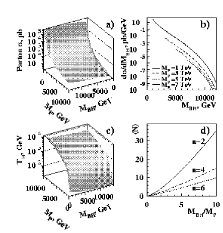
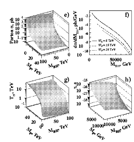
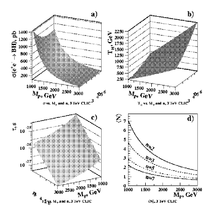
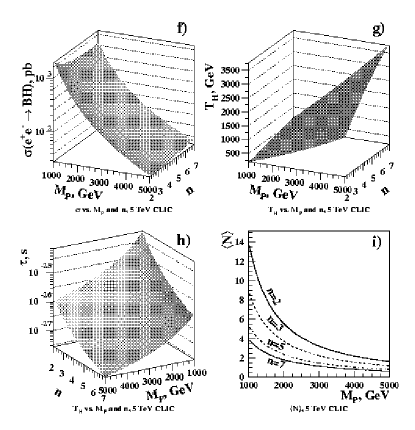


The differential cross sections for the BH produced at the LHC and a 200 TeV VLHC machines are shown in Figs. 1b and 1f, respectively, for several choices of . The total production cross section at the LHC for BH masses above ranges from 0.5 nb for TeV, to 120 fb for TeV and . If the fundamental Planck scale is TeV, the LHC, with the peak luminosity of 30 fb-1/year will produce over black holes per year. This is comparable to the total number of ’s produced at LEP, and suggests that we may do high precision studies of TeV BH physics, as long as the backgrounds are kept small. At the VLHC, BHs will be produced copiously for their masses and the value of the fundamental Planck scale as high as 25 TeV. The total production cross section is of the order of a millibarn for TeV and of order a picobarn for TeV.
Similarly, the black holes can be produced at future high-energy lepton colliders, such as CLIC or a muon collider. To a first approximation, such a machine produces black holes of a fixed mass, equal to the energy of the machine. The total cross section of such a BH produced at a 3 TeV and a 5 TeV machine, as a function of and , is shown in Fig 2a and Fig. 2f, respectively. For more elaborated studies of the BH production at electron colliders, one should take into account machine beamstrahlung. The beamstrahlung-corrected energy spectrum of the machine plays the same role as the parton luminosity at a hadron collider, except that for the machine it is peaked at the nominal machine energy, rather than at small values of , characteristic of a hadron collider. Using typical beamsstrahlung spectra expected for a 3 TeV or a 5 TeV CLIC machine, we show the differential cross section of the black hole production at a 3 and a 5 TeV CLIC in Fig. 2e and Fig. 2j, respectively.
3 Decay
The decay of the BH is governed by its Hawking temperature , which is proportional to the inverse radius, and given by [311]:
| (1) |
(see Figs. 1c,g and 2b,g). As the collision energy increases, the resulting BH gets heavier and its decay products get colder.
Note that the wavelength corresponding to the Hawking temperature is larger than the size of the black hole. Therefore, the BH acts as a point-radiator and emits mostly -waves. This indicates that it decays equally to a particle on the brane and in the bulk, since it is only sensitive to the radial coordinate and does not make use of the extra angular modes available in the bulk. Since there are many more particles on our brane than in the bulk, this has the crucial consequence that the BH decays visibly to standard model (SM) particles [309, 317].
The average multiplicity of particles produced in the process of BH evaporation is given by: , where is the energy spectrum of the decay products. In order to find , we note that the BH evaporation is a blackbody radiation process, with the energy flux per unit of time given by Planck’s formula: , where , and is a constant, which depends on the quantum statistics of the decay products ( for bosons, 1 for fermions, and 0 for Boltzmann statistics).
The spectrum of the BH decay products in the massless particle approximation is given by: . For averaging the multiplicity, we use the average of the distribution in the inverse particle energy:
| (2) |
where is a dimensionless constant that depends on the type of produced particles and numerically equals 0.68 for bosons, 0.46 for fermions, and for Boltzmann statistics. Since a mixture of fermions and bosons is produced in the BH decay, we can approximate the average by using Boltzmann statistics, which gives the following formula for the average multiplicity: . Using Eq. (1) for Hawking temperature, we obtain:
| (3) |
Eq. (3) holds for , i.e. ; otherwise, the Planck spectrum is truncated at by the decay kinematics [318]. The average number of particles produced in the process of BH evaporation is shown in Figs. 1d and 2d,i.
The lifetime of the BH can be estimated by using the Stefan’s law of thermal radiation. Since BH evaporation occurs primarily in three spatial dimensions, the canonical 3-dimensional Stefan’s law applies, and therefore the power dissipated by the Hawking’s radiation per unit area of the BH event horizon is , where is the Stefan-Boltzmann constant and is the Hawking temperature of the BH. Since the effective evaporation area of the BH is the area of a 3-dimensional sphere with the radius equal to the BH Schwarzschild radius , the total power dissipated by the BH is given by:
The BH lifetime is given by:
and using Eq. (1), as well as the expression for in natural units (), [319], we find:
The lifetime of a black hole as a function of its mass and the fundamental Planck scale is shown in Figs. 1h and 2c,h. A typical lifetime of a BH is s, which corresponds to a rather narrow width of the BH state GeV, i.e. typical for, e.g., a or resonance of a similar mass.
We emphasize that, throughout this paper, we ignore time evolution: as the BH decays, it gets lighter and hotter and its decay accelerates. We adopt the “sudden approximation” in which the BH decays, at its original temperature, into its decay products. This approximation should be reliable as the BH spends most of its time near its original mass and temperature, because that is when it evolves the slowest; furthermore, that is also when it emits the most particles. Later, when we test the Hawking’s mass-temperature relation by reconstructing Wien’s displacement law, we will minimize the sensitivity to the late and hot stages of the BHs life by looking at only the soft part of the decay spectrum. Proper treatment of time evolution, for , is difficult, since it immediately takes us to the stringy regime.
4 Branching Fractions
The decay of a BH is thermal: it obeys all local conservation laws, but otherwise does not discriminate between particle species (of the same mass and spin). Theories with quantum gravity near a TeV must have additional symmetries, beyond the standard , to guarantee proton longevity, approximate lepton number(s) and flavor conservation [320]. There are many possibilities: discrete or continuous symmetries, four dimensional or higher dimensional “bulk” symmetries [321]. Each of these possible symmetries constrains the decays of the black holes. Since the typical decay involves a large number of particles, we will ignore the constraints imposed by the few conservation laws and assume that the BH decays with roughly equal probability to all of the particles of the SM. Since there are six charged leptons and one photon, we expect of the particles to be hard, primary leptons and of the particles to be hard photons, each carrying hundreds of GeV of energy. This is a very clean signal, with negligible background, as the production of SM leptons or photons in high-multiplicity events at the LHC occurs at a much smaller rate than the BH production (see Fig. 3). These events are also easy to trigger on, since they contain at least one prompt lepton or photon with the energy above 100 GeV, as well as energetic jets.
5 Test of Hawking Radiation
Furthermore, since there are three neutrinos, we expect only average missing transverse energy () per event, which allows us to precisely estimate the BH mass from the visible decay products. We can also reconstruct the BH temperature by fitting the energy spectrum of the decay products to Planck’s formula. Simultaneous knowledge of the BH mass and its temperature allows for a test of the Hawking radiation and can provide evidence that the observed events come from the production of a BH, and not from some other new physics.
There are a few important experimental techniques that we will use to carry out the numerical test. First of all, to improve precision of the BH mass reconstruction we will use only the events with consistent with zero. Given the small probability for a BH to emit a neutrino or a graviton, total statistics won’t suffer appreciably from this requirement. Since BH decays have large jet activity, the resolution will be dominated by the jet energy resolution and the initial state radiation effects, and is expected to be GeV for a massive BH. Second, we will use only photons and electrons in the final state to reconstruct the Hawking temperature. The reason is twofold: final states with energetic electrons and photons have very low background at high , and the energy resolution for electrons and photons remains excellent even at the highest energies achieved in the process of BH evaporation. We do not use muons, as their momenta are determined by the track curvature in the magnetic field, and thus the resolution deteriorates fast with the muon momentum growth. We also ignore the -lepton decay modes, as the final states with ’s have much higher background than inclusive electron or photon final states, and also because their energies can not be reconstructed as well as those for the electromagnetic objects. The fraction of electrons and photons among the final state particles is only , but the vast amount of BHs produced at the LHC allows us to sacrifice the rest of the statistics to allow for a high-precision measurement. (Also, the large number of decay particles enhances the probability to have a photon or an electron in the event.) Finally, if the energy of a decay particle approaches the kinematic limit for pair production, , the shape of the energy spectrum depends on the details of the BH decay model. In order to eliminate this unwanted model dependence, we use only the low part of the energy spectrum with .
The experimental procedure is straightforward: we select the BH sample by requiring events with high mass ( TeV) and multiplicity of the final state (), which contain electrons or photons with energy GeV. We smear the energies of the decay products with the resolutions typical of the LHC detectors. We bin the events in the invariant mass with the bin size (500 GeV) much wider than the mass resolution. The mass spectrum of the BHs produced at the LHC with 100 fb-1 of integrated luminosity is shown in Fig. 3 for several values of and . Backgrounds from the SM jets and jets production, as estimated with PYTHIA [113], are small (see Fig. 3).
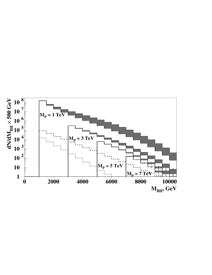
To determine the Hawking temperature as a function of the BH mass, we perform a maximum likelihood fit of the energy spectrum of electrons and photons in the BH events to Planck’s formula (with the coefficient determined by the particle spin), below the kinematic cutoff (/2). This fit is performed using the entire set of the BH events (i.e., not on the event-by-event basis), separately in each of the bins. We then use the measured vs. dependence and Eq. (1) to determine the fundamental Planck scale and the dimensionality of space . Note that to determine we can also take the logarithm of both sides of Eq. (1):
| (4) |
where the constant does not depend on the BH mass, but only on and on detailed properties of the bulk space, such as the shape of extra dimensions. Therefore, the slope of a straight-line fit to the vs. data offers a direct way of determining the dimensionality of space. This is a multidimensional analog of Wien’s displacement law. Note that Eq. (4) is fundamentally different from other ways of determining the dimensionality of space-time, e.g. by studying a monojet signature or virtual graviton exchange processes, also predicted by theories with large extra dimensions. (The properties of the latter two processes always depend on the volume of the extra-dimensional space, i.e. they cannot yield informaton on the number of extra dimensions without specific assumptions on their relative size.)
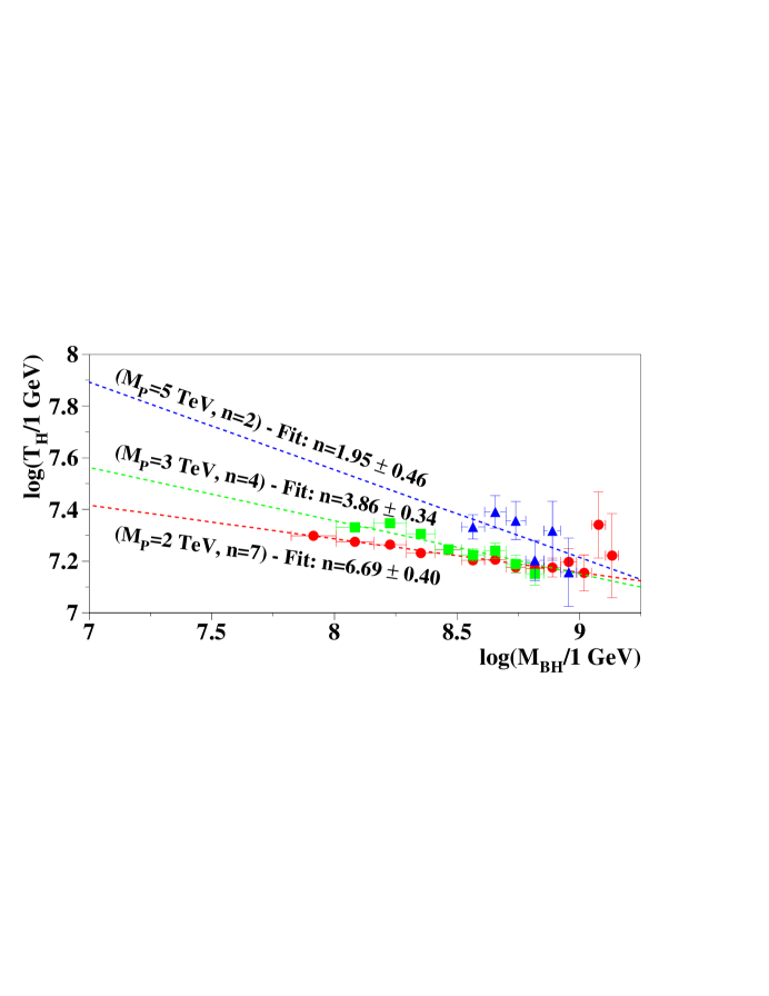
A test of Wien’s law at the LHC would provide a confirmation that the observed and event excess is due to BH production. It would also be the first experimental test of Hawking’s radiation hypothesis. Figure 4 shows typical fits to the simulated BH data at the LHC, corresponding to 100 fb-1 of integrated luminosity, for the highest fundamental Planck scales that still allow for determination of the dimensionality of space with reasonable precision. The reach of the LHC for the fundamental Planck scale and the number of extra dimensions via Hawking radiation extends to TeV and is summarized in Table 1 [322].
Similar tests can be performed at the VLHC and CLIC machines. While the VLHC case is identical to that at the LHC, with appropriately scaled energies, CLIC is complementary to the LHC in many ways, as the maximum number of BH produced at CLIC is found at the highest accessible masses. This has the advantage that the stringy effects, as well as the kinematic distortion of the Planck black-body spectrum, decrease with the increase of the BH mass. Thus the vs. fit at CLIC is less affected by these unknown effects. Preliminary studies show that statistical sensitivity to the number of extra dimensions and the value of the fundamental Planck scale at CLIC is similar to that at the LHC.
| 1 TeV | 2 TeV | 3 TeV | 4 TeV | 5 TeV | |
|---|---|---|---|---|---|
| 1%/0.01 | 1%/0.02 | 3.3%/0.10 | 16%/0.35 | 40%/0.46 | |
| 1%/0.01 | 1.4%/0.06 | 7.5%/0.22 | 30%/1.0 | 48%/1.2 | |
| 1%/0.01 | 2.3%/0.13 | 9.5%/0.34 | 35%/1.5 | 54%/2.0 | |
| 1%/0.02 | 3.2%/0.23 | 17%/1.1 | |||
| 1%/0.03 | 4.2%/0.34 | 23%/2.5 | Fit fails | ||
| 1%/0.07 | 4.5%/0.40 | 24%/3.8 | |||
Note, that the BH discovery potential at the LHC and VLHC is maximized in the channels, where background is much smaller than that in the channel (see Fig. 3). The reach of a simple counting experiment extends up to TeV at the LHC and TeV at the VLHC (–7), where one would expect to see a handful of BH events with negligible background.
6 Black Hole Monte Carlo Event Generator
A Monte Carlo package, TRUENOIR, has been developed for simulating production and decay of the black holes at high-energy colliders. This package is a plug-in module for the PYTHIA [113] Monte Carlo generator. It uses a heuristic algorithm and conservation of baryon and lepton numbers, as well as the QCD color, to simulate the decay of a black hole in a rapid-decay approximation. While the limitations of such a simplistic approach are clear, further improvements to this generator are being worked on. In the meantime, it provides a useful qualitative tool to study the detector effects and other aspects of the BH event reconstruction. Figure 5 shows a display of a typical BH event at a 5 TeV CLIC collider, produced using the TRUENOIR code. A characteristic feature of this event is extremely large final state multiplicity, very atypical of the events produced in collisions.
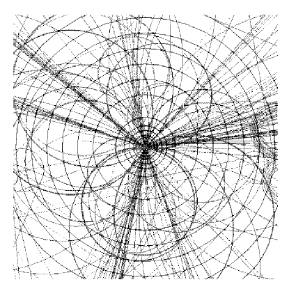
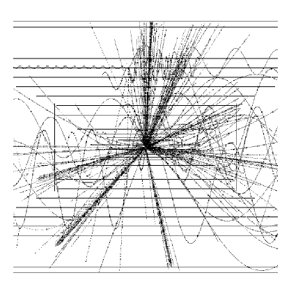
7 Summary
Black hole production at the LHC and beyond may be one of the early signatures of TeV-scale quantum gravity. It has three advantages:
-
•
(i) Large Cross Section: No small dimensionless coupling constants, analogous to , suppress the production of BHs. This leads to enormous rates.
-
•
(ii) Hard, Prompt, Charged Leptons and Photons: Thermal decays are flavor-blind. This signature has practically vanishing SM background.
-
•
(iii) Little Missing Energy: This facilitates the determination of the mass and the temperature of the black hole, and may lead to a test of Hawking radiation.
It is desirable to improve our primitive estimates, especially for the light black holes (); this will involve string theory. Nevertheless, the most telling signatures of BH production – large and growing cross sections; hard leptons, photons, and jets – emerge from qualitative features that are expected to be reliably estimated from the semiclassical arguments of this paper.
Perhaps black holes will be the first signal of TeV-scale quantum gravity. This depends on, among other factors, the relative magnitude of and the (smaller) string scale . For , the vibrational modes of the string may be the first indication of the new physics.
Studies of the BH properties at future facilities, including very high-energy lepton and hadron colliders, would make it possible to map out properties of large extra dimensions, to measure the effects of quantum gravity, and to provide insight into other quantum phenomena, such as Hawking radiation, the information paradox, etc.
8 Acknowledgments
We would like to thank Gia Dvali, Veronika Hubeny, Nemanja Kaloper, Elias Kiritsis, Joe Lykken, Konstantin Matchev, Steve Mrenna, and Lenny Susskind for valuable conversations. Many thanks to the organizers of the Les Houches workshop, where this work was started, for creating an excellent scientific atmosphere and productive environment. This work was partially supported by the U.S. DOE Grant No. DE-FG02-91ER40688, NSF Grant No. PHY-9870115, and A.P. Sloan Foundation.
References
- [1] N. Polonsky, Lect. Notes Phys. M68, 1 (2001), hep-ph/0108236.
- [2] C. T. Hill and E. H. Simmons, Strong dynamics and electroweak symmetry breaking (2002), hep-ph/0203079.
- [3] N. Arkani-Hamed, S. Dimopoulos, and G. R. Dvali, Phys. Lett. B429, 263 (1998), hep-ph/9803315.
- [4] L. Randall and R. Sundrum, Phys. Rev. Lett. 83, 3370 (1999), hep-ph/9905221.
- [5] B. C. Allanach et al., Eur. Phys. J. (2002), hep-ph/0202233.
- [6] J. L. Feng, K. T. Matchev, and T. Moroi, Phys. Rev. Lett. 84, 2322 (2000), hep-ph/9908309.
- [7] J. L. Feng and K. T. Matchev, Phys. Rev. D63, 095003 (2001), hep-ph/0011356.
- [8] S. F. King and M. Oliveira, Phys. Rev. D60, 035003 (1999), hep-ph/9804283.
- [9] B. Allanach et al., Searching for R-parity violation at Run-II of the Tevatron (1999), hep-ph/9906224.
- [10] J. A. Formaggio et al. (NuTeV), Phys. Rev. Lett. 84, 4043 (2000), hep-ex/9912062.
- [11] I. Antoniadis, N. Arkani-Hamed, S. Dimopoulos, and G. R. Dvali, Phys. Lett. B436, 257 (1998), hep-ph/9804398.
- [12] N. Arkani-Hamed, S. Dimopoulos, and G. R. Dvali, Phys. Rev. D59, 086004 (1999), hep-ph/9807344.
- [13] H. Davoudiasl, J. L. Hewett, and T. G. Rizzo, Phys. Rev. Lett. 84, 2080 (2000), hep-ph/9909255.
- [14] H. Davoudiasl, J. L. Hewett, and T. G. Rizzo, Phys. Lett. B473, 43 (2000), hep-ph/9911262.
- [15] A. Pomarol, Phys. Lett. B486, 153 (2000), hep-ph/9911294.
- [16] H. Davoudiasl, J. L. Hewett, and T. G. Rizzo, Phys. Rev. D63, 075004 (2001), hep-ph/0006041.
- [17] T. Gherghetta and A. Pomarol, Nucl. Phys. B586, 141 (2000), hep-ph/0003129.
- [18] J. L. Hewett, F. J. Petriello, and T. G. Rizzo, Precision measurements and fermion geography in the Randall-Sundrum model revisited (2002), hep-ph/0203091.
- [19] W. D. Goldberger and M. B. Wise, Phys. Rev. Lett. 83, 4922 (1999), hep-ph/9907447.
- [20] I. Antoniadis, Phys. Lett. B246, 377 (1990).
- [21] N. Arkani-Hamed and M. Schmaltz, Phys. Rev. D61, 033005 (2000), hep-ph/9903417.
- [22] T. Appelquist, H.-C. Cheng, and B. A. Dobrescu, Phys. Rev. D64, 035002 (2001), hep-ph/0012100.
- [23] S. B. Giddings and S. Thomas, Phys. Rev. D65, 056010 (2002), hep-ph/0106219.
- [24] S. Dimopoulos and G. Landsberg, Phys. Rev. Lett. 87, 161602 (2001), hep-ph/0106295.
- [25] S. B. Giddings, Black hole production in TeV-scale gravity, and the future of high energy physics (2001), hep-ph/0110127.
- [26] K. Cheung, Black hole production and large extra dimensions (2001), hep-ph/0110163.
- [27] G. Landsberg, Discovering new physics in the decays of black holes (2001), hep-ph/0112061.
- [28] S. Hofmann et al., Suppression of high-P(T) jets as a signal for large extra dimensions and new estimates of lifetimes for meta stable micro black holes: From the early universe to future colliders (2001), hep-ph/0111052.
- [29] D. M. Eardley and S. B. Giddings, Classical black hole production in high-energy collisions (2002), gr-qc/0201034.
- [30] S. Hossenfelder, S. Hofmann, M. Bleicher, and H. Stocker, Quasi-stable black holes at LHC (2001), hep-ph/0109085.
- [31] E.-J. Ahn, M. Cavaglia, and A. V. Olinto, Brane factories (2002), hep-th/0201042.
- [32] M. Kowalski, A. Ringwald, and H. Tu, Phys. Lett. B529, 1 (2002), hep-ph/0201139.
- [33] L. A. Anchordoqui, J. L. Feng, H. Goldberg, and A. D. Shapere, Black holes from cosmic rays: Probes of extra dimensions and new limits on TeV-scale gravity (2001), hep-ph/0112247.
- [34] Y. Uehara, Production and detection of black holes at neutrino array (2001), hep-ph/0110382.
- [35] R. Emparan, M. Masip, and R. Rattazzi, Phys. Rev. D65, 064023 (2002), hep-ph/0109287.
- [36] J. Alfaro and G. Palma, Loop quantum gravity corrections and cosmic rays decays (2001), hep-th/0111176.
- [37] D. Kazanas and A. Nicolaidis, Cosmic rays and large extra dimensions (2001), hep-ph/0109247.
- [38] L. Anchordoqui and H. Goldberg, Phys. Rev. D65, 047502 (2002), hep-ph/0109242.
- [39] J. L. Feng and A. D. Shapere, Phys. Rev. Lett. 88, 021303 (2002), hep-ph/0109106.
- [40] M. B. Voloshin, Phys. Lett. B518, 137 (2001), hep-ph/0107119.
- [41] M. B. Voloshin, Phys. Lett. B524, 376 (2002), hep-ph/0111099.
- [42] T. G. Rizzo, JHEP 02, 011 (2002), hep-ph/0201228.
- [43] H. P. Nilles, Phys. Lett. B115, 193 (1982).
- [44] H. P. Nilles, Nucl. Phys. B217, 366 (1983).
- [45] A. H. Chamseddine, R. Arnowitt, and P. Nath, Phys. Rev. Lett. 49, 970 (1982).
- [46] R. Barbieri, S. Ferrara, and C. A. Savoy, Phys. Lett. B119, 343 (1982).
- [47] H. P. Nilles, M. Srednicki, and D. Wyler, Phys. Lett. B120, 346 (1983).
- [48] E. Cremmer, P. Fayet, and L. Girardello, Phys. Lett. B122, 41 (1983).
- [49] S. Ferrara, L. Girardello, and H. P. Nilles, Phys. Lett. B125, 457 (1983).
- [50] L. J. Hall, J. Lykken, and S. Weinberg, Phys. Rev. D27, 2359 (1983).
- [51] S. K. Soni and H. A. Weldon, Phys. Lett. B126, 215 (1983).
- [52] P. Nath, R. Arnowitt, and A. H. Chamseddine, Nucl. Phys. B227, 121 (1983).
- [53] A. Dedes, A. B. Lahanas, and K. Tamvakis, Phys. Rev. D53, 3793 (1996), hep-ph/9504239.
- [54] A. Dedes, Radiative Breaking of Gauge Symmetries in the MSSM and in its Extensions (1998), hep-ph/9803339.
- [55] S. Heinemeyer, W. Hollik, and G. Weiglein, Comput. Phys. Commun. 124, 76 (2000), see also hep-ph/0002213. The codes are accessible via www.feynhiggs.de., hep-ph/9812320.
- [56] S. P. Martin and M. T. Vaughn, Phys. Lett. B318, 331 (1993), hep-ph/9308222.
- [57] H. Arason et al., Phys. Rev. D46, 3945 (1992).
- [58] D. M. Pierce, J. A. Bagger, K. Matchev, and R. jie Zhang, Nucl. Phys. B491, 3 (1997), hep-ph/9606211.
- [59] M. Drees and M. M. Nojiri, Phys. Rev. D45, 2482 (1992).
- [60] V. Barger, M. S. Berger, and P. Ohmann, Phys. Rev. D49, 4908 (1994), hep-ph/9311269.
- [61] S. P. Martin, Two-loop effective potential for a general renormalizable theory and softly broken supersymmetry (2001), hep-ph/0111209.
- [62] S. Heinemeyer, W. Hollik, and G. Weiglein, Phys. Rev. D58, 091701 (1998), hep-ph/9803277.
- [63] S. Heinemeyer, W. Hollik, and G. Weiglein, Phys. Lett. B440, 296 (1998), hep-ph/9807423.
- [64] S. Heinemeyer, W. Hollik, and G. Weiglein, Eur. Phys. J. C9, 343 (1999), hep-ph/9812472.
- [65] S. Ambrosanio, A. Dedes, S. Heinemeyer, S. Su, and G. Weiglein, Nucl. Phys. B624, 3 (2002), hep-ph/0106255.
- [66] A. Brignole, G. Degrassi, P. Slavich, and F. Zwirner, On the O(alpha**2(t)) two-loop corrections to the neutral Higgs boson masses in the MSSM (2001), hep-ph/0112177.
- [67] J. R. Espinosa and R.-J. Zhang, Nucl. Phys. B586, 3 (2000), hep-ph/0003246.
- [68] M. Frank, S. Heinemeyer, W. Hollik, and G. Weiglein, FeynHiggs1.2: Hybrid MS-bar / on-shell renormalization for the CP-even Higgs boson sector in the MSSM (2002), hep-ph/0202166.
- [69] A. Dedes, S. Heinemeyer, S. Su, and G. Weiglein, Soft SUSY-breaking scenarios in the light of Higgs searches at LEP2 (2001), hep-ph/0110219.
- [70] M. Battaglia et al., Post-LEP CMSSM benchmarks for supersymmetry (2001), hep-ph/0112013.
- [71] A. Dedes, K. Tamvakis, and A. B. Lahanas, Z observables and the effective weak mixing angle in the MSSM (1998), hep-ph/9805426.
- [72] B. C. Allanach, D. Grellscheid, and F. Quevedo, Selecting supersymmetric string scenarios from sparticle spectra (2001), hep-ph/0111057.
- [73] G. A. Blair, W. Porod, and P. M. Zerwas, Phys. Rev. D63, 017703 (2001), hep-ph/0007107.
- [74] B. C. Allanach, Comput. Phys. Commun. 143, 305 (2002), hep-ph/0104145.
- [75] S. Heinemeyer, W. Hollik, and G. Weiglein, Phys. Lett. B455, 179 (1999), hep-ph/9903404.
- [76] H. E. Haber, R. Hempfling, and A. H. Hoang, Z. Phys. C75, 539 (1997), hep-ph/9609331.
- [77] M. Battaglia et al., Eur. Phys. J. C22, 535 (2001), hep-ph/0106204.
- [78] B. C. Allanach, C. G. Lester, M. A. Parker, and B. R. Webber, JHEP 09, 004 (2000), hep-ph/0007009.
- [79] H. Abramowicz et al. (ATLAS), Technical Report CERN/LHCC 99-15 (1999).
- [80] H. Baer, F. E. Paige, S. D. Protopopescu, and X. Tata, ISAJET 7.48: A Monte Carlo event generator for p p, anti-p p, and e+ e- reactions (1999), hep-ph/0001086.
- [81] A. Djouadi et al. (MSSM Working Group), The minimal supersymmetric standard model: Group summary report (1998), hep-ph/9901246.
- [82] S. Moretti, Tools for supersymmetry (2001).
- [83] B. C. Allanach, Theoretical uncertainties in sparticle mass predictions (2001), hep-ph/0110227.
- [84] B. C. Allanach, J. P. J. Hetherington, M. A. Parker, and B. R. Webber, JHEP 08, 017 (2000), hep-ph/0005186.
- [85] J. A. Aguilar-Saavedra et al. (ECFA/DESY LC Physics Working Group), TESLA Technical Design Report Part III: Physics at an e+e- Linear Collider (2001), hep-ph/0106315.
- [86] G. W. Anderson and D. J. Castano, Phys. Lett. B347, 300 (1995), hep-ph/9409419.
- [87] R. Barbieri and G. F. Giudice, Nucl. Phys. B306, 63 (1988).
- [88] J. R. Ellis, J. S. Hagelin, D. V. Nanopoulos, K. A. Olive, and M. Srednicki, Nucl. Phys. B238, 453 (1984).
- [89] A. Gabutti, M. Olechowski, S. Cooper, S. Pokorski, and L. Stodolsky, Astropart. Phys. 6, 1 (1996), hep-ph/9602432.
- [90] H. Baer and M. Brhlik, Phys. Rev. D53, 597 (1996), hep-ph/9508321.
- [91] L. Alvarez-Gaume, J. Polchinski, and M. B. Wise, Nucl. Phys. B221, 495 (1983).
- [92] L. E. Ibanez, Phys. Lett. B118, 73 (1982).
- [93] J. R. Ellis, D. V. Nanopoulos, and K. Tamvakis, Phys. Lett. B121, 123 (1983).
- [94] K. Inoue, A. Kakuto, H. Komatsu, and S. Takeshita, Prog. Theor. Phys. 68, 927 (1982).
- [95] H. N. Brown et al. (Muon g-2), Phys. Rev. Lett. 86, 2227 (2001), hep-ex/0102017.
- [96] S. Abdullin et al. (CMS), J. Phys. G28, 469 (2002), hep-ph/9806366.
- [97] ATLAS Detector and Physics Performance Technical Design Report, CERN/LHCC/99-14, http://atlasinfo.cern.ch/Atlas/GROUPS/PHYSICS/TDR/access.html.
- [98] F. Paige and S. Protopopescu, in Supercollider Physics, p. 41, ed. D. Soper (World Scientific, 1986); H. Baer, F. Paige, S. Protopopescu and X. Tata, in Proceedings of the Workshop on Physics at Current Accelerators and Supercolliders, ed. J. Hewett, A. White and D. Zeppenfeld, (Argonne National Laboratory, 1993).
- [99] I. Hinchliffe, F. E. Paige, M. D. Shapiro, J. Soderqvist, and W. Yao, Phys. Rev. D55, 5520 (1997), hep-ph/9610544.
- [100] I. Hinchliffe and F. E. Paige, Phys. Rev. D60, 095002 (1999), hep-ph/9812233.
- [101] J. Bagger, J. L. Feng, and N. Polonsky, Nucl. Phys. B563, 3 (1999), hep-ph/9905292.
- [102] J. L. Feng, K. T. Matchev, and T. Moroi, Phys. Rev. D61, 075005 (2000), hep-ph/9909334.
- [103] LEPSUSY Working Group, Results of LEP about susy searches, http://lepsusy.web.cern.ch/lepsusy.
- [104] Results of Tevatron experiment about Susy search, http://www.physics.ucla.edu/ñachtman/269b/susy_tevatron.html and http://fnth37.fnal.gov/susy.html.
- [105] J. R. Ellis, D. V. Nanopoulos, and K. A. Olive, Phys. Lett. B508, 65 (2001), hep-ph/0102331.
- [106] J. R. Ellis and K. A. Olive, Phys. Lett. B514, 114 (2001), hep-ph/0105004.
- [107] CMS collaboration, CERN/LHCC/94-38 LHCCP1 (1994).
- [108] J. F. Gunion, Searching for low-energy supersymmetry (1998), hep-ph/9801417.
- [109] S. Abdullin and F. Charles, Nucl. Phys. B547, 60 (1999), hep-ph/9811402.
- [110] S. I. Bityukov and N. V. Krasnikov, The reach of LHC (CMS) for models with effective supersymmetry and nonuniversal gaugino masses (2000), hep-ph/0005246.
- [111] R.Brun et al., CERN DD/EE/84-1 (1986).
- [112] N. S.Abdullin, A.Khanov, CMS-TN/94-180 (1994).
- [113] T. Sjostrand, Comput. Phys. Commun. 82, 74 (1994).
- [114] CMS Collaboration, CMS TDR 1-5 (1997/1998).
- [115] U. Ellwanger, J. F. Gunion, and C. Hugonie, Establishing a no-lose theorem for NMSSM Higgs boson discovery at the LHC (2001), hep-ph/0111179.
- [116] J. F. Gunion, H. E. Haber, and T. Moroi, Will at least one of the Higgs bosons of the next-to- minimal supersymmetric extension of the standard model be observable at LEP2 or the LHC? (1996), hep-ph/9610337.
- [117] G. K. Yeghian, Upper bound on the lightest Higgs mass in supersymmetric theories (1999), hep-ph/9904488.
- [118] U. Ellwanger and C. Hugonie, Masses and couplings of the lightest Higgs bosons in the (M+1)SSM (1999), hep-ph/9909260.
- [119] J. Dai, J. F. Gunion, and R. Vega, Phys. Rev. Lett. 71, 2699 (1993), hep-ph/9306271.
- [120] E. Richter-Was and M. Sapinski, Acta Phys. Polon. B30, 1001 (1999).
- [121] M. Sapinski and D. Cavalli, Acta Phys. Polon. B32, 1317 (2001).
- [122] V. Drollinger, Finding H0 –¿ b anti-b at the LHC (2001), hep-ex/0105017.
- [123] D. Green, K. Maeshima, R. Vidal, W. Wu, CMS Note 2001/039 (2001).
- [124] We thank M. Sapinski for providing us with this extension, based on the same techniques as employed in the ATLAS analysis, as part of the Les Houches 2001 workshop.
- [125] D. Rainwater, D. Zeppenfeld, and K. Hagiwara, Phys. Rev. D59, 014037 (1999), hep-ph/9808468.
- [126] T. Plehn, D. Rainwater, and D. Zeppenfeld, Phys. Rev. D61, 093005 (2000), hep-ph/9911385.
- [127] D. Rainwater and D. Zeppenfeld, Phys. Rev. D60, 113004 (1999), hep-ph/9906218.
- [128] N. Kauer, T. Plehn, D. Rainwater, and D. Zeppenfeld, Phys. Lett. B503, 113 (2001), hep-ph/0012351.
- [129] D. Zeppenfeld, R. Kinnunen, A. Nikitenko, and E. Richter-Was, Phys. Rev. D62, 013009 (2000), hep-ph/0002036.
- [130] D. Zeppenfeld, contribution to Snowmass 2001 Proceedings.
- [131] J. F. Gunion, Hunting the Higgs boson(s) (2001), hep-ph/0106154.
- [132] U. Ellwanger, J. F. Gunion, C. Hugonie, work in progress.
- [133] LEP Higgs Working group, Note 2001-03 .
- [134] LEP Higgs Working group, Note 2001-04 .
- [135] J. R. Ellis, J. F. Gunion, H. E. Haber, L. Roszkowski, and F. Zwirner, Phys. Rev. D39, 844 (1989).
- [136] J. P. Derendinger and C. A. Savoy, Nucl. Phys. B237, 307 (1984).
- [137] M. Drees, Int. J. Mod. Phys. A4, 3635 (1989).
- [138] J. R. Espinosa and M. Quiros, Phys. Lett. B279, 92 (1992).
- [139] P. Binetruy and C. A. Savoy, Phys. Lett. B277, 453 (1992).
- [140] U. Ellwanger, M. Rausch de Traubenberg, and C. A. Savoy, Phys. Lett. B315, 331 (1993), hep-ph/9307322.
- [141] U. Ellwanger, M. Rausch de Traubenberg, and C. A. Savoy, Z. Phys. C67, 665 (1995), hep-ph/9502206.
- [142] U. Ellwanger, M. Rausch de Traubenberg, and C. A. Savoy, Nucl. Phys. B492, 21 (1997), hep-ph/9611251.
- [143] J.-i. Kamoshita, Y. Okada, and M. Tanaka, Phys. Lett. B328, 67 (1994), hep-ph/9402278.
- [144] F. Franke and H. Fraas, Phys. Lett. B353, 234 (1995), hep-ph/9504279.
- [145] S. F. King and P. L. White, Phys. Rev. D52, 4183 (1995), hep-ph/9505326.
- [146] S. F. King and P. L. White, Phys. Rev. D53, 4049 (1996), hep-ph/9508346.
- [147] S. W. Ham, S. K. Oh, and B. R. Kim, Phys. Lett. B414, 305 (1997), hep-ph/9612294.
- [148] N. V. Krasnikov, Mod. Phys. Lett. A13, 893 (1998), hep-ph/9709467.
- [149] A. Djouadi, M. Spira, and P. M. Zerwas, Z. Phys. C70, 427 (1996), hep-ph/9511344.
- [150] A. Djouadi, J. Kalinowski, and M. Spira, Comput. Phys. Commun. 108, 56 (1998), hep-ph/9704448.
- [151] R. Barate et al. (ALEPH), Phys. Lett. B495, 1 (2000), hep-ex/0011045.
- [152] P. Abreu et al. (DELPHI), Phys. Lett. B499, 23 (2001), hep-ex/0102036.
- [153] M. Acciarri et al. (L3), Phys. Lett. B508, 225 (2001), hep-ex/0012019.
- [154] G. Abbiendi et al. (OPAL), Phys. Lett. B499, 38 (2001), hep-ex/0101014.
- [155] T. Farris, J. F. Gunion, and H. E. Logan, Higgs sectors in which the only light Higgs boson is CP-odd and linear collider strategies for its discovery (2002), hep-ph/0202087.
- [156] A. Dedes and S. Moretti, Phys. Rev. Lett. 84, 22 (2000), hep-ph/9908516.
- [157] A. Dedes and S. Moretti, Nucl. Phys. B576, 29 (2000), hep-ph/9909418.
- [158] S. Y. Choi and J. S. Lee, Phys. Rev. D61, 115002 (2000), hep-ph/9910557.
- [159] E. Asakawa, S. Y. Choi, and J. S. Lee, Phys. Rev. D63, 015012 (2001), hep-ph/0005118.
- [160] A. G. Akeroyd and A. Arhrib, Phys. Rev. D64, 095018 (2001), hep-ph/0107040.
- [161] S. Y. Choi, K. Hagiwara, and J. S. Lee, Observability of the lightest MSSM Higgs boson with explicit CP violation via gluon fusion at the LHC (2001), hep-ph/0110138.
- [162] A. Arhrib, D. K. Ghosh, and O. C. W. Kong, Observing CP violating MSSM Higgs bosons at hadron colliders? (2001), hep-ph/0112039.
- [163] M. Dugan, B. Grinstein, and L. J. Hall, Nucl. Phys. B255, 413 (1985).
- [164] S. Dimopoulos and S. Thomas, Nucl. Phys. B465, 23 (1996), hep-ph/9510220.
- [165] T. Ibrahim and P. Nath, Phys. Rev. D57, 478 (1998), hep-ph/9708456.
- [166] T. Falk and K. A. Olive, Phys. Lett. B439, 71 (1998), hep-ph/9806236.
- [167] T. Ibrahim and P. Nath, Phys. Rev. D58, 111301 (1998), hep-ph/9807501.
- [168] M. Brhlik, G. J. Good, and G. L. Kane, Phys. Rev. D59, 115004 (1999), hep-ph/9810457.
- [169] A. Djouadi, J. L. Kneur, and G. Moultaka, Phys. Rev. Lett. 80, 1830 (1998), hep-ph/9711244.
- [170] A. Djouadi, J. L. Kneur, and G. Moultaka, Nucl. Phys. B569, 53 (2000), hep-ph/9903218.
- [171] A. Dedes and S. Moretti, Phys. Rev. D60, 015007 (1999), hep-ph/9812328.
- [172] A. Dedes and S. Moretti, Eur. Phys. J. C10, 515 (1999), hep-ph/9904491.
- [173] G. Belanger, F. Boudjema, and K. Sridhar, Nucl. Phys. B568, 3 (2000), hep-ph/9904348.
- [174] A. Dedes and S. Moretti, Higgs boson production in association with squark pairs in the MSSM at the LHC (1999), hep-ph/9909526.
- [175] A. Djouadi et al., The Higgs working group: Summary report (2000), hep-ph/0002258.
- [176] See, e.g.: http://www.cern.ch/LEPHIGGS/.
- [177] D. Stuart, talk given at ’XIth Recontres de Blois: Frontiers of Matter’, Blois, France, June–July 1999; P. Rebecchi, ibidem.
- [178] D. Chang, W.-Y. Keung, and A. Pilaftsis, Phys. Rev. Lett. 82, 900 (1999), hep-ph/9811202.
- [179] A. Pilaftsis, Phys. Lett. B471, 174 (1999), hep-ph/9909485.
- [180] D. A. Demir, Phys. Rev. D60, 055006 (1999), hep-ph/9901389.
- [181] D. A. Demir, Phys. Rev. D60, 095007 (1999), hep-ph/9905571.
- [182] A. Pilaftsis, Phys. Lett. B435, 88 (1998), hep-ph/9805373.
- [183] A. Pilaftsis, Phys. Rev. D58, 096010 (1998), hep-ph/9803297.
- [184] A. Pilaftsis and C. E. M. Wagner, Nucl. Phys. B553, 3 (1999), hep-ph/9902371.
- [185] M. Carena, J. R. Ellis, A. Pilaftsis, and C. E. M. Wagner, Nucl. Phys. B586, 92 (2000), hep-ph/0003180.
- [186] P. G. Harris et al., Phys. Rev. Lett. 82, 904 (1999).
- [187] E. D. Commins, S. B. Ross, D. DeMille, and B. C. Regan, Phys. Rev. A50, 2960 (1994).
- [188] Z. Kunszt, Nucl. Phys. B247, 339 (1984).
- [189] W. J. Marciano and F. E. Paige, Phys. Rev. Lett. 66, 2433 (1991).
- [190] H. L. Lai et al., Phys. Rev. D55, 1280 (1997), hep-ph/9606399.
- [191] T. Blazek and S. F. King, Phys. Lett. B518, 109 (2001), hep-ph/0105005.
- [192] J. R. Ellis, K. Enqvist, and D. V. Nanopoulos, Phys. Lett. B147, 99 (1984).
- [193] J. R. Ellis, K. Enqvist, and D. V. Nanopoulos, Phys. Lett. B151, 357 (1985).
- [194] G. F. Giudice and R. Rattazzi, Phys. Rept. 322, 419 (1999), hep-ph/9801271.
- [195] S. L. Dubovsky, D. S. Gorbunov, and S. V. Troitsky, Phys. Usp. 42, 623 (1999), hep-ph/9905466.
- [196] E. Cremmer, S. Ferrara, L. Girardello, and A. Van Proeyen, Nucl. Phys. B212, 413 (1983).
- [197] A. Brignole, F. Feruglio, and F. Zwirner, Nucl. Phys. B501, 332 (1997), hep-ph/9703286.
- [198] E. Perazzi, G. Ridolfi, and F. Zwirner, Nucl. Phys. B574, 3 (2000), hep-ph/0001025.
- [199] E. Perazzi, G. Ridolfi, and F. Zwirner, Nucl. Phys. B590, 287 (2000), hep-ph/0005076.
- [200] D. S. Gorbunov and A. V. Semenov, CompHEP package with light gravitino and sgoldstinos (2001), hep-ph/0111291.
- [201] D. A. Dicus and P. Roy, Phys. Rev. D42, 938 (1990).
- [202] D. S. Gorbunov, Nucl. Phys. B602, 213 (2001), hep-ph/0007325.
- [203] A. Brignole and A. Rossi, Nucl. Phys. B587, 3 (2000), hep-ph/0006036.
- [204] D. S. Gorbunov and V. A. Rubakov, Phys. Rev. D64, 054008 (2001), hep-ph/0012033.
- [205] D. Gorbunov, V. Ilyin, and B. Mele, Phys. Lett. B502, 181 (2001), hep-ph/0012150.
- [206] M. Nowakowski and S. D. Rindani, Phys. Lett. B348, 115 (1995), hep-ph/9410262.
- [207] J. A. Grifols, R. N. Mohapatra, and A. Riotto, Phys. Lett. B400, 124 (1997), hep-ph/9612253.
- [208] T. Gherghetta, Phys. Lett. B423, 311 (1998), hep-ph/9712343.
- [209] A. Pukhov et al., CompHEP: A package for evaluation of Feynman diagrams and integration over multi-particle phase space. User’s manual for version 33 (1999), hep-ph/9908288.
- [210] T. Adams et al. (NuTeV), Int. J. Mod. Phys. A16S1B, 761 (2001), hep-ex/0009007.
- [211] T. Adams et al. (NuTeV), Phys. Rev. Lett. 87, 041801 (2001), hep-ex/0104037.
- [212] A. Dedes, H. Dreiner, and P. Richardson, Phys. Rev. D65, 015001 (2002), hep-ph/0106199.
- [213] B. C. Allanach, A. Dedes, and H. K. Dreiner, Phys. Rev. D60, 075014 (1999), hep-ph/9906209.
- [214] K. Cheung and G. Landsberg, Kaluza-Klein states of the standard model gauge bosons: Constraints from high energy experiments (2001), hep-ph/0110346.
- [215] J. D. Lykken, Phys. Rev. D54, 3693 (1996), hep-th/9603133.
- [216] G. Shiu and S. H. H. Tye, Phys. Rev. D58, 106007 (1998), hep-th/9805157.
- [217] I. Antoniadis and C. Bachas, Phys. Lett. B450, 83 (1999), hep-th/9812093.
- [218] K. R. Dienes, E. Dudas, and T. Gherghetta, Nucl. Phys. B537, 47 (1999), hep-ph/9806292.
- [219] A. Pomarol and M. Quirós, Phys. Lett. B438, 255 (1998), hep-ph/9806263.
- [220] M. Masip and A. Pomarol, Phys. Rev. D60, 096005 (1999), hep-ph/9902467.
- [221] I. Antoniadis, K. Benakli, and M. Quirós, Phys. Lett. B460, 176 (1999), hep-ph/9905311.
- [222] P. Nath and M. Yamaguchi, Phys. Rev. D60, 116006 (1999), hep-ph/9903298.
- [223] P. Nath, Y. Yamada, and M. Yamaguchi, Phys. Lett. B466, 100 (1999), hep-ph/9905415.
- [224] T. G. Rizzo and J. D. Wells, Phys. Rev. D61, 016007 (2000), hep-ph/9906234.
- [225] R. Casalbuoni, S. De Curtis, D. Dominici, and R. Gatto, Phys. Lett. B462, 48 (1999), hep-ph/9907355.
- [226] A. Strumia, Phys. Lett. B466, 107 (1999), hep-ph/9906266.
- [227] C. D. Carone, Phys. Rev. D61, 015008 (2000), hep-ph/9907362.
- [228] A. Delgado, A. Pomarol, and M. Quirós, JHEP 01, 030 (2000), hep-ph/9911252.
- [229] F. Cornet, M. Relaño, and J. Rico, Phys. Rev. D61, 037701 (2000), hep-ph/9908299.
- [230] T. G. Rizzo, Phys. Rev. D61, 055005 (2000), hep-ph/9909232.
- [231] H. L. Lai et al. (CTEQ), Eur. Phys. J. C12, 375 (2000), hep-ph/9903282.
- [232] J. Breitweg et al. (ZEUS), Eur. Phys. J. C11, 427 (1999), hep-ex/9905032.
- [233] J. Breitweg et al. (ZEUS), Eur. Phys. J. C12, 411 (2000), hep-ex/9907010.
- [234] C. Adloff et al. (H1), Eur. Phys. J. C13, 609 (2000), hep-ex/9908059.
- [235] C. Adloff et al. (H1), Eur. Phys. J. C19, 269 (2001), hep-ex/0012052.
- [236] F. Abe et al. (CDF), Phys. Rev. Lett. 79, 2198 (1997).
- [237] B. Abbott et al. (DO Collaboration), Phys. Rev. Lett. 82, 4769 (1999), hep-ex/9812010.
- [238] LEP Electroweak Working Group, hep-ex/0103048 (2001).
- [239] R. Barate et al. (ALEPH Collaboration), Eur. Phys. J. C12, 183 (2000), hep-ex/9904011.
- [240] M. N. Minard and I. Tomalin (ALEPH), Fermion pair production in e+ e- collisions at 189-GeV and limits on physics beyond the standard model (1999), prepared for International Europhysics Conference on High- Energy Physics (EPS-HEP 99), Tampere, Finland, 15-21 Jul 1999.
- [241] R. Barate et al. (ALEPH Collaboration), ALEPH-2000-047; http://alephwww.cern.ch/ALPUB/oldconf/osaka00/fermion/osaka_final.ps.
- [242] R. Barate et al. (ALEPH Collaboration), ALEPH-2001-019; Http://alephwww.cern.ch/ALPUB/oldconf/oldconf01/24/fermion.ps.
- [243] P. Abreu et al. (DELPHI Collaboration), Eur. Phys. J. C11, 383 (1999).
- [244] P. Abreu et al. (DELPHI Collaboration), Phys. Lett. B485, 45 (2000), hep-ex/0103025.
- [245] P. Abreu et al. (DELPHI Collaboration), DELPHI-99-135; http://delphiwww.cern.ch/ pubxx/www/delsec/conferences /tampere99/paper_6_362.ps.gz.
- [246] P. Abreu et al. (DELPHI Collaboration), DELPHI-2000-128; http://delphiwww.cern.ch/ pubxx/www/delsec/delnote/public/2000_128_conf_427.ps.gz.
- [247] M. Acciarri et al. (L3 Collaboration), Phys. Lett. B370, 195 (1996).
- [248] M. Acciarri et al. (L3 Collaboration), Phys. Lett. B407, 361 (1997).
- [249] M. Acciarri et al. (L3 Collaboration), http://l3www.cern.ch/conferences/EPS99/papers/note_2398.ps.
- [250] M. Acciarri et al. (L3 Collaboration), Phys. Lett. B479, 101 (2000), hep-ex/0002034.
- [251] K. Ackerstaff et al. (OPAL Collaboration), Eur. Phys. J. C2, 441 (1998), hep-ex/9708024.
- [252] G. Abbiendi et al. (OPAL Collaboration), Eur. Phys. J. C6, 1 (1999), hep-ex/9808023.
- [253] G. Abbiendi et al. (OPAL Collaboration), Eur. Phys. J. C13, 553 (2000), hep-ex/9908008.
- [254] G. Abbiendi et al. (OPAL Collaboration), OPAL Note PN424; http://opal.web.cern.ch/Opal/pubs/physnote/html/pn424.html.
- [255] F. Abe et al. (CDF Collaboration), Phys. Rev. Lett. 77, 5336 (1996), erratum ibid. 78, 4307 (1997), hep-ex/9609011.
- [256] T. Affolder et al. (CDF Collaboration), Phys. Rev. D61, 091101 (2000), hep-ex/9912022.
- [257] B. Abbott et al. (DO Collaboration), Phys. Rev. Lett. 80, 666 (1998), hep-ex/9707016.
- [258] B. Abbott et al. (DO Collaboration), Phys. Rev. Lett. 82, 2457 (1999), hep-ex/9807014.
- [259] J. Lykken and S. Nandi, Phys. Lett. B485, 224 (2000), hep-ph/9908505.
- [260] E. L. Berger and H. Contopanagos, Phys. Rev. D54, 3085 (1996), hep-ph/9603326.
- [261] S. Catani, M. L. Mangano, P. Nason, and L. Trentadue, Phys. Lett. B378, 329 (1996), hep-ph/9602208.
- [262] S. Blusk (CDF Collaboration), in Proc. 30th International Conf. on High Energy Physics, ICHEP2000, Osaka, Japan, 27 July - 2 August 2000, edited by C.S. Lim, T. Yamanaka.
- [263] D. Chakraborty (DO Collaboration), in Proc. 30th International Conf. on High Energy Physics, ICHEP2000, Osaka, Japan, 27 July - 2 August 2000, edited by C.S. Lim, T. Yamanaka.
- [264] K. Cheung and G. Landsberg, Phys. Rev. D62, 076003 (2000), hep-ph/9909218.
- [265] R. Hamberg, W. L. van Neerven, and T. Matsuura, Nucl. Phys. B359, 343 (1991).
- [266] P. Nath and M. Yamaguchi, Phys. Rev. D60, 116004 (1999), hep-ph/9902323.
- [267] K. Cheung and G. Landsberg, in present proceedings (2002).
- [268] We warmly thank Tom Rizzo for providing us with the FORTRAN code for excitations production and for the help in implementing it.
- [269] D. F. E. Richter-Was and L. Poggioli, ATLFAST 2.0: a fast simulation package for ATLAS, aTLAS Internal Note ATL-PHYS-98-131, 1998.
- [270] J. C. Collins and D. E. Soper, Phys. Rev. D16, 2219 (1977).
- [271] D. Choudhury, R. Godbole, G. Polesello, in preparation.
- [272] G. J. Feldman and R. D. Cousins, Phys. Rev. D57, 3873 (1998), physics/9711021.
- [273] U. Baur, O. Brein, W. Hollik, C. Schappacher, and D. Wackeroth, Phys. Rev. D65, 033007 (2002), hep-ph/0108274.
- [274] T. G. Rizzo, Distinguishing Kaluza-Klein resonances from a Z’ in Drell- Yan processes at the LHC (2001), hep-ph/0109179.
- [275] B. C. Allanach, K. Odagiri, M. A. Parker, and B. R. Webber, JHEP 09, 019 (2000), hep-ph/0006114.
- [276] G. F. Giudice, R. Rattazzi, and J. D. Wells, Nucl. Phys. B595, 250 (2001), hep-ph/0002178.
- [277] S. B. Bae, P. Ko, H. S. Lee, and J. Lee, Phys. Lett. B487, 299 (2000), hep-ph/0002224.
- [278] K. Cheung, Phys. Rev. D63, 056007 (2001), hep-ph/0009232.
- [279] G. D. Kribs, Physics of the radion in the Randall-Sundrum scenario (2001), hep-ph/0110242.
- [280] J. L. Hewett and T. G. Rizzo, Radion mixing effects on the properties of the standard model Higgs boson (2002), hep-ph/0112343.
- [281] E. R.-W. et al., ATLAS Internal Note ATL-PHYS-96-074 (1996).
- [282] T. Sjostrand, private communication.
- [283] H. Davoudiasl, J. L. Hewett, and T. G. Rizzo, Phys. Lett. B493, 135 (2000), hep-ph/0006097.
- [284] W. D. Goldberger and M. B. Wise, Phys. Lett. B475, 275 (2000), hep-ph/9911457.
- [285] C. Csaki, M. Graesser, L. Randall, and J. Terning, Phys. Rev. D62, 045015 (2000), hep-ph/9911406.
- [286] C. Csaki, M. L. Graesser, and G. D. Kribs, Phys. Rev. D63, 065002 (2001), hep-th/0008151.
- [287] C. Charmousis, R. Gregory, and V. A. Rubakov, Phys. Rev. D62, 067505 (2000), hep-th/9912160.
- [288] T. Tanaka and X. Montes, Nucl. Phys. B582, 259 (2000), hep-th/0001092.
- [289] U. Mahanta and A. Datta, Phys. Lett. B483, 196 (2000), hep-ph/0002183.
- [290] T. Han, G. D. Kribs, and B. McElrath, Phys. Rev. D64, 076003 (2001), hep-ph/0104074.
- [291] M. Chaichian, A. Datta, K. Huitu, and Z.-h. Yu, Phys. Lett. B524, 161 (2002), hep-ph/0110035.
- [292] M. Chaichian, K. Huitu, A. Kobakhidze, and Z. H. Yu, Phys. Lett. B515, 65 (2001), hep-ph/0106077.
- [293] S. Bae and H. S. Lee, Phys. Lett. B506, 147 (2001), hep-ph/0011275.
- [294] S. C. Park, H. S. Song, and J. Song, Z boson pair production at LHC in a stabilized Randall- Sundrum scenario (2001), hep-ph/0103308.
- [295] S. R. Choudhury, A. S. Cornell, and G. C. Joshi, Radion signature in gamma gamma scattering (2000), hep-ph/0012043.
- [296] G. F. Giudice, R. Rattazzi, and J. D. Wells, Nucl. Phys. B544, 3 (1999), and revised version 2, e-print hep-ph/9811291, hep-ph/9811291.
- [297] I. Antoniadis, C. Munoz, and M. Quiros, Nucl. Phys. B397, 515 (1993), hep-ph/9211309.
- [298] I. Antoniadis and K. Benakli, Phys. Lett. B326, 69 (1994), hep-th/9310151.
- [299] I. Antoniadis and K. Benakli, Int. J. Mod. Phys. A15, 4237 (2000), hep-ph/0007226.
- [300] I. Antoniadis, K. Benakli, and M. Quiros, Phys. Lett. B331, 313 (1994), hep-ph/9403290.
- [301] K. Benakli, Phys. Lett. B386, 106 (1996), hep-th/9509115.
- [302] E. Accomando, I. Antoniadis, and K. Benakli, Nucl. Phys. B579, 3 (2000), hep-ph/9912287.
- [303] The author (T.R.) would like to thank A. Strumia for this important observation.
- [304] D. A. Dicus, C. D. McMullen, and S. Nandi, Collider implications of Kaluza-Klein excitations of the gluons (2000), hep-ph/0012259.
- [305] A. De Rujula, A. Donini, M. B. Gavela, and S. Rigolin, Phys. Lett. B482, 195 (2000), hep-ph/0001335.
- [306] T. Han, J. D. Lykken, and R.-J. Zhang, Phys. Rev. D59, 105006 (1999), and revised version 4, e-print hep-ph/9811350, hep-ph/9811350.
- [307] P. C. Argyres, S. Dimopoulos, and J. March-Russell, Phys. Lett. B441, 96 (1998), hep-th/9808138.
- [308] T. Banks and W. Fischler, hep-th/9906038 (1999).
- [309] R. Emparan, G. T. Horowitz, and R. C. Myers, Phys. Rev. Lett. 85, 499 (2000), hep-th/0003118.
- [310] S. Dimopoulos and R. Emparan, String balls at the LHC and beyond (2001), hep-ph/0108060.
- [311] R. C. Myers and M. J. Perry, Ann. Phys. 172, 304 (1986).
- [312] In fact the cross section is somewhat enhanced by initial-state attraction [309].
- [313] Exponential suppression of the BH production, claimed in [40] is not applicable to this work, as the BH collapse is due to a classical evolution, rather than tunneling. This was confirmed by, e.g., the analysis in Ref. [310].
- [314] E. Eichten, I. Hinchliffe, K. D. Lane, and C. Quigg, Rev. Mod. Phys. 56, 579 (1984).
- [315] A. D. Martin, W. J. Stirling, and R. G. Roberts, Phys. Lett. B306, 145 (1993).
- [316] While another choice of , as used, e.g., in [23], is also a logical possibility, we choose to use a more conservative assumption, as the actual relevant scale depends on unknown stringy effects, and likely to be somewhere between these two extremes.
- [317] L. Susskind, private communication.
- [318] To avoid this limitation when performing numerical tests of Wien’s law, we truncate the integrals in Eq. (2) at the kinematic limit (/2).
- [319] In the above calculatons we used the Stefan-Boltzmann constant, which is strictly speaking correct only for an evaporation via massless bosons. However, since the nature of our calculations is very approximate, this is a reasonable assumption.
- [320] Any form of new physics at a TeV requires such new symmetries (e.g., R-parity for TeV-scale SUSY).
- [321] N. Arkani-Hamed and S. Dimopoulos, Phys. Rev. D65, 052003 (2002), hep-ph/9811353.
- [322] We checked the effect of introducing an additional cutoff at , where string dynamics is expected to affect the shape of the Planck spectrum, by taking . As a result, the uncertainties in and increased by about a factor of 2.