Abstract

The relation between the branching ratios and direct CP asymmetries of $B\rightarrow K\pi$ decays and the angle $\gamma$ of the CKM unitarity triangle is studied numerically in the general framework of the SU(3) approach, with minimal assumptions about the parameters not fixed by flavour-symmetry arguments. Experimental and theoretical uncertainties are subjected to a statistical treatment according to the Bayesian method. In this context, the experimental limits recently obtained by CLEO, BaBar and Belle for the direct CP asymmetries are translated into the bound $|\gamma-90^{\circ}|>21^{\circ}$ at the 95% C.L.. A detailed analysis is carried out to evaluate the conditions under which measurements of the CP averaged branching ratios may place a significant constraint on $\gamma$. Predictions for the ratios of charged ($R_{\mathrm{c}}$) and neutral ($R_{\mathrm{n}}$) $B\rightarrow K\pi$ decays are also presented.

1 Introduction

The charmless two-body decays of $B$ mesons play a central role in the prospect of probing the Standard Model (SM) picture of CP violation. The well-known $B$-factory benchmark mode $B^{0}\rightarrow\pi^{+}\pi^{-}$ should enable a quite precise measurement of the CKM angle $\alpha$, provided the unknown penguin contribution to the amplitudes determining the observable mixing-induced CP asymmetry can be controlled with sufficient accuracy through additional measurements of the three isospin-related $B\rightarrow\pi\pi$ branching ratios [1] (including the very challenging $B^{0}\rightarrow\pi^{0}\pi^{0}$ mode). The SU(3) flavour- symmetry relation between $B^{0}\rightarrow\pi^{+}\pi^{-}$ and $B^{0}\rightarrow K^{0}\overline{K^{0}}$ offers an alternative way of reducing penguin uncertainties in the extraction of $\alpha$ [2]. Furthermore, a time dependent analysis combining $B^{0}\rightarrow\pi^{+}\pi^{-}$ with its ‘U-spin’ counterpart ($d\leftrightarrow s$) $B_{s}\rightarrow K^{+}K^{-}$ can determine the other two CKM angles $\beta$ and $\gamma$ simultaneously [3] (there is moreover a variant of this method, replacing $B_{s}\rightarrow K^{+}K^{-}$ with $B^{0}\rightarrow K^{\pm}\pi^{\mp}$ [4]). Further information on $\gamma$ and/or $\beta$ can be obtained from the direct and mixing-induced asymmetries in $B^{0}\rightarrow K^{0}_{S}\pi^{0}$ [5, 12, 14].

Table 1: Measurements of the $B\rightarrow K\pi$ branching ratios ($\mathcal{B}$) and direct CP asymmetries ($a_{\mathrm{CP}}$). The averages have been computed combining statistical and systematic errors in quadrature and taking into account asymmetric errors; correlations between the systematical errors have been neglected. The list includes the measurement of the $\pi^{\pm}\pi^{0}$ branching ratio, used as an ingredient of the SU(3) analysis.

$\mathcal{B}\times 10^{-6}$	CLEO [21]	Belle [22]	BaBar [23]	Average
$K^{0}\pi^{\pm}$	$18.2\ ^{+4.6}_{-4.0}\pm 1.6$	$13.7\ ^{+5.7}_{-4.8}\ {}^{+1.9}_{-1.8}$	$18.2\ ^{+3.3}_{-3.0}\pm 2.0$	$17.4\pm 2.6$
$K^{\pm}\pi^{0}$	$11.6\ ^{+3.0}_{-2.7}\ {}^{+1.4}_{-1.3}$	$16.3\ ^{+3.5}_{-3.3}\ {}^{+1.6}_{-1.8}$	$10.8\ ^{+2.1}_{-1.9}\pm 1.0$	$12.1\pm 1.7$
$K^{0}\pi^{0}$	$14.6\ ^{+5.9}_{-5.1}\ {}^{+2.4}_{-3.3}$	$16.0\ ^{+7.2}_{-5.9}\ {}^{+2.5}_{-2.7}$	$8.2\ ^{+3.1}_{-2.7}\pm 1.2$	$10.8\pm 2.7$
$K^{\pm}\pi^{\mp}$	$17.2\ ^{+2.5}_{-2.4}\pm 1.2$	$19.3\ ^{+3.4}_{-3.2}\ {}^{+1.5}_{-0.6}$	$16.7\pm 1.6\pm 1.3$	$17.4\pm 1.5$
$\pi^{\pm}\pi^{0}$	$5.6\ ^{+2.6}_{-2.3}\pm 1.7$	$7.8\ ^{+3.8}_{-3.2}\ {}^{+0.8}_{-1.2}$	$5.1\ ^{+2.0}_{-1.8}\pm 0.8$	$5.8\pm 1.5$
$a_{\mathrm{CP}}\times 10^{-2}$
$K^{0}\pi^{\pm}$	$+18\pm 24$	$+9.8\ ^{+43.0}_{-34.3}\ {}^{+2.0}_{-6.3}$	$-21\pm 18\pm 3$	$-4\pm 13$
$K^{\pm}\pi^{0}$	$-29\pm 23$	$-5.9\ ^{+22.2}_{-19.6}\ {}^{+5.5}_{-1.7}$	$0\pm 18\pm 4$	$-10\pm 12$
$K^{\pm}\pi^{\mp}$	$-4\pm 16$	$+4.4\ ^{+18.6}_{-16.7}\ {}^{+1.8}_{-2.1}$	$-7\pm 8\pm 2$	$-5\pm 7$

Much interest has been excited by the possibility of constraining the CKM phase $\gamma$ using only CP averaged measurements of $B\rightarrow K\pi$ and $B\rightarrow\pi\pi$ decays [6, 7, 8, 9, 10, 11, 12, 13, 14, 15, 16, 17, 18, 19, 20]. The first branching ratio measurements by CLEO [21], now confirmed by consistent evaluations by Belle [22] and BaBar [23] (see Table 1), were often interpreted, in different theoretical approaches, as an indication that the angle $\gamma$ may lie in the second quadrant [17], in conflict with the expectation $\gamma\simeq 60^{\circ}$ derived from global analyses of the unitarity triangle (UT) [24]. Recently, the first results of the experimental search for CP violation in these decays have appeared, in the form of upper limits for the direct CP asymmetries (Table 1); measurements of these observables will place a straightforward constraint on the value of the CP violating phase $\gamma$.

In this paper, the implications of the available experimental results on $B\rightarrow K\pi$ decays are studied in the framework of the flavour-SU(3) approach [6, 7, 8, 9, 10, 11, 12, 13, 14], where the amount of theoretical input about QCD dynamics is minimized through the use of flavour symmetry relations involving additional measured quantities. In particular, the present analysis will focus on the theoretically clean strategy employing the ratios of charged and neutral $B$ decay rates defined as [12]

$$R_{\mathrm{c}} = 2\cdot\frac{\mathcal{B}(B^{+}\rightarrow K^{+}\pi^{0})+\mathcal{B}(B^{-}\rightarrow K^{-}\pi^{0})}{\mathcal{B}(B^{+}\rightarrow K^{0}\pi^{+})+\mathcal{B}(B^{-}\rightarrow\overline{K^{0}}\pi^{-})}=1.34^{+0.30}_{-0.25},$$ (1)

$$R_{\mathrm{n}} = \frac{1}{2}\cdot\frac{\mathcal{B}(B^{0}\rightarrow K^{+}\pi^{-})+\mathcal{B}(\overline{B^{0}}\rightarrow K^{-}\pi^{+})}{\mathcal{B}(B^{0}\rightarrow K^{0}\pi^{0})+\mathcal{B}(\overline{B^{0}}\rightarrow\overline{K^{0}}\pi^{0})}=0.73^{+0.24}_{-0.17}$$ (2)

(the experimental averages obtained from the last column of Table 1 are indicated), as well as the direct CP asymmetries ($a_{\mathrm{CP}}$) of the four decay modes, here considered with the following sign convention:

$$a_{\mathrm{CP}} = \frac{\mathcal{B}(\overline{B}\rightarrow\overline{f})-\mathcal{B}(B\rightarrow f)}{\mathcal{B}(\overline{B}\rightarrow\overline{f})+\mathcal{B}(B\rightarrow f)}.$$ (3)

The ratio $[\mathcal{B}(B^{0}\rightarrow K^{+}\pi^{-})+\mathcal{B}(\overline{B^{0}}\rightarrow K^{-}\pi^{+})]/[\mathcal{B}(B^{+}\rightarrow K^{0}\pi^{+})+\mathcal{B}(B^{-}\rightarrow\overline{K^{0}}\pi^{-})]$ was also shown to provide a potentially effective bound on $\gamma$ [8]. However, the uncertainty as to whether the contribution of the colour suppressed electroweak penguin amplitude is negligible and a greater sensitivity to rescattering effects (see Refs. [10, 12]) make this ‘mixed’ strategy less model independent. Recently, different approaches have been developed to evaluate the $B\rightarrow K\pi$ decay amplitudes through a deeper insight into the details of QCD dynamics [18, 19]. Although these methods may in principle enable improved bounds to be placed on $\gamma$, they currently rely on theoretical assumptions which are still a matter of debate [20, 25].

Limitations to the theoretical accuracy of the SU(3) method adopted in the present analysis for deriving bounds on $\gamma$ from $R_{\mathrm{c}}$, $R_{\mathrm{n}}$ and from the direct CP asymmetries would only be represented by large non-factorizable SU(3)-breaking effects altering the relative weight of tree and electroweak penguin amplitudes with respect to the dominant QCD penguin contribution. Parameters not fixed by flavour symmetry arguments, such as the strong phase differences between tree and QCD penguin amplitudes and quantities expressing the unknown contribution of certain rescattering effects, will be treated as free variables of the numerical analysis.

The aim of the analysis reported in this paper is to estimate whether (or under what conditions) the comparison between measured $B\rightarrow K\pi$ rates and asymmetries and the corresponding flavour-SU(3) expectations may serve as a test of the SM. Constraints on $\gamma$ and on the strong phases are analysed in the framework of Bayesian statistics, where a definite statistical meaning is assigned both to the experimental data and to the theoretical ranges which constitute the a priori knowledge of the input parameters. Consequently, the resulting predictions are the expression of all the experimental and theoretical information assumed as input to the analysis, differently from previous studies which only considered a number of illustrative cases corresponding to fixed values of theoretical and experimental parameters.

The implications of the available measurements and the foreseeable impact of precise data on the determination of $\gamma$ and of the strong phases are studied in Sec. 2. Predictions for $R_{\mathrm{c}}$ and $R_{\mathrm{n}}$ derived by fixing $\gamma$ to the SM expectation are reported in Sec. 3, where the sensitivity of the values obtained to the main experimental and theoretical inputs is evaluated.

2 Constraints on $\gamma$ from $B\rightarrow K\pi$

2.1 Parametrization of the $B\rightarrow K\pi$ decay amplitudes

Two alternative parametrizations of the $B\rightarrow K\pi$ decay amplitudes can be found in the literature [12, 13]. The following analysis assumes the notation used in Ref. [12]:

$$\mathcal{A}(B^{+}\rightarrow K^{0}\pi^{+}) = \tilde{P}_{\mathrm{c}}\left[1+\rho_{\mathrm{c}}e^{i\theta_{\mathrm{c}}}e^{i\gamma}\right],$$ (4)

$$-\sqrt{2}\mathcal{A}(B^{+}\rightarrow K^{+}\pi^{0}) = \tilde{P}_{\mathrm{c}}\left[1+\rho_{\mathrm{c}}e^{i\theta_{\mathrm{c}}}e^{i\gamma}+\right.$$ (5)

$$-\left.r_{\mathrm{c}}e^{i\delta_{\mathrm{c}}}(e^{i\gamma}-qe^{i\omega})\sqrt{1+2\rho_{\mathrm{c}}\cos\theta_{\mathrm{c}}\cos{\gamma}+\rho_{\mathrm{c}}^{2}}\ \right],$$

$$\sqrt{2}\mathcal{A}(B^{0}\rightarrow K^{0}\pi^{0}) = \tilde{P}_{\mathrm{n}}\left[1+\rho_{\mathrm{n}}e^{i\theta_{\mathrm{n}}}e^{i\gamma}\right],$$ (6)

$$-\mathcal{A}(B^{0}\rightarrow K^{+}\pi^{-}) = \tilde{P}_{\mathrm{n}}\left[1+\rho_{\mathrm{n}}e^{i\theta_{\mathrm{n}}}e^{i\gamma}+\right.$$ (7)

$$-\left.r_{\mathrm{n}}e^{i\delta_{\mathrm{n}}}(e^{i\gamma}-qe^{i\omega})\sqrt{1+2\rho_{\mathrm{n}}\cos\theta_{\mathrm{n}}\cos{\gamma}+\rho_{\mathrm{n}}^{2}}\ \right],$$

where

• $\tilde{P}_{\mathrm{c}}$, $\tilde{P}_{\mathrm{n}}$ are CP invariant factors containing the dominant QCD penguin contributions; they cancel out in the expressions of the ratios $R_{\mathrm{c}}$, $R_{\mathrm{n}}$ and of the CP asymmetries.

• the terms $\rho_{\mathrm{c}}e^{i\theta_{\mathrm{c}}}e^{i\gamma}$ and $\rho_{\mathrm{n}}e^{i\theta_{\mathrm{n}}}e^{i\gamma}$ ($\theta_{\mathrm{c}}$ and $\theta_{\mathrm{n}}$ are strong phases) determine the magnitude of the direct CP violation in the decays $B^{+}\rightarrow K^{0}\pi^{+}$ and $B^{0}\rightarrow K^{0}\pi^{0}$ respectively; they are generally expected to be quite small [$\rho_{\mathrm{(c,n)}}=\mathcal{O}(10^{-2})$], but their importance may be enhanced by final state interactions [10]. Calculations performed in the framework of the ‘QCD factorization’ approach [18] point to no significant modification due to final state interactions. The present experimental average $a_{\mathrm{CP}}(K^{0}\pi^{+})=-0.04\pm 0.13$ (Table 1) is also not in favour of the presence of large rescattering effects. An upper bound on $\rho_{\mathrm{c}}$ can be deduced from the experimental limit on the ratio $\mathcal{B}(B^{\pm}\rightarrow K^{0}K^{\pm})/\mathcal{B}(B^{\pm}\rightarrow K^{0}\pi^{\pm})$ [9, 26] by exploiting the U-spin relation

  $$\frac{\mathcal{B}(B^{+}\rightarrow\overline{K^{0}}K^{+})}{\mathcal{B}(B^{+}\rightarrow K^{0}\pi^{+})}\times R_{\mathrm{SU}(3)}^{2}\bar{\lambda}^{2}=\frac{\rho_{\mathrm{c}}^{2}-2\bar{\lambda}^{2}\rho_{\mathrm{c}}\cos\theta_{\mathrm{c}}\cos\gamma+\bar{\lambda}^{4}}{1+2\rho_{\mathrm{c}}\cos\theta_{\mathrm{c}}\cos\gamma+\rho_{\mathrm{c}}^{2}},$$ (8)

  where the factor $R_{\mathrm{SU}(3)}$ represents the correction for SU(3) symmetry breaking, which is of the order of $0.7$ at the factorizable level [9], and $\bar{\lambda}\equiv\lambda/(1-\lambda^{2}/2)$. The most stringent limit available for the $\overline{K^{0}}K^{+}$ branching ratio, $\mathcal{B}(B^{+}\rightarrow\overline{K^{0}}K^{+})<2.4\times 10^{-6}$ at the $90\%$ C.L., has been achieved by the BaBar Collaboration [23]. They also report a fitted value of $(-1.3^{+1.4}_{-1.0}\pm 0.7)\times 10^{-6}$; using this value together with the world average for $\mathcal{B}(B^{+}\rightarrow K^{0}\pi^{+})$ given in Table 1, a fit of Eq. (8), with $R_{\mathrm{SU}(3)}=0.7$, $\lambda=0.2224\pm 0.0020$ [24] and flat prior distributions assumed for $\gamma$ and $\theta_{\mathrm{c}}$ over $[-180^{\circ},180^{\circ}]$, gives the result

  $$\rho_{\mathrm{c}}<0.09\mathrm{\ \ \ at\ the\ }95\%\mathrm{\ C.L.}.$$ (9)

  Both $\rho_{\mathrm{c}}$ and $\rho_{\mathrm{n}}$ will be hereafter assumed to be included in the range $[0,0.2]$, while the strong phases $\theta_{\mathrm{c}}$ and $\theta_{\mathrm{n}}$ will be treated as free parameters. To estimate the importance of the resulting uncertainty, examples assuming $\rho_{\mathrm{(c,n)}}=0$ will also be considered.

• $r_{\mathrm{(c,n)}}e^{i\delta_{\mathrm{(c,n)}}}$ and $qe^{i\omega}$ ($\delta_{\mathrm{(c,n)}}$ and $\omega$ are strong phase differences) represent, in a simplified description, ratios of tree-to-QCD-penguin and of electroweak-penguin-to-tree amplitudes, respectively. In the limit of SU(3) invariance they are estimated as [6, 7, 11, 12]

  $$r_{\mathrm{c}} = |V_{us}/V_{ud}|\cdot(f_{K}/f_{\pi})\cdot\sqrt{2\mathcal{B}(\pi^{\pm}\pi^{0})/\mathcal{B}(K^{0}\pi^{\pm})}$$ (10)

  $$= 0.23\pm 0.03,$$

  $$r_{\mathrm{n}} = |V_{us}/V_{ud}|\cdot(f_{K}/f_{\pi})\cdot\sqrt{\mathcal{B}(\pi^{\pm}\pi^{0})/\mathcal{B}(K^{0}\pi^{0})}$$ (11)

  $$= 0.20\pm 0.04,$$

  $$qe^{i\omega} = \frac{0.057}{|V_{ub}/V_{cb}|}=0.65\pm 0.15,$$ (12)

  with factorizable SU(3)-breaking corrections included.

Using Eqs. (4, 5, 6, 7), the ratios $R_{\mathrm{c}}$ and $R_{\mathrm{n}}$ [Eqs. (1, 2)] of CP averaged branching fractions and the direct CP asymmetries in the four modes [Eq. (3)], can therefore be calculated as functions of the parameters

$$r_{\mathrm{c}}e^{i\delta_{\mathrm{c}}} = (0.23\pm 0.03)\ e^{i[-180,180]^{\circ}},$$

$$r_{\mathrm{n}}e^{i\delta_{\mathrm{n}}} = (0.20\pm 0.04)\ e^{i[-180,180]^{\circ}},$$

$$\rho_{\mathrm{c}}e^{i\theta_{\mathrm{c}}},\rho_{\mathrm{n}}e^{i\theta_{\mathrm{n}}} = [0,0.2]\ e^{i[-180,180]^{\circ}},$$

$$qe^{i\omega} = 0.65\pm 0.15$$ (13)

and of the angle $\gamma$. The square brackets indicate that flat ‘prior’ distributions within the given range are assumed in the following numerical analysis; the remaining parameters are treated as Gaussian variables. Constraints on $\gamma$ and on the unknown CP conserving phases are obtained by fitting the resulting expressions to the measured branching ratios and CP asymmetries. The method used in the present analysis, based on the Bayesian inference model, is the same described and discussed in Refs. [24, 25] in connection with its application to the CKM fits.

2.2 Constraints from branching ratio measurements

The constraints determined by the current measurements of $R_{\mathrm{c}}$ and $R_{\mathrm{n}}$ on $\gamma$ and on the strong phases $\delta_{\mathrm{c}}$ and $\delta_{\mathrm{n}}$ are represented in Fig. 1. The shaded areas plotted in the $|\delta_{\mathrm{c}}|,\gamma$ and $|\delta_{\mathrm{n}}|,\gamma$ planes are regions of 95% probability, where darker shades indicate higher values of the p.d.f. for the two variables. As can be seen, the current data are not precise enough to place a bound on $\gamma$ independently of the value of the strong phases (or vice versa). For comparison, the SM expectation for $\gamma$ resulting from global fits of UT constraints [24] is included between $40^{\circ}$ and $80^{\circ}$, with slight differences in the exact range depending on the choice of inputs and on the statistical method used. For the purposes of the present analysis, the determination

$$\gamma_{{}_{\mathrm{CKM}fit}}=(56\pm 8)^{\circ}$$ (14)

will be assumed.

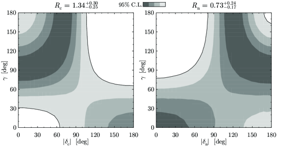
Figure 1: Constraints determined on the $|\delta_{\mathrm{(c,n)}}|,\gamma$ plane by the present CP averaged data on $B\rightarrow K\pi$.

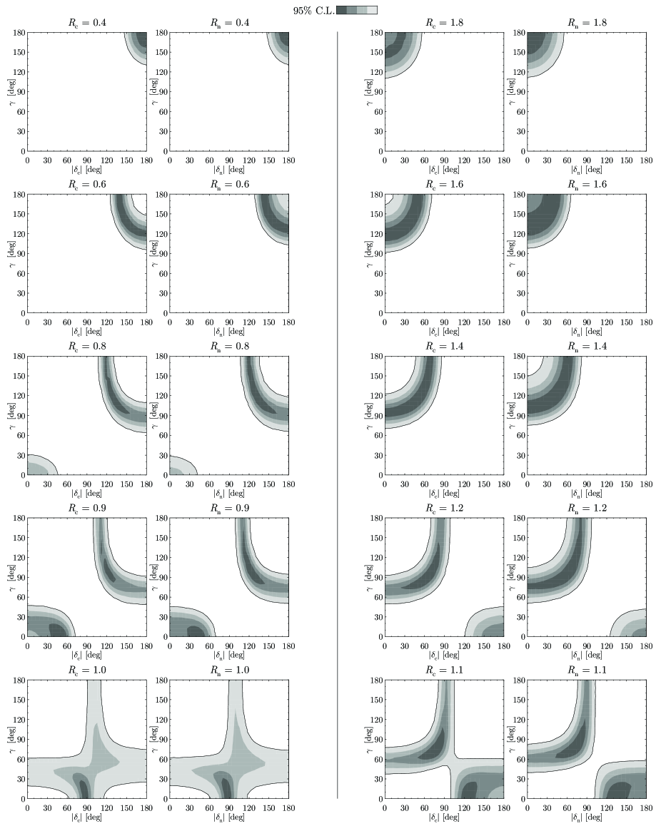
Figure 2: Constraints on the $|\delta_{\mathrm{(c,n)}}|,\gamma$ plane obtainable from precise measurements of $R_{\mathrm{n}}$ and $R_{\mathrm{c}}$.

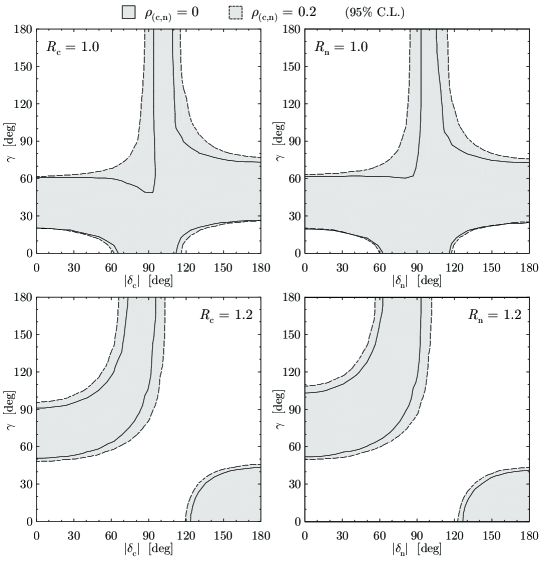
Figure 3: Examples of constraints on $\gamma$ and $\delta_{\mathrm{(c,n)}}$ obtainable from precise measurements of $R_{\mathrm{(c,n)}}=1.0$ and $R_{\mathrm{(c,n)}}=1.2$: the results in the absence of appreciable rescattering effects ($\rho_{\mathrm{(c,n)}}\simeq 0$) are compared with those obtained with the maximum value of $\rho_{\mathrm{(c,n)}}$ in the range assumed in the present analysis ($\rho_{\mathrm{(c,n)}}=0.2$). The contours, solid and dashed respectively, delimit regions allowed at the 95% C.L. in the two scenarios.

Figure 2 shows examples of how the determination of $\gamma$ and of the strong phases can evolve with improved measurements of the CP averaged branching ratios. For each value of $R_{\mathrm{c}}$ and $R_{\mathrm{n}}$, supposed to be measured with negligible experimental uncertainty, the graphs represent regions allowed at the $95\%$ C.L. in the $|\delta_{\mathrm{(c,n)}}|,\gamma$ plane, as determined exclusively by the indeterminacy assumed for the remaining parameters $qe^{i\omega}$, $r_{\mathrm{(c,n)}}$ and $\rho_{\mathrm{(c,n)}}e^{i\theta_{\mathrm{(c,n)}}}$ [Eq. (13)]. The following prospects can be outlined:

• A measured value of $R_{\mathrm{(c,n)}}$ smaller than $0.8$ determines a lower bound on both $\gamma$ and $|\delta_{\mathrm{(c,n)}}|$; the excluded ranges increase with decreasing value of $R_{\mathrm{(c,n)}}$. In an almost symmetrical way, if $R_{\mathrm{(c,n)}}$ assumes a value greater than $1.2$, it is possible to put a lower bound on $\gamma$ and an upper bound on $|\delta_{\mathrm{(c,n)}}|$. On the other hand, a precise measurement of $R_{\mathrm{(c,n)}}$ having a value included between 0.8 and 1.2 would not be sufficient by itself to delimit ranges of preferred values for $\gamma$ and $|\delta_{\mathrm{(c,n)}}|$.

• At the same time, measurements with values diverging from $R_{\mathrm{(c,n)}}\simeq 1$ are progressively in favour of the range $\gamma>90^{\circ}$ and therefore in contrast with the current SM determination of the UT [Eq. (14)].

• By fixing the strong phases (they can actually be calculated using different theoretical techniques [5, 18, 19]), it becomes possible to determine $\gamma$ even in the least favourable case of measurements of $R_{\mathrm{c}}$ and $R_{\mathrm{n}}$ with values near 1. To illustrate with an example, a sensitivity of $\Delta\gamma\sim 10^{\circ}$ can be reached, in that peculiar case, by constraining the strong phases $\delta_{\mathrm{c}}$ and $\delta_{\mathrm{n}}$ into the (hypothetical) range $[-30^{\circ},30^{\circ}]$.

• One interesting prospect is connected with the determination of the strong phases. It was pointed out [14] that the first measurements of $R_{\mathrm{c}}$ and $R_{\mathrm{n}}$ by CLEO favoured values of $\delta_{\mathrm{c}}$ and $\delta_{\mathrm{n}}$ which were markedly different from each other, in conflict with the approximate expectation $\delta_{\mathrm{c}}\simeq\delta_{\mathrm{n}}$. As can be seen in Fig. 1, no discrepancy between the values of $\delta_{\mathrm{c}}$ and $\delta_{\mathrm{n}}$ is implied by the present data. However, improved measurements will have the potential to establish such a contradiction: for example, measurements of $R_{\mathrm{c}}$ and $R_{\mathrm{n}}$ confirming the present central values, respectively greater than $1.2$ and smaller than $0.8$, at a sufficient level of precision (see Fig. 2) would point definitely to $|\delta_{\mathrm{c}}|<90^{\circ}$ and $|\delta_{\mathrm{n}}|>90^{\circ}$.

In the above examples, the unknown contribution of final state interactions to the $K^{0}\pi^{+}$ and $K^{0}\pi^{0}$ decay amplitudes has been parametrized by allowing $\rho_{\mathrm{c}}$ and $\rho_{\mathrm{n}}$ to be as large as $0.2$. A comparison between the most favourable scenario assuming $\rho_{\mathrm{c}}=\rho_{\mathrm{c}}=0$ and the one in which $\rho_{\mathrm{c}}$ and $\rho_{\mathrm{c}}$ are fixed to $0.2$ is shown in Fig. 3 for the two representative cases $R_{\mathrm{(c,n)}}=1.0$ and $R_{\mathrm{(c,n)}}=1.2$. As can be seen, the shape of the constraints remains almost the same in the two cases. Apparently, no crucial improvement in the determination of $\gamma$ at a fixed value of $\delta_{\mathrm{(c,n)}}$ could be obtained by further reducing the uncertainties related to the magnitude of the rescattering effects.

2.3 Constraints from CP asymmetries

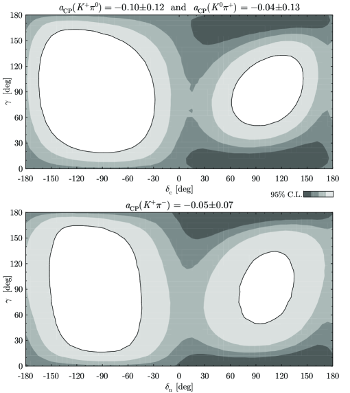
Figure 4: Constraints determined by the current CP asymmetry measurements: allowed regions in the $\delta_{\mathrm{(c,n)}},\gamma$ plane.

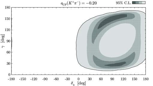
Figure 5: Example of constraint on the $\delta_{\mathrm{n}},\gamma$ plane as determined by a precise measurement of the direct CP asymmetry $a_{\mathrm{CP}}(K^{+}\pi^{-})$.

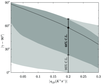
Figure 6: Ranges allowed for $|\gamma-90^{\circ}|$ at the 68% and 95% C.L. as a function of the measured value of $a_{\mathrm{CP}}(K^{+}\pi^{-})$.

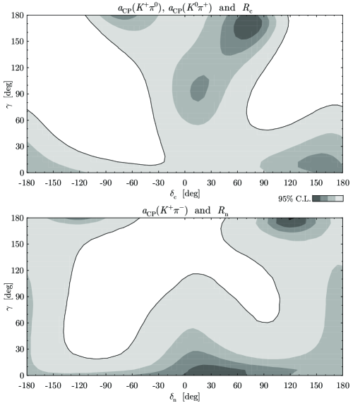
Figure 7: Preferred regions in the $\delta_{\mathrm{c}},\gamma$ and $\delta_{\mathrm{n}},\gamma$ planes, as determined by a global fit of the present $B\rightarrow K\pi$ rate and CP asymmetry measurements.

The constraints provided in the $\delta_{\mathrm{(c,n)}},\gamma$ plane by the first experimental results on the direct CP asymmetries are shown in Fig. 4. Here $a_{\mathrm{CP}}(K^{+}\pi^{0})$ and $a_{\mathrm{CP}}(K^{0}\pi^{+})$, both depending on the same subset of parameters (the one including $\rho_{\mathrm{c}}e^{i\theta_{\mathrm{c}}}$), are represented as a single constraint. The present data, still consistent with zero CP violation, determine an upper bound on $\gamma$ in the first quadrant and a lower bound in the second quadrant, almost symmetrically with respect to $\gamma=90^{\circ}$. The limit

$$|\gamma-90^{\circ}|>21^{\circ}\mathrm{\ \ at\ the\ }95\%\mathrm{\ C.L.}$$ (15)

can be derived from a fit of both constraints, with the strong phases $\delta_{\mathrm{c}}$ and $\delta_{\mathrm{n}}$ assumed as uniformly distributed over $[-180^{\circ},180^{\circ}]$.

Taking the decay $B^{0}\rightarrow K^{+}\pi^{-}$ as an example, Fig. 5 shows the constraint determined by a precise measurement of $a_{\mathrm{CP}}(K^{+}\pi^{-})=-0.20$ (examples with different central values are qualitatively very similar). As can be seen, a precise enough CP violation measurement would exclude a large portion of the $\delta_{\mathrm{n}},\gamma$ plane, being especially effective as a constraint on the strong phase; while the positive sign of $\delta_{\mathrm{n}}$ is selected in the case considered, the measurement of opposite sign, $a_{\mathrm{CP}}(K^{+}\pi^{-})=+0.20$, represented by the same plot after reflection with respect to the $\delta_{\mathrm{n}}=0$ axis, would point to $\delta_{\mathrm{n}}<0$.

As regards the determination of $\gamma$, the main implication of a measurement of CP violation with large enough central value would be the possibility of excluding two (almost symmetrical) regions around $\gamma=0$ and $\gamma=180^{\circ}$. Fig. 6 shows the intervals allowed for $|\gamma-90^{\circ}|$ at the 68% and 95% C.L., plotted as a function of the measured value of the CP asymmetry $a_{\mathrm{CP}}(K^{+}\pi^{-})$; only the absolute value of the asymmetry is considered here, in view of the fact that the constraint on $\gamma$ is not sensitive to the sign of the asymmetry when the strong phase is assumed as completely indeterminate.

Measurements of the CP asymmetry in $B^{+}\rightarrow K^{+}\pi^{0}$ determine almost the same constraints on $\gamma$ as those plotted in Fig. 6 for $B^{0}\rightarrow K^{+}\pi^{-}$, inasmuch as the only difference in the assumed ranges for the input parameters is the one between $r_{\mathrm{c}}$ and $r_{\mathrm{n}}$ [see Eqs. (5, 7, 13)]. The CP asymmetries in the decays $B^{+}\rightarrow K^{0}\pi^{+}$ and $B^{0}\rightarrow K^{0}\pi^{0}$, whose amplitudes depend on $\gamma$ only through the ‘corrective’ terms $\rho_{\mathrm{c}}e^{i(\theta_{\mathrm{c}}+\gamma)}$ and $\rho_{\mathrm{n}}e^{i(\theta_{\mathrm{n}}+\gamma)}$ respectively [Eqs. (4, 6)], have a minor role as constraints on $\gamma$, but may provide a confirmation of the smallness of the rescattering effects by placing upper limits on $\rho_{\mathrm{c}}$ and $\rho_{\mathrm{n}}$.

The results of a global fit of the present $B\rightarrow K\pi$ data, combining the CP averaged observables $R_{\mathrm{c}}$ and $R_{\mathrm{n}}$ and the direct CP asymmetries, are shown in Fig. 7.

2.4 Constraints on the $\bar{\rho},\bar{\eta}$ plane

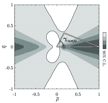
Figure 8: Constraints on the vertex $\bar{\rho},\bar{\eta}$ of the UT (95% probability regions) determined by the combination of the current experimental limits on the ratios of branching ratios and on the direct CP asymmetries. A typical UT configuration favoured by the current $|V_{ub}/V_{cb}|$, $\Delta m_{B_{d}}$ and $|\epsilon_{K}|$ constraints (see Ref. [24]) is shown for comparison.

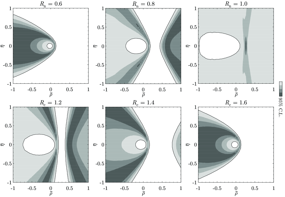
Figure 9: Constraints on the vertex $\bar{\rho},\bar{\eta}$ of the UT (95% probability regions), as determined by precise measurements of $R_{\mathrm{n}}$ and $R_{\mathrm{c}}$ with different central values.

Measurements of $R_{\mathrm{c}}$ and $R_{\mathrm{n}}$ and of the CP asymmetries can be included in a combined analysis of constraints on the vertex of the UT. Instead of using the experimental determination of $|V_{ub}/V_{cb}|$ to fix the value of the electroweak penguin parameter $qe^{i\omega}$ [Eq. (12)], one can rewrite Eq. (12) as

$$qe^{i\omega}=\frac{0.057}{\frac{\lambda}{1-\lambda^{2}/2}\sqrt{\bar{\rho}^{2}+\bar{\eta}^{2}}}$$ (16)

[besides, $\gamma=\arctan(\bar{\eta}/\bar{\rho})$] and fit the available experimental information using the variables $\bar{\rho}$ and $\bar{\eta}$. The constraints determined by the present measurements in the $\bar{\rho},\bar{\eta}$ plane are plotted in Fig. 8. The allowed region is compatible with the results of global fits of UT constraints [24], although smaller values of the CP violation parameter $\bar{\eta}$ are favoured by the $B\rightarrow K\pi$ data. Figure 9 illustrates the possible effect of precise measurements of $R_{\mathrm{c}}$ and $R_{\mathrm{n}}$.

3 Predictions for $R_{\mathrm{n}}$ and $R_{\mathrm{c}}$

As is illustrated by the examples shown in the previous Section, it is not possible to derive effective constraints on $\gamma$ in the first quadrant from precise measurements of $R_{\mathrm{c}}$ and $R_{\mathrm{n}}$, unless the strong phases $\delta_{\mathrm{c}}$ and $\delta_{\mathrm{n}}$ are known to assume certain fixed values. This limitation is the consequence of a destructive interference between tree and electroweak penguin amplitudes which occurs when $\gamma<90^{\circ}$ and is maximal for the specific value assumed by $qe^{i\omega}$ in the SM [Eq. (12)]. This accidental compensation results in a reduction of the sensitivity of $R_{\mathrm{c}}$ and $R_{\mathrm{n}}$ to the parameters $\gamma$ and $qe^{i\omega}$ and to the strong phases [see Eqs.(4, 5, 6, 7)]. This feature is illustrated in Fig. 10, which shows the dependence of $R_{\mathrm{c}}$ on the variables $\gamma$, $qe^{i\omega}$ and $\delta_{\mathrm{c}}$; for each scanned value, the remaining parameters are varied as indicated in Eq. (13); only the real values of $qe^{i\omega}$ are considered for simplicity. As can be seen, the spread of values of the ratio $R_{\mathrm{c}}$ is reduced considerably just next to the SM value of $qe^{i\omega}\simeq 0.65$ [Fig. 10(b)] and for $\gamma$ in the first quadrant [(Fig. 10(a)]. The wide variability outside these regions is mainly due to the assumed indeterminacy of the strong phase, as becomes evident when the value of $\delta_{\mathrm{c}}$ is constrained, for example, into the range $[-30^{\circ},30^{\circ}]$ [darker plots in the Figures 10(a) and 10(b)]. As a further example, the behaviour of the function $R_{\mathrm{c}}(\delta_{\mathrm{c}})$ plotted in Fig. 10(c-f) shows that the value of the SM prediction for $\gamma$ ($\sim 56^{\circ}$) implies a minimum sensitivity to the strong phase with respect to lower or, especially, higher values of $\gamma$.

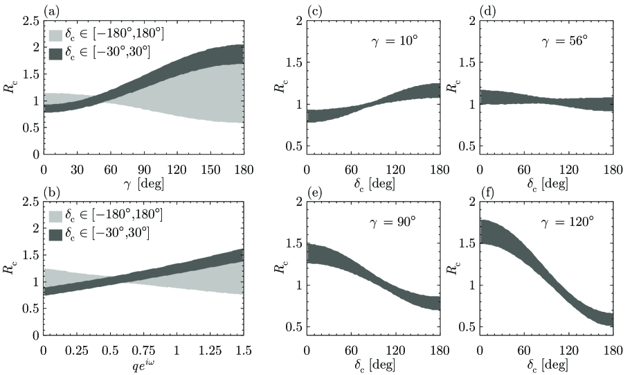
Figure 10: $R_{\mathrm{c}}$ as a function of $\gamma$ (a), of the electroweak penguin parameter $qe^{i\omega}$ (b) and of the strong phase $\delta_{\mathrm{c}}$ for different values of $\gamma$ (c, d, e, f). The intervals plotted for $R_{\mathrm{c}}$ are $\pm 1\sigma$ ranges.

The effective compensation between tree and electroweak penguin amplitudes when $\gamma$ is in the first quadrant reduces, on the one hand, the possibility of constraining the angle $\gamma$ with precise measurements; from a different point of view, it implies that for $\gamma<90^{\circ}$ the four $B\rightarrow K\pi$ decay amplitudes are actually dominated by their common QCD penguin components and that, consequently, values of the ratios $R_{\mathrm{c}}$ and $R_{\mathrm{n}}$ close to $1$ are strongly favoured in the SM. Probability distributions for $R_{\mathrm{c}}$ and $R_{\mathrm{n}}$ obtained by assuming the SM determination for $\gamma$ [Eq. (14)] are plotted in Fig. 11(a,b). They have been calculated by varying the input parameters according to Eq. (13). The 68% C.L. ranges derived from these distributions are

$$R_{\mathrm{c}}=1.03^{+0.07}_{-0.06}\qquad R_{\mathrm{n}}=1.02^{+0.07}_{-0.05},$$ (17)

while at the 95% C.L. both quantities are included between $0.9$ and $1.2$. As can be seen from the $R_{\mathrm{c}}\times R_{\mathrm{n}}$ plot shown in Fig. 11(c), there is no appreciable correlation between $R_{\mathrm{c}}$ and $R_{\mathrm{n}}$, the ratio $R_{\mathrm{c}}/R_{\mathrm{n}}$ being determined as

$$R_{\mathrm{c}}/R_{\mathrm{n}}=1.00^{+0.08}_{-0.07},$$

$$0.8<R_{\mathrm{c}}/R_{\mathrm{n}}<1.2\mathrm{\ \ at\ the\ }95\%\ \mathrm{C.L.}.$$ (18)

However, by expressing quantitatively the expectation that the strong phases $\delta_{\mathrm{c}}$ and $\delta_{\mathrm{n}}$ should have comparable values, the double ratio $R_{\mathrm{c}}/R_{\mathrm{n}}$ would become a very well determined quantity: for example, the hypothetical condition $|\delta_{\mathrm{c}}-\delta_{\mathrm{n}}|<60^{\circ}$ leads to a determination twice as precise:

$$(R_{\mathrm{c}}/R_{\mathrm{n}})_{{}_{|\delta_{\mathrm{c}}-\delta_{\mathrm{n}}|<60^{\circ}}}=1.00^{+0.05}_{-0.04},$$

$$0.9<(R_{\mathrm{c}}/R_{\mathrm{n}})_{{}_{|\delta_{\mathrm{c}}-\delta_{\mathrm{n}}|<60^{\circ}}}<1.1\mathrm{\ \ at\ the\ }95\%\ \mathrm{C.L.}.$$ (19)

The correlation between $R_{\mathrm{c}}$ and $R_{\mathrm{n}}$ introduced by this assumption is shown in Fig. 11(d).

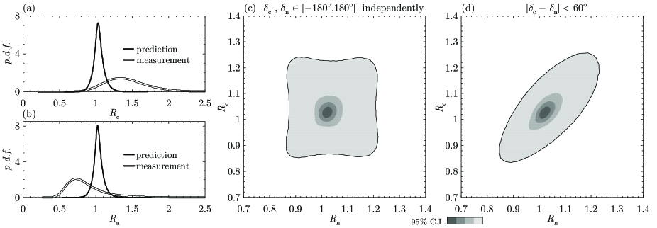
Figure 11: P.d.f.’s for $R_{\mathrm{c}}$ and $R_{\mathrm{n}}$ (a, b) and region allowed in the $R_{\mathrm{n}},R_{\mathrm{c}}$ plane for independent (c) and correlated (d) values of the strong phases.

The present experimental values [Eqs. (1, 2), with $R_{\mathrm{c}}/R_{\mathrm{n}}=1.6^{+0.6}_{-0.5}$] are compatible with the predictions obtained. Clearly, precise measurements are needed for a meaningful comparison with the expected values. It has to be pointed out that the SM expectation for $\gamma$ is not an essential ingredient of these predictions; a simple upper limit is sufficient to obtain quite precise values: with the only assumption that $\gamma<90^{\circ}$, the results

$$R_{\mathrm{c}}|_{\gamma<90^{\circ}}=1.02\pm 0.10,$$

$$R_{\mathrm{n}}|_{\gamma<90^{\circ}}=1.01^{+0.10}_{-0.09},$$ (20)

are obtained. The role of the uncertainty assumed in the present analysis to account for possible rescattering effects ($\rho_{\mathrm{c}}$ and $\rho_{\mathrm{n}}$ ranging from 0 up to 20%) is also marginal in these results, which remain essentially unchanged when $\rho_{\mathrm{c}}$ and $\rho_{\mathrm{n}}$ are set equal to zero assuming such effects to be absent ($R_{\mathrm{c}}|_{\rho_{\mathrm{c}}=0}=1.03\pm 0.06$, $R_{\mathrm{n}}|_{\rho_{\mathrm{n}}=0}=1.02^{+0.06}_{-0.05}$) or when they are fixed to the maximum value of the assumed range ($R_{\mathrm{c}}|_{\rho_{\mathrm{c}}=0.2}=1.03\pm 0.07$, $R_{\mathrm{n}}|_{\rho_{\mathrm{n}}=0.2}=1.02^{+0.07}_{-0.06}$). On the contrary, as can be seen from the $R(q)$ plot in Fig. 10(b), values of $R_{\mathrm{c}}$ and $R_{\mathrm{n}}$ inconsistent with the predictions in Eq. (17) may reflect large deviations from the assumed SM value of the EW parameter $qe^{i\omega}$ [Eq. (12)]. To illustrate with numerical examples, a measurement of $R_{\mathrm{c}}$ as large as $1.4$ could be accounted for by $qe^{i\omega}=1.2$ or, equivalently, by $qe^{i\omega}=0.65e^{i60^{\circ}}$, both leading to a determination of $R_{\mathrm{c}}$ included between $0.7$ and $1.4$ at the 95% C.L.. Therefore, precise measurements conflicting with the expectation $R_{\mathrm{c}}\simeq R_{\mathrm{n}}\simeq 1$ may be the sign of large SU(3)-breaking effects or new physics contributions to the electroweak penguin component of the decay amplitudes.

4 Conclusions

Experimental constraints on the weak ($\gamma$) and strong phases of the $B\rightarrow K\pi$ decay amplitudes have been studied in the model independent context of the flavour-SU(3) approach. The measured rates and CP asymmetries have been submitted to a global fit using the Bayesian method. Possible scenarios describing the impact of precise measurements have been reviewed in a wide range of hypothetical cases. Present situation and prospects are summarized in the following remarks:

• The precision of the CP averaged data has to be increased by about one order of magnitude in order to provide significant information on $\gamma$. On the other hand, the first experimental limits for the direct CP asymmetries exclude the range of values $69^{\circ}<\gamma<111^{\circ}$ at the 95% C.L..

• Even within the context of minimal theoretical assumptions which characterizes the SU(3) approach, the CP averaged observables related to $B\rightarrow K\pi$ decays can offer interesting prospects in the search for possible indications of new physics. Measurements of $R_{\mathrm{c}}$ and $R_{\mathrm{n}}$ not consistent with the range $0.8-1.2$ would in fact exclude the values of $\gamma$ in the first quadrant, at variance with the UT constraints derived from the $B-\bar{B}$ oscillation parameters $\Delta m_{s}$ and $\Delta m_{d}$. At the same time, precise measurements confirming the currently preferred values of $R_{\mathrm{c}}>1$ and $R_{\mathrm{n}}<1$ (or vice versa), would point to values of the strong phases $\delta_{\mathrm{c}}$ and $\delta_{\mathrm{n}}$ belonging to two different quadrants, in conflict with the theoretical expectation $\delta_{\mathrm{c}}\simeq\delta_{\mathrm{n}}$.

• On the other hand, measurements of $R_{\mathrm{c}}$ and $R_{\mathrm{n}}$ in the range $0.8-1.2$, though consistent with a value of $\gamma$ in the first quadrant, would not lead to an effective improvement of the UT determination.

• The strong phases $\delta_{\mathrm{c}}$ and $\delta_{\mathrm{n}}$ represent a crucial theoretical input to the analysis of the constraints on $\gamma$; with such additional information provided by direct calculations, a determination of $\gamma$ with $\Delta\gamma\simeq 10^{\circ}$ uncertainty becomes possible even in the least favourable case of measurements of $R_{\mathrm{c}}$ and $R_{\mathrm{n}}$ consistent with 1.

• On the contrary, the constraints on $\gamma$ obtainable from $R_{\mathrm{c}}$ and $R_{\mathrm{n}}$ are almost independent of the actual importance of rescattering effects, in so far as these are accounted for by values of $\rho_{\mathrm{c}}$ and $\rho_{\mathrm{n}}$ up to 0.2.

As an especially interesting result of the model independent phenomenological analysis that has been performed, well determined SM reference values are obtained for $R_{\mathrm{c}}$ and $R_{\mathrm{n}}$ when $\gamma$ is fixed to its SM expectation:

$$R_{\mathrm{c}}=1.03^{+0.07}_{-0.06}, R_{\mathrm{n}}=1.02^{+0.07}_{-0.05}.$$

These predictions rely mainly on the SU(3) estimates of the ratios of tree-to-QCD-penguin and of electroweak-penguin-to-tree amplitudes, being especially sensitive to the electroweak penguin component. They are on the other hand almost unaffected by the possible contribution of rescattering processes and only weakly dependent on the value assumed for $\gamma$ in the first quadrant. The expected improvement in the experimental precision will therefore offer the possibility of performing an interesting experimental test of SU(3) flavour-symmetry in the decays of $B$ mesons. At the same time, precise measurements definitely contradicting the expectation $R_{\mathrm{c}}\simeq R_{\mathrm{n}}\simeq 1$ should lead to the investigation of possible new physics effects in the electroweak penguin sector.

Acknowledgments

We are indebted to Robert Fleischer for useful discussions on the subject and most constructive comments on this work.

References

- [1] M. Gronau and D. London, Phys. Rev. Lett. 65, 3381 (1990).
- [2] A.J. Buras and R. Fleischer, Phys. Lett. B 360, 138 (1995).
- [3] R. Fleischer, Phys. Lett. B 459, 306 (1999).
- [4] R. Fleischer, Eur. Phys. J. C 16, 87 (2000).
- [5] A. Ali, G. Kramer, and C.-D. Lü, Phys. Rev. D 59, 014005 (1999).
- [6] M. Gronau, J.L. Rosner, and D. London, Phys. Rev. Lett. 73, 21 (1994).
- [7] R. Fleischer, Phys. Lett. B 365, 399 (1996).
- [8] R. Fleischer and T. Mannel, Phys. Rev. D 57, 2752 (1998).
- [9] A.J. Buras, R. Fleischer, and T. Mannel, Nucl. Phys. B533, 3 (1998).
- [10] R. Fleischer, Eur. Phys. J. C 6, 451 (1999).
- [11] M. Neubert and J.L. Rosner, Phys. Lett. B 441, 403 (1998); Phys. Rev. Lett. 81, 5076 (1998).
- [12] A.J. Buras and R. Fleisher, Eur. Phys. J. C 11, 93 (1999).
- [13] M. Neubert, J. High Energy Phys. 9902, 014 (1999).
- [14] A.J. Buras and R. Fleischer, Eur. Phys. J. C 16, 97 (2000).
- [15] D. Atwood and A. Soni, Phys. Lett. B 466, 326 (1999).
- [16] X.-G. He et al., Phys. Rev. D 64, 034002 (2001).
- [17] N.G. Deshpande, X.-G. He, W.-S. Hou, and S. Pakvasa, Phys. Rev. Lett. 82, 2240 (1999); X.-G. He, W.-S. Hou, and K.-C. Yang, ibid. 83, 1100 (1999); X.-G. He, C.-L. Hsueh, and J.-Q. Shi, ibid. 84, 18 (2000); W.-S. Hou and K.-C. Yang, Phys. Rev. D 61, 073014 (2000); M. Gronau and J.L. Rosner, ibid. 61, 073008 (2000); W.-S. Hou, J.G. Smith, and F. Würthwein (1999), hep-ex/9910014; H.-Y. Cheng and K.-C. Yang, Phys. Rev. D 62, 054029 (2000); B. Dutta and S. Oh, ibid. 63, 054016 (2001); W.-S. Hou and K.-C. Yang, Phys. Rev. Lett. 84, 4806 (2000); C. Isola and T.N. Pham, Phys. Rev. D 62, 094002 (2000); Y.-L. Wu and Y.-F. Zhou, ibid. 62, 036007 (2000); D. Du, D. Yang, and G. Zhu, Phys. Lett. B 488, 46 (2000); T. Muta, A. Sugamoto, M.-Z. Yang, and Y.-D. Yang, Phys. Rev. D 62, 094020 (2000); T.N. Pham, Nucl. Phys. B (Proc. Suppl.) 96, 467 (2001); W.-S. Hou (2000), hep-ph/0009197.
- [18] M. Beneke, G. Buchalla, M. Neubert, and C.T. Sachrajda, Nucl. Phys. B 606, 245 (2001).
- [19] Y.-Y. Keum, H.-N. Li, and A.I. Sanda, Phys. Lett. B 504, 6 (2001); Phys. Rev. D 63, 054008 (2001).
- [20] M. Ciuchini et al., hep-ph/0110022
- [21] D. Cronin-Hennessy et al. (CLEO Collaboration), Phys. Rev. Lett. 85, 515 (2000); S. Chen et al. (CLEO Collaboration), ibid. 85, 525 (2000).
- [22] K. Abe et al. (Belle Collaboration), Phys. Rev. Lett. 87, 101801 (2001); K. Abe et al. (Belle Collaboration), Phys. Rev. D 64, 071101 (2001).
- [23] B. Aubert et al. (BaBar Collaboration), Phys. Rev. Lett. 87, 151802 (2001); B. Aubert et al. (BaBar Collaboration), Phys. Rev. D 65, 051502 (2002).
- [24] M. Bargiotti et al., La Rivista del Nuovo Cimento, Vol. 23, N. 3 (2000) and P. Faccioli (2000), hep-ph/0011269; A. Ali and D. London, Eur. Phys. J. C 18, 665 (2001); M. Ciuchini et al., J. High Energy Phys. 07, 013 (2001); S. Mele, hep-ph/0103040; D. Atwood and A. Soni, Phys. Lett. B 508, 17 (2001); A. Höcker, H. Lacker, S. Laplace, and F. Le Diberder, Eur. Phys. J. C 21, 225 (2001).
- [25] Presentations and discussions at the Workshop on the CKM Unitarity Triangle, CERN, Geneva, February 13-16, 2002.
- [26] A.F. Falk, A.L. Kagan, Y. Nir, and A.A. Petrov, Phys. Rev. D 57, 4290 (1998).