TSL/ISV-2002-0262
April 2002

Abstract: The observed polarisation of $\Lambda$ hyperons from the inclusive $pA\rightarrow\Lambda X$ reaction at high energies has previously been well described within the Lund string model through polarised $s\bar{s}$ quark pair production in the string breaking hadronisation process. This model is here applied to the exclusive $\overline{p}p\rightarrow\overline{\Lambda}\Lambda$ reaction at low energies and compared to available data sets down to an incident beam momentum of 1.835 GeV/c. This required an extension of the diquark scattering model to involve three components: an isotropic part relevant close to threshold, a spectator part and a forward scattering part as in $pA\rightarrow\Lambda X$ at high energies. The observed angular distributions are then reproduced and, for momentum transfers above $|t^{\prime}|=0.2$ GeV², agreement with the measured polarisation is also obtained.

PACS numbers: 13.88.+e, 14.20.Jn

1 Introduction

In the mid 70’s it was discovered that $\Lambda$ hyperons produced by an unpolarised high–energy proton beam on an unpolarised target nucleus are polarised [1, 2]. This came as a big surprise since it was believed that spin effects would not survive at these high energies and perturbative QCD was indeed not able to describe the observations [3, 4].

Today, more than 20 years after these first observations, similar polarisation effects have been observed in a large energy range and for other hyperons of the baryon octet ($\Sigma^{-}$ [5], $\Sigma^{0}$ [6], $\Sigma^{+}$ [7], $\Xi^{-}$ [8] and $\Xi^{0}$ [9]). The trend of the data can be summarised as

$$P(\Lambda)\approx P(\Xi^{-})\approx P(\Xi^{0})\approx-P(\Sigma^{-})\approx-P(\Sigma^{0})\approx-P(\Sigma^{+}).$$

The understanding of the mechanism that produces polarised hyperons is, however, still far from complete and a wealth of different models have been proposed [10, 11, 12, 13, 14, 15]. The model discussed in this paper is an extension of a semiclassical model [11] that provides a good description of observed polarisation data for inclusively produced $\Lambda$ hyperons in $pA\rightarrow\Lambda X$ reactions. The model is based on the Lund string model [16], which successfully describes the hadronisation of quarks and gluons emerging from high energy interactions.

Most of the experimental data on hyperon polarisation come indeed from inclusive studies, but more recently also exclusive reactions have been studied [17, 18, 19], thus removing the uncertainty whether the observed $\Lambda$’s have been produced directly or stem from decays of heavier hyperons. In this paper we investigate whether the string-based model can be extended to describe exclusive hyperon production in the $\overline{p}p\rightarrow\overline{\Lambda}\Lambda$ reaction. Data obtained by the PS185 collaboration at LEAR, CERN, for this reaction [17] are of high precision and allow the validity of the model to be tested with high accuracy in the low energy domain (beam momenta below 2.0 GeV/c).

2 Basics of the string model

The original string model for polarisation is illustrated in Fig. 1a and described in this section.

Figure 1: (a) Inclusive $\Lambda$ production in the string model: A forward-scattered $(ud)_{0}$ diquark stretches a string field producing an $s\bar{s}$ pair, whose transverse momenta introduce an orbital angular momentum $\vec{L}$ pointing out of the scattering plane. To conserve the zero angular momentum in the string field, the $s$ and $\bar{s}$ spins are polarised in opposite direction.
(b) The string model adapted to $\overline{p}p\rightarrow\overline{\Lambda}\Lambda$: A $u$ and $\bar{u}$ annihilates giving $ud$ and $\bar{u}\bar{d}$ diquarks moving apart with opposite momenta ($q$) and an $s\bar{s}$ pair is produced (as in a), but with kinematical constraints for the exclusive production of $\Lambda\bar{\Lambda}$ in the c.m. system.

The incoming proton interacts with a target nucleon resulting in a forward-moving diquark system with transverse momentum $q_{T}$. A colour triplet string-field, with no transverse degrees of freedom, is stretched from this diquark (having an antitriplet colour charge) to a colour triplet charge in the collision region.

The potential energy in the field is reduced by breaking the string through the production of quark–antiquark pairs, i.e., colour triplet-antitriplet charges. Within the SU(6) constituent quark model, a $\Lambda$ consists of a $(ud)_{0}$ diquark ($I=S=0$) and an $s$ quark. Therefore, if the scattered diquark is a $(ud)_{0}$ quark pair and a strange–antistrange quark pair is produced in the string breaking, then a $\Lambda$ can be produced.

Transverse momentum is locally conserved and the $s$ and $\bar{s}$ quarks are therefore produced with equal but oppositely directed transverse momenta, $k_{T}$, relative to the string. For small scattering angles, the transverse momentum of the $\Lambda$ becomes $\vec{p}_{T}\approx\vec{q}_{T}+\vec{k}_{T}.$ The distributions in $k_{T}$ and $q_{T}$ are taken to be gaussian having widths $\sigma_{q_{T}}$ and $\sigma_{k_{T}}$, respectively. To account for $k_{T}$ and the strange quark mass $m_{s}\approx 0.2$ GeV/c², the $s$ and $\bar{s}$ are produced a distance $l=2\sqrt{m_{s}^{2}+k_{T}^{2}}/\kappa$ apart, such that energy stored in the string ($\kappa\approx 1\>GeV/fm$) is transformed to the transverse mass of the produced pair. This can be described as a virtual $s\bar{s}$ pair being produced in a single space–time point and then tunneling apart through the potential until they become on–shell. Treating this quantum mechanical tunneling process with the WKB method gives the gaussian $k_{T}$ spectrum used.

The separated $\vec{k}_{T}$–vectors produce an orbital angular momentum $L\>=\>lk_{T}$ of the $s\bar{s}$ pair. The key assumption of the model is that this orbital angular momentum is compensated by the polarisation of the spin of the $s$ and $\bar{s}$ in order to locally conserve the total angular momentum, which was zero in the string without transverse degrees of freedom. Since it is the $s$ quark that carries the spin of the $\Lambda$, the end result is the production of polarised $\Lambda$’s.

The model’s correlation between $k_{T}$ and the spin polarisation of the $s$ quark results in a $\Lambda$ polarisation which increase with its transverse momentum $p_{T}$. This may be viewed as a trigger bias effect, where a sample of $\Lambda$’s with a certain value of $\vec{p}_{T}$ will have an enhanced number of events where $\vec{k}_{T}$ points in the same direction and hence having a net polarisation.

In order for the compensation of orbital angular momenta by the quark spins to be consistent, it is necessary that the $k_{T}$ distribution is such that $L>1$ are suppressed. This is indeed the case, since $L>1$ corresponds to $k_{T}\hbox to0.0pt{\raise 2.0pt\hbox{$>$}\hss}{\lower 2.0pt\hbox{$\sim$}}0.3$ GeV/c with the values for $m_{s}$ and $\kappa$ quoted above. The dependence of the polarisation $P_{q}$ on $L$ is parameterised as $P_{q}\>=\>L/(\beta+L)$, with $\beta\sim 1$, such that the polarisation increases linearly for small $L$ and saturates at 100% for large $L$. The results are, however, rather insensitive to the particular function chosen to describe the $P_{q}$–$L$ correlation [11]. The model is numerically evaluated through a Monte Carlo simulation specifying momenta and polarisation event by event.

3 Model simulations for $\overline{\Lambda}$$\Lambda$ production

Measurements of the exclusive reaction $\overline{p}p\rightarrow\overline{\Lambda}\Lambda$ gives additional information as compared to inclusive $\Lambda$ production. The two-body kinematics imposes strong constraints that fixes the absolute value of the momenta of the two hyperons in the c.m. system. In order to apply the string–based model described above, it must be extended as illustrated in Fig. 1b. In the $p\bar{p}$ interaction a $u$ and $\bar{u}$ are annihilated leaving the $ud$ and $\bar{u}\bar{d}$ moving in opposite directions with equal momenta. Due to the fixed $\overline{\Lambda}$ ($\Lambda$) c.m. momentum, the diquark momentum $\vec{q}$ ($-\vec{q}$) is no longer independent of the momentum $\vec{k}_{T}$ ($-\vec{k}_{T}$) of the $\bar{s}$ ($s$) quark.

An important point of the above polarisation mechanism is that the $s$ and $\bar{s}$ have parallel spins and are therefore in a spin triplet state. Consequently, the model gives a natural explanation for the experimental fact [20] that the $\overline{\Lambda}\Lambda$ are dominantly in a spin triplet state.

Fig. 2 shows experimental results for the differential cross section for $\overline{p}p\rightarrow\overline{\Lambda}\Lambda$ obtained at $p_{\overline{p}}=6.0$ GeV/c. The data can be fitted with an empirical formula with two exponentials

$$d\sigma/dt^{\prime}=ae^{bt^{\prime}}+ce^{dt^{\prime}}$$ (1)

with slope parameters $b=10.1\pm 0.6$ GeV^-2 and $d=3.0\pm 0.3$ GeV^-2 [21]. Here, $t^{\prime}=-\frac{1}{2}t_{max}^{\prime}\left(1-\mbox{$\cos\Theta_{\overline{\Lambda}}^{*}$}\right)$ is the reduced four–momentum transfer squared, where mass effects are removed from the full four–momentum transfer

$$t=m^{2}_{p}+m^{2}_{\Lambda}-2s+\frac{1}{2}t_{max}^{\prime}\mbox{$\cos\Theta_{\overline{\Lambda}}^{*}$}$$

with $t_{max}^{\prime}=\sqrt{(s-4m^{2}_{p})\cdot(s-4m^{2}_{\Lambda})}$.

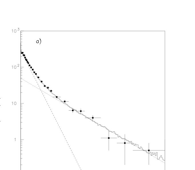
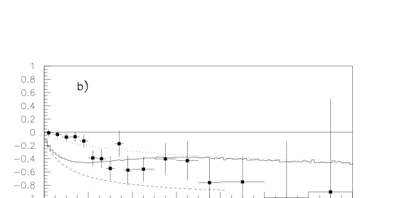
Figure 2: Experimental data [21] on (a) the differential cross section and (b) the polarisation in $\overline{p}p\rightarrow\overline{\Lambda}\Lambda$ taken at $p_{\overline{p}}=6.0$ GeV/c compared to string model simulations normalised to the total cross section of the data. The gaussian diquark $q_{T}$ distribution has $\sigma_{q_{T}}=0.45$ GeV (dotted line), $\sigma_{q_{T}}=0$ GeV (dashed line) and a 40%/60% mixture of these two (full line). In all cases $\sigma_{k_{T}}=0.3$ GeV is used.

The shape of the differential cross section obtained with the string model is also exponential in $t^{\prime}$, since $t^{\prime}\simeq p_{T}^{2}$ and, thereby, given by the gaussian $q_{T}$ and $k_{T}$ distributions. Using $\sigma_{q_{T}}=0.45$ GeV and $\sigma_{k_{T}}=0.3$ GeV one obtains the dotted line in Fig. 2a. These values are slightly lower than those ($\sigma_{q_{T}}=0.5$ GeV and $\sigma_{k_{T}}=0.35$ GeV) used in [11] to successfully describe $\Lambda$ polarisation in $pA\rightarrow\Lambda X$ at higher energies, but lead to practically the same results in that domain. The agreement of the model with the experimental $t^{\prime}$-distribution is good for $|t^{\prime}|\hbox to0.0pt{\raise 2.0pt\hbox{$>$}\hss}{\lower 2.0pt\hbox{$\sim$}}0.4$ GeV². For lower values of $|t^{\prime}|$ one obtains a good fit by setting $\sigma_{q_{T}}=0$ GeV (dashed line). These two parameter settings give the slopes $b=10.1$ GeV^-2 and $d=3.0$ GeV^-2 in good agreement with the experimental values. The Monte Carlo nature of the model makes it straight forward to add components with different parameter settings. A sum of simulations using a 60% contribution with $\sigma_{q_{T}}=0$ GeV and a 40% contribution with $\sigma_{q_{T}}=0.45$ GeV results in the solid line in Fig. 2a which reproduce the observed $t^{\prime}$-distribution very well.

We now turn to the polarisation which is shown as a function of $t^{\prime}$ in Fig. 2b. The original model with $\sigma_{q_{T}}=0.45$ GeV gives a decent description of the observed polarisation. With $\sigma_{q_{T}}=0$ GeV, the only source for transverse momentum is given by the $s$ ($\bar{s}$) quark momentum resulting in a very strong correlation between $p_{T}$ and the polarisation. This is reflected in the rapid increase of the polarisation for small values of $|t^{\prime}|$ shown by the dashed curve in Fig. 2b. The full curve represents the above 60%/40% mixture and gives a reasonable description of the polarisation for $|t^{\prime}|\hbox to0.0pt{\raise 2.0pt\hbox{$>$}\hss}{\lower 2.0pt\hbox{$\sim$}}0.2$ GeV², whereas at smaller $|t^{\prime}|$ the contribution of $\sigma_{q_{T}}=0$ overestimates the magnitude of the polarisation.

High precision data on the $\overline{p}p\rightarrow\overline{\Lambda}\Lambda$ reaction closer to threshold have been obtained by the PS185 collaboration at LEAR, CERN. A common feature in these data is that the angular distributions show, apart from the forward peaking, a more isotropic behaviour. This feature can not easily be explained by the model developed for higher energies. It can, however, be accommodated by adding an isotropic part to the diquark angular distribution. This would lead to zero polarisation since each $\Lambda$ scattering angle contains contributions of $\vec{k}_{T}$ and $-\vec{k}_{T}$ with equal probability.

Fig. 3 shows the simulated differential cross section with an added isotropic diquark component, and polarisation for $\overline{p}p\rightarrow\overline{\Lambda}\Lambda$ at 1.835 GeV/c. No contribution with $\sigma_{q_{T}}=0.45$ GeV is needed at this energy. The comparison with the data from PS185 shows that the polarisation is also here reasonably well reproduced for $|t^{\prime}|\hbox to0.0pt{\raise 2.0pt\hbox{$>$}\hss}{\lower 2.0pt\hbox{$\sim$}}0.2$ GeV². Note that the polarisation becomes zero at $t^{\prime}\approx-0.6$ GeV², corresponding to the c.m.s. scattering angle $\Theta_{\overline{\Lambda}}^{*}=90^{\circ}$ in agreement with experimental results for $p_{\mbox{$\overline{p}$}}>1.8$ GeV/c [22].

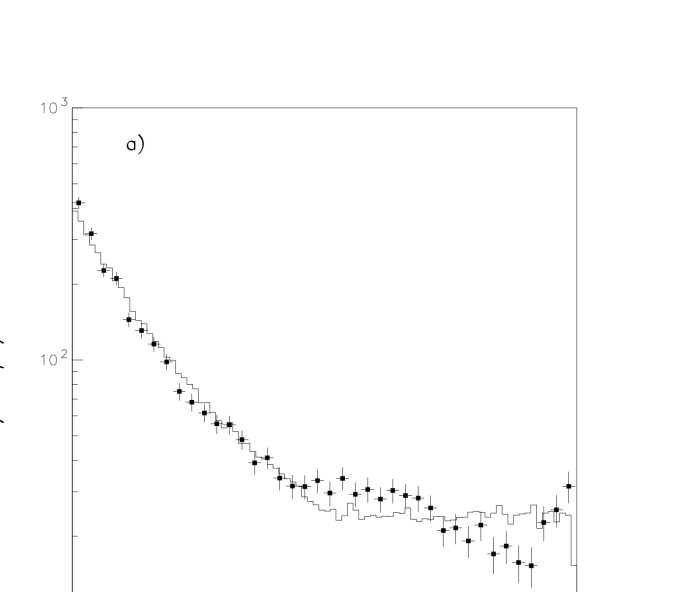
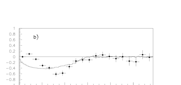
Figure 3: Comparison of the experimental data [23] at $p_{\overline{p}}=1.835$ GeV/c with a string model simulation having a 33% contribution of isotropic diquark scattering and the remainder with $\sigma_{q_{T}}=0$ GeV.

Fig. 4 shows the result of a simulation made at $p_{\overline{p}}=3.0$ GeV/c together with data from Refs. [24, 25]. For this intermediate energy, we again need a contribution with forward scattered diquarks ($\sigma_{q_{T}}=0.45$ GeV). The relative importance of the different contributions are discussed in next section.

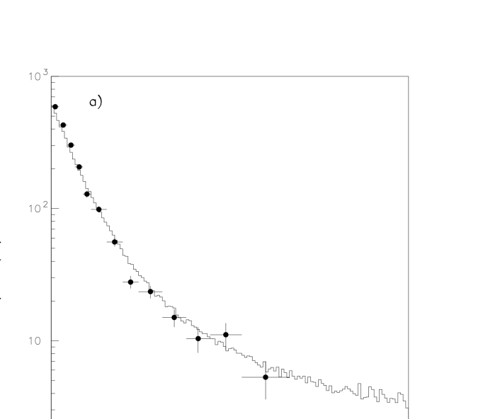
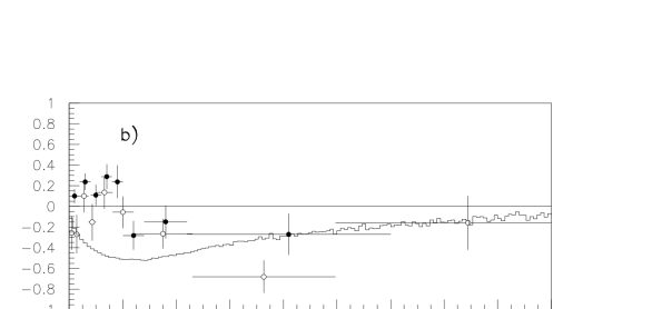
Figure 4: Comparison of experimental data (solid circles for $p_{\overline{p}}=3.0$ GeV/c [24] and open circles for $p_{\overline{p}}=3.6$ GeV/c [25]) for (a) the differential cross section and (b) the polarisation with string model simulations at $p_{\overline{p}}=3.0$ GeV/c (normalised to that data set). The diquark scattering has a 10% isotropic contribution, a 20% contribution with $\sigma_{q_{T}}=0.45$ GeV and a 70% contribution with $\sigma_{q_{T}}=0$ GeV ($\sigma_{k_{T}}=0.3$ GeV always).

Table 1 gives an overview of the parameters of Eq. 1 obtained from the model and fitted to the experimental data.

Table 1: Exponential slope parameters in Eq. (1) obtained by experiments in comparison with model simulation results.

$\overline{p}$ momentum	experiment		string model
(GeV/c)	$b$	$d$	$b$	$d$
6.0 [21]	$10.1\pm 0.6$	$3.0\pm 0.3$	10.1	3.0
3.6 [25]	$8.4\pm 0.4^{\dagger}$	$2.0\pm 0.2^{\dagger}$	9.0	1.8
3.0 [24]	$9.66\pm 0.47$	$1.58\pm 0.55$	8.9	1.8
1.8–2.0 [26]	8–9	–	6.5–7.5	–
†These values are obtained in our parameterisation
although [25] use a different parameterisation.

4 Discussion and conclusions

The Lund string model [16] for the hadronisation of high energy quarks and gluons gives a natural explanation for the polarisation of $\Lambda$’s produced in the inclusive reaction $pA\rightarrow\Lambda X$ at high energy [11]. A $(ud)_{0}$ diquark is here assumed to be scattered with a transverse momentum $q_{T}$ and stretching a colour string-field. In the breaking of this field an $s$ quark with transverse momentum $k_{T}$ is produced and a $\Lambda=(ud)_{0}s$ is formed with $\vec{p}_{T}=\vec{q}_{T}+\vec{k}_{T}$. The $s$ quark is polarised to compensate for an orbital angular momentum proportional to $k_{T}$, giving a polarisation of the $\Lambda$ which increases with its $p_{T}$. With the normal gaussian distributions in $k_{T}$ and $q_{T}$ used in the Lund model, the observed $\Lambda$ polarisation is reproduced [11].

An extension of this model has been developed here in order to test whether the same polarisation mechanism is able to reproduce also the polarisation observed in the two-body $\overline{p}p\rightarrow\overline{\Lambda}\Lambda$ reaction at low energy. The $s\bar{s}$ pair production in the string-field is supposed to be a local phenomenon in the string and is therefore expected to be energy independent. Therefore, we have not altered the gaussian $k_{T}$ distribution for the strange quarks, which is also the essential source of the polarisation. The diquark scattering mechanism, on the other hand, may very well be energy dependent. We have therefore extended the diquark scattering model to include three components: (1) forward scattered diquarks with $\sigma_{q_{T}}=0.45$ GeV, (2) diquarks as spectators without transverse momenta and (3) isotropic diquark scattering.

The first component, which was the only one included in the original model applied at high energies, becomes less important with decreasing $\overline{p}$ momentum; 40% at 6 GeV/c, 20% at 3 GeV/c and neglible below 2.0 GeV/c. On the other hand, the isotropic part is becoming more important closer to threshold. It is negligible at 6 GeV/c but increases to about 30% below 2 GeV/c. This reflects the fact that the $\overline{\Lambda}\Lambda$ pairs are produced in an S-wave at threshold. Diquarks as spectators contribute 60–70% at all energies. Since here, the diquarks have no transverse momenta ($\sigma_{q_{T}}=0$ GeV), it is only the ${k_{T}}$ of the strange quark that provides the transverse momentum and, therefore, $\sigma_{k_{T}}$ gives the slope of the $t^{\prime}$ distribution. This is reflected in the sharp forward rise in the angular distribution which is typical behaviour for peripheral processes. Using a the black–disc model, a slope of 8 GeV^-2 would correspond to an absorption radius of about 1 fm.

This string–based model cannot explain positive polarisation as observed in the region $|t^{\prime}|<0.2$ GeV². In the semiclassical picture we apply, this means that the diquarks pass each other at a distance of the order of the absorption radius, leading to an orbital angular momentum in the ($ud$)–($\overline{u}\overline{d}$) system. One may, therefore, imagine a scenario where both the orbital angular momentum of the $\overline{s}s$–pair and their spins compensate the angular momentum of the ($ud$)–($\overline{u}\overline{d}$) system. This would lead to positive polarisation in the very forward region (small $k_{T}$). For larger $k_{T}$ the $s\overline{s}$ angular momentum will overcompensate the ($ud$)–($\overline{u}\overline{d}$) angular momentum and we would again expect negative polarisation. To quantify this picture is, however, complicated since the orientation of the string, and thus $\vec{k}_{T}$ at the breakup, will vary with time.

The fact that the string model works quite well for larger momentum transfers, but not for smaller may give more fundamental insights. The border line $|t^{\prime}|\approx 0.2$ GeV² corresponds to a momentum transfer of a few hundred MeV. Above that, it is reasonable that a model formulated in a quark basis should be applicable since quark degrees of freedom can be resolved. For lower momentum transfers, however, even a constituent quark structure may be unresolved and it may be more appropriate to have a description in terms of hadrons. Such models formulated in a hadron basis have been considered in this context of $\overline{p}p\rightarrow\overline{\Lambda}\Lambda$, see, e.g., [27] and references therein. With suitable components of $K$ and $K^{*}$ exchange, including initial–state and final–state interactions, it is possible to obtain both the positive and negative polarisation. At this low energy scale it is not surprising that the full dynamical behaviour cannot be well described within the same simple quark–based model that works well at high energies.

In view of this, it is quite remarkable that the string–based model with only few parameters works so well for $\overline{p}p\rightarrow\overline{\Lambda}\Lambda$ at low energies. Both the observed angular distribution and, for not too small momentum transfers, also the polarisation in the $\overline{\Lambda}\Lambda$ system are well described. Moreover, the model gives a natural explanation for the fact that $\overline{\Lambda}\Lambda$ are produced in a spin triplet state. In total, this gives evidence for a universal origin of the $\Lambda$ polarisation phenomena observed at different energies.

References

- [1] A. Lesnik et al., Phys. Rev. Lett. 35 (1975) 770.
- [2] G. Bunce et al., Phys. Rev. Lett. 36 (1976) 1113.
- [3] G. L. Kane et al., Phys. Rev. Lett. 41 (1978) 1689.
- [4] R. Barni et al., Phys. Lett. B 296 (1992) 251.
- [5] L. Deck et al., Phys. Rev. D 28 (1983) 1.
-
[6]
E. C. Dukes et al., Phys. Lett. B 193 (1987) 135;
B. E. Bonner et al., Phys. Rev. Lett. 62 (1989) 1591. - [7] C. Wilkinson et al., Phys. Rev. Lett. 58 (1987) 855.
-
[8]
R. Rameika et al.,Phys. Rev. D 33 (1986) 3172;
J. Duryea et al., Phys. Rev. Lett. 67 (1991) 1193. -
[9]
P.T. Cox et al., Phys. Rev. Lett. 46 (1981) 877;
K. Heller et al., Phys. Rev. Lett. 51 (1983) 2025. - [10] K. Heller et al., Phys. Lett. B 68 (1977) 480.
- [11] B. Andersson et al., Phys. Lett. B 85 (1979) 417.
- [12] J. Szwed, Phys. Lett. B 105 (1981) 403.
- [13] T. A. DeGrand et al., Phys. Rev. D 23 (1981) 1227; Phys. Rev. D 24 (1981) 2419; Phys. Rev. D 31 (1985) 661 (E); Phys. Rev. D 32 (1985) 2445.
- [14] Liang Zou–tang and C. Boros, Phys. Rev. Lett. 79 (1997) 3608; ibid, Phys. Rev. D 61 (2000) 117503.
- [15] N. Nakajima, K. Suzuki, H. Toki and K.-I. Kubo, hep–ph/9906451.
- [16] B. Andersson et al., Phys. Rep., 97 (1983) 31 and B. Andersson, The Lund Model, Cambridge University Press, 1998.
- [17] P. D. Barnes et al., Phys. Lett. B 189 (1987) 249; Phys. Lett. B 199 (1987) 147; Phys. Lett. B 229 (1989) 432; Phys. Lett. B 246 (1990) 273; Nucl. Phys. A 526 (1991) 575; Phys. Lett. B 331 (1994) 203; Phys. Rev. C 54 (1996) 1877; Phys. Rev. C 54 (1996) 2831.
- [18] J. Félix et al., Phys. Rev. Lett. 76 (1996) 22.
- [19] F. Balestra et al., Phys. Rev. Lett. 83 (1999) 1534.
- [20] P. D. Barnes et al., Nucl. Phys. B 56A (1997) 46 and Nucl. Phys. A 655 (1999) 173c.
- [21] H. Becker et al., Nucl. Phys. B 141 (1978) 48.
- [22] For 1.835 GeV/c see Ref. [23], for 1.918 GeV/c see P. D. Barnes et al., Phys. Rev. C 54 (1996) 1877, for 1.949 and 1.992 GeV/c see Ref. [28]. Refs. [28, 29] also show the PS185 data from threshold up to the maximum energy. Fits to the polarisation data as function of the excess energy and are shown in Refs. [20, 29].
- [23] R.-A. Kraft, Untersuchung der Reaktion bei 1.835 GeV/c am Niederenergie–Antiprotonen–Speicherring LEAR, Ph. D. thesis, Universität Erlangen, 1994.
- [24] S. M. Jacobs et al., Phys. Rev. D 17 (1978) 1187.
- [25] H. W. Atherton et al., Nucl. Phys. B 69 (1974) 1.
- [26] M. Ziółkowski, Dynamik der Reaktion 170.5 MeV über der Produktionsschwelle, Ph. D. thesis, KFA Jülich, Jül-2703, 1992; R. Todenhagen, Strangenessproduktion in Antiproton–Proton–Stößen bei Einschußimpulsen um 1700 MeV/c, Ph. D. thesis, Universität Freiburg, 1995.
- [27] M.Alberg, Nucl. Phys. A 692 (2001) 47c.
- [28] R. Bröders, Spinobservable in der Strangenesserzeugung der Reaktion , Ph. D. thesis, Universität Bonn, Jül-3151, 1995.
- [29] S. Pomp, Hyperon Polarisation in the Reaction , Ph. D. thesis, Uppsala University, 1999.