Constraining Fourth Generation with $B\rightarrow X_{s}\gamma$

Using the theoretical and experimental results on $B\to X_{s}\gamma\,$, a four-generation SM is analyzed to constrain the combination of the $4\times 4$ Cabibbo-Kobayashi-Maskawa factor $V_{t^{\prime}s}^{\ast}V_{t^{\prime}b}$ as a function of the $t^{\prime}$–quark mass. It is observed that the results for the above–mentioned physical quantities are essentially different from the previous predictions for certain solutions of the CKM factor. Influences of the new model is used to predict CP violation in $B\to X_{s}\gamma\,$ decay at the order of $A_{CP}=5~{}\%$, stemming from the appearance of complex phases of $V_{t^{\prime}s}^{\ast}V_{t^{\prime}b}$ and of Wilson coefficients $C_{7}$, $C_{8}$, in the related process. The above mentioned physical quantities can serve as efficient tools in search of the fourth generation.

1 Introduction

Today, despite the success of the Standard Model (SM), from the theoretical point of view, it is incomplete. Number of generations of fermions can be mentioned as one of the open problems of SM, for which we do not have a clear argument to restrict the SM to three known generations. Mass of the extra generations, if ever exists, can be extracted from the measurements of neutrino experiments, which set a lower bound for extra generations ($m_{\nu_{4}}>45~{}GeV$) [1].

The idea of generalizing SM is not a new one. Probable effects of extra generations was studied in many works [2]–[17]. Generalizations of the SM can be used to introduce a new family, which was performed previously [18]. Using similar techniques, one can search fourth generation effects in B meson decays. The existing electroweak data on the $Z$–boson parameters, the $W$ boson and the top quark masses excluded the existence of the new generations with all fermions heavier than the $Z$ boson mass [17], nevertheless, the same data allows few extra generations, if neutral leptons have masses close to $50~{}GeV$.

$B\to X_{s}\gamma\,$ is one of the most promising areas in search of the fourth generation, via its indirect loop effects, which was performed previously [7, 8]. This decay is one of the most appropriate candidates to be searched in the extensions of SM, since we have solid experimental and theoretical background for the process under consideration.

In this work we study the contribution of the fourth generation in the rare $B\to X_{s}\gamma\,$ decay, to obtain constrains on the parameter space of the fourth generation. Our basic assumption is to fill the gap between theoretical and experimental results of $B\to X_{s}\gamma\,$, with the fourth generation. Of course, due to the mentioned assumption, decay width will change at the order of difference between theoretical and experimental results, however, predicted CP asymmetry is interesting when SM contribution is neglected. As it is well known, new physics effects can manifest themselves through the Wilson coefficients and their values can be different from the ones in the SM [19, 20], as well as through the new operators [21]. Note that the inclusive $B\rightarrow X_{s}\gamma$ decay have already been studied with the inclusion of the fourth generation [22, 23] to constrain $V_{t^{\prime}b}^{\ast}V_{t^{\prime}s}$. The restrictions of the parameter space of nonstandard models based on LO analysis are not as sensitive as in the case of NLO analysis. Therefore we preferred to work at NLO, for the decay under consideration.

On the experimental side, values related with the $B\to X_{s}\gamma\,$ are well known. First measurement of the $B\to X_{s}\gamma\,$ was performed by CLEO collaboration, leading to CLEO branching ratio  [24]

$$\mbox{$B\to X_{s}\gamma\,$}=(2.32\pm 0.57\pm 0.35)\times 10^{-4}\,.$$ (1)

In 1999, CLEO has presented an improved result [25]

$$\mbox{$B\to X_{s}\gamma\,$}=(3.15\pm 0.35\pm 0.32\pm 0.26)\times 10^{-4}\,.$$ (2)

The errors are statistical, systematic, and model dependent respectively. The rate measured by ALEPH [26] is consistent with the CLEO measurement. There exists also results of BELLE with a larger central value [27]:

$$\mbox{$B\to X_{s}\gamma\,$}=(3.37\pm 0.53\pm 0.42\pm 0.54)\times 10^{-4}\,.$$ (3)

Observing CP asymmetry in the decay $B\rightarrow X_{s}\gamma$ is interesting, presented by CLEO collaboration recently [28]

$$A_{CP}(B\rightarrow X_{s}\gamma)=(-0.079\pm 0.108\pm 0.022)\times(1.0\pm 0.030)\,,$$ (4)

for which prediction of the SM is $0.6~{}\%$ [29].

On the theoretical side, situation within and beyond the SM is well settled. A collective theoretical effort has led to the practical determination of $B\to X_{s}\gamma\,$ at the NLO, which was completed recently, as a joint effort of many different groups ([30],[31], [32], [33], [34],[35]). For a recent review, to complete the computation of NLO QCD corrections, we refer to ref. [36] and references therein. It is necessary to have precise calculations also in the extensions of the SM, which was performed for certain models [37]. With the appearance of more accurate data we will be able to provide stringent constraints on the free parameters of the models beyond SM. We can state that, the aim of the present paper is to obtain such constraints when the fourth generation is considered.

The paper is organized as follows. In section 2, we present the necessary theoretical expressions for the $B\to X_{s}\gamma\,$ decay in the SM with four generations, where we investigated the effect of introducing fourth generation at different scales upon branching ratio and CP asymmetry. Section 3 is devoted to the numerical analysis and our conclusion.

2 Theoretical results

We use the framework of an effective low-energy theory, obtained by integrating out heavy degrees of freedoms, which in our case W-boson and top quark and an additional $t^{\prime}$. Mass of the $t^{\prime}$ is at the order of $m_{W}$. In this approximation the effective Hamiltonian relevant for $b\rightarrow s\gamma$ decay reads [38, 39]

$${\cal H}_{eff} = \frac{4G_{F}}{\sqrt{2}}V_{ts}^{\ast}V_{tb}\sum_{i=1}^{8}{C}_{i}(\mu)\,{O}_{i}(\mu)~{},$$ (5)

where $G_{F}$ is the Fermi coupling constant $V$ is the Cabibbo-Kobayashi-Maskawa (CKM) quark mixing matrix, the the full set of the operators ${O}_{i}(\mu)$ and the corresponding expressions for the Wilson coefficients ${C}_{i}(\mu)$ in the SM can be found in ([30]–[34]).

In the model under consideration, the fourth generation is introduced in a similar way the three generations are introduced in the SM, no new operators appear and clearly the full operator set is exactly the same as in SM [39]. The fourth generation changes values of the Wilson coefficients $C_{7}(\mu_{W}),~{}C_{8}(\mu_{W})$, via virtual exchange of the fourth generation up quark $t^{\prime}$ at matching scale. With the definition $\lambda_{i}=V_{is}^{\ast}V_{ib},~{}i=\{u,~{}c,~{}t,~{}t^{\prime}\}$, the above mentioned Wilson coefficients, can be written in the following form

$$C_{7}^{eff}(\mu_{W}) = C_{7}^{SM}(\mu_{W})+\frac{\lambda_{t^{\prime}}}{\lambda_{t}}C_{7}^{New}(\mu_{W})~{},$$

$$C_{8}^{eff}(\mu_{W}) = C_{8}^{SM}(\mu_{W})+\frac{\lambda_{t^{\prime}}}{\lambda_{t}}C_{8}^{New}(\mu_{W})~{},$$ (6)

where the last terms in these expressions describe the contributions of the $t^{\prime}$ quark to the Wilson coefficients and $V_{t^{\prime}s}^{\ast}$ and $V_{t^{\prime}b}$ are the two elements of the $4\times 4$ Cabibbo–Kobayashi–Maskawa (CKM) matrix. The explicit forms of the $C_{i}^{New}$ can easily be obtained from the corresponding Wilson coefficient expressions in SM by simply substituting $m_{t}\rightarrow m_{t^{\prime}}$ (see [40, 41]). Neglecting the $s$ quark mass we can define the Wilson coefficients at the matching scale, where the LO functions are :

$$C_{7}^{SM} = \frac{x}{24}\,\frac{-8x^{3}+3x^{2}+12x-7+(18x^{2}-12x)\ln x}{(x-1)^{4}}\,$$

$$C_{8}^{SM} = \frac{x}{8}\,\frac{-x^{3}+6x^{2}-3x-2-6x\ln x}{(x-1)^{4}},\,$$ (7)

where ($x=m_{t}^{2}/m_{W}^{2}$).

In the calculations we used the NLO theoretical expressions, and different experimental values to constraint the $\lambda_{t^{\prime}}$ paramater. Since extended models are very sensitive to NLO corrections, we used the NLO expression for the branching ratio of the radiative decay $B\to X_{s}\gamma$, which has been presented in ref. [38]:

$$BR(B\to X_{s}\gamma) = BR(B\to X_{c}e\bar{\nu}_{e})\left|\frac{V_{ts}^{*}V_{tb}}{V_{cb}}\right|^{2}\frac{6\alpha_{e}}{\pi f(z)\kappa(z)}\frac{\bar{m}_{b}^{2}(\mu_{b})}{m_{b}^{2}}$$ (8)

$$\times\left(|D|^{2}+A\right)\left(1-\frac{\delta^{NP}_{SL}}{m_{b}^{2}}+\frac{\delta^{NP}_{\gamma}}{m_{b}^{2}}+\frac{\delta^{NP}_{c}}{m_{c}^{2}}\right)~{}.$$

Explicit forms of virtual, bremsstrahlung and non-perturbative parts of Eq. (8) can be found in [38, 36] and references therein. In the numerical analysis we obtained $B{\to}X_{s}\gamma$ branching ratio in the Standard Model $BR(\mbox{$B\to X_{s}\gamma\,$})=(3.48\pm 0.33)\times 10^{-4}$, which remains in agreement with the previous literature. But we considered only the central value in our analysis, with the expectation of absorbing errors into the different experimental values.

To obtain quantitative results we need the value of the fourth generation CKM matrix element $\lambda_{t^{\prime}}$. For this aim following [22], we will use the experimental results of the decays $BR(\mbox{$B\to X_{s}\gamma\,$})$ and determine the fourth generation CKM factor $\lambda_{t^{\prime}}$ When we consider the possible effects of the fourth generation, we demanded the theoretical value to be equal to the experimental values presented in the previous section. Which can be expressed as

$$BR(B\rightarrow X_{s}\gamma)_{4th} = \{2.66,~{}3.15,~{}3.37\}.$$ (9)

Theoretical results of the branching ratio for $m_{t^{\prime}}={75,...,500}~{}GeV$ values are obtained as as function of $\lambda_{t^{\prime}}$. Notice that in the expressions related with $BR(B\rightarrow X_{s}\gamma)_{4th}$, theoretical and experimental results are multiplied by a factor of $10^{4}$ . For instance when we chose $m_{t^{\prime}}=75$ GeV, and use the approach of Eq. (6):

$$BR(B\rightarrow X_{s}\gamma)_{4th} = 0.654502\,+\,6.69962\,\lambda_{t^{\prime}}+\,20.3501\,\lambda^{2}_{t^{{}^{\prime}}}+\,$$

$$0.396254\,|-0.305738-\,1.87828\,\lambda_{t^{\prime}}|^{2}+\,$$

$$23.9926\,|(\,-0.340878-\,0.0154077\,i)-(\,1.64283+\,0.05443\,i){\lambda_{t^{\prime}})|^{2}}\,.$$

When $\lambda_{t^{\prime}}$ is neglected branching ratio reduces to the re-scaled central value 3.48 of SM prediction. During the calculations we obtained similar expressions for different $m_{t^{\prime}}$ values. It suffices to present the case of a very heavy quark, for $m_{t^{\prime}}=~{}500~{}GeV$ :

$$BR(B\rightarrow X_{s}\gamma)_{4th} = 0.654502\,+\,20.9868\,\lambda_{t^{\prime}}+\,198.863\,{\lambda_{t^{\prime}}}^{2}+\,$$

$$0.396254\,|-0.305738-\,5.95621\,\lambda_{t^{\prime}}|^{2}+\,$$

$$23.9926\,|(\,-0.340878-\,0.0154077\,i)-(\,5.1664+\,0.11899\,i){\lambda_{t^{\prime}})|^{2}}\,.$$

In the numerical analysis, as a first step, ${\lambda_{t^{\prime}}}$ is assumed real and constraints are obtained as a function of mass of the extra generation top-quark $m_{t^{\prime}}$, and the values are presented in tab. (1) and can be obtained from fig.(1). Those values can also be extracted from the figures $(3,4,~{}and~{}5)$ (a) where the solution is the intersection point on the $BR_{\gamma}=1$ line . Notice that in the figures we normalized branching ratio to 1, using the experimental values 2.66, 3.15 and 3.37 respectively, hence $\lambda_{t^{\prime}}$ values can be obtained from the intersection points and this is true for all $figures$ except the ones related with $A_{CP}$ , presented in the following subsections.

$BR_{\gamma}$
                                                                                          $\lambda_{t^{\prime}}^{imaginary}$
                                       $\lambda_{t^{\prime}}^{real}$

Figure 1: $BR(B\rightarrow X_{s}\gamma)$ normalized to 1 with the experimental value $BR(\mbox{$B\to X_{s}\gamma\,$})=3.15$, in order to extract possible values of ${\lambda_{t^{\prime}}}$, for $m_{t^{\prime}}=75$ GeV. Constraints are obtained for Eq. (6), and can be inferred from the emerging circle.

$BR_{\gamma}$
                                                                                          $\lambda_{t^{\prime}}^{imaginary}$
                                       $\lambda_{t^{\prime}}^{real}$

Figure 2: As in Fig.1. $BR(B\rightarrow X_{s}\gamma)$ normalized to 1 with the experimental value $BR(\mbox{$B\to X_{s}\gamma\,$})=3.15$, but, constraints are obtained for Eq. (12)

$BR_{\gamma}$
                                           (a)                                                  (b)

Figure 3: $BR(B\rightarrow X_{s}\gamma)_{4th}$ normalized to 1, with the experimental value $BR(\mbox{$B\to X_{s}\gamma\,$})=2.66$. Red line stands for $m_{t^{\prime}}=75~{}GeV$, pink one denotes $m_{t^{\prime}}=500~{}GeV$, other masses are in this range respectively. Notice that in the figures ${\lambda_{t^{\prime}}}$ values are assumed real. Fig. (a). is related with Eq. (6) likewise, Fig. (b). is related with Eq. (12).

$BR_{\gamma}$
                                           (a)                                                  (b)

Figure 4: The same as Fig.3., for the experimental value $BR(\mbox{$B\to X_{s}\gamma\,$})=3.15$

$BR_{\gamma}$
                                           (a)                                                  (b)

Figure 5: The same as Fig.3., for the experimental value $BR(\mbox{$B\to X_{s}\gamma\,$})=3.37$

We also performed a very similar analysis for introducing the fourth generation effects at the $\mu_{b}$ scale to see the difference between the previous results. Following [22] it can be written as follows:

$$C_{7}^{eff}(\mu_{b}) = C_{7}^{SM}(\mu_{b})+\frac{\lambda_{t^{\prime}}}{\lambda_{t}}C_{7}^{New}(\mu_{b})~{},$$

$$C_{8}^{eff}(\mu_{b}) = C_{8}^{SM}(\mu_{b})+\frac{\lambda_{t^{\prime}}}{\lambda_{t}}C_{8}^{New}(\mu_{b})~{},$$ (12)

Using Eq.(9), and demanding theretical results to be equal to the experimental results again, we obtained following expression for $m_{t^{\prime}}=75$:

$$BR(B\rightarrow X_{s}\gamma)_{4th} = \,0.691542+\,23.9926\,\times\,$$ (13)

$$|(-0.340878-0.0154077\,i)-(8.13033+0.423786\,i)\lambda_{t^{\prime}}|^{2}\,$$

As another example for $m_{t^{\prime}}=500$ we obtained

$$BR(B\rightarrow X_{s}\gamma)_{4th} = \,0.691542+\,23.9926\,\times\,$$ (14)

$$|(-0.340878-0.0154077\,i)-(12.4566\,+0.484564\,i)\lambda_{t^{\prime}}|^{2}\,.$$

It is interesting to notice that, if we assume $\lambda_{t^{\prime}}$ can have imaginary parts, experimental values can also be satisfied. This case is presented with a graphical solution in figure (2) for $m_{t}=75$ and the decomposition $\lambda_{t^{\prime}}=\lambda_{t}^{real}\,+\,i\,\lambda_{t}^{imaginary}$. When $\lambda_{t^{\prime}}$ is assumed real constraints can be extracted from figures (3,4, and  5) (b) on the normalized line. Real and imaginary parts or this approach is presented in tables (2) and (3) respectively.

$$\begin{array}[]{|c|c|c|c|c|c|c|c|}\hline\cr\vrule\lx@intercol\hfil BR(\mbox{$B\to X_{s}\gamma\,$})=2.66\times 10^{-4}\hfil\lx@intercol\vrule\lx@intercol\\ \hline\cr{m_{t^{\prime}}~{}(GeV)}&75&100&150&200&300&400&500\\ \hline\cr\hline\cr\lambda_{t^{\prime}}^{(I)}\times 10^{-1}&-3.63&-2.85&-2.04&-1.72&-1.42&-1.29&-1.22\\ \hline\cr\lambda_{t^{\prime}}^{(II)}\times 10^{-3}&-1.01&-0.75&-0.54&-0.45&-0.37&-0.34&0.32\par\\ \hline\cr\vrule\lx@intercol\hfil BR(\mbox{$B\to X_{s}\gamma\,$})=3.15\times 10^{-4}\hfil\lx@intercol\vrule\lx@intercol\\ \hline\cr{m_{t^{\prime}}~{}(GeV)}&75&100&150&200&300&400&500\\ \hline\cr\hline\cr\lambda_{t^{\prime}}^{(III)}\times 10^{-1}&-3.90&-2.90&-2.08&-1.74&-1.45&-1.31&-1.25\\ \hline\cr\lambda_{t^{\prime}}^{(IV)}\times 10^{-3}&-3.4&-2.5&-1.8&-1.5&-1.2&-1.1&-1.1\\ \hline\cr\vrule\lx@intercol\hfil BR(\mbox{$B\to X_{s}\gamma\,$})=3.37\times 10^{-4}\hfil\lx@intercol\vrule\lx@intercol\\ \hline\cr{m_{t^{\prime}}~{}(GeV)}&75&100&150&200&300&400&500\\ \hline\cr\hline\cr\lambda_{t^{\prime}}^{(V)}\times 10^{-1}&-3.67&-2.73&-1.96&-1.63&-1.35&-1.23&-1.12\\ \hline\cr\lambda_{t^{\prime}}^{(VI)}\times 10^{-3}&-2.6&-1.9&-1.4&-1.1&-1.0&-0.9&-0.8\\ \hline\cr\hline\cr\end{array}$$

Table 1: The numerical (real parts only) values of $\lambda_{t^{\prime}}$ for different values of the $m_{t^{\prime}}$ –quark mass and experimental values . The superscripts $(I),...,(VI)$ correspond to first and last solutions of Eq. (9) with the approximation of Eq. (12).

$$\begin{array}[]{|c|c|c|c|c|c|c|c|}\hline\cr\vrule\lx@intercol\hfil BR(\mbox{$B\to X_{s}\gamma\,$})=2.66\times 10^{-4}\hfil\lx@intercol\vrule\lx@intercol\\ \hline\cr{m_{t^{\prime}}~{}(GeV)}&75&100&150&200&300&400&500\\ \hline\cr\hline\cr\lambda_{t^{\prime}}^{(I)}\times 10^{-2}&-8.81&-7.03&-6.27&-5.85&-5.41&-5.17&-5.03\\ \hline\cr\lambda_{t^{\prime}}^{(II)}\times 10^{-3}&-7.76&-6.18&-5.51&-5.13&-4.74&-4.53&-4.41\\ \hline\cr\vrule\lx@intercol\hfil BR(\mbox{$B\to X_{s}\gamma\,$})=3.15\times 10^{-4}\hfil\lx@intercol\vrule\lx@intercol\\ \hline\cr{m_{t^{\prime}}~{}(GeV)}&75&100&150&200&300&400&500\\ \hline\cr\hline\cr\lambda_{t^{\prime}}^{(III)}\times 10^{-2}&-9.29&-7.41&-6.61&-5.70&-5.45&-5.30&-5.09\\ \hline\cr\lambda_{t^{\prime}}^{(IV)}\times 10^{-3}&-3.03&-2.41&-2.14&-1.99&-1.84&-1.76&-1.71\\ \hline\cr\vrule\lx@intercol\hfil BR(\mbox{$B\to X_{s}\gamma\,$})=3.37\times 10^{-4}\hfil\lx@intercol\vrule\lx@intercol\\ \hline\cr{m_{t^{\prime}}~{}(GeV)}&75&100&150&200&300&400&500\\ \hline\cr\hline\cr\lambda_{t^{\prime}}^{(V)}\times 10^{-2}&-9.49&-7.56&-6.74&-6.29&-5.81&-5.56&-5.41\\ \hline\cr\lambda_{t^{\prime}}^{(VI)}\times 10^{-3}&-1.07&-0.84&-0.75&-0.69&-0.64&-0.61&-0.59\\ \hline\cr\hline\cr\end{array}$$

Table 2: The numerical values of $\lambda_{t^{\prime}}$ for different values of the $m_{t^{\prime}}$ –quark mass and experimental values . The superscripts $(I),...,(VI)$ correspond to first and last solutions of Eq. (9) with the approximation of Eq. (6). Notice that in this table real values of $\lambda_{t^{\prime}}$ is presented only. In table 3 imaginary parts can be found.

$$\begin{array}[]{|c|c|c|c|c|c|c|c|}\hline\cr\vrule\lx@intercol\hfil BR(\mbox{$B\to X_{s}\gamma\,$})=2.66\times 10^{-4}\hfil\lx@intercol\vrule\lx@intercol\\ \hline\cr{m_{t^{\prime}}~{}(GeV)}&75&100&150&200&300&400&500\\ \hline\cr\hline\cr\lambda_{t^{\prime}}^{(I)}\times 10^{-2}&0.28&0.17&0.13&0.11&0.09&0.08&0.07\\ \hline\cr\lambda_{t^{\prime}}^{(II)}\times 10^{-3}&-0.17&-0.14&-0.13&-0.12&-0.11&-0.11&-0.10\\ \hline\cr\vrule\lx@intercol\hfil BR(\mbox{$B\to X_{s}\gamma\,$})=3.15\times 10^{-4}\hfil\lx@intercol\vrule\lx@intercol\\ \hline\cr{m_{t^{\prime}}~{}(GeV)}&75&100&150&200&300&400&500\\ \hline\cr\hline\cr\lambda_{t^{\prime}}^{(III)}\times 10^{-2}&-0.31&-0.19&-0.15&-0.11&-0.09&-0.08&-0.07\\ \hline\cr\lambda_{t^{\prime}}^{(IV)}\times 10^{-3}&-2.10&-1.68&-1.50&-1.41&-1.30&-1.25&-1.21\\ \hline\cr\vrule\lx@intercol\hfil BR(\mbox{$B\to X_{s}\gamma\,$})=3.37\times 10^{-4}\hfil\lx@intercol\vrule\lx@intercol\\ \hline\cr{m_{t^{\prime}}~{}(GeV)}&75&100&150&200&300&400&500\\ \hline\cr\hline\cr\lambda_{t^{\prime}}^{(V)}\times 10^{-2}&-0.32&-0.19&-0.15&-0.13&-0.11&-0.09&-0.09\\ \hline\cr\lambda_{t^{\prime}}^{(VI)}\times 10^{-3}&-2.1&-1.6&-1.5&-1.4&-1.3&-1.24&-1.21\\ \hline\cr\hline\cr\end{array}$$

Table 3: Imaginary parts of $\lambda_{t^{\prime}}$ values, presented in table 2.

In order to check the consistency of the results of present work one can demand $\lambda_{t^{\prime}}$ values to satisfy the unitarity condition. If we impose the unitarity condition of the CKM matrix we then have

$$\lambda_{u}+\lambda_{c}+\lambda_{t}+\lambda_{t^{\prime}}=0~{}.$$ (15)

With the values of the CKM matrix elements in the SM [43], the sum of the first three terms in Eq. (15) is about $7.6\times 10^{-2}$, where the error in sum of first three terms is about $\pm 0.6\times 10^{-2}$. By substituting the values of $\lambda_{t^{\prime}}$ from tables 1 and 2, we observe that the sum of the four terms on the left–hand side of Eq. (15) may get very close to zero or diverge from the prediction of SM . When $\lambda_{t^{\prime}}$ is very close to the sum of the first three terms, but with opposite sign, this is a very desirable result. Using table 2 for $m_{t^{\prime}}=100$ GeV and the experimental branching ratio $3.37\times 10^{-}4$, our prediction reads $\lambda^{(V)}_{t^{\prime}}=-7.56\times 10^{-2}$. On the other hand the same prediction contains an imaginary part $-0.19\,i\times 10^{-2}$, which may be absorbed within the error range. In other words, results presented in table (2) satisfy unitarity constrain to a good extend. Nevertheless, it is a matter of taste to accept or reject $\lambda_{t^{\prime}}$ values, according to unitarity condition. Because, it is possible that , existence of extra generations can affect present constraints on $V_{CKM}$ to a certain extend, and hence, constraints may get relaxed [44], which is beyond the scope of this work. From this respect it is hard to claim that all results presented here can satisfy unitarity. Nevertheless, in order to give the full picture, we did not exclude regions that violates unitarity.

2.1 Differences in the definitions of $\lambda_{t^{\prime}}$

In order to explain the difference, on the results of the two different approaches given in Eq. (6) and Eq. (12) or tables (1) and (2), we can perform the analysis in LO, to extract the value of the fourth generation CKM matrix element $\lambda_{t^{\prime}}$. Following [20], one can use the experimental results of the decays $BR(\mbox{$B\to X_{s}\gamma\,$})$ and $BR(B\to X_{c}e\bar{v}_{e})$, as in [42]. In order to reduce the uncertainties arising from $b$ quark mass, consider the following ratio

$$R=\frac{Br(B\to X_{s}\gamma)}{Br(B\to X_{c}e\bar{v}_{e})}\,.$$ (16)

In leading logarithmic approximation, for low energy scale approximation ratio can be written as

$$R=\alpha_{m}|C^{\rm eff}_{7}(\mu_{b})|^{2}$$ (17)

where $\alpha_{m}=\frac{|V^{*}_{ts}V_{tb}|^{2}}{|V_{cb}|^{2}}\frac{6\alpha}{\pi f(\hat{m}_{c})\kappa(\hat{m}_{c})}$ , the phase factor $f(\hat{m}_{c})$ and ${\cal O}(\alpha_{s})$, QCD correction factor $\kappa(\hat{m}_{c})$ of $b\to cl\bar{\nu}$ are given in ref.[45]. Using the LO definition of $C^{eff}_{7}(\mu_{b})$ one can write [46],

$$C^{eff}_{7}(\mu_{b})=\eta^{16/23}C^{eff}_{7}(\mu_{W})+\frac{8}{3}(\eta^{14/23}-\eta^{16/23})C^{eff}_{8}(\mu_{W})+C^{eff}_{2}(\mu_{W})\sum^{8}_{i=1}h_{i}\eta^{a_{i}}$$ (18)

for the present purpose, which can be written as

$$C^{eff}_{7}(\mu_{b})=\eta_{1}\,C^{eff}_{7}(\mu_{W})+\eta_{2}\,C^{eff}_{8}(\mu_{W})+\eta_{3}\,C^{eff}_{2}(\mu_{W})$$ (19)

When the effect of 4-generation it is defined as Eq. (12)

$$C_{7,8}^{eff}(\mu_{b}) = C_{7,8}^{SM}(\mu_{b})+\frac{\lambda_{t^{\prime}}}{\lambda_{t}}C_{7,8}^{New}(\mu_{b})~{},$$

solution of Eq. (17) for $\lambda_{t^{\prime}}$ can be written as follows

$$\lambda_{t^{\prime}}^{\pm}=\left[\pm\sqrt{\frac{R}{\alpha_{m}}}-C_{7}^{\rm SM}(\mu_{b})\right]\frac{\lambda_{t}}{C_{7}^{\rm New}(\mu_{b})}\,.$$ (21)

whereas in the case of the following approach ( Eq. (12))

$$C_{7,8}^{eff}(\mu_{W}) = C_{7,8}^{SM}(\mu_{W})+\frac{\lambda_{t^{\prime}}}{\lambda_{t}}C_{7,8}^{New}(\mu_{W})~{},$$

Eq. (21) is modified into the following form

$$\lambda_{t^{\prime}}^{\pm}=\left[\pm\sqrt{\frac{R}{\alpha_{m}}}-C_{7}^{\rm SM}(\mu_{b})\right]\frac{\lambda_{t}}{\left[\eta_{1}\,C_{7}^{\rm New}(\mu_{b})+\eta_{2}\,C_{8}^{\rm New}(\mu_{b})\right]}\,.$$ (23)

This analysis can also be performed for NLO expressions. By comparing Eq. (21) and Eq. (23) the difference in tables (1) and and (2) can be inferred. It should be stressed that, for Eq.(17), possibility of a complex solution for $\lambda_{t^{\prime}}$ should not be excluded.

2.2 Direct CP violation in $B\to X_{s}\gamma\,$

Observation of CP violation in $B\to X_{s}\gamma\,$ is attractive, because it could lead to an evidence related with the new physics. Theoretical predictions for $B\to X_{s}\gamma\,$ can be written as

$$A_{CP}({B\rightarrow X_{s}\,\gamma})=\frac{\Gamma(\bar{B}\rightarrow X_{s}\gamma)-\Gamma(B\rightarrow X_{\bar{s}}\gamma)}{\Gamma(\bar{B}\rightarrow X_{s}\gamma)+\Gamma(B\rightarrow X_{\bar{s}}\gamma)}\,.$$

Numerically, prediction of the SM is [29]

$$A_{CP}({B\rightarrow X_{s}\gamma})\approx 0.6\%,\qquad$$ (24)

when the best-fit values for the CKM parameters [47] are used. From the experimental side, we have the CLEO measurement of the CP asymmetry in the $b\rightarrow s\gamma$ decays [28],

$$A_{CP}(B\rightarrow X_{s}\gamma)=(-0.079\pm 0.108\pm 0.022)\times(1.0\pm 0.030)\,,$$ (25)

We used the CP asymmetry formulae to look for 4 generation effects [29],

$$A_{CP}({B\rightarrow X_{s}\,\gamma})\simeq\frac{10^{-2}}{|C_{7}|^{2}}(1.17\times{\rm Im}\left[C_{2}C_{7}^{*}\right]-9.51\times{\rm Im}\left[C_{8}C_{7}^{*}\right]$$ (26)

$$+0.12\times{\rm Im}\left[C_{2}C_{8}^{*}\right]-9.40\times{\rm Im}\left[\epsilon_{s}C_{2}\left(C_{7}^{*}-0.013\;C_{8}^{*}\right)\right]);$$

$$\epsilon_{s}=\frac{V_{us}^{*}V_{ub}}{V_{ts}^{*}V_{tb}}\simeq-\lambda^{2}(\rho-i\eta).\quad\quad$$

As it is stated in the same reference, the large coefficient of the second term in (26) is very attractive.

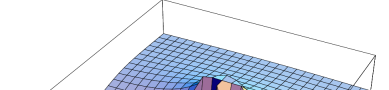
$A_{CP}\times 10^{2}$
                                                                                                ${\lambda_{t^{\prime}}}^{imaginary}$
                                     ${\lambda_{t^{\prime}}}^{real}$

Figure 6: $A_{CP}(B\rightarrow X_{s}\gamma)$ for $m_{t^{\prime}}=~{}75$.

We observed that, enhanced chromomagnetic dipole contribution, $C_{8}$, induces a large direct CP violation in the decay $B\rightarrow X_{s}\gamma$. This is due to complex phases of $\lambda_{t^{\prime}}$, which in result affects $C_{7},~{}C_{8}$. Such an enhancement of the chromomagnetic contribution may lead to a natural explanation of the phenomenology of semileptonic $B$ decays and charm production in $B$ decays [48, 29].

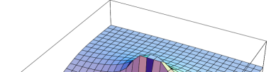
$A_{CP}\times 10^{2}$
                                                                                                ${\lambda_{t^{\prime}}}^{imaginary}$
                                     ${\lambda_{t^{\prime}}}^{real}$

Figure 7: $A_{CP}(B\rightarrow X_{s}\gamma)$ for $m_{t^{\prime}}=~{}50$.

Notice that in $A_{CP}$ figures, when the real values of $\lambda_{t^{\prime}}$ is around $-6\times 10^{-2}$, even for very small imaginary parts, peak values of $A_{CP}$ can be observed. Evolution of $A_{CP}({B\rightarrow X_{s}\,\gamma})$ is presented in figures $\{7,8,9,10\}$. CP asymmetry is not sensitive to very heavy $m_{t^{\prime}}$ quark masses.

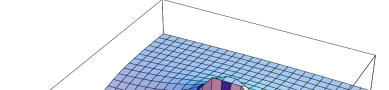
$A_{CP}\times 10^{2}$
                                                                                                ${\lambda_{t^{\prime}}}^{imaginary}$
                                     ${\lambda_{t^{\prime}}}^{real}$

Figure 8: $A_{CP}(B\rightarrow X_{s}\gamma)$ for $m_{t^{\prime}}=~{}100$.

$A_{CP}\times 10^{2}$
                                                                                                ${\lambda_{t^{\prime}}}^{imaginary}$
                                     ${\lambda_{t^{\prime}}}^{real}$

Figure 9: $A_{CP}(B\rightarrow X_{s}\gamma)$ for $m_{t^{\prime}}=~{}300$.

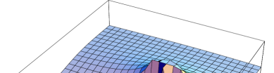
$A_{CP}\times 10^{2}$
                                                                                                ${\lambda_{t^{\prime}}}^{imaginary}$
                                     ${\lambda_{t^{\prime}}}^{real}$

Figure 10: $A_{CP}(B\rightarrow X_{s}\gamma)$ for $m_{t^{\prime}}=~{}500$.

3 Conclusion

To summarize, the $B\to X_{s}\gamma\,$ decay has a clean experimental and theoretical base, very sensitive to the various extensions of the Standard Model, can be used to constrain the fourth generation model. In the present work, this decay is studied in the SM with the four generation model. The solutions of the fourth generation CKM factor $\lambda_{t^{\prime}}$ have been obtained. It is observed that different choices of the factor $\lambda_{t^{\prime}}$, could be very informative, especially due to new CP violation effects, in searching new physics.

CP asymmetry in the $B\to X_{s}\gamma\,$ decay can be enhanced up to $5~{}\%$, which is ten times larger compared to the SM prediction. Hence it could be mentioned among the probes of new physics, especially in the case of fourth generation.

References

[1] P. Abreu et al., (DELPHI Collaboration),
Phys. Lett.B274 (1992) 23.
[2] X. G. He and S. Paksava,
Nucl. Phys.B278 (1986) 905.
[3] A. Anselm et al.,
Phys. Lett.B156 (1985) 103.
[4] U. Turke et al.,
Nucl. Phys.B258 (1985) 103.
[5] I. Bigi,
Z. Phys.C27 (1985) 303.
[6] G. Eilam, J. L. Hewett and T. G. Rizzo,
Phys. Rev.D34 (1986) 2773.
[7] W. S. Hou and R. G. Stuart,
Phys. Rev.D43 (1991) 3669.
[8] N. G. Deshpande, J. Trampetic,
Phys. Rev.D40 (1989) 3773.
[9] G. Eilam, B. Haeri and A. Soni,
Phys. Rev.D41 (1990) 875; Phys. Rev. Lett.62 (1989) 719.
[10] N. Evans,
Phys. Lett.B340 (1994) 81.
[11] P. Bamert and C. P. Burgess,
Z. Phys.C66 (1995) 495.
[12] T. Inami et al.,
Mod. Phys. Lett.A10 (1995) 1471.
[13] A. Masiero et al.,
Phys. Lett.B355 (1995) 329.
[14] V. Novikov, L. B. Okun, A. N. Rozanov et al.,
Mod. Phys. Lett.A10 (1995) 1915; Erratum. ibidA11 (1996) 687; Rep. Prog. Phys.62 (1999) 1275.
[15] Y. Dincer, Phys.Lett. B505 (2001) 89-93.
[16] J. Erler, P. Langacker,
Eur. J. Phys.C3 (1998) 90.
[17] M. Maltoni et al.,
prep. hep–ph/9911535 (1999).
[18] J. F. Gunion, D. McKay and H. Pois,
Phys. Rev.D51 (1995) 201;
[19] T. Goto, Y. Okada, Y. Shimizu and M. Tanaka,
Phys. Rev.D58 (1998) 094006.
[20] C. S. Huang and S. H. Zhu,
Phys. Rev.D61 (2000) 015011.
[21] T. M. Aliev and E. İltan
J. Phys. G.25 (1999) 989.
[22] C. S. Huang, W. J. Huo and Y. L. Wu,
prep. hep–ph/9911203 (1999).
[23] T. M. Aliev et al.
Nucl. Phys. B.585 (2000) 275.
[24]
M. S. Alam et al. [CLEO Collaboration], Phys. Rev. Lett. 74, 2885
(1995).
[25]
S. Ahmed et al. [CLEO Collaboration], hep-ex/9908022.
[26]
R. Barate et al. [ALEPH Collaboration], Phys. Lett. B429, 169 (1998).
[27]
P. Chang [BELLE Collaboration],
Nucl. Phys. A 684, 704 (2001);
B. A. Shwartz [Belle Collaboration],
Nucl. Phys. Proc. Suppl. 93, 332 (2001);
B. G. Cheon [BELLE Collaboration],
Nucl. Phys. Proc. Suppl. 93, 83 (2001);
K. Kinoshita [BELLE Collaboration], Nucl. Instrum. Meth. A
462, 77 (2001)
[hep-ex/0101033];
see also http://bsunsrv1.kek.jp/ .
[28]
T. E. Coan et al. [CLEOF Collaboration], hep-ex/0010075.
[29] T. Hurth, [hep-ph/0106060]
[30]
A. Ali and C. Greub, Z. Phys. C 49, 431 (1991); Phys. Lett. B 361, 146 (1995) [hep-ph/9506374].
[31]
N. Pott, Phys. Rev. D54, 938 (1996) [hep-ph/9512252].
[32]
C. Greub, T. Hurth and D. Wyler, Phys. Lett. B 380, 385 (1996)
[hep-ph/9602281]; Phys. Rev. D 54, 3350 (1996)
[hep-ph/9603404].
[33]
K. Adel and Y. Yao,Phys. Rev. D 49, 4945 (1994)
[hep-ph/9308349].
[34]
K. Chetyrkin, M. Misiak and M. Munz, Phys. Lett. B400, 206
(1997) [hep-ph/9612313].
[35]
C. Greub and T. Hurth, Phys. Rev. D 56, 2934 (1997)
[hep-ph/9703349].
[36] A. J. Buras, A. Carnecki, M. Misiak and J.
Urban hep-ph/0203135
[37]
C. Bobeth, M. Misiak and J. Urban, Nucl. Phys. B 567, 153 (2000) [hep-ph/9904413].
[38] K. Chetyrkin, M. Misiak and M. Münz, Phys. Lett. B400 (1997) 206.
[39] J. Hewett, “Top ten models constrained by ”,
published in proceedings “Spin structure in
high energy processes”, p. 463, Stanford, 1993.
[40] A. J. Buras and M. Münz,
Phys. Rev.D52 (1995) 186.
[41] B. Grinstein, M. J. Savage and M. B. Wise,
Nucl. Phys.B319 (1989) 271.
[42] C. S. Lim, T. Morozumi and A. I. Sanda,
Phys. Lett.B218 (1989) 343.
[43] C. Caso et al.,
Eur. J. Phys.C3 (1998) 1.
[44]
C. Hamzaoui, M.E. Pospelov, Phys.Lett. B357 (1995) 616-623.
[45] A. J. Buras, [hep-ph/9806471]
[46] A. J. Buras M.Misiak M. Münz. S. Pokorski, Nucl. Phys.B424 (1994) 374-398.
[47]
F. Caravaglios, F. Parodi, P. Roudeau and A. Stocchi,
hep-ph/0002171.
[48]
A. L. Kagan and M. Neubert, Phys. Rev. D 58, 094012 (1998) [hep-ph/9803368].