BNL-NT-02/5

Classical Chromo–Dynamics of
Relativistic Heavy Ion Collisions

Abstract

Relativistic heavy ion collisions produce thousands of particles, and it is sometimes difficult to believe that these processes allow for a theoretical description directly in terms of the underlying theory – QCD. However once the parton densities are sufficiently large, an essential simplification occurs – the dynamics becomes semi–classical. As a result, a simple ab initio approach to the nucleus–nucleus collision dynamics may be justified. In these lectures, we describe the application of these ideas to the description of multi–particle production in relativistic heavy ion collisions. We also discuss the rôle of semi–classical fields in the QCD vacuum in hadron interactions at low and high energies.

guessConjecture

1 What is Chromo–Dynamics?

Strong interaction is, indeed, the strongest force of Nature. It is responsible for over $80\%$ of the baryon masses, and thus for most of the mass of everything on Earth and in the Universe. Strong interactions bind nucleons in nuclei, which, being then bound into molecules by much weaker electro-magnetic forces, give rise to the variety of the physical World. Quantum Chromo–Dynamics is the theory of strong interactions, and its practical importance is thus undeniable. But QCD is more than a useful tool – it is a consistent and very rich field theory, which continues to serve as a stimulus for, and testing ground of, many exciting ideas and new methods in theoretical physics.

These lectures will deal with QCD of strong color fields, which can be explored in relativistic heavy ion collisions. (See the lectures by E. Iancu, A. Leonidov, L. McLerran [Iancu, Leonidov, McLerran (2002)], A.H. Mueller [Mueller (2001)], and R. Venugopalan in this volume for complementary presentation of the subject and more details.)

1.1 QCD: the Lagrangean

So what is QCD? From the early days of the accelerator experiments it has become clear that the number of hadronic resonances is very large, suggesting that all hadrons may be classified in terms of a smaller number of (more) fundamental constituents. A convenient classification was offered by the quark model, but QCD was not born until the hypothetical existence of quarks was not supplemented by the principle of local gauge invariance, previously established as the basis of electromagnetism. The resulting Lagrangian has the form

$${\cal{L}}=-{1\over 4}G_{\mu\nu}^{a}G_{\mu\nu}^{a}+\sum_{f}\bar{q}_{f}^{a}(i\gamma_{\mu}D_{\mu}-m_{f})q_{f}^{a};$$ (1)

the sum is over different colors $a$ and quark flavors $f$; the covariant derivative is $D_{\mu}=\partial_{\mu}-igA_{\mu}^{a}t^{a}$, where $t^{a}$ is the generator of the color group $SU(3)$, $A_{\mu}^{a}$ is the gauge (gluon) field and $g$ is the coupling constant. The gluon field strength tensor is given by

$$G_{\mu\nu}^{a}=\partial_{\mu}A_{\nu}^{a}-\partial_{\nu}A_{\mu}^{a}+gf^{abc}A_{\mu}^{b}A_{\nu}^{c},$$ (2)

where $f^{abc}$ is the structure constant of $SU(3)$: $[t^{a},t^{b}]=if^{abc}t^{c}$.

1.2 Asymptotic freedom

Due to the quantum effects of vacuum polarization, the charge in field theory can vary with the distance. In electrodynamics, summation of the electron–positron loops in the photon propagator leads to the following expression for the effective charge, valid at $r\gg r_{0}$:

$$\alpha_{em}(r)\simeq{3\pi\over 2\ln(r/r_{0})}.$$ (3)

This formula clearly exhibits the “zero charge” problem [Landau and Pomeranchuk (1955)] of QED: in the local limit $r_{0}\to 0$ the effective charge vanishes at any finite distance away from the bare charge due to the screening. Fortunately, because of the smallness of the physical coupling, this apparent inconsistency of the theory manifests itself only at very short distances $\sim exp\{-3\pi/[2\alpha_{em}]\},\ \alpha_{em}\simeq 1/137$. Such short distances are (and probably will always remain) beyond the reach of experiments, and one can safely use QED as a truly effective theory.

As it has been established long time ago [Gross and Wilczek; Politzer (1973)], QCD is drastically different from electrodynamics in possessing the remarkable property of “asymptotic freedom” – due to the fact that gluons carry color, the behavior of the effective charge $\alpha_{s}=g^{2}/4\pi$ changes from the familiar from QED screening to anti–screening:

$$\alpha_{s}(r)\simeq{3\pi\over(11N_{c}/2-N_{f})\ln(r_{0}/r)};$$ (4)

as long as the number of flavors does not exceed $16$ ($N_{c}=3$), the anti–screening originating from gluon loops overcomes the screening due to quark–antiquark pairs, and the theory, unlike electrodynamics, is weakly coupled at short distances: $\alpha_{s}(r)\to 0$ when $r\to 0$.

1.3 Chiral symmetry

In the limit of massless quarks, QCD Lagrangian (1) possesses an additional symmetry $U_{L}(N_{f})\times U_{R}(N_{f})$ with respect to the independent transformation of left– and right–handed quark fields $q_{L,R}={1\over 2}(1\pm\gamma_{5})q$:

$$q_{L}\to V_{L}q_{L};\ \ q_{R}\to V_{R}q_{R};\ \ V_{L},V_{R}\in U(N_{f});$$ (5)

this means that left– and right–handed quarks are not correlated. Even a brief look into the Particle Data tables, or simply in the mirror, can convince anyone that there is no symmetry between left and right in the physical World. One thus has to assume that the symmetry (5) is spontaneously broken in the vacuum. The flavor composition of the existing eight Goldstone bosons (3 pions, 4 kaons, and the $\eta$) suggests that the $U_{A}(1)$ part of $U_{L}(3)\times U_{R}(3)=SU_{L}(3)\times SU_{R}(3)\times U_{V}(1)\times U_{A}(1)$ does not exist. This constitutes the famous “$U_{A}(1)$ problem”.

1.4 The origin of mass

There is yet another problem with the chiral limit in QCD. Indeed, as the quark masses are put to zero, the Lagrangian (1) does not contain a single dimensionful scale – the only parameters are pure numbers $N_{c}$ and $N_{f}$. The theory is thus apparently invariant with respect to scale transformations, and the corresponding scale current is conserved: $\partial_{\mu}s_{\mu}=0$. However, the absence of a mass scale would imply that all physical states in the theory should be massless!

1.5 Quantum anomalies and classical solutions

Both apparent problems – the missing $U_{A}(1)$ symmetry and the origin of hadron masses – are related to quantum anomalies. Once the coupling to gluons is included, both flavor singlet axial current and the scale current cease to be conserved; their divergences become proportional to the $\alpha_{s}G_{\mu\nu}^{a}\tilde{G}_{\mu\nu}^{a}$ and $\alpha_{s}G_{\mu\nu}^{a}G_{\mu\nu}^{a}$ gluon operators, correspondingly. This fact by itself would not have dramatic consequences if the gluonic vacuum were “empty”, with $G_{\mu\nu}^{a}=0$. However, it appears that due to non–trivial topology of the $SU(3)$ gauge group, QCD equations of motion allow classical solutions even in the absence of external color source, i.e. in the vacuum. The well–known example of a classical solution is the instanton, corresponding to the mapping of a three–dimensional sphere $S^{3}$ into the $SU(2)$ subgroup of $SU(3)$; its existence was shown to solve the $U_{A}(1)$ problem.

1.6 Confinement

The list of the problems facing us in the study of QCD would not be complete without the most important problem of all – why are the colored quarks and gluons excluded from the physical spectrum of the theory? Since confinement does not appear in perturbative treatment of the theory, the solution of this problem, again, must lie in the properties of the QCD vacuum.

1.7 Understanding the Vacuum

As was repeatedly stated above, the most important problem facing us in the study of all aspects of QCD is understanding the structure of the vacuum, which, in a manner of saying, does not at all behave as an empty space, but as a physical entity with a complicated structure. As such, the vacuum can be excited, altered and modified in physical processes [Lee and Wick (1974)].

2 Strong interactions at short and large distances

In this lecture we will investigate the influence of QCD vacuum on hadron interactions at short and large distances. To make the problem treatable, we will limit ourselves to heavy quarkonia. In this lecture I will describe two recent results – one on the scattering of heavy quarkonia at very low energies, another on high–energy scattering. The common idea behind these two examples is to explore the influence of the QCD vacuum on hadron interactions. The presentation will be schematic, and I refer the interested reader to the original papers [Fujii and Kharzeev (1999)] and [Kharzeev and Levin (2000)] for details.

2.1 The long–range forces of QCD

2.1.1 Perturbation theory

Let us begin with a somewhat academic problem – the scattering of two heavy quarkonium states at very low energies. The Wilson operator product expansion allows one to write down the scattering amplitude (in the Born approximation) of two small color dipoles in the following form[Bhanot and Peskin (1977)]:

$$V(R) = -i\int dt\langle 0|\mbox{T}\left(\sum_{i}c_{i}O_{i}(0)\right)\left(\sum_{j}c_{j}O_{j}(x)\right)|0\rangle,$$ (6)

where $x=(t,R)$, $O_{i}(x)$ is the set of local gauge-invariant operators expressible in terms of gluon fields, and $c_{i}$ are the coefficients which reflect the structure of the color dipole. At small (compared to the binding energy of the dipole) energies, the leading operator in (6) is the square of the chromo-electric field $(1/2)g^{2}{\bf E}^{2}$ [Voloshin (1978), Bhanot and Peskin (1977)]. Keeping only this leading operator, we can rewrite (6) in a simple form

$$V(R) = -i\Big{(}\bar{d}_{2}\frac{a_{0}^{2}}{\epsilon_{0}}\Big{)}^{2}\int dt\langle 0|\mbox{T}\ \frac{1}{2}g^{2}{\bf E}^{2}(0)\ \frac{1}{2}g^{2}{\bf E}^{2}(t,R)|0\rangle,$$ (7)

where $\bar{d}_{2}$ is the corresponding Wilson coefficient defined by

$$\bar{d}_{2}\frac{a_{0}^{2}}{\epsilon_{0}}=\frac{1}{3N}\langle\phi|r^{i}\frac{1}{H_{a}+\epsilon}r^{i}|\phi\rangle,$$ (8)

where we have explicitly factored out the dependence on the quarkonium Bohr radius $a_{0}$ and the Rydberg energy $\epsilon_{0}$; $N$ is the number of colors, and $|\phi\rangle$ is the quarkonium wave function, which is Coulomb in the heavy quark limit. In physical terms, the structure of (7) is transparent: it describes elastic scattering of two dipoles which act on each other by chromo-electric dipole fields; color neutrality permits only the square of dipole interaction. It is convenient to express $g^{2}{\bf E}^{2}$ in terms of the gluon field strength tensor [Novikov and Shifman (1981)]:

$$g^{2}{\bf E}^{2}=-\frac{1}{4}g^{2}G_{\alpha\beta}G^{\alpha\beta}+g^{2}(-G_{0\alpha}G_{0}^{\alpha}+\frac{1}{4}g_{00}G_{\alpha\beta}G^{\alpha\beta})=$$

$$=\frac{8\pi^{2}}{b}\theta_{\mu}^{\mu}+g^{2}\theta_{00}^{(G)}$$ (9)

where

$$\theta_{\mu}^{\mu}\equiv\frac{\beta(g)}{2g}G^{\alpha\beta a}G_{\alpha\beta}^{a}=-\frac{bg^{2}}{32\pi^{2}}G^{\alpha\beta a}G_{\alpha\beta}^{a}\ .$$ (10)

Note that as a consequence of scale anomaly, $\theta_{\mu}^{\mu}$ is the trace of the energy-momentum tensor of QCD in the chiral limit of vanishing light quark masses.

Let us now introduce the spectral representation for the correlator of the trace of energy-momentum tensor:

$$\langle 0|\mbox{T}\theta_{\mu}^{\mu}(0)\theta_{\mu}^{\mu}(x)|0\rangle=\int d\sigma^{2}\rho_{\theta}(\sigma^{2})\Delta_{F}(x;\sigma^{2}),$$ (11)

where $\rho_{\theta}(\sigma^{2})$ is the spectral density and $\Delta_{F}(x;\sigma^{2})$ is the Feynman propagator of a scalar field. Using the representation (11) in (7), we get

$$V_{\theta}(R) = -\Big{(}\bar{d}_{2}\frac{a_{0}^{2}}{\epsilon_{0}}\Big{)}^{2}\Big{(}\frac{4\pi^{2}}{b}\Big{)}^{2}\int d\sigma^{2}\rho_{\theta}(\sigma^{2})\frac{1}{4\pi R}e^{-\sigma R}.$$ (12)

The potential (12) is simply a superposition of Yukawa potentials corresponding to the exchange of scalar quanta of mass $\sigma$.

Our analysis so far has been completely general; the dynamics enters through the spectral density. In perturbation theory, for $SU(N)$, one has

$$\rho^{\rm pt}_{\theta}(q^{2}) = \left(\frac{bg^{2}}{32\pi^{2}}\right)^{2}\frac{N^{2}-1}{4\pi^{2}}q^{4}.$$ (13)

Substituting (13) into (12) and performing the integration over invariant mass $\sigma^{2}$, we get, for $N=3$

$$V_{\theta}(R) = -g^{4}\Big{(}\bar{d}_{2}\frac{a_{0}^{2}}{\epsilon_{0}}\Big{)}^{2}\frac{15}{8\pi^{3}}\frac{1}{R^{7}}.$$ (14)

The $\propto R^{-7}$ dependence of the potential (14) is a classical result known from atomic physics [Casimir and Polder (1948)]; as is apparent in our derivation (note the time integration in (12)), the extra $R^{-1}$ as compared to the Van der Waals potential $\propto R^{-6}$ is the consequence of the fact that the dipoles we consider fluctuate in time, and the characteristic fluctuation time $\tau\sim\epsilon_{0}^{-1}$, is small compared to the spatial separation of the “onia” : $\tau\ll R$.

Let us note finally that the second term in (9) gives the contribution of the same order in $g$; this contribution is due to the tensor $2^{++}$ state of two gluons and can be evaluated in a completely analogous way. Adding this contribution to (14), changes the factor of $15$ in (14) to $23$, and we reproduce the result of ref. [Bhanot and Peskin (1977)], which shows the equivalence of the spectral representation method used here and the functional method of ref. [Bhanot and Peskin (1977)].

Figure 1: Contributions to the scattering amplitude from (a) two gluon exchange and (b) correlated two pion exchange.

2.1.2 Beyond the perturbation theory: scale anomaly and the role of pions

At large distances, the perturbative description breaks down, because, as can be clearly seen from (12), the potential becomes determined by the spectral density at small $q^{2}$, where the transverse momenta of the gluons become small. At small invariant masses, we have therefore to saturate the physical spectral density by the lightest state allowed in the scalar channel – two pions. Since, according to (10), $\theta^{\alpha}_{\alpha}$ is gluonic operator, this requires the knowledge of the coupling of gluons to pions. This looks like a hopeless non–perturbative problem, but it can nevertheless be rigorously solved, as it was shown in ref. [Voloshin and Zakharov (1980)] (see also [Novikov and Shifman (1981)]). The idea is the following: at small pion momenta, the energy–momentum tensor can be accurately computed using the low–energy chiral Lagrangian:

$$\theta_{\mu}^{\mu}=-\partial_{\mu}\pi^{a}\partial^{\mu}\pi^{a}+2m_{\pi}^{2}\pi^{a}\pi^{a}+\cdots$$ (15)

Using this expression, in the chiral limit of vanishing pion mass one gets an elegant result [Voloshin and Zakharov (1980)]

$$\langle 0|\frac{\beta(g)}{2g}G^{\alpha\beta a}G_{\alpha\beta}^{a}|\pi^{+}\pi^{-}\rangle=q^{2}.$$ (16)

Now that we know the coupling of gluons to the two pion state, the pion–pair contribution to the spectral density can be easily computed by performing the simple phase space integration, with the result

$$\rho^{\pi\pi}_{\theta}(q^{2})=\frac{3}{32\pi^{2}}q^{4},$$ (17)

which leads to the following long–distance potential [Fujii and Kharzeev (1999)]:

$$V^{\pi\pi}(R)\rightarrow-\Big{(}\bar{d}_{2}\frac{a_{0}^{2}}{\epsilon_{0}}\Big{)}^{2}\left(\frac{4\pi^{2}}{b}\right)^{2}\frac{3}{2}(2m_{\pi})^{4}\frac{m_{\pi}^{1/2}}{(4\pi R)^{5/2}}e^{-2m_{\pi}R}\qquad\mbox{as }R\rightarrow\infty.$$ (18)

Note that, unlike the perturbative result which is manifestly $\sim g^{4}$, the amplitude (18) is $\sim g^{0}$ – this “anomalously” strong interaction is the consequence of scale anomaly.

While the shape of the potential in general depends on the spectral density, which is fixed theoretically only at relatively small invariant mass, the overall strength of the non-perturbative interactions is fixed by low energy theorems and is determined by the energy density of QCD vacuum. Indeed, in the heavy quark limit, one can derive the following sum rule [Fujii and Kharzeev (1999)]:

$$\int d^{3}{\bf R}\left(V(R)-V^{pt}(R)\right)=\Big{(}\bar{d}_{2}\frac{a_{0}^{2}}{\epsilon_{0}}\Big{)}^{2}\Big{(}\frac{4\pi^{2}}{b}\Big{)}^{2}\ 16\left|\epsilon_{vac}\right|,$$ (19)

which expresses the overall strength of the interaction between two color dipoles in terms of the energy density of the non-perturbative QCD vacuum.

2.1.3 Does $\alpha_{s}$ ever get large?

Asymptotic freedom ensures the applicability of QCD perturbation theory to the description of processes accompanied by high momentum transfer $Q$. However, as $Q$ decreases, the strong coupling $\alpha_{s}(Q)$ grows, and the convergence of perturbative series is lost. How large can $\alpha_{s}$ get? The analyzes of many observables suggest that the QCD coupling may be “frozen” in the infrared region at the value $\left<\alpha_{s}\right>_{IR}\simeq 0.5$ (see [Dokshitzer (1998)] and references therein). Gribov’s program [Gribov (1999)] relates the freezing of the coupling constant to the existence of massless quarks, which leads to the “decay” of the vacuum at large distances similar to the way it happens in QED in the presence of “supercritical” charge $Z>1/\alpha$. One may try to infer the information about the behavior of the coupling constant at large distances by performing the matching of the fundamental theory onto the effective chiral Lagrangian at a scale $Q\simeq 4\pi f_{\pi}\simeq 1$ GeV, at which the ranges of validity of perturbative and chiral descriptions meet [Fujii and Kharzeev (1999)]. It is easy to see that in the chiral limit the matching of the potentials (18) and (14) yields the coupling constant which freezes at the value

$$\langle\alpha_{s}\rangle_{IR}={6\sqrt{2}\ \pi\over 11N_{c}-2N_{f}}\ \sqrt{{N_{f}^{2}-1\over N_{c}^{2}-1}};$$ (20)

numerically, for QCD with $N_{c}=3$ and $N_{f}=2$ one finds $\langle\alpha_{s}\rangle_{IR}\simeq 0.56$. Note that this expression has an expected $N_{c}$ dependence in the topological expansion limit of $N_{c}\to\infty,N_{f}/N_{c}=const$.

Since the trace of the energy momentum tensor in general relativity is linked to the curvature of space–time, the matching procedure leading to Eq. (20) has an interesting geometrical interpretation: it corresponds to the matching, at a relatively large distance, of curved space–time of the fundamental QCD with the flat space–time of the chiral theory.

2.2 High–energy scattering: scale anomaly and the “soft” Pomeron

In a 1972 article entitled “Zero pion mass limit in interaction at very high energies” [Anselm and Gribov (1972)], A.A. Anselm and V.N. Gribov posed an interesting question: what is the total cross section of hadron scattering in the chiral limit of $m_{\pi}\to 0$? On one hand, as everyone believes since the pioneering work of H. Yukawa, the range of strong interactions is determined by the mass of the lightest meson, i.e. is proportional to $\sim m_{\pi}^{-1}$. The total cross sections may then be expected to scale as $\sim m_{\pi}^{-2}$, and would tend to infinity as $m_{\pi}\to 0$. On the other hand, soft–pion theorems, which proved to be very useful in understanding low–energy hadronic phenomena, state that hadronic amplitudes do not possess singularities in the limit $m_{\pi}\to 0$, and one expects that the theory must remain self-consistent in the limit of the vanishing pion mass. At first glance, the advent of QCD has not made this problem any easier; on the contrary, the presence of massless gluons in the theory apparently introduces another long–range interaction. Here, we will try to address this problem considering the scattering of small color dipoles.

Again, perturbation theory provides a natural starting point. In the framework of perturbative QCD, a systematic approach to high energy scattering was developed by Balitsky, Fadin, Kuraev and Lipatov [Balitsky, Fadin, Kuraev and Lipatov (1977)], who demonstrated that the “leading log” terms in the scattering amplitude of type $(g^{2}ln\ s)^{n}$ (where $g$ is the strong coupling) can be re-summed, giving rise to the so–called “hard” Pomeron. Diagramatically, BFKL equation describes the $t-$channel exchange of “gluonic ladder” – a concept familiar from the old–fashioned multi–peripheral model.

It has been found, however, that at sufficiently high energies the perturbative description breaks down [Mueller (1997)], [Dokshitzer (1998)]. The physical reason for this is easy to understand: the higher the energy, the larger impact parameters contribute to the scattering, and at large transverse distances the perturbation theory inevitably fails, since the virtualities of partons in the ladder diffuse to small values. At this point, the following questions arise: Does this mean that the problem becomes untreatable? Does the same difficulty appear at large distances in low–energy scattering? And, finally, what (if any) is the role played by pions?

The starting point of the approach proposed in [Kharzeev and Levin (2000)] is the following: among the higher order, $O(\alpha^{2}_{S})$ ($\alpha_{S}=g^{2}/4\pi$) , corrections to the BFKL kernel one can isolate a particular class of diagrams which include the propagation of two gluons in the scalar color singlet channel $J^{PC}=0^{++}$. We then show that, as a consequence of scale anomaly, these, apparently $O(\alpha^{2}_{S})$, contributions become the dominant ones, $O(\alpha^{0}_{S})$. This is similar to our previous discussion in Sect. 2.1, where the interaction potential, proportional to $\alpha_{S}^{2}$, at large distances turned into a “chiral” potential $\sim\alpha_{S}^{0}$ due to the scale anomaly.

One way of understanding the disappearance of the coupling constant in the spectral density of the $g^{2}G^{2}$ operator is to assume that the non-perturbative QCD vacuum is dominated by the semi–classical fluctuations of the gluon field. Since the strength of the classical gluon field is inversely proportional to the coupling, $G\sim 1/g$, the quark zero modes, and the spectral density of their pionic excitations, appear independent of the coupling constant.

The explicit calculation using the methods of [Gribov, Levin and Ryskin (1983)] yields the power–like behavior of the total cross section:

$$\sigma_{tot}=\sum^{\infty}_{n=0}\,\sigma_{n}\,=\,\sigma^{BORN}s^{\Delta}\,\,,$$ (21)

where $\sigma^{BORN}$ is the cross section due to two gluon exchange, and the non–perturbative contribution to the intercept $\Delta$ is [Kharzeev and Levin (2000)]

$$\Delta\,\,=\,\frac{\pi^{2}}{2}\times\left(\frac{8\pi}{b}\right)^{2}\,\times\frac{18}{32\pi^{2}}\,\int\,\frac{dM^{2}}{M^{6}}\,\left(\,\rho^{phys}_{\theta}(M^{2})\,\,-\,\,\rho^{pQCD}_{\theta}(M^{2})\,\right)\,\,.$$ (22)

Using the chiral formula (17) for $\rho^{phys}_{\theta}$ for $M^{2}<M_{0}^{2}$, we obtain the following result [Kharzeev and Levin (2000)]:

$$\Delta\,\,=\,\,\frac{1}{48}\,\,\ln\,\frac{M^{2}_{0}}{4m^{2}_{\pi}}\,\,.$$ (23)

The precise value of the matching scale $M^{2}_{0}$ as extracted from the low–energy theorems depends somewhat on detailed form of the spectral density, and can vary within the range of $M^{2}_{0}=4\div 6\,$GeV². Fortunately, the dependence of Eq. (23) on $M_{0}$ is only logarithmic, and varying it in this range leads to

$$\Delta=0.08\div 0.1,$$ (24)

in agreement with the phenomenological intercept of the “soft” Pomeron, $\Delta\simeq 0.08$.

At present, the language used in the description of hadron interactions at low and high energies is very different. Yet, as the two examples discussed above imply, both limits may appear to be determined by the same fundamental object – the QCD vacuum.

3 QCD in the classical regime

Most of the applications of QCD so far have been limited to the short distance regime of high momentum transfer, where the theory becomes weakly coupled and can be linearized. While this is the only domain where our theoretical tools based on perturbation theory are adequate, this is also the domain in which the beautiful non–linear structure of QCD does not yet reveal itself fully. On the other hand, as soon as we decrease the momentum transfer in a process, the dynamics rapidly becomes non–linear, but our understanding is hindered by the large coupling. Being perplexed by this problem, one is tempted to dream about an environment in which the coupling is weak, allowing a systematic theoretical treatment, but the fields are strong, revealing the full non–linear nature of QCD. I am going to argue now that this environment can be created on Earth with the help of relativistic heavy ion colliders. Relativistic heavy ion collisions allow to probe QCD in the non–linear regime of high parton density and high color field strength.

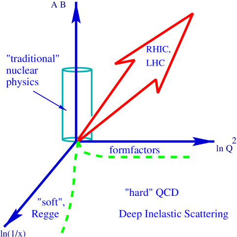
Figure 2: The place of relativistic heavy ion physics in the study of QCD; the vertical axis is the product of atomic numbers of projectile and target, and the horizontal axes are the momentum transfer $Q^{2}$ and rapidity $y=\ln(1/x)$ ($x$ is the Bjorken scaling variable).

It has been conjectured long time ago that the dynamics of QCD in the high density domain may become qualitatively different: in parton language, this is best described in terms of parton saturation [Gribov, Levin and Ryskin (1983), Mueller and Qiu (1986), Blaizot and Mueller (1987)], and in the language of color fields – in terms of the classical Chromo–Dynamics [McLerran and Venugopalan (1994)]; see the lectures [Iancu, Leonidov, McLerran (2002)] and [Mueller (2001)] and references therein. In this high density regime, the transition amplitudes are dominated not by quantum fluctuations, but by the configurations of classical field containing large, $\sim 1/\alpha_{s}$, numbers of gluons. One thus uncovers new non–linear features of QCD, which cannot be investigated in the more traditional applications based on the perturbative approach. The classical color fields in the initial nuclei (the “color glass condensate” [Iancu, Leonidov, McLerran (2002)]) can be thought of as either perturbatively generated, or as being a topologically non–trivial superposition of the Weizsäcker-Williams radiation and the quasi–classical vacuum fields [Kharzeev, Kovchegov and Levin (2001), Nowak, Shuryak and Zahed (2001), Kharzeev, Kovchegov and Levin (2002)].

3.1 Geometrical arguments

Let us consider an external probe $J$ interacting with the nuclear target of atomic number $A$. At small values of Bjorken $x$, by uncertainty principle the interaction develops over large longitudinal distances $z\sim 1/mx$, where $m$ is the nucleon mass. As soon as $z$ becomes larger than the nuclear diameter, the probe cannot distinguish between the nucleons located on the front and back edges of the nucleus, and all partons within the transverse area $\sim 1/Q^{2}$ determined by the momentum transfer $Q$ participate in the interaction coherently. The density of partons in the transverse plane is given by

$$\rho_{A}\simeq{xG_{A}(x,Q^{2})\over\pi R_{A}^{2}}\sim A^{1/3},$$ (25)

where we have assumed that the nuclear gluon distribution scales with the number of nucleons $A$. The probe interacts with partons with cross section $\sigma\sim\alpha_{s}/Q^{2}$; therefore, depending on the magnitude of momentum transfer $Q$, atomic number $A$, and the value of Bjorken $x$, one may encounter two regimes:

• $\sigma\rho_{A}\ll 1$ – this is a familiar “dilute” regime of incoherent interactions, which is well described by the methods of perturbative QCD;

• $\sigma\rho_{A}\gg 1$ – in this regime, we deal with a dense parton system. Not only do the “leading twist” expressions become inadequate, but also the expansion in higher twists, i.e. in multi–parton correlations, breaks down here.

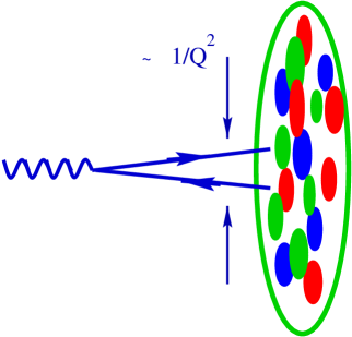
Figure 3: Hard probe interacting with the nuclear target resolves the transverse distance $\sim 1/\sqrt{Q}$ ($Q^{2}$ is the square of the momentum transfer) and, in the target rest frame, the longitudinal distance $\sim 1/(mx)$ ($m$ is the nucleon mass and $x$ – Bjorken variable).

The border between the two regimes can be found from the condition $\sigma\rho_{A}\simeq 1$; it determines the critical value of the momentum transfer (“saturation scale”[Gribov, Levin and Ryskin (1983)]) at which the parton system becomes to look dense to the probe:

$$Q_{s}^{2}\sim\alpha_{s}\ {xG_{A}(x,Q_{s}^{2})\over\pi R_{A}^{2}}.$$ (26)

In this regime, the number of gluons from (26) is given by

$$xG_{A}(x,Q_{s}^{2})\sim{\pi\over\alpha_{s}(Q_{s}^{2})}\ Q_{s}^{2}R_{A}^{2},$$ (27)

where $Q_{s}^{2}R_{A}^{2}\sim A$. One can see that the number of gluons is proportional to the inverse of $\alpha_{s}(Q_{s}^{2})$, and becomes large in the weak coupling regime. In this regime, as we shall now discuss, the dynamics is likely to become essentially classical.

3.2 Saturation as the classical limit of QCD

Indeed, the condition (26) can be derived in the following, rather general, way. As a first step, let us re-scale the gluon fields in the Lagrangian (1) as follows: $A_{\mu}^{a}\to\tilde{A}_{\mu}^{a}=gA_{\mu}^{a}$. In terms of new fields, $\tilde{G}_{\mu\nu}^{a}=gG_{\mu\nu}^{a}=\partial_{\mu}\tilde{A}_{\nu}^{a}-\partial_{\nu}\tilde{A}_{\mu}^{a}+f^{abc}\tilde{A}_{\mu}^{b}\tilde{A}_{\nu}^{c}$, and the dependence of the action corresponding to the Lagrangian (1) on the coupling constant is given by

$$S\sim\int{1\over g^{2}}\ \tilde{G}_{\mu\nu}^{a}\tilde{G}_{\mu\nu}^{a}\ d^{4}x.$$ (28)

Let us now consider a classical configuration of gluon fields; by definition, $\tilde{G}_{\mu\nu}^{a}$ in such a configuration does not depend on the coupling, and the action is large, $S\gg\hbar$. The number of quanta in such a configuration is then

$$N_{g}\sim{S\over\hbar}\sim{1\over\hbar\ g^{2}}\ \rho_{4}V_{4},$$ (29)

where we re-wrote (28) as a product of four–dimensional action density $\rho_{4}$ and the four–dimensional volume $V_{4}$.

Note that since (29) depends only on the product of the Planck constant $\hbar$ and the coupling $g^{2}$, the classical limit $\hbar\to 0$ is indistinguishable from the weak coupling limit $g^{2}\to 0$. The weak coupling limit of small $g^{2}=4\pi\alpha_{s}$ therefore corresponds to the semi–classical regime.

The effects of non–linear interactions among the gluons become important when $\partial_{\mu}\tilde{A}_{\mu}\sim\tilde{A}_{\mu}^{2}$ (this condition can be made explicitly gauge invariant if we derive it from the expansion of a correlation function of gauge-invariant gluon operators, e.g., $\tilde{G}^{2}$). In momentum space, this equality corresponds to

$$Q_{s}^{2}\sim\tilde{A}^{2}\sim(\tilde{G}^{2})^{1/2}=\sqrt{\rho_{4}};$$ (30)

$Q_{s}$ is the typical value of the gluon momentum below which the interactions become essentially non–linear.

Consider now a nucleus $A$ boosted to a high momentum. By uncertainty principle, the gluons with transverse momentum $Q_{s}$ are extended in the longitudinal and proper time directions by $\sim 1/Q_{s}$; since the transverse area is $\pi R_{A}^{2}$, the four–volume is $V_{4}\sim\pi R_{A}^{2}/Q_{s}^{2}$. The resulting four–density from (29) is then

$$\rho_{4}\sim\alpha_{s}\ {N_{g}\over V_{4}}\sim\alpha_{s}\ {N_{g}\ Q_{s}^{2}\over\pi R_{A}^{2}}\sim Q_{s}^{4},$$ (31)

where at the last stage we have used the non–linearity condition (30), $\rho_{4}\sim Q_{s}^{4}$. It is easy to see that (31) coincides with the saturation condition (26), since the number of gluons in the infinite momentum frame $N_{g}\sim xG(x,Q_{s}^{2})$.

In view of the significance of saturation criterion for the rest of the material in these lectures, let us present yet another argument, traditionally followed in the discussion of classical limit in electrodynamics [Berestetskii,Lifshitz and Pitaevskii (1982)]. The energy of the gluon field per unit volume is $\sim\vec{E}^{a2}$. The number of elementary “oscillators of the field”, also per unit volume, is $\sim\omega^{3}$. To get the number of the quanta in the field we have to divide the energy of the field by the product of the number of the oscillators $\sim\omega^{3}$ and the average energy $\hbar\omega$ of the gluon:

$$N_{{\vec{k}}}\sim{\vec{E}^{a2}\over\hbar\omega^{4}}.$$ (32)

The classical approximation holds when $N_{{\vec{k}}}\gg 1$. Since the energy $\omega$ of the oscillators is related to the time $\Delta t$ over which the average energy is computed by $\omega\sim 1/\Delta t$, we get

$$\vec{E}^{a2}\gg{\hbar\over(\Delta t)^{4}}.$$ (33)

Note that the quantum mechanical uncertainty principle for the energy of the field reads

$$\vec{E}^{a2}\ \omega^{4}\sim\hbar,$$ (34)

so the condition (33) indeed defines the quasi–classical limit.

Since $\vec{E}^{a2}$ is proportional to the action density $\rho_{4}$, and the typical time is $\Delta t\sim 1/k_{\perp}$, using (31) we finally get that the classical description applies when

$$k_{\perp}^{2}<\alpha_{s}{N_{g}\over\pi R_{A}^{2}}\equiv Q_{s}^{2}.$$ (35)

3.3 The absence of mini–jet correlations

When the occupation numbers of the field become large, the matrix elements of the creation and annihilation operators of the gluon field defined by

$$\hat{A}^{\mu}=\sum_{\vec{k},\alpha}(\hat{c}_{\vec{k}\alpha}A^{\mu}_{\vec{k}\alpha}+\hat{c}^{\dagger}_{\vec{k}\alpha}A^{\mu*}_{\vec{k}\alpha})$$ (36)

become very large,

$$N_{\vec{k}\alpha}=\langle\hat{c}^{\dagger}_{\vec{k}\alpha}\hat{c}_{\vec{k}\alpha}\rangle\gg 1,$$ (37)

so that one can neglect the unity on the r.h.s. of the commutation relation

$$\hat{c}_{\vec{k}\alpha}\hat{c}^{\dagger}_{\vec{k}\alpha}-\hat{c}^{\dagger}_{\vec{k}\alpha}\hat{c}_{\vec{k}\alpha}=1$$ (38)

and treat these operators as classical $c-$numbers.

This observation, often used in condensed matter physics, especially in the theoretical treatment of superfluidity, has important consequences for gluon production – in particular, it implies that the correlations among the gluons in the saturation region can be neglected:

$$\langle A(k_{1})A(k_{2})...A(k_{n})\rangle\simeq\langle A(k_{1})\rangle\langle A(k_{2})\rangle...\langle A(k_{n})\rangle.$$ (39)

Thus, in contrast to the perturbative picture, where the produced mini-jets have strong back-to-back correlations, the gluons resulting from the decay of the classical saturated field are uncorrelated at $k_{\perp}\lsim Q_{s}$.

Note that the amplitude with the factorization property (39) is called point–like. However, the relation (39) cannot be exact if we consider the correlations of final–state hadrons – the gluon mini–jets cannot transform into hadrons independently. These correlations caused by color confinement however affect mainly hadrons with close three–momenta, as opposed to the perturbative correlations among mini–jets with the opposite three–momenta.

It will be interesting to explore the consequences of the factorization property of the classical gluon field (39) for the HBT correlations of final–state hadrons. It is likely that the HBT radii in this case reflect the universal color correlations in the hadronization process.

Another interesting property of classical fields follows from the relation

$$\langle(\hat{c}^{\dagger}_{\vec{k}\alpha}\hat{c}_{\vec{k}\alpha})^{2}\rangle-\langle\hat{c}^{\dagger}_{\vec{k}\alpha}\hat{c}_{\vec{k}\alpha}\rangle^{2}=\langle\hat{c}^{\dagger}_{\vec{k}\alpha}\hat{c}_{\vec{k}\alpha}\rangle,$$ (40)

which determines the fluctuations in the number of produced gluons. We will discuss the implications of Eq. (40) for the multiplicity fluctuations in heavy ion collisions later.

4 Classical QCD in action

4.1 Centrality dependence of hadron production

In nuclear collisions, the saturation scale becomes a function of centrality; a generic feature of the quasi–classical approach – the proportionality of the number of gluons to the inverse of the coupling constant (29) – thus leads to definite predictions [Kharzeev and Nardi (2001)] on the centrality dependence of multiplicity.

Let us first present the argument on a qualitative level. At different centralities (determined by the impact parameter of the collision), the average density of partons (in the transverse plane) participating in the collision is very different. This density $\rho$ is proportional to the average length of nuclear material involved in the collision, which in turn approximately scales with the power of the number $N_{part}$ of participating nucleons, $\rho\sim N_{part}^{1/3}$. The density of partons defines the value of the saturation scale, and so we expect

$$Q_{s}^{2}\sim N_{part}^{1/3}.$$ (41)

The gluon multiplicity is then, as we discussed above, is

$${dN_{g}\over d\eta}\sim{S_{A}\ Q_{s}^{2}\over\alpha_{s}(Q_{s}^{2})},$$ (42)

where $S_{A}$ is the nuclear overlap area, determined by atomic number and the centrality of collision. Since $S_{A}\ Q_{s}^{2}\sim N_{part}$ by definitions of the transverse density and area, from (42) we get

$${dN_{g}\over d\eta}\sim N_{part}\ \ln N_{part},$$ (43)

which shows that the gluon multiplicity shows a logarithmic deviation from the scaling in the number of participants.

To quantify the argument, we need to explicitly evaluate the average density of partons at a given centrality. This can be done by using Glauber theory, which allows to evaluate the differential cross section of the nucleus–nucleus interactions. The shape of the multiplicity distribution at a given (pseudo)rapidity $\eta$ can then be readily obtained (see, e.g., [Kharzeev, Lourenço, Nardi and Satz (1997)]):

$$\frac{d\sigma}{dn}=\int d^{2}b\ {\cal P}(n;b)\ (1-P_{0}(b)),$$ (44)

where $P_{0}(b)$ is the probability of no interaction among the nuclei at a given impact parameter $b$:

$$P_{0}(b)=(1-\sigma_{NN}T_{AB}(b))^{AB};$$ (45)

$\sigma_{NN}$ is the inelastic nucleon–nucleon cross section, and $T_{AB}(b)$ is the nuclear overlap function for the collision of nuclei with atomic numbers A and B; we have used the three–parameter Woods–Saxon nuclear density distributions [De Jager, De Vries and De Vries (1974)].

The correlation function ${\cal P}(n;b)$ is given by

$${\cal P}(n;b)=\frac{1}{\sqrt{2\pi a\bar{n}(b)}}\ \exp\left(-\frac{(n-\bar{n}(b))^{2}}{2a\bar{n}(b)}\right),$$ (46)

here $\bar{n}(b)$ is the mean multiplicity at a given impact parameter $b$; the formulae for the number of participants and the number of binary collisions can be found in [Kharzeev, Lourenço, Nardi and Satz (1997)]. The parameter $a$ describes the strength of fluctuations; for the classical gluon field, as follows from (40), $a=1$. However, the strength of fluctuations can be changed by the subsequent evolution of the system and by hadronization process. Moreover, in a real experiment, the strength of fluctuations strongly depends on the acceptance. In describing the PHOBOS distribution [PHOBOS Coll. (2000)], we have found that the value $a=0.6$ fits the data well.

In Fig.4, we compare the resulting distributions for two different assumptions about the scaling of multiplicity with the number of participants to the PHOBOS experimental distribution, measured in the interval $3<|\eta|<4.5$. One can see that almost independently of theoretical assumptions about the dynamics of multiparticle production, the data are described quite well. At first this may seem surprising; the reason for this result is that at high energies, heavy nuclei are almost completely “black”; unitarity then implies that the shape of the cross section is determined almost entirely by the nuclear geometry. We can thus use experimental differential cross sections as a reliable handle on centrality. This gives us a possibility to compute the dependence of the saturation scale on centrality of the collision, and thus to predict the centrality dependence of particle multiplicities, shown in Fig. 5. (see [Kharzeev and Nardi (2001)] for details).

Figure 4: Charged multiplicity distribution at $\sqrt{s}=130$ A GeV; solid line (histogram) – PHOBOS result; dashed line – distribution corresponding to participant scaling ($x=0$); dotted line – distribution corresponding to the $37\%$ admixture of “hard” component in the multiplicity; see text for details.

Figure 5: Centrality dependence of the charged multiplicity per participant pair near $\eta=0$ at $\sqrt{s}=130$ A GeV; the curves represent the prediction based on the conventional eikonal approach, while the diamonds correspond to the high density QCD prediction (see text). The square indicates the $pp$ multiplicity.

4.2 Energy dependence

Let us now turn to the discussion of energy dependence of hadron production. In semi–classical scenario, it is determined by the variation of saturation scale $Q_{s}$ with Bjorken $x=Q_{s}/\sqrt{s}$. This variation, in turn, is determined by the $x-$ dependence of the gluon structure function. In the saturation approach, the gluon distribution is related to the saturation scale by Eq.(26). A good description of HERA data is obtained with saturation scale $Q_{s}^{2}=1\div 2\ \rm{GeV}^{2}$ with $W$ - dependence ($W\equiv\sqrt{s}$ is the center-of-mass energy available in the photon–nucleon system) [Golec-Biernat and Wüsthof (1999)]

$$Q^{2}_{s}\,\,\propto\,W^{\lambda},$$ (47)

where $\lambda\simeq 0.25\div 0.3$. In spite of significant uncertainties in the determination of the gluon structure functions, perhaps even more important is the observation [Golec-Biernat and Wüsthof (1999)] that the HERA data exhibit scaling when plotted as a function of variable

$$\tau\,=\,{Q^{2}\over Q_{0}^{2}}\ \left({x\over x_{0}}\right)^{\lambda},$$ (48)

where the value of $\lambda$ is again within the limits $\lambda\simeq 0.25\div 0.3$. In high density QCD, this scaling is a consequence of the existence of dimensionful scale [Gribov, Levin and Ryskin (1983), McLerran and Venugopalan (1994)])

$$Q_{s}^{2}(x)=Q_{0}^{2}\ (x_{0}/x)^{\lambda}.$$ (49)

Using the value of $Q_{s}^{2}\simeq 2.05\ {\rm GeV}^{2}$ extracted [Kharzeev and Nardi (2001)] at $\sqrt{s}=130$ GeV and $\lambda=0.25$ [Golec-Biernat and Wüsthof (1999)] used in [Kharzeev and Levin (2000)], equation (59) leads to the following approximate formula for the energy dependence of charged multiplicity in central $Au-Au$ collisions:

$$\left<{2\over N_{part}}\ {dN_{ch}\over d\eta}\right>_{\eta<1}\approx 0.87\ \left({\sqrt{s}\ ({\rm GeV})\over 130}\right)^{0.25}\ \times$$

$$\times\left[3.93+0.25\ \ln\left({\sqrt{s}\ ({\rm GeV})\over 130}\right)\right].$$ (50)

At $\sqrt{s}=130\ {\rm GeV}$, we estimate from Eq.(50) $2/N_{part}\ dN_{ch}/d\eta\mid_{\eta<1}=3.42\pm 0.15$, to be compared to the average experimental value of $3.37\pm 0.12$ [PHOBOS Coll. (2000), PHENIX Coll. (2001), STAR Coll. (2001), BRAHMS Coll. (2001)]. At $\sqrt{s}=200\ {\rm GeV}$, one gets $3.91\pm 0.15$, to be compared to the PHOBOS value [PHOBOS Coll. (2000)] of $3.78\pm 0.25$. Finally, at $\sqrt{s}=56\ {\rm GeV}$, we find $2.62\pm 0.15$, to be compared to [PHOBOS Coll. (2000)] $2.47\pm 0.25$. It is interesting to note that formula (50), when extrapolated to very high energies, predicts for the LHC energy a value substantially smaller than found in other approaches:

$$\left<{2\over N_{part}}\ {dN_{ch}\over d\eta}\right>_{\eta<1}=10.8\pm 0.5;\ \ \ \sqrt{s}=5500\ {\rm GeV},$$ (51)

corresponding only to a factor of $2.8$ increase in multiplicity between the RHIC energy of $\sqrt{s}=200\ {\rm GeV}$ and the LHC energy of $\sqrt{s}=5500\ {\rm GeV}$ (numerical calculations show that when normalized to the number of participants, the multiplicity in central $Au-Au$ and $Pb-Pb$ systems is almost identical). The energy dependence of charged hadron multiplicity per participant pair is shown in Fig.6.

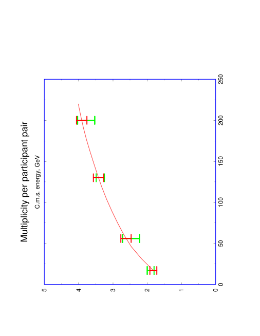
Figure 6: Energy dependence of charged multiplicity per participant pair at RHIC energies; solid line is the result (50).

One can also try to extract the value of the exponent $\lambda$ from the energy dependence of hadron multiplicity measured by PHOBOS at $\sqrt{s}=130\ \rm{GeV}$ and at at $\sqrt{s}=56\ \rm{GeV}$; this procedure yields $\lambda\simeq 0.37$, which is larger than the value inferred from the HERA data (and is very close to the value $\lambda\simeq 0.38$, resulting from the final–state saturation calculations [Eskola, Kajantie, Ruuskanen and Tuominen (2000)]).

4.3 Radiating the classical glue

Let us now proceed to the quantitative calculation of the (pseudo-) rapidity and centrality dependences [Kharzeev and Levin (2001)]. We need to evaluate the leading tree diagram describing emission of gluons on the classical level, see Fig. 7.

Figure 7: The Mueller diagram for the classical gluon radiation.

Let us introduce the unintegrated gluon distribution $\varphi_{A}(x,k_{t}^{2})$ which describes the probability to find a gluon with a given $x$ and transverse momentum $k_{t}$ inside the nucleus $A$. As follows from this definition, the unintegrated distribution is related to the gluon structure function by

$$xG_{A}(x,p_{t}^{2})=\int^{p_{t}^{2}}dk_{t}^{2}\ \varphi_{A}(x,k_{t}^{2});$$ (52)

when $p_{t}^{2}>Q_{s}^{2}$, the unintegrated distribution corresponding to the bremsstrahlung radiation spectrum is

$$\varphi_{A}(x,k_{t}^{2})\sim{\alpha_{s}\over\pi}\ {1\over k_{t}^{2}}.$$ (53)

In the saturation region, the gluon structure function is given by (27); the corresponding unintegrated gluon distribution has only logarithmic dependence on the transverse momentum:

$$\varphi_{A}(x,k_{t}^{2})\sim{S_{A}\over\alpha_{s}};\ k_{t}^{2}\leq Q_{s}^{2},$$ (54)

where $S_{A}$ is the nuclear overlap area, determined by the atomic numbers of the colliding nuclei and by centrality of the collision.

The differential cross section of gluon production in a $AA$ collision can now be written down as [Gribov, Levin and Ryskin (1983), Gyulassy and McLerran (1997)]

$$E{d\sigma\over d^{3}p}={4\pi N_{c}\over N_{c}^{2}-1}\ {1\over p_{t}^{2}}\ \int dk_{t}^{2}\ \alpha_{s}\ \varphi_{A}(x_{1},k_{t}^{2})\ \varphi_{A}(x_{2},(p-k)_{t}^{2}),$$ (55)

where $x_{1,2}=(p_{t}/\sqrt{s})\exp(\pm\eta)$, with $\eta$ the (pseudo)rapidity of the produced gluon; the running coupling $\alpha_{s}$ has to be evaluated at the scale $Q^{2}=max\{k_{t}^{2},(p-k)_{t}^{2}\}$. The rapidity density is then evaluated from (55) according to

$${dN\over dy}={1\over\sigma_{AA}}\ \int d^{2}p_{t}\left(E{d\sigma\over d^{3}p}\right),$$ (56)

where $\sigma_{AA}$ is the inelastic cross section of nucleus–nucleus interaction.

Since the rapidity $y$ and Bjorken variable are related by $\ln 1/x=y$, the $x-$ dependence of the gluon structure function translates into the following dependence of the saturation scale $Q_{s}^{2}$ on rapidity:

$$Q_{s}^{2}(s;\pm y)=Q_{s}^{2}(s;y=0)\ \exp(\pm\lambda y).$$ (57)

As it follows from (57), the increase of rapidity at a fixed $W\equiv\sqrt{s}$ moves the wave function of one of the colliding nuclei deeper into the saturation region, while leading to a smaller gluon density in the other, which as a result can be pushed out of the saturation domain. Therefore, depending on the value of rapidity, the integration over the transverse momentum in Eqs. (55),(56) can be split in two regions: i) the region $\Lambda_{QCD}<k_{t}<Q_{s,min}$ in which the wave functions are both in the saturation domain; and ii) the region $\Lambda<<Q_{s,min}<k_{t}<Q_{s,max}$ in which the wave function of one of the nuclei is in the saturation region and the other one is not. Of course, there is also the region of $k_{t}>Q_{s,max}$, which is governed by the usual perturbative dynamics, but our assumption here is that the rôle of these genuine hard processes in the bulk of gluon production is relatively small; in the saturation scenario, these processes represent quantum fluctuations above the classical background. It is worth commenting that in the conventional mini–jet picture, this classical background is absent, and the multi–particle production is dominated by perturbative processes. This is the main physical difference between the two approaches; for the production of particles with $p_{t}>>Q_{s}$ they lead to identical results.

To perform the calculation according to (56),(55) away from $y=0$ we need also to specify the behavior of the gluon structure function at large Bjorken $x$ (and out of the saturation region). At $x\to 1$, this behavior is governed by the QCD counting rules, $xG(x)\sim(1-x)^{4}$, so we adopt the following conventional form: $xG(x)\sim x^{-\lambda}\ (1-x)^{4}$.

We now have everything at hand to perform the integration over transverse momentum in (56), (55); the result is the following [Kharzeev and Levin (2001)]:

$${dN\over dy}=const\ S_{A}\ Q_{s,min}^{2}\ \ln\left({Q_{s,min}^{2}\over\Lambda_{QCD}^{2}}\right)\ \times$$

$$\times\ \left[1+{1\over 2}\ \ln\left({Q_{s,max}^{2}\over Q_{s,min}^{2}}\right)\ \left(1-{Q_{s,max}\over\sqrt{s}}e^{|y|}\right)^{4}\right],$$ (58)

where the constant is energy–independent, $S_{A}$ is the nuclear overlap area, $Q_{s}^{2}\equiv Q_{s}^{2}(s;y=0)$, and $Q_{s,min(max)}$ are defined as the smaller (larger) values of (57); at $y=0$, $Q_{s,min}^{2}=Q_{s,max}^{2}=Q_{s}^{2}(s)=Q_{s}^{2}(s_{0})\ \times$ $\times(s/s_{0})^{\lambda/2}$. The first term in the brackets in (58) originates from the region in which both nuclear wave functions are in the saturation regime; this corresponds to the familiar $\sim(1/\alpha_{s})\ Q_{s}^{2}R_{A}^{2}$ term in the gluon multiplicity. The second term comes from the region in which only one of the wave functions is in the saturation region. The coefficient $1/2$ in front of the second term in square brackets comes from $k_{t}$ ordering of gluon momenta in evaluation of the integral of Eq.(55).

The formula (58) has been derived using the form (54) for the unintegrated gluon distributions. We have checked numerically that the use of more sophisticated functional form of $\varphi_{A}$ taken from the saturation model of Golec-Biernat and Wüsthoff [Golec-Biernat and Wüsthof (1999)] in Eq.(55) affects the results only at the level of about $3\%$.

Since $S_{A}Q_{s}^{2}\sim N_{part}$ (recall that $Q_{s}^{2}\gg\Lambda_{QCD}^{2}$ is defined as the density of partons in the transverse plane, which is proportional to the density of participants), we can re–write (58) in the following final form [Kharzeev and Levin (2001)]

$${dN\over dy}=c\ N_{part}\ \left({s\over s_{0}}\right)^{\lambda\over 2}\ e^{-\lambda|y|}\ \left[\ln\left({Q_{s}^{2}\over\Lambda_{QCD}^{2}}\right)-\lambda|y|\right]\ \times$$

$$\times\left[1+\lambda|y|\left(1-{Q_{s}\over\sqrt{s}}\ e^{(1+\lambda/2)|y|}\right)^{4}\right],$$ (59)

with $Q_{s}^{2}(s)=Q_{s}^{2}(s_{0})\ (s/s_{0})^{\lambda/2}$. This formula is the central result of our paper; it expresses the predictions of high density QCD for the energy, centrality, rapidity, and atomic number dependences of hadron multiplicities in nuclear collisions in terms of a single scaling function. Once the energy–independent constant $c\sim 1$ and $Q_{s}^{2}(s_{0})$ are determined at some energy $s_{0}$, Eq. (59) contains no free parameters. At $y=0$ the expression (58) coincides exactly with the one derived in [Kharzeev and Nardi (2001)], and extends it to describe the rapidity and energy dependences.

4.4 Converting gluons into hadrons

The distribution (59) refers to the radiated gluons, while what is measured in experiment is, of course, the distribution of final hadrons. We thus have to make an assumption about the transformation of gluons into hadrons. The gluon mini–jets are produced with a certain virtuality, which changes as the system evolves; the distribution in rapidity is thus not preserved. However, in the analysis of jet structure it has been found that the angle of the produced gluon is remembered by the resulting hadrons; this property of “local parton–hadron duality” (see [Dokshitzer (1998)] and references therein) is natural if one assumes that the hadronization is a soft process which cannot change the direction of the emitted radiation. Instead of the distribution in the angle $\theta$, it is more convenient to use the distribution in pseudo–rapidity $\eta=-\ln\tan(\theta/2)$. Therefore, before we can compare (58) to the data, we have to convert the rapidity distribution (59) into the gluon distribution in pseudo–rapidity. We will then assume that the gluon and hadron distributions are dual to each other in the pseudo–rapidity space.

To take account of the difference between rapidity $y$ and the measured pseudo-rapidity $\eta$, we have to multiply (58) by the Jacobian of the $y\leftrightarrow\eta$ transformation; a simple calculation yields

$$h(\eta;p_{t};m)=\frac{\cosh\eta}{\sqrt{\frac{m^{2}\,+\,p_{t}^{2}}{p_{t}^{2}}\,\,+\,\,\sinh^{2}\eta}},$$ (60)

where $m$ is the typical mass of the produced particle, and $p_{t}$ is its typical transverse momentum. Of course, to plot the distribution (59) as a function of pseudo-rapidity, one also has to express rapidity $y$ in terms of pseudo-rapidity $\eta$; this relation is given by

$$y(\eta;p_{t};m)={1\over 2}\ \ln\left[{{\sqrt{\frac{m^{2}\,+\,p_{t}^{2}}{p_{t}^{2}}\,\,+\,\,\sinh^{2}\eta}}+\sinh\eta}\over{{\sqrt{\frac{m^{2}\,+\,p_{t}^{2}}{p_{t}^{2}}\,\,+\,\,\sinh^{2}\eta}}-\sinh\eta}\right];$$ (61)

obviously, $h(\eta;p_{t};m)={\partial y(\eta;p_{t};m)/\partial\eta}$.

We now have to make an assumption about the typical invariant mass $m$ of the gluon mini–jet. Let us estimate it by assuming that the slowest hadron in the mini-jet decay is the $\rho$-resonance, with energy $E_{\rho}=(m_{\rho}^{2}+p_{\rho,t}^{2}+p_{\rho,z}^{2})^{1/2}$, where the $z$ axis is pointing along the mini-jet momentum. Let us also denote by $x_{i}$ the fractions of the gluon energy $q_{0}$ carried by other, fast, $i$ particles in the mini-jet decay. Since the sum of transverse (with respect to the mini-jet axis) momenta of mini-jet decay products is equal to zero, the mini-jet invariant mass $m$ is given by

$$m^{2}_{jet}\,\equiv\,m^{2}=(\sum_{i}x_{i}q_{0}+E_{\rho})^{2}-(\sum_{i}x_{i}q_{z}+p_{\rho,z})^{2}\,\simeq\,\,$$

$$\,\simeq\,\,2\sum_{i}x_{i}q_{z}\cdot(m_{\rho,t}-p_{\rho,z})\equiv 2Q_{s}\cdot m_{eff},$$ (62)

where $m_{\rho,t}=(m_{\rho}^{2}+p_{\rho,t}^{2})^{1/2}$. In Eq. (62) we used that $\sum_{i}x_{i}=1$ and $q_{0}\approx q_{z}=Q_{s}$. Taking $p_{\rho,z}\approx p_{\rho,t}\approx\,300$ MeV and $\rho$ mass, we obtain $m_{eff}\approx 0.5\,$ GeV.

We thus use the mass $m^{2}\simeq 2Q_{s}m_{eff}\simeq Q_{s}\cdot 1$ GeV in Eqs.(60,61). Since the typical transverse momentum of the produced gluon mini–jet is $Q_{s}$, we take $p_{t}=Q_{s}$ in (60). The effect of the transformation from rapidity to pseudo–rapidity is the decrease of multiplicity at small $\eta$ by about $25-30\%$, leading to the appearance of the $\approx 10\%$ dip in the pseudo–rapidity distribution in the vicinity of $\eta=0$. We have checked that the change in the value of the mini–jet mass by two times affects the Jacobian at central pseudo–rapidity to about $\simeq 10\%$, leading to $\sim 3\%$ effect on the final result.

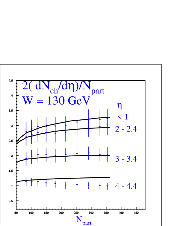
Figure 8: Centrality dependence of charged hadron production per participant at different pseudo-rapidity $\eta$ intervals in $Au-Au$ collisions at $\sqrt{s}=130$ GeV; from (Kharzeev and Levin, 2001), the data are from (PHOBOS Coll., 2000).

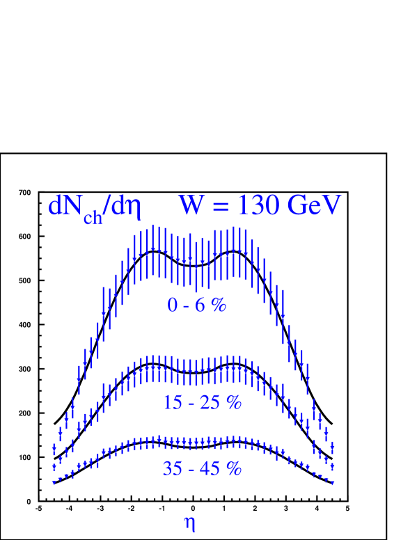
Figure 9: Pseudo–rapidity dependence of charged hadron production at different cuts on centrality in $Au-Au$ collisions at $\sqrt{s}=130$ GeV; from (Kharzeev and Levin, 2001), the data are from (PHOBOS Coll., 2000).

The results for the $Au-Au$ collisions at $\sqrt{s}=130$ GeV are presented in Figs 8 and 9. In the calculation, we use the results on the dependence of saturation scale on the mean number of participants at $\sqrt{s}=130$ GeV from [Kharzeev and Nardi (2001)], see Table 2 of that paper. The mean number of participants in a given centrality cut is taken from the PHOBOS paper [PHOBOS Coll. (2000)]. One can see that both the centrality dependence and the rapidity dependence of the $\sqrt{s}=130$ GeV PHOBOS data are well reproduced below $\eta\simeq\pm 4$. The rapidity dependence has been evaluated with $\lambda=0.25$, which is within the range $\lambda=0.25\div 0.3$ inferred from the HERA data [Golec-Biernat and Wüsthof (1999)]. The discrepancy above $\eta\simeq\pm 4$ is not surprising since our approach does not properly take into account multi–parton correlations which are important in the fragmentation region.

Our predictions for $Au-Au$ collisions at $\sqrt{s}=200$ GeV are presented in [Kharzeev and Levin (2001)]. The only parameter which governs the energy dependence is the exponent $\lambda$, which we assume to be $\lambda\simeq 0.25$ as inferred from the HERA data. The absolute prediction for the multiplicity, as explained above, bears some uncertainty, but there is a definite feature of our scenario which is distinct from other approaches. It is the dependence of multiplicity on centrality, which around $\eta=0$ is determined solely by the running of the QCD strong coupling [Kharzeev and Nardi (2001)]. As a result, the centrality dependence at $\sqrt{s}=200$ GeV is somewhat less steep than at $\sqrt{s}=130$. While the difference in the shape at these two energies is quite small, in the perturbative mini-jet picture this slope should increase, reflecting the growth of the mini-jet cross section with energy [Wang and Gyulassy (2001)].

4.5 Further tests

Checking the predictions of the semi–classical approach for the centrality and pseudo–rapidity dependence at $\sqrt{s}=200$ GeV is clearly very important. What other tests of this picture can one devise? The main feature of the classical emission is that it is coherent up to the transverse momenta of about $\sqrt{2}\ Q_{s}$ (about $\simeq 2$ GeV/c for central $Au-Au$ collisions). This means that if we look at the centrality dependence of particle multiplicities above a certain value of the transverse momentum, say, above $1$ GeV/c, it should be very similar to the dependence without the transverse momentum cut-off. On the other hand, in the two–component “soft plus hard” model the cut on the transverse momentum would strongly enhance the contribution of hard mini–jet production processes, since soft production mechanisms presumably do not contribute to particle production at high transverse momenta. Of course, at sufficiently large value of the cutoff all of the observed particles will originate from genuine hard processes, and the centrality dependence will become steeper, reflecting the scaling with the number of collisions. It will be very interesting to explore the transition to this hard scattering regime experimentally.

Another test, already discussed above (see eq.(39)) is the study of azimuthal correlations between the produced high $p_{t}$ particles. In the saturation scenario these correlations should be very small below $p_{t}\simeq 2$ GeV/c in central collisions. At higher transverse momenta, and/or for more peripheral collisions (where the saturation scale is smaller) these correlations should be much stronger.

5 Does the vacuum melt?

The approach described above allows us to estimate the initial energy density of partons achieved at RHIC. Indeed, in this approach the formation time of partons is $\tau_{0}\simeq 1/Q_{s}$, and the transverse momenta of partons are about $k_{t}\simeq Q_{s}$. We thus can use the Bjorken formula and the set of parameters deduced above to estimate [Kharzeev and Nardi (2001)]

$$\epsilon\simeq{<k_{t}>\over\tau_{0}}\ {d^{2}N\over d^{2}bd\eta}\simeq Q_{s}^{2}\ {d^{2}N\over d^{2}bd\eta}\simeq 18\ {\rm{GeV/fm^{3}}}$$ (63)

for central $Au-Au$ collisions at $\sqrt{s}=130$ GeV. This value is well above the energy density needed to induce the QCD phase transition according to the lattice calculations. However, the picture of gluon production considered above seems to imply that the gluons simply flow from the initial state of the incident nuclei to the final state, where they fragment into hadrons, with nothing spectacular happening on the way. In fact, one may even wonder if the presence of these gluons modifies at all the structure of the physical QCD vacuum.

To answer this question theoretically, we have to possess some knowledge about the non–perturbative vacuum properties. While in general the problem of vacuum structure still has not been solved (and this is one of the main reasons for the heavy ion research!), we do know one class of vacuum solutions – the instantons. It is thus interesting to investigate what happens to the QCD vacuum in the presence of strong external classical fields using the example of instantons [Kharzeev, Kovchegov and Levin (2002)].

Figure 10: Distributions of instanton sizes in vacuum for QCD with three light flavors (upper curve) versus the distribution of instanton sizes in the saturation environment produced by a collision of two identical nuclei for $c=1$ (middle curve) and $c=2\ln 2$ (lower curve) with $Q_{s}^{2}\,=\,2\,\mbox{GeV}^{2}$; from (Kharzeev, Kovchegov and Levin, 2002).

The problem of small instantons in a slowly varying background field was first addressed in [Callan, Dashen and Gross (1979), Shifman, Vainshtein and Zakharov (1980)] by introducing the effective instanton lagrangian $L^{I(\overline{I})}_{eff}(x)$

$$L_{eff}^{I}(x_{0})\,=\,\int d\rho\,n_{0}(\rho)\,dR\,\exp\left(-\frac{2\pi^{2}}{g}\,\rho^{2}\,\overline{\eta}^{M}_{a\mu\nu}\,R^{aa^{\prime}}\,G^{a^{\prime}}_{\mu\nu}(x_{0})\right)$$ (64)

in which $n_{0}(\rho)$ is the instanton size distribution function in the vacuum, $\overline{\eta}^{M}_{a\mu\nu}$ is the ’t Hooft symbol in Minkowski space, and $R^{aa^{\prime}}$ is the matrix of rotations in color space, with $dR$ denoting the averaging over the instanton color orientations.

The complete field of a single instanton solution could be reconstructed by perturbatively resumming the powers of the effective instanton lagrangian which corresponds to perturbation theory in powers of the instanton size parameter $\rho^{2}$. In our case here the background field arises due to the strong source current $J_{\mu}^{a}$. The current can be due to a single nucleus, or resulting from the two colliding nuclei. Perturbative resummation of powers of the source current term translates itself into resummation of the powers of the classical field parameter $\alpha_{s}^{2}A^{1/3}$ [McLerran and Venugopalan (1994), Kovchegov (1996)]. Thus the problem of instantons in the background classical gluon field is described by the effective action in Minkowski space

$$S_{eff}\,=\,\int d^{4}x\left(-\frac{1}{4}G^{a}_{\mu\nu}(x)G^{a}_{\mu\nu}(x)\,+\,L^{I}_{eff}(x)\,+\,L^{\overline{I}}_{eff}(x)\,+\,J_{\mu}^{a}\,A_{\mu}^{a}(x)\right).$$ (65)

The problem thus is clearly formulated; by using an explicit form for the radiated classical gluon field, it was possible to demonstrate [Kharzeev, Kovchegov and Levin (2002)] that the distribution of instantons gets modified from the original vacuum one $n_{0}(\rho)$ to

$$n_{sat}^{AA}(\rho)\,=\,n_{0}(\rho)\,\exp\left(-\frac{c\,\rho^{4}Q_{s}^{4}}{8\,\alpha_{s}^{2}\,N_{c}\,(Q_{s}\tau_{0})^{2}}\right),$$ (66)

where $\tau_{0}$ is the proper time. The result Eq. (66) shows that large size instantons are suppressed by the strong classical fields generated in the nuclear collision (see Fig. 10). The vacuum does melt!

The results presented here were obtained together with Hirotsugu Fujii, Yuri Kovchegov, Eugene Levin, and Marzia Nardi. I am very grateful to them for the most enjoyable collaboration. I also wish to thank Jean-Paul Blaizot, Yuri Dokshitzer, Larry McLerran, Al Mueller and Raju Venugopalan for numerous illuminating discussions on the subject of these lectures. This work was supported by the U.S. Department of Energy under Contract No. DE-AC02-98CH10886.

References

- PHENIX Coll. (2001) Adcox, K. et al., (The PHENIX Collaboration), Phys. Rev. Lett. 86:3500, 2001; Phys. Rev. Lett. 87:052301, 2001; Milov, A. et al., (The PHENIX Collaboration), nucl-ex/0107006.
- STAR Coll. (2001) Adler, C. et al., (The STAR Collaboration), Phys. Rev. Lett. 87:112303, 2001; Phys. Rev. Lett. 87:082301, 2001.
- Anselm and Gribov (1972) Anselm, A.A. and Gribov, V.N., Physics Letters B40:487, 1972.
- PHOBOS Coll. (2000) Back, B. et al., PHOBOS Coll., Phys. Rev. Lett. 85:3100, 2000; Phys. Rev. Lett. 87:102303, 2001; nucl-ex/0105011; nucl-ex/0108009.
- BRAHMS Coll. (2001) Bearden I.G. et al., (The BRAHMS Collaboration), Phys. Rev. Lett. 87:112305, 2001; nucl-ex/0102011; nucl-ex/0108016
- Berestetskii,Lifshitz and Pitaevskii (1982) Berestetskii, V. B., Lifshitz, E.M. and Pitaevskii, L.P., “Quantum electrodynamics”, Oxford New York, Pergamon Press, 1982.
- Blaizot and Mueller (1987) Blaizot, J.P. and Mueller, A.H., Nucl. Phys. B289:847, 1987.
- Callan, Dashen and Gross (1979) Callan, C.G., Dashen, R. and Gross, D.J., Phys. Rev. D19:1826, 1979.
- Casimir and Polder (1948) Casimir, H.B.G. and Polder, D., Phys. Rev. 73:360, 1948.
- De Jager, De Vries and De Vries (1974) De Jager, C., De Vries, H. and De Vries, C., Atom. Nucl. Data Tabl. 14:479, 1974.
- Dokshitzer (1998) Dokshitzer, Yu.L., hep-ph/9801372.
- Dokshitzer (1998) Dokshitzer, Yu.L., hep-ph/9812252.
-
Eskola, Kajantie, Ruuskanen and Tuominen (2000)
Eskola, K.J., Kajantie, K. and Tuominen, K., Phys. Lett. B497:39, 2001;
Eskola, K.J., Kajantie, K., Ruuskanen, P.V. and Tuominen, K., Nucl. Phys. B 570:379, 2000. - Fujii and Kharzeev (1999) Fujii, H. and Kharzeev, D., Phys. Rev. D60:114039, 1999; hep-ph/9807383.
- Golec-Biernat and Wüsthof (1999) Golec-Biernat, K. and Wüsthof, M., Phys. Rev. D59:014017, 1999; Phys. Rev. D60:114023, 1999; Stasto, A., Golec-Biernat, K. and Kwiecinski, J., Phys. Rev. Lett. 86:596, 2001.
- Gribov (1999) Gribov, V.N., Eur. Phys. J. C10:71; 91, 1999.
- Gribov, Levin and Ryskin (1983) Gribov, L.V., Levin, E.M. and Ryskin, M.G., Phys. Rept. 100:1, 1983.
-
Gross and Wilczek; Politzer (1973)
Gross, D.J., and Wilczek, F., Phys. Rev. Lett. 30:1343, 1973;
Politzer, H.D., Phys. Rev. Lett. 30:1346, 1973. - Gyulassy and McLerran (1997) Gyulassy, M. and McLerran, L., Phys. Rev. C56:2219, 1997.
- Iancu, Leonidov, McLerran (2002) Iancu, I., Leonidov, A., and McLerran, L. hep-ph/0202270.
- Kharzeev and Levin (2000) Kharzeev, D. and Levin, E., Nucl. Phys. B578:351, 2000.
- Kharzeev and Nardi (2001) Kharzeev, D. and Nardi, Phys. Lett. B507:121, 2001.
- Kharzeev and Levin (2001) Kharzeev, D. and Levin, E., Phys. Lett. B523:79, 2001.
- Kharzeev, Kovchegov and Levin (2001) Kharzeev, D., Kovchegov, Yu. and Levin, E., Nucl. Phys. A690:621, 2001;
- Kharzeev, Kovchegov and Levin (2002) Kharzeev, D., Kovchegov, Yu. and Levin, E., Nucl.Phys.A699:745, 2002.
- Kharzeev, Lourenço, Nardi and Satz (1997) Kharzeev, D., Lourenço, C., Nardi, M. and Satz, H., Z.Phys. C74:307, 1997.
- Kharzeev (1996) Kharzeev, D. Quarkonium Interactions in QCD. In A. DiGiacomo and D. Diakonov, editors, Selected Topics in Nonperturbative QCD. IOS, 1996; nucl-th/9601029.
- Kovchegov (1996) Kovchegov, Yu.V., Phys. Rev. D54:5463, 1996); 55:5445, 1997.
-
Balitsky, Fadin, Kuraev and Lipatov (1977)
Kuraev, E.A., Lipatov, L.N. and Fadin, V.S., Sov. Phys. JETP 45:199, 1977;
Balitsky, Ia. Ia. and Lipatov, L.N., Sov. J. Nucl. Phys. 28:822, 1978;
Lipatov, L.N., Sov. Phys. JETP 63:904, 1986. - Landau and Pomeranchuk (1955) Landau, L.D., and Pomeranchuk, I. Ya., Dokl.Akad.Nauk 102:489, 1955.
- Lee and Wick (1974) Lee, T.D. and Wick, G.C., Phys. Rev. D9:2291, 1974.
- McLerran and Venugopalan (1994) McLerran, L.D. and Venugopalan, R., Phys. Rev. D49:2233, 1994; D49:3352, 1994.
- Mueller (2001) Mueller, A.H., hep-ph/0111244.
- Mueller (1997) Mueller, A.H., Physics Letters B396:251, 1997.
- Mueller and Qiu (1986) Mueller, A.H. and Qiu, J.-W., Nucl. Phys. B268:427, 1986.
- Novikov and Shifman (1981) Novikov, V.A. and Shifman, M.A., Z. Phys. C 8:43, 1981.
- Nowak, Shuryak and Zahed (2001) Nowak, M., Shuryak, E., and Zahed, I., Phys.Rev. D64:034008, 2001.
-
Bhanot and Peskin (1977)
Peskin, M.E., Nucl. Phys. B156:365, 1977;
Bhanot, G. and Peskin, M.E., Nucl. Phys. B156:391, 1977. - Shifman, Vainshtein and Zakharov (1980) Shifman, M.A., Vainshtein, A.I., Zakharov, V.I., Nucl. Phys. B165:45, 1980.
- Voloshin and Zakharov (1980) Voloshin, M.B. and Zakharov, V.I., Phys.Rev.Lett. 45:688, 1980.
- Voloshin (1978) Voloshin, M.B., Nucl. Phys. 154:365, 1978.
- Wang and Gyulassy (2001) Wang, X.N. and Gyulassy, M., Phys. Rev. Lett. 86:3496, 2001.