Glueballs and AdS/CFT

Abstract:

I review the calculation of the glueball spectrum in non-supersymmetric Yang-Mills theory (in 3 and 4 dimensions) using the conjectured duality between supergravity and large $N$ gauge theories. The glueball masses are obtained by solving the supergravity wave equations in a black hole geometry. The masses obtained this way are in unexpectedly good agreement with the available lattice data, and are much better than strong-coupling expansion results. I also show how to use a modified version of the duality to calculate the glueball mass spectrum with some of the Kaluza-Klein states of the supergravity theory decoupled from the spectrum.

1 Introduction

In recent years there have been remarkable advances in our understanding of certain non-perturbative gauge theories. In particular Maldacena’s conjecture[1] relates ${\cal N}=4$ supersymmetric $SU(N)$ gauge theories in the large $N$ limit to Type IIB string theory on a certain background spacetime. This arises from the fact that $N$ D3-branes stacked on top of each other have a low-energy description as a 4 dimensional (4D) $SU(N)$ gauge theory. D3-branes are membranes with 3 spatial dimensions on which strings can end with Dirichlet boundary conditions. There are $N^{2}$ ways for strings to connect $N$ D3-branes, and as the D3-branes are brought together, the string lengths, and hence masses of the lightest modes, go to zero. This gives a $U(N)$ gauge theory, but the $U(1)$ factor is infrared free, so at low-energies we are left with an $SU(N)$ gauge theory. The D3-branes are also a gravitational source that warps the 10D space they live in. Taking a low-energy limit in this spacetime corresponds to approaching the horizon that forms around the D3-branes. In this limit the metric reduces to that of AdS${}_{5}\times{\bf S}^{5}$, where AdS₅ is a 5D anti-de Sitter (negatively curved, with a negative cosmological constant) space and ${\bf S}^{5}$ is a 5D sphere. The metric of this space is given by

$${ds^{2}\over l_{s}^{2}\sqrt{4\pi g_{s}N}}=\rho^{-2}d\rho^{2}+\rho^{2}\sum_{i=1}^{4}dx_{i}^{2}+d\Omega_{5}^{2}$$ (1)

where $l_{s}$ is the string length related to the superstring tension, $g_{s}$ is the string coupling constant and $d\Omega_{5}$ is the line element on ${\bf S}^{5}$. The boundary of AdS₅ at $\rho=\infty$ is a flat 4D space, ${\bf R}^{4}$, where we take the corresponding gauge theory to live. The $x_{1,2,3,4}$ directions in AdS₅ are also the coordinates on the ${\bf R}^{4}$. The gauge coupling constant $g_{4}$ of the 4D theory is related to the string coupling constant $g_{s}$ by $g_{4}^{2}=g_{s}$. In the ’t Hooft limit ($N\rightarrow\infty$ with $g_{4}^{2}N$ fixed), the string coupling constant vanishes: $g_{s}\rightarrow 0$. Therefore one can study the 4D gauge theory using first quantized string theory in the AdS space (1). Moreover if $g_{s}N\gg 1$, the curvature of the AdS space is small and the string theory is approximated by classical supergravity. At first glance it is surprising (to say the least) that these two theories (a 4D gauge theory and 10D supergravity) could be related in any way. However as a simple first check one can see that the $SO(2,4)$ isometry of AdS₅ corresponds precisely to the conformal symmetry of the supersymmetric gauge theory, while the $SO(6)$ isometry of ${\bf S}^{5}$ corresponds to the $SO(6)$ global symmetry of the supersymmetric gauge theory (which has 6 scalars and 4 fermions in the adjoint representation of the gauge group).

Remarkably Witten has extended this proposed correspondence to non-supersymmetric theories[2]. In his setup supersymmetry is broken by heating up the gauge theory, which corresponds to putting the 4D theory on a circle and assigning anti-periodic boundary conditions to the fermions. In this case the fermions get a supersymmetry breaking mass term of the order $T=1/(2\pi R)$, where $R$ is the radius of the compact coordinate and $T$ is the corresponding temperature, while the scalars (not protected by supersymmetry anymore) get masses from loop corrections. Thus in the $T\to\infty$ limit this should reproduce a pure 3D $SU(N)$ theory, QCD₃, in the large $N$ limit. On the string theory side this corresponds to replacing the AdS metric by an AdS-Schwarzschild metric describing a black hole with Hawking temperature $T$ in an asymptotically AdS space. This metric is given by

$${ds^{2}\over l_{s}^{2}\sqrt{4\pi g_{s}N}}=\left(\rho^{2}-{b^{4}\over\rho^{2}}\right)^{-1}d\rho^{2}+\left(\rho^{2}-{b^{4}\over\rho^{2}}\right)d\tau^{2}+\rho^{2}\sum_{i=1}^{3}dx_{i}^{2}+d\Omega_{5}^{2},$$ (2)

where $\tau$ parameterizes the compactified circle and the $x_{1,2,3}$ directions correspond to the ${\bf R}^{3}$ where QCD₃ lives. The horizon of this geometry is located at $\rho=b$ with

$$b={1\over 2R}=\pi T.$$ (3)

It is worthwhile to consider how confinement arises in such a theory. Imagine adding an infinitely heavy quark anti-quark pair in the theory with $T=0$. In the string theory description they sit at the boundary $\rho=\infty$ and are connected by a string. This string will minimize it’s energy by following a geodesic between the two end points.In this AdS space however the geodesic is not a line with $\rho=\infty$; the string bends down into the interior, because the space is warped . The further the quarks are apart the closer the string gets to $\rho=0$. If the quarks are a distance $r$ apart as measured on the 3D boundary, then we can easily calculate the potential energy of the configuration, $V(r)$. When the quark anti-quark pair are infinitely far apart the string stretches radially inward to $\rho=0$ and we can think of this piece of the energy as a renormalization of the quark constituent mass. It is a simple geometric exercise to show that

$$V(r)-V(\infty)\propto\frac{1}{r}~{}.$$ (4)

This Coulombic potential is exactly what we expect in the $T=0$ theory since it is supersymmetric and not confining. Turning to the non-supersymmetric theory with $T\neq 0$ we see that the string cannot bend arbitrarily far into the interior, an external observer will never see it fall through the horizon of the black hole, so for large $r$ the string will stretch down towards the horizon at $\rho=b$, and since the length of the string along the horizon is just proportional to $r$ we see that the long distance potential is confining[2]:

$$V(r)-V(\infty)\propto r~{}.$$ (5)

Thus the correspondence gives us a simple way to think about confinement: the existence of the black hole horizon in the supergravity description corresponds to confinement in the gauge theory description.

The supergravity approximation is valid for this theory when the curvature of the space is small, thus when $g_{s}N\to\infty$. However, in order to obtain the pure 3D gauge theory one must take the limit $T\rightarrow\infty$. In order to keep the intrinsic scale $g_{3}^{2}N=g_{4}^{2}N/R$ of the resulting theory fixed, one also needs to take $g_{4}^{2}N=g_{s}N\to 0$. (Here $g_{3}$ is the dimensionful gauge coupling of QCD₃.) This is exactly the opposite limit in which the supergravity approximation is applicable! Thus, as expected for any strong-weak duality, the weakly coupled classical supergravity theory and the QCD₃ theory are valid in different limits of the ’t Hooft coupling $g_{4}^{2}N$.

From the point of view of QCD₃, the radius $R$ of the compactifying circle provides an ultraviolet cutoff scale. Therefore, the straightforward application of the Maldacena conjecture can only be used to study large $N$ QCD with a fixed ultraviolet cutoff $R^{-1}$ in the strong ultraviolet coupling regime. One must hope that the results one obtains this way are not very sensitive to removing the cutoff, that is on going from one limit to the other. Since the theory is non-supersymmetric, there is a priori no reason to believe that these two limits have anything to do with each other, since for example there might very well be a phase transition when the ’t Hooft coupling is decreased from the very large values where the supergravity description is valid to the small values where the theory should describe QCD₃. Nevertheless, Witten showed that the supergravity theory correctly reproduces several of the qualitative features of a confining 3D pure gauge theory correctly[2]. As we have already seen it produces area-law confinement, in addition he showed that there is a mass gap in the spectrum. Here I will address the question of whether any of the quantitative features of the gauge theories are reproduced as well. In particular, I will review the calculation of the glueball mass spectrum[3], and show that it is in reasonable agreement with recent lattice simulations[5, 6].

2 The 3D Glueball Spectrum

The first step in the calculation is to identify the operators in QCD₃ that have quantum numbers corresponding to the glueball of interest. For example, the lowest dimension operator with quantum numbers $J^{PC}=0^{++}$ is ${\rm Tr}F^{2}\equiv{\rm Tr}F_{\mu\nu}F^{\mu\nu}$. According to the refinement of the Maldacena conjecture given in[4], for each supergravity mode there is a corresponding operator in the gauge theory; this operator couples to the supergravity mode on the boundary of the AdS space. To calculate the $0^{++}$ glueball mass spectrum one could evaluate the correlators $\langle{\rm Tr}F^{2}(x){\rm Tr}F^{2}(y)\rangle=\sum_{i}c_{i}e^{-m_{i}|x-y|}$, and extract the $m_{i}$’s which are the glueball masses. However the masses can be obtained by simply solving the supergravity wave equations for the modes that couple to these operators on the boundary. In the case of the $0^{++}$ glueballs, one needs to find the solutions of the dilaton equations of motion, since it is the dilaton that couples to ${\rm Tr}F^{2}$. In the supergravity theory on AdS${}_{5}\times{\bf S}^{5}$, the Kaluza-Klein (KK) modes on the ${\bf S}^{5}$ can be classified according to the spherical harmonics of the ${\bf S}^{5}$, which form representations of the isometry group $SO(6)$. The states carrying non-trivial $SO(6)$ quantum numbers are heavier and do not couple to pure gluonic operators on the boundary (since the gluons are singlets under $SO(6)$), thus the glueballs are identified with the $SO(6)$ singlet states. Therefore we consider dilaton solutions propagating on the boundary of AdS with 3D momentum $k$ which have the form $\Phi=f(\rho)e^{ikx}$. One looks for normalizable regular solutions to the dilaton equation of motion which will give a discrete spectrum[2] with the glueball masses determined by the eigenvalues $M_{i}^{2}=-k_{i}^{2}$.

In the supergravity description one has to solve the classical equation of motion of the massless dilaton,

$$\partial_{\mu}\left[\sqrt{g}\partial_{\nu}\Phi g^{\mu\nu}\right]=0\ ,$$ (6)

on the AdS₅ black hole background (2). Plugging the ansatz $\Phi=f(\rho)e^{ikx}$ into this equation and using the metric (2) one obtains the following differential equation for $f$:

$$\rho^{-1}{{d}\over{d\rho}}\left(\left(\rho^{4}-b^{4}\right)\rho{{df}\over{d\rho}}\right)-k^{2}f=0$$ (7)

In the following I set $b=1$, so the masses are computed in units of $b$. The task is to solve this equation as an eigenvalue problem for $k^{2}$. For large $\rho$, the black hole metric (2) asymptotically approaches the AdS metric, and the behavior of the solution for a $p$-form for large $\rho$ takes the form $\rho^{\lambda}$, where $\lambda$ is determined from the mass $M$ of the supergravity field:

$$M^{2}=\lambda(\lambda+4-2p)~{}.$$ (8)

Indeed for the dilaton ($M=0$, $p=0$) both (7) and (8) give the asymptotic forms $f\sim 1,\rho^{-4}$, and only the later is a normalizable solution[2]. Since the black hole geometry is regular at the horizon $\rho=1$, $k^{2}$ has to be adjusted so that $f$ is also regular[2] at $\rho=1$. This can be done numerically in a simple fashion using a “shooting” technique as follows. For a given value of $k^{2}$ the equation is numerically integrated from some sufficiently large value of $\rho$ ($\rho\gg k^{2}$) by matching $f(\rho)$ with the asymptotic solution. The results obtained this way, together with the results of the lattice simulations[5] are displayed in Table 1. Since the lattice results are in units of string tension, I normalized the supergravity results so that the lightest $0^{++}$ state agrees with the lattice result. One should also expect a systematic error in addition to the statistical error denoted in Table 1 for the lattice computations. Similar numerical results have been obtained by other authors[7], while a WKB approximation for the eigenvalues of (7) has been obtained by Minahan[8].

Table 1: $0^{++}$ glueball masses in QCD₃ coupled to ${\rm Tr}~{}F_{\mu\nu}F^{\mu\nu}$. The lattice results are in units of the square root of the string tension.

state	lattice, $N=3$	lattice, $N\rightarrow\infty$	supergravity
$0^{++}$	$4.329\pm 0.041$	$4.065\pm 0.055$	4.07 (input)
$0^{++*}$	$6.52\pm 0.09$	$6.18\pm 0.13$	7.02
$0^{++**}$	$8.23\pm 0.17$	$7.99\pm 0.22$	9.92
$0^{++***}$	-	-	12.80

The $0^{--}$ glueballs can be dealt with similarly by considering the two-form field of the supergravity theory[3]. Since the supergravity method and lattice gauge theory compute the glueball masses in different units, one cannot compare the absolute values of the glueball masses obtained using these methods. However it makes sense to compare the ratios of glueball masses. It turns out that the supergravity results are in good agreement with the lattice gauge theory computation[5], for example:

$$\left(\frac{M_{0^{--}}}{M_{0^{++}}}\right)_{{\rm supergravity}} =1.50$$ (9)

$$\left(\frac{M_{0^{--}}}{M_{0^{++}}}\right)_{{\rm lattice~{}~{}~{}~{}~{}}} =1.45\pm 0.08~{}.$$

The results obtained from the supergravity calculation are in reasonable agreement with the lattice results, even though these two calculations are in the opposite limits for the ’t Hooft coupling. Therefore, it is important to see, how the ratios are modified once finite $N$ corrections (string theory corrections in the supergravity language) are taken into account. The leading string theory corrections can be calculated by using the results of Gubser, Klebanov, and Tseytlin[9], who calculated the first stringy corrections to the AdS₅ black-hole metric (2). The details of the calculation can be found in[3], where it was shown that the string theory corrections are somewhat uniform for the different excited states of the $0^{++}$ glueball, and therefore one could hope that these corrections to the ratios of the glueball masses are small. However, it can be seen that this is probably too optimistic an assumption, by considering the KK partners of the glueball states. The KK modes do not correspond to any state in QCD, but rather they should decouple in the $R\to 0,g_{4}^{2}N\to 0$ limit. However, in the supergravity limit of finite $R$, $g_{4}^{2}N\to\infty$ these states have masses comparable to the light glueballs[10]. This is simply a consequence of the fact, that the masses of the fermions and scalars is of the order of the temperature $T$, thus their bound states are expected to also have masses of the order of the temperature. However, the temperature is the only scale in the theory, so this will also be the cutoff scale of the QCD theory, and thus the mass scale for the glueballs. This situation is clearly unsatisfactory. One may try to improve on it by introducing a different supergravity background, where some of these KK modes are automatically decoupled. I will consider this possibility in the next section where I discuss the construction based on rotating branes[11, 12, 13].

3 The 4D Glueball Spectrum

Results similar to the the ones presented in the previous section can be obtained for the glueball mass spectrum in QCD₄ by starting from a slightly different construction where the M-theory 5-brane is wrapped on two circles[2]. The details of these results can be found in[3]. Here I will review only the generalized construction based on the rotating M5 brane with one angular momentum, first constructed in[11], and explored in[12]. The metric for this background is given by

$$ds^{2}_{\rm IIA}={2\pi\lambda A\over 3u_{0}}u\Delta^{1/2}\bigg{[} 4u^{2}\big{(}-dx_{0}^{2}+dx_{1}^{2}+dx_{2}^{2}+dx^{2}_{3}\big{)}+{4A^{2}\over 9u_{0}^{2}}u^{2}\ (1-{u_{0}^{6}\over u^{6}\Delta})d\theta_{2}^{2}$$

$$+{4\ du^{2}\over u^{2}(1-{a^{4}\over u^{4}}-{u_{0}^{6}\over u^{6}})}+d\theta^{2}+{\tilde{\Delta}\over\Delta}\sin^{2}\theta d\varphi^{2}$$

$$+{1\over\Delta}\cos^{2}\theta d\Omega_{2}^{2}-{4a^{2}Au_{0}^{2}\over 3u^{4}\Delta}\sin^{2}\theta d\theta_{2}d\varphi\bigg{]},$$

where $x_{0,1,2,3}$ are the coordinates along the brane where the gauge theory lives, $u$ is the “radial” coordinate of the AdS space, while the remaining four coordinates parameterize the angular variables of $S^{4}$, $a$ is the angular momentum parameter, and I have introduced

$$\Delta=1-{a^{4}\cos^{2}\theta\over u^{4}}\ ,\ \ \ \ \tilde{\Delta}=1-{a^{4}\over u^{4}}\ ,\ \ \ \ A\equiv{u_{0}^{4}\over u_{H}^{4}-\frac{1}{3}a^{4}}\ ,\ \ \ \ u_{H}^{6}-a^{4}u_{H}^{2}-u_{0}^{6}=0\ .$$ (11)

$u_{H}$ is the location of the horizon, and the dilaton background and the temperature of the field theory are given by

$$e^{2\Phi}={8\pi\over 27}{A^{3}\lambda^{3}u^{3}\Delta^{1/2}\over u_{0}^{3}}{1\over N^{2}}\ ,\ \ \ \ R=(2\pi T_{H})^{-1}={A\over 3u_{0}}\ .$$ (12)

Note, that in the limit when $a/u_{0}\gg 1$, the radius of compactification $R$ shrinks to zero, thus the KK modes on this compact direction are expected to decouple in this theory when the angular momentum $a$ is increased. In order to find the mass spectrum of the $0^{++}$ glueballs, one needs to again solve the dilaton equations of motion as a function of $a$. This can be done by plugging the background (3) into the dilaton equation of motion

$$\partial_{\mu}\left[\sqrt{g}e^{-2\Phi}g^{\mu\nu}\partial_{\nu}\Phi\right]=0.$$ (13)

This can be solved as explained in the previous section, where the eigenvalues are now a function of the angular momentum parameter $a$. The results of this are summarized in Table 2. Note, that while some of the KK modes decouple in the $a\to\infty$ limit, the $0^{++}$ glueball mass ratios change only very slightly, showing that the supergravity predictions are robust for these ratios against the change of the angular momentum parameter.

Table 2: Masses of the first few $0^{++}$ glueballs in QCD₄, in GeV. The change from $a=0$ to $a=\infty$ is tiny.

state	lattice, $N=3$	supergravity $a=0$	supergravity $a\to\infty$
$0^{++}$	$1.61\pm 0.15$	1.61 (input)	1.61 (input)
$0^{++*}$	$2.48\pm 0.23$	2.55	2.56
$0^{++**}$	-	3.46	3.48

One can similarly calculate the mass ratios for the $0^{-+}$ glueballs, by considering the equations of motion of the supergravity mode that couples to the operator ${\rm Tr}F\tilde{F}$. To find the $0^{-+}$ glueball spectrum one has to solve the supergravity equation of motion:

$$\partial_{\nu}\left[\sqrt{g}g^{\mu\rho}g^{\nu\sigma}(\partial_{\rho}A_{\sigma}-\partial_{\sigma}A_{\rho})\right]=0$$ (14)

in the background (3). The results are summarized in Table 3. Note, that the change in the $0^{-+}$ glueball mass is sizeable when going from $a=0$ to $a\to\infty$, and is in the right direction as suggested by lattice results[5, 6].

Table 3: Masses of the first few $0^{-+}$ glueballs in QCD₄, in GeV. Note that the change from $a=0$ to $a=\infty$ in the supergravity predictions is of the order $\sim 25\%$.

state	lattice, $N=3$	supergravity $a=0$	supergravity $a\to\infty$
$0^{-+}$	2.59 $\pm$0.13	2.00	2.56
$0^{-+*}$	3.64 $\pm$0.18	2.98	3.49
$0^{-+**}$	-	3.91	4.40

One can also calculate the masses of the different KK modes in the background of (3). One finds, that as expected from the fact that for $a\to\infty$ the compact circle shrinks to zero, the KK modes on this compact circle decouple from the spectrum, leading to a real 4D gauge theory in this limit. However, the KK modes of the sphere $S^{4}$ do not decouple from the spectrum even in the $a\to\infty$ limit. These conclusions remain unchanged even in the case when one considers the theory with the maximal number of angular momenta (which is two for the case of QCD₄) [13, 14]. In the limit when the angular momentum becomes large, $a/u_{0}\gg 1$, the theory approaches a supersymmetric limit[11, 13] since the supersymmetry breaking fermion masses get smaller with increasing angular momentum[15]. Therefore, the limit of increasing angular momentum on one hand does decouple some of the KK modes which makes the theory four dimensional, but at the same time re-introduces the light fermions into the spectrum[15].

The final results for the 4D spectrum are shown in Figure 1, compared to the lattice results[5, 6]. The results are much better than we have any (known) reason to expect: they are within 4% of the lattice results. This can be contrasted with the classic predictions of the strong-coupling expansion[16] (with the simplest Wilson action) which are off by between 7% and 28%.

                                                            

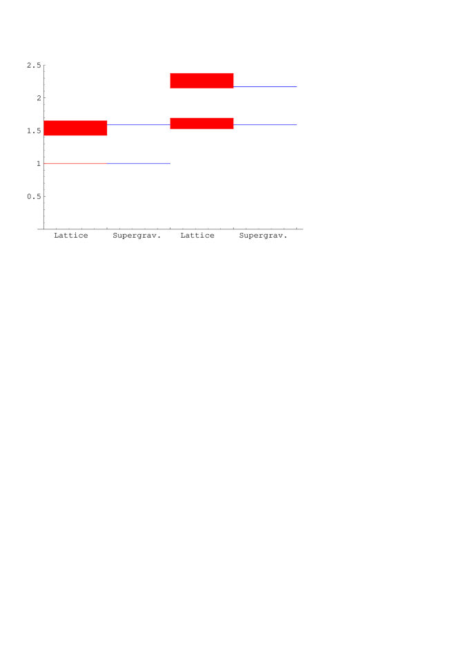
Figure 1: Lattice and supergravity estimates of glueball masses divided by the mass of the $0^{++}$. Shown on the left are the first two $0^{++}$ states; on the right the first two $0^{-+}$ states.

4 Conclusions

I have described how Maldacena’s conjecture can be used to study pure Yang-Mills theories in the large $N$ limit. These methods reproduce several of the qualitative features of QCD, and, in addition, one finds that the supergravity calculations are in a reasonable agreement with the lattice results, even though they are obtained in the opposing limits of the ’t Hooft coupling. It would be very important to understand whether this unexpected agreement is purely a numerical coincidence or whether there is any deeper reason behind it. The historical precedent for a deeper explanation for unexpectedly good results in QCD phenomenology was of course discussed in detail at this conference: some of the successes of the quark model and the Skyrme model are explained in the large $N$ limit!

References

- [1] J. Maldacena, Adv. Theor. Math. Phys. 2, 231 (1998) [Int. J. Theor. Phys. 38, 1113 (1998)] [hep-th/9711200].
- [2] E. Witten, Adv. Theor. Math. Phys. 2, 505 (1998) [hep-th/9803131].
- [3] C. Csáki, H. Ooguri, Y. Oz and J. Terning, JHEP 9901, 017 (1999) [hep-th/9806021].
- [4] S. S. Gubser, I. R. Klebanov and A. M. Polyakov, Phys. Lett. B 428, 105 (1998) [hep-th/9802109]; E. Witten, Adv. Theor. Math. Phys. 2, 253 (1998) [hep-th/9802150].
- [5] M. Teper, [hep-lat/9711011]; see also the talks by M. Teper [hep-ph/0203203] and S. Dalley in these proceedings.
- [6] C. J. Morningstar and M. J. Peardon, Phys. Rev. D 60, 034509 (1999) [hep-lat/9901004].
- [7] R. de Mello Koch, A. Jevicki, M. Mihailescu and J. P. Nunes, Phys. Rev. D 58, 105009 (1998) [hep-th/9806125]; M. Zyskin, Phys. Lett. B 439, 373 (1998) [hep-th/9806128].
- [8] J. A. Minahan, JHEP 9901, 020 (1999) [hep-th/9811156].
- [9] S. S. Gubser, I. R. Klebanov and A. A. Tseytlin, Nucl. Phys. B 534, 202 (1998) [hep-th/9805156].
- [10] H. Ooguri, H. Robins and J. Tannenhauser, Phys. Lett. B 437, 77 (1998) [arXiv:hep-th/9806171].
- [11] J. G. Russo, Nucl. Phys. B 543, 183 (1999) [hep-th/9808117].
- [12] C. Csáki, Y. Oz, J. Russo and J. Terning, Phys. Rev. D 59, 065012 (1999) [hep-th/9810186].
- [13] C. Csáki, J. Russo, K. Sfetsos and J. Terning, Phys. Rev. D 60, 044001 (1999) [hep-th/9902067].
- [14] J. G. Russo and K. Sfetsos, Adv. Theor. Math. Phys. 3, 131 (1999) [hep-th/9901056].
- [15] M. Cvetič and S. Gubser, JHEP 9907, 010 (1999) [hep-th/9903132].
- [16] J. B. Kogut, D. K. Sinclair and L. Susskind, Nucl. Phys. B 114, 199 (1976).