Flux of Atmospheric Neutrinos

Abstract

Atmospheric neutrinos produced by cosmic-ray interactions in the atmosphere are of interest for several reasons. As a beam for studies of neutrino oscillations they cover a range of parameter space hitherto unexplored by accelerator neutrino beams. The atmospheric neutrinos also constitute an important background and calibration beam for neutrino astronomy and for the search for proton decay and other rare processes. Here we review the literature on calculations of atmospheric neutrinos over the full range of energy, but with particular attention to the aspects important for neutrino oscillations. Our goal is to assess how well the properties of atmospheric neutrinos are known at present.

1 Introduction

When primary cosmic-ray protons and nuclei enter the atmosphere their interactions produce secondary, “atmospheric” cosmic rays including all the hadrons and their decay products. The spectrum of these secondaries peaks in the GeV range, but extends to high energy with approximately a power-law spectrum. Because they are weakly interacting, neutrinos were the last component of the secondary cosmic radiation to be studied, and the time-scale for progress has been correspondingly slow. The basic principles of detection and very rough estimates of rates were known by 1960. Markov Markov suggested the idea of detecting neutrino-induced horizontal or upward-moving muons in a detector in a deep body of water and estimated the rates that might be observed MZ . Greisen Greisen estimated roughly the rate of neutrino interactions inside a large, deep Cherenkov detector. Two groups Achar ; Reines independently reported observations of atmospheric neutrinos in 1965 by detecting horizontal muons in detectors so deep that the muons could not have been produced in the atmosphere.

With the advent of very large, deep underground detectors, whose construction was originally motivated by the search for proton decay, there are now extensive measurements of the flux of atmospheric neutrinos in which the events occur within the fiducial volume of the detector. What is emerging from recent studies is a discovery which is likely to have an impact comparable to that of the discoveries made with atmospheric cosmic rays half a century ago, including existence of the pion, the kaon and the muon. The 50 kiloton SuperKamiokande experiment, with a 20 kiloton fiducial volume, has now accumulated sufficient statistics to see clearly that the flux of muon-neutrinos depends not only on the rate at which they are produced in the atmosphere, but also on the pathlength they travel to the detector evidence .

The detector has a cylindrical shape, and its response is up-down symmetric to within a few percent. The atmospheric neutrino beam is also symmetric under reflection about a horizontal plane through the detector–except for geomagnetic effects that we discuss in detail below. There is nevertheless a deficit of upward muon-neutrinos, with pathlengths of order $10^{4}$ km, relative to downward neutrinos, which are produced within tens of kilometers of the detector.

The most likely cause of this pathlength-dependence is neutrino oscillations, in which neutrinos produced as muon-type, after passing a certain distance (which depends on energy), manifest themselves with a different “flavor”, in this case as $\nu_{\tau}$ SuperKtau . The implication of this behaviour is that the neutrinos possess a small but non-zero mass, thus pointing to physics beyond the standard model of particle physics. This discovery has stimulated intense activity to find the implications for particle theory, and to relate this manifestation of neutrino physics to the solar neutrino problem, which is now also understood to be another manifestation of neutrino properties SNO .

The first evidence that atmospheric neutrinos were not behaving as expected came from the observation by IMB that the fraction of neutrino interactions with stopping muons was lower than expected IMB1 . Then Kamioka reported that the ratio of muon-like to electron-like neutrino interactions was lower than expected KAM . The Frejus experiment, however, reported a ratio consistent with expectation  Frejus . These detectors had fiducial volumes ranging from a fraction to a few kilotons. As statistics accumulated from the water detectors (IMB and Kamioka) IMB3a ; IMB3b ; KAM2 ; KAM3 and results were reported from Soudan Soudan , evidence for the atmospheric neutrino anomaly increased. In the last paper from the Kamioka experiment KAMlast , the first evidence for a pathlength dependence characteristic of neutrino oscillations emerged.

In the case of mixing between two flavors of neutrinos, one of which is $\nu_{\mu}$, the probability that a neutrino produced as a $\nu_{\mu}$ travels a distance L and is detected as a $\nu_{\mu}$ is

$$P_{\nu_{\mu}\rightarrow\nu_{\mu}}\;=\;1\,-\,\sin^{2}(2\theta_{m})\,\sin^{2}\left[1.27\,\delta m^{2}{L_{km}\over E_{GeV}}\right],$$ (1)

where $\delta m^{2}=m_{1}^{2}\,-\,m_{2}^{2}$ is the difference of the squared masses of the two related mass eigenstates and $\theta_{m}$ is the angle that characterizes mixing between the two states. Thus the characteristic signature of neutrino oscillations is a deviation from the expected flux as $L/E$ varies. Currently, the best fit to the data of Super-K SuperKtau has $\delta m^{2}\approx 3.2\times 10^{-3}$ eV² with full mixing, $\theta_{m}\approx\pi/4$.

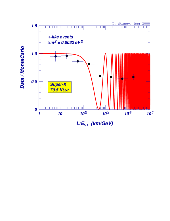
Figure 1: Oscillation probability as a function of $L/E_{\nu}$.

Fig. 1 summarizes the current situation with the measurements of Super-K. One sees that the characteristic first oscillation dip cannot be resolved at present with Super-Kamiokande. This is a consequence of its limited energy and angular resolution coupled with the fact that, with the estimated value of $\delta m^{2}$, the first minimum occurs for pathlengths

$$L\;\approx\;400\,{\rm km}\times E_{\nu}(GeV).$$ (2)

This distance from production in the atmosphere to underground detector corresponds to neutrinos coming from near the horizon where the pathlength changes rapidly with zenith angle. This consideration Lipari1 limits the accuracy with which $\delta m^{2}$ can be determined with the atmospheric neutrino beam. On the other hand Lipari1 the determination of the value of the mixing angle, since it is large, can be very precise with atmospheric neutrinos, limited only by statistics.

Figure 2: Distributions of neutrino energies that give rise to four classes of events. Sub-GeV and multi-GeV refer to the two classes of contained events at Superkamiokande. Stopping and throughgoing muons refer respectively to neutrino-induced muons produced outside the detector.

Contained neutrino events in Super-Kamiokande are classified as sub-GeV and multi-GeV. To probe the atmospheric neutrino spectrum at higher energy it is necessary to make use the older technique of neutrino-induced muons, where the effective volume is the projected area of the detector times the muon range. Since the muon range increases with energy, so does the effective volume. Fig. 2 shows the distribution of neutrino energies for four classes of events. The $\nu_{\mu}\leftrightarrow\nu_{\tau}$ oscillation interpretation that is emerging from the data is also consistent with deviations from the expected angular distributions of neutrino-induced upward muons measured in MACRO MACRO and Super-Kamiokande SuperKupwardthrough and with the ratios of stopping to throughgoing upward muons MACROstopping ; SuperKupwardstopping .

The experimental evidence for oscillations of atmospheric neutrinos is the subject to two recent reviews KT ; Jung . Here we focus on calculations of the atmospheric neutrino flux. In doing so, we will emphasize those aspects that are important for making inferences about oscillations. These include the flavor ratios and angular distributions as well as pathlength distributions as a function of angle.

We will also discuss the absolute normalization of the flux and the energy spectra up to very high energy. While inferences about oscillations emphasize measurements of ratios to minimize their dependence on the absolute accuracy of atmospheric neutrino flux calculations, the normalization is still important for checking the overall consistency of the measurements and calculations. In addition, high energy atmospheric neutrinos constitute the background for neutrino astronomy at all energies. Both Baikal Baikal and AMANDA AMANDA have detected atmospheric neutrinos. Neutrino telescopes with larger effective volume are planned Nestor ; Antares ; Nemo ; IceCube . More important is that the atmospheric neutrinos will be the primary calibration beam for the neutrino telescopes.

We organize the review as follows. After giving an overview of the calculations in §2, in the next three sections we review the primary spectrum, geomagnetic effects and hadronic interactions, which are the principal physical quantities that influence the neutrino spectrum. Then in §6 we turn to a comparison of different calculations. Until recently, nearly all calculations were one-dimensional in the sense that all secondaries were assumed to follow the direction of the parent cosmic-ray from which they descended. In §7 we review the novel features of the recent three-dimensional calculations. Atmospheric muons are closely related to atmospheric neutrinos, and they therefore provide an essential constraint. We review the muon data in relation to the neutrinos in §8. In §9 we enumerate the uncertainties in the various ingredients of the calculations and estimate the resulting uncertainty in the atmospheric neutrino flux.

2 Overview of Neutrino Flux Calculations

The atmospheric neutrino flux is a convolution of the primary spectrum at the top of the atmosphere with the yield ($Y$) of neutrinos per primary particle. To reach the atmosphere and interact, the primary cosmic rays first have to pass through the geomagnetic field. Thus the flux of neutrinos of type $i$ can be represented as

$$\phi_{\nu_{i}}\,=\,\phi_{p}\,\otimes\,R_{p}\,\otimes\,Y_{p\rightarrow\nu_{i}}\,+\;\sum_{A}\left\{\phi_{A}\,\otimes\,R_{A}\,\otimes\,Y_{A\rightarrow\nu_{i}}\right\},$$ (3)

where $\phi_{p(A)}$ is the flux of primary protons (nuclei of mass A) outside the influence of the geomagnetic field and $R_{p(A)}$ represents the filtering effect of the geomagnetic field. Free and bound nucleons are treated separately because propagation through the geomagnetic field depends on magnetic rigidity (total momentum divided by total charge) whereas particle production depends to a good approximation on energy per nucleon. A proton of rigidity $R$ (GV) has total energy per nucleon $E(GeV)=\sqrt{R^{2}+m_{p}^{2}}$ whereas the corresponding relation for helium is $E(GeV/A)=\sqrt{R^{2}/4+m_{p}^{2}}$.

The neutrinos come primarily from the two-body decay modes of pions and kaons and the subsequent muon decays. The decay chain from pions is

$$\pi^{\pm}\rightarrow \mu^{\pm} +\;\nu_{\mu}(\overline{\nu}_{\mu})$$

$$\;\;\;\;\searrow$$

$$e^{\pm}+\nu_{e}(\overline{\nu}_{e})+\overline{\nu}_{\mu}(\nu_{\mu}),$$

with a similar chain for charged kaons. When conditions are such that all particles decay, we therefore expect

$${\nu_{\mu}\,+\,\bar{\nu}_{\mu}\over\nu_{e}\,+\,\bar{\nu}_{e}} \sim 2,$$ (5)

$$\nu_{\mu}/\bar{\nu}_{\mu}\sim 1\; {\rm and} \;\nu_{e}/\overline{\nu}_{e}\sim\mu^{+}/\mu^{-}.$$

Moreover, the kinematics of $\pi$ and $\mu$ decay is such that roughly equal energy is carried on average by each neutrino in the chain.

2.1 Early calculations

The early calculations used the relation between muons and neutrinos implied by Eq. 2. The idea is to parameterize the pion production spectrum in the atmosphere to fit an observed flux of muons. In this way, the primary spectrum and the particle production do not enter the calculation of the neutrino flux explicitly. Since the kinematical relation between neutrinos and their parent pions is different for pions and kaons, some assumption about their relative importance has to be made.

        

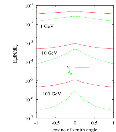
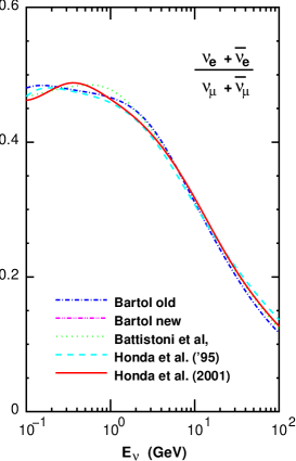
Figure 3: Left panel: Zenith-angle dependence of $\nu+\bar{\nu}$ calculated in the absence of a geomagnetic field. Right panel: Ratio of $(\nu_{e}+\bar{\nu}_{e})/(\nu_{\mu}+\bar{\nu}_{\mu})$ as calculated in several recent papers including the geomagnetic field for the location of Super-Kamiokande (see §6).

Most of the essential features of the atmospheric neutrino spectrum were already displayed and discussed in the 1961 paper of Zatsepin and Kuz’min ZK . Muons with energy of several GeV and above reach the ground before decaying, so the $\nu_{e}/\nu_{\mu}$ ratio decreases with increasing energy. The resulting steepening of the $\nu_{e}$ spectrum occurs at lower energy near the vertical direction and at higher energy near the horizon because of the longer decay path for the parent muons with large zenith angle. The component of the $\nu_{\mu}$ flux from muon decay behaves the same way. For $E_{\nu}>100/\cos\theta$ GeV, the ratio of electron to muon neutrinos approaches a small value $\lower 3.01385pt\hbox{${\buildrel<\over{\sim}}$}5$%, with the main source of $\nu_{e}$ the decay $K_{L}^{0}\rightarrow\pi\,e\,\nu_{e}$. To the extent that there is uncertainty in kaon production, there will be a corresponding uncertainty in this ratio at high energy. These features of the neutrino flux are illustrated in Fig. 3. The left panel shows the neutrino fluxes from Ref. AGLS calculated in the artificial case of no geomagnetic cutoff and shown as a function of cosine of the zenith angle. The right panel shows the key ratio of electron neutrinos to muon neutrinos from several calculations AGLS ; Hamburg ; Battistoni ; Honda ; Hondanew averaged over all directions for the specific location of Super-K.

In calculating neutrinos from decay of muons, it is important to include the effect of muon polarization. Although they did not include it in their calculation, Zatsepin and Kuz’min pointed out that it would have the effect of incrasing the $\nu_{e}/\nu_{\mu}$ ratio by about 5%. Muons are produced fully polarized in the two-body decays of pions and kaons, with the direction of polarization determined by the direction of the muon in the rest frame of its parent. Because of the steep spectrum, the effect does not average to zero in the integral over the parent energies. Moreover, it has the same sign for neutrinos and antineutrinos. Volkova Volkova pointed out the importance of neutrino polarization in the context of the atmospheric neutrino anomaly.

The angular and energy dependence of muons and neutrinos from decay of pions and kaons is determined by the competition between decay and interaction of the parent mesons. The critical energy for pions in the atmosphere is $\epsilon_{\pi}\approx 115$ GeV, and $\epsilon_{K}\approx 850$ GeV for kaons. For $E_{\nu}\ll\epsilon/\cos\theta$ the neutrino spectrum has approximately the same power as the parent meson production spectrum and hence of the primary spectrum of nucleons. For $E_{\nu}\gg\epsilon\cos\theta$ the neutrino spectrum is one power steeper and is proportional to $\sec(\theta)$. Since $\epsilon_{K}>\epsilon_{\pi}$, the spectrum of neutrinos from pion decay steepens before that of neutrinos from decay of kaons, so that kaons become increasingly important at high energy. Since the change of slope depends on zenith angle as well as energy, it is possible in principle to use the observed ($E,\theta$) dependence of the muon flux to estimate, or at least set an upper limit, on the fraction of kaons. Ref. ZK1 used this method to show that atmospheric muons are not dominated by kaons.

The importance of kaons relative to pions is further enhanced at high energies for neutrinos as compared to muons because most of the energy in pion decay goes to the muon as compared to the neutrino, whereas it is divided nearly equally in the $K\rightarrow\mu\nu$ decay. For $E_{\nu}>100$ GeV kaons become the dominant source of neutrinos even though the kaon/pion ratio at production is small.

Perkins Perkins ; Perkins1 has reviewed calculations that reconstruct the neutrino flux from the muon flux. Refinements account for variation of the geomagnetic field over the globe and start from muon data at high altitude where most of the pion and kaon decays occur. Recent calculations, however, use the method of Eq. 3, which is amenable to detailed monte carlo simulations, and we will concentrate on those results in this review.

2.2 Analytic approximations

Before proceeding to the details of the review, it will be helpful to discuss briefly the analytic approximations for the neutrino flux as a guide to the physics of atmospheric neutrinos. Not only do these approximations allow a good qualitative understanding of the features of the atmospheric neutrino flux, but they are valuable for diagnostic purposes, for example, to determine what ranges of primary energy and what regions of phase space in particle production are important for various classes of events. Often, for such diagnostic purposes an approximate representation is adequate.

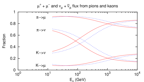
Figure 4: Fractional contribution of pions and kaons to the flux of muons and neutrinos. For pions the bottom curve of each pair is for the vertical and the top curve for zenith angle of $60^{\circ}$. The reverse is true for the kaon fractions.

The analytic approximations apply at high energy ($E_{\nu}\gg 1$ GeV) and hold for a power-law primary spectrum and inclusive cross sections that obey Feynman scaling in the fragmentation region. With these assumptions, the differential flux of $\nu_{\mu}+\bar{\nu}_{\mu}$ from decay of pions and kaons is

$${dN_{\nu}\over dE_{\nu}}\,=\,{\phi_{N}(E_{\nu})\over(1-Z_{NN})(\gamma+1)}\left\{\left[{Z_{N\pi}(1-r_{\pi})^{\gamma}\over 1+B_{\pi\nu}\cos\theta E_{\nu}/\epsilon_{\pi}}\right]+0.635\left[{Z_{NK}(1-r_{K})^{\gamma}\over 1+B_{K\nu}\cos\theta E_{\nu}/\epsilon_{K}}\right]\right\},$$ (6)

where

$$\phi(E_{0})\;=\;{dN\over dE_{0}}\;=\;A\times E_{0}^{-(\gamma+1)}$$ (7)

is the differential primary spectrum of nucleons of energy $E_{0}$. The neutrino flux in Eq. 6 is proportional to the primary spectrum evaluated at the energy of the neutrino. The constants $r_{i}=m_{\mu}^{2}/m_{i}^{2}$ for $i=(\pi,K)$, and the constants $B_{i}$ depend hadron attenuation lengths as well as decay kinematics book . The expression for the flux of $\mu^{+}+\mu^{-}$ has the same form but with different kinematical factors. Similar (somewhat more complex) formulas also exist for neutrinos from decay of muons Paoloanalytic . The approximations become increasingly accurate as energy increases. Eq. 6 displays the features of angular dependence and the relative importance of kaons as described above and illustrated in Fig. 4.

Table 1: Parameters for atmospheric $\nu_{\mu}+\bar{\nu}_{\mu}$ from $\pi$,K-decay

Mass-square ratios	$r_{\pi}$	$r_{K}$	$B_{\pi}$	$B_{K}$
& B-factors:	0.573	.046	2.77	1.18
Characteristic $E_{decay}$:	$\epsilon_{\pi}$	$\epsilon_{K}$	$\epsilon_{charm}$
	115 GeV	850 GeV	$\sim 5\times 10^{7}$ GeV
Z-factors:	$Z_{N}$	$Z_{\pi}$	$Z_{K}$
	0.30	0.079	0.0118

The physics of production of the parent pions and kaons is contained in the spectrum-weighted moments,

$$Z_{N\rightarrow\pi(K)}\;=\;\int_{0}^{1}\,dx\,(x)^{\gamma-1}\,F_{N\rightarrow\pi(K)}(x),\;{\rm etc.},$$ (8)

where

$$F_{N\pi}(E_{\pi},E_{N})\,=\,{E_{\pi}\over\sigma_{N}}\,{d\sigma(E_{\pi},E_{N})\over dE_{\pi}}$$ (9)

is the normalized inclusive cross section for $N\,+\,{\rm air}\rightarrow\pi^{\pm}\,+\,X$. The integrand of the spectrum-weighted moment in Eq. 8 displays the regions of longitudinal phase space in nucleon interactions that are most important for production of neutrinos response .

Table 1 shows a sample set of parameters for the analytic formulas. The same formalism can be used to include neutrinos from decay of charmed particles. These eventually dominate the spectrum at sufficiently high energy because of their short decay length (and correspondingly large critical energy).

2.3 Response functions

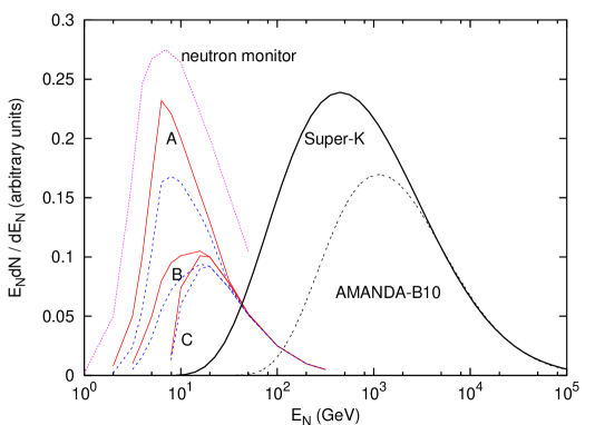
Figure 5: Response to primary energy for several classes of interactions of $\nu_{\mu}+\bar{\nu}_{\mu}$: sub-GeV events (A: no cutoff; B: events from the lower hemisphere; C: events from upper hemisphere at Super-K); vertically upward, throughgoing muons at Super-K and neutrino-induced muons in AMANDA-B10. For the sub-GeV events, each pair of curves shows the range of the signal between minimum (solid) and maximum (dashed) level of solar activity. The dotted curve shows a typical response function for a neutron monitor, to be discussed in §3.3. (The neutron monitor response is plotted vs rigidity rather than energy.)

Response functions give the distributions of primary energy/nucleon that produce neutrinos of a given energy (or distribution of energies). Since the uncertainty in the primary spectrum depends on energy, these functions can be used to evaluate the contribution of this source of uncertainty to the calculated neutrino flux.

For the sub-GeV events the neutrino energies are low enough so that geomagnetic cutoffs and solar modulation become important. These points are illustrated by the curves labelled A, B and C in Fig. 5 and will be discussed further below. Fig. 5 also shows the response for vertically upward throughgoing muons at Super-K and for upward muons in AMANDA B10 as estimated with the approximations of Ref. response . The threshold for the neutrino-induced upward muon at Super-K is $\approx 7$ GeV (vertical) and about an order of magnitude higher for AMANDA B10 AMANDA .

3 Primary Spectrum

Here we describe the primary spectrum inside the heliosphere as it would be measured without the influence of the geomagnetic field. It is important to note that, except for geomagnetic effects, the primary cosmic-ray flux is nearly isotropic. Compton and Getting Compton pointed out that the motion of the earth due to galactic rotation at $\sim 300$ km/s would lead to an asymmetry of order 1% in the relativistic cosmic rays if they there sources were external to the galaxy. Any asymmetry due to the motion of the earth relative to the cosmic-ray gas has come to be known as the Compton-Getting effect. It is now believed that most cosmic rays originate inside the galaxy, so one might expect a smaller anisotropy due to the peculiar motion of the solar system at $\sim 20$ km/s relative to the galactic rotation. Sidereal cosmic-ray anisotropies have been measured to be at the level of $<0.1$% Groom , although a recent analysis Nagashima indicates a more complex origin than the Compton-Getting effect. In any case, such asymmetries are too small to affect the neutrino flux significantly. We discuss the geomagnetic effects, which are important for sub-GeV neutrinos, in the next section.

3.1 Summary of data on protons and helium

In the last decade a series of measurements with superconducting magnetic spectrometers has greatly improved our knowledge of primary cosmic-ray spectra up to 100 GeV/nucleon. At higher energies the situation is not as good. Fig. 6 is a summary of the data for protons and helium. The measurements below 100 GeV are made with balloon-borne magnetic spectrometers Webber ; LEAP ; MASS1 ; MASS ; CAPRICE ; IMAX ; BESS and by the AMS Space Shuttle flight AMS . Measurements at higher energy have been made by balloon-borne calorimeters of various kinds Ryan ; JACEE ; Ivanenko ; Runjob ; Kawamura . These do not capture all the energy of the primary, and as a consequence, the energy determination is not as precise as with a spectrometer.

Starting with the LEAP experiment LEAP , the measured fluxes have been consistently lower that of Ref. Webber , which had previously been the standard. Particularly remarkable is the close agreement between the BESS BESS and AMS AMS measurements of the proton flux. They agree with each other to better than 5% over their whole energy range. In contrast there is a systematic difference of about 15% between the BESS and AMS measurements of helium. Note, however, that only some 25 % of all nucleons is carried by helium and heavier nuclei, so such a difference corresponds to an uncertainty of $\sim$ 3 % in the flux of nucleons.

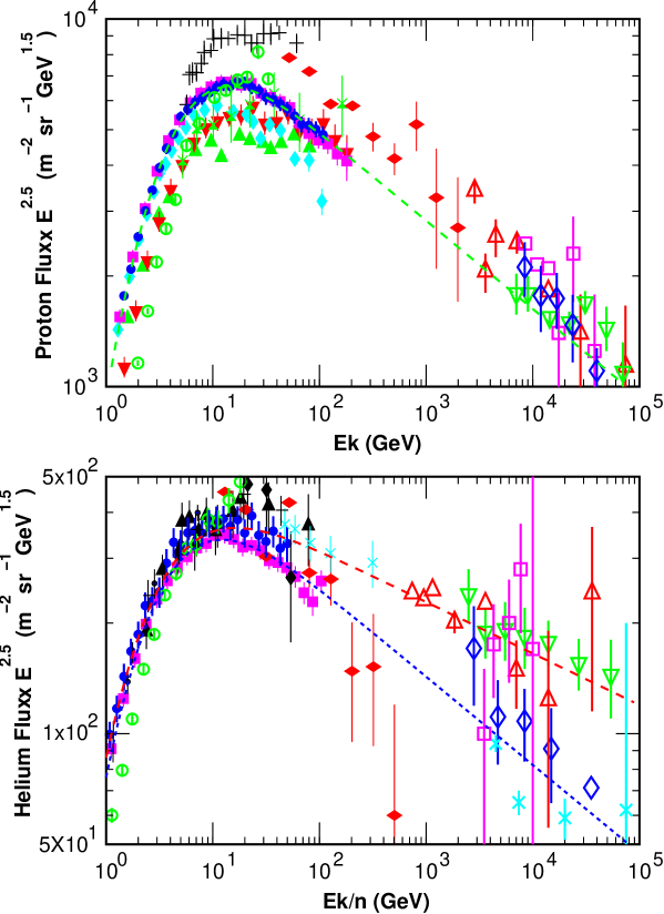
Figure 6: Observed flux of cosmic-ray protons and helium. The dashed lines show the fits described in the text. The data are: Webber Webber -crosses; LEAP LEAP -upward triangles; MASS1 MASS1 -open circles; CAPRICE CAPRICE -vertical diamonds; IMAX IMAX -downward triangles; BESS98 BESS -circles; AMS AMS -squares; Ryan Ryan -horizontal diamonds; JACEE JACEE -downward open triangles; Ivanenko Ivanenko -upward open triangles; Kawamura Kawamura -open squares; Runjob Runjob -open diamonds.

Ref. spectrum discusses the measurements of the primary spectrum in the context of atmospheric neutrinos. Fits of the form

$$\phi(E_{k})\;=\;K\times\left(E_{k}\,+b\,\exp\left[-c\sqrt{E_{k}}\right]\right)^{-\alpha}$$ (10)

are given, with parameters as tabulated in Table 2. The fits for protons and helium are determined largely by the AMS AMS and BESS BESS data, with their small statistical uncertainties. They are shown as dashed lines in Fig. 6. Parameters for the three groups of heavy nuclei in Table 2 have been updated by Stanev Stanev-private since publication of Ref. spectrum .

Table 2: Parameters for all five components in the fit of Eq. 10.

parameter/component	$\alpha$	K	b	c
Hydrogen (A=1)	2.74$\pm$0.01	14900$\pm$600	2.15	0.21
He (A=4, high)	2.64$\pm$0.01	600$\pm$30	1.25	0.14
He (A=4, low)	2.74$\pm$0.03	750$\pm$100	1.50	0.30
CNO (A=14)	2.60$\pm$0.07	33.2$\pm$5	0.97	0.01
Mg-Si (A=25)	2.79$\pm$0.08	34.2$\pm$6	2.14	0.01
Iron (A=56)	2.68$\pm$0.01	4.45$\pm$0.50	3.07	0.41

3.2 Heavier nuclei and the all-nucleon spectrum

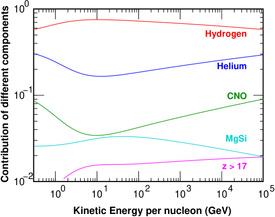
Figure 7: Fractional contributions of various nuclei to the all-nucleon spectrum spectrum .

Production of pions and kaons in the atmosphere, and hence, the neutrino flux, depends essentially on the spectrum of nucleons as a function of energy-per-nucleon. Protons and neutrons must be treated separately to obtain the charge ratio and the correct $\bar{\nu}/\nu$ ratios. Bound and free protons must be passed separately through the geomagnetic filter since the relation between energy per nucleon and rigidity is different for free protons and for nuclei.

A fit for the all-nucleon spectrum outside the magnetosphere corresponding to Eq. 10 can be constructed directly from Table 2. Fig. 7 shows the fractional contributions of protons, helium and three groups of heavy nuclei. In the energy range important for the contained neutrino interactions, protons contribute 75%, helium 15% and all heavier nuclei about 10%.

3.3 Solar modulation

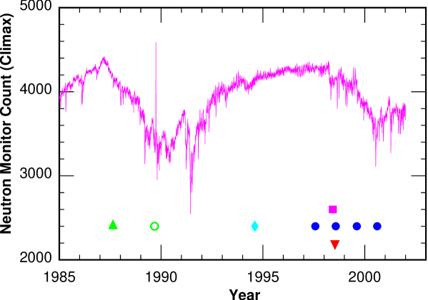
Figure 8: Record of count rates for the Climax neutron monitor Climax . Times of the various flights are marked using the same symbols as in Fig. 6.

The sun emits a magnetized plasma with a velocity of $\approx 400$ km/s in the solar equatorial region and about twice as high over the solar poles Ulysses . To reach the earth and interact in the atmosphere, galactic cosmic rays have to diffuse into the inner heliosphere against the outward flow of the turbulent solar wind, a process know as solar modulation. Particles of very low energy outside the heliosphere are nearly completely excluded, while higher energy particles lose energy as they diffuse in. During periods of high solar activity (“solar maximum”) the turbulence in the solar wind is higher than during solar minimum and the low-energy portion of the spectrum is more suppressed.

A classic tool for study of solar modulation is the neutron monitor Simpson . Response functions for neutron monitors Clem are similar to the response for sub-GeV neutrinos, as illustrated by the dotted curve in Fig. 5. As a consequence, neutron monitor records Bartol ; Climax provide an ideal tool for interpolating between the spectra measured at particular instants of the solar cycle. Fig. 8 is a plot of the Climax neutron monitor Climax with the dates of the flights on which the low-energy data in Fig. 6 were obtained. Except for MASS1 MASS1 , most of the flights were close to solar minimum conditions, and the shapes of their low-energy spectra are similar. The MASS1 data, which were obtained in 1989 during solar maximum conditions, show extra suppression at low energy.

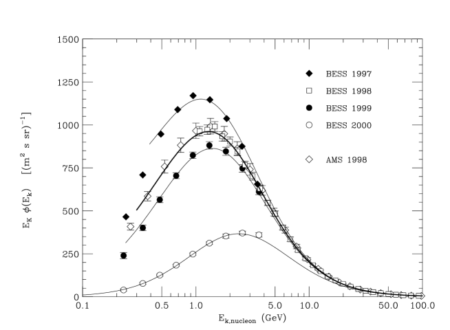
Figure 9: Proton spectra measured by BESS in 1997, 1998, 1999 and 2000 Asaoka . Curves are explained in the text.

It is possible to use the neutron monitor count rate ($N_{m}$) as a parameter to relate the spectrum at one phase of the solar cycle to that at another. The parameterization of Ref. Nagashimaetal was used in Ref. Honda to provide a multiplicative factor by which a time-independent reference spectrum is multiplied. The factor is a function both of particle momentum and $N_{m}$. Recently a new set of data taken with the BESS detector at three different levels of solar activity (including one in 2000 during solar maximum) has been published Asaoka . We show these data, together with the BESS98 data from Fig. 6, in Fig. 9. The curves in Fig. 9 are obtained by Lipari Paolo-private starting with Eq. 10 for the 1998 BESS data and using the force-field approximation forcefield . In this simple approximation the phase space density of particles is shifted down in energy by an amount $\Delta\Phi$ that depends only on $N_{m}$ and not on momentum. When the BESS-2000 data for $E>4$ GeV becomes available it will be possible to refine the way the spectrum modulates as a function of energy. At the same time, the data should provide the basis for an improved understanding of solar modulation. In the meantime, we can estimate roughly (see Fig. 5) that solar modulation should be a 10% effect at Kamioka and a 20% effect at the high latitude sites, Soudan and Sudbury.

4 Geomagnetic effects

The geomagnetic field affects cosmic rays both outside and inside the atmosphere. Outside it acts as a filter which allows in particles of sufficiently high energy and excludes those of lower energy. Inside it bends charged secondaries causing some important effects which we discuss later. Whether a particle is allowed or forbidden is determined by its position, direction, and radius of curvature. Only those particles that interact in the atmosphere before curving back into space can contribute to the flux of atmospheric neutrinos. Because the effect depends on the gyroradius of a particle, the relevant kinematic variable is total momentum divided by total charge, i.e. rigidity.

In case of a dipole magnetic field centered on the earth, the cutoff rigidity can be expressed in an analytic form by Störmer’s formula Stormer ; Alpher :

$$R_{S}^{\pm}(r,\lambda_{M},\theta,\varphi)=\left({M\over r^{2}}\right)~{}\left\{{\cos^{4}\lambda_{M}\over[1+(1\lower 3.01385pt\hbox{${\buildrel-\over{+}}$}\cos^{3}\lambda_{M}\sin\theta\sin\varphi)^{1/2}]^{2}}\right\},$$ (11)

where $r$ is the distance from the center of the earth and $\lambda_{M}$ is the geomagnetic latitude, $\theta$ and $\varphi$ define the arrival direction of the cosmic ray, and $M=8.1\times 10^{25}$ G cm³ is the magnetic dipole moment of the earth. The azimuthal angle of the direction vector of the particle is $\varphi$, measured counterclockwise from magnetic north. Thus a particle arriving from the west has $\sin\varphi<0$ giving a lower cutoff for a positive particle (upper sign in Eq. 11). A positive particle arriving from the east has a higher cutoff. The scale is set by the maximum cutoff $eM/r_{\oplus}^{2}=60$ GeV, which is the energy at which a proton approaching from the east at the equator will orbit the earth.

4.1 Cutoffs for realistic magnetic field

The actual magnetic field is more complicated than a symmetric dipole, and such a simple expression as Eq. 11 is not available. The geomagnetic field is generally expressed as a multipole expansion, and its global structure is well known geomagfield .

The cutoff rigidity for a realistic geomagnetic field can be calculated by the back tracing technique. An anti-proton, which has the same mass as a proton but the opposite charge, is used as the test particle. We note that the change $e\leftrightarrow-e$ is equivalent to the change of $t\leftrightarrow-t$ in the equation of motion of a charged particle in a magnetic field. We launch anti-protons from the top of the atmosphere of the Earth, varying the position and direction to obtain the coverage needed for a given detector location. Standard practice is to define the escape sphere at 10 earth radii. The rigidity cutoff is calculated as the minimum momentum with which the test particle escapes from the geomagnetic field. For some directions at some locations the situation is still more complicated. There can in some cases also be forbidden trajectories in a narrow region just above the minimum cutoff LScut .

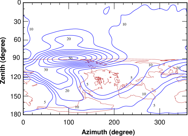
Figure 10: Contour map of the rigidity cutoff as seen from the Kamioka site, Rigidity cutoffs are shown as a function of arrival direction of the neutrino. (Zenith angle $>90^{\circ}$ is for upward-moving particles.) An outline map of the continents is superimposed on the lower hemisphere.

The back tracing technique only tells us if there is a path along which a cosmic ray of a particular momentum and charge can reach the top of the atmosphere. To know the spectrum at the top of the atmosphere, however, one also needs Liouville’s theorem, which ensures the conservation of particles in phase space. Then, assuming that the distribution of cosmic rays outside the heliosphere is isotropic and assuming no change in magnitude of momentum along the path, the flux of particles at the atmosphere has the same value as in interstellar space for allowed values of momentum.

     

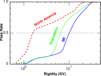
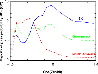
Figure 11: Cutoffs at three locations: north-central North America (Soudan, Sudbury); Gran Sasso; Kamioka. The left panel shows the passing rate as a function of rigidity integrated over all directions. The right panel shows the rigidity above which half the particles in the azimuthal band at each zenith angle reach the atmosphere. (Positive $\cos\theta$ refers to downward-moving particles.)

For a one-dimensional calculation, one can make a contour map of the cutoffs for each detector as a function of direction along the line of sight from the detector. Each entry is the cutoff in the atmosphere where the neutrino trajectory originates. Such a contour map for the cutoffs at Kamioka is shown in Fig. 10 Honda . In the case of a three dimensional calculation, the treatment of geomagnetic cutoffs is very considerably more complex. Since the direction of the neutrino can be at an angle relative to the primary cosmic ray that produced it, one needs the cutoffs for all directions at every point around the globe.

The qualitative effects of the geomagnetic cutoffs at different locations on the globe can be displayed by comparing averaged cutoffs. The left panel of Fig. 11 plots the fraction of $4\pi$ sr allowed as a function of rigidity. The second panel shows the cutoffs averaged over azimuth plotted as a function of zenith angle. (The average cutoff for a given zenith is defined as the rigidity at which 50% of the directions in the azimuth band are allowed.) The three locations are North America (Sudbury and Soudan), Gran Sasso and Kamioka in increasing order of average cutoff. While the average cutoffs for the lower hemisphere ($\cos\theta<-0.5$) are similar for all locations (because they involve averaging over large portions of the surface of the earth) the local cutoffs are quite different. In particular, the up-down ratio at Super-K is opposite to that at the high-latitude sites in North America. Moreover, the geomagnetic up-down ratio at Super-K is such as to suppress downward events, which is opposite to the observed pathlength dependence.

4.2 East-West Effect

Kamioka is at a rather low geomagnetic latitude and has therefore a rather high local cutoff, $\approx 11$ GV. In addition, there is a strong azimuthal asymmetry, with the cutoff higher for particles arriving from the east than from the west. The east-west asymmetry follows from the fact that the primary cosmic rays are positively charged. Historically, it was the east-west asymmetry that led to the conclusion that the primary cosmic rays are positively charged Johnson ; Alvarez . A remarkable feature of the Super-K is that it has been possible to measure SuperKEW the classic east-west asymmetry of the primary cosmic rays as reflected in neutrinos LSG ; Honda . Quantitative understanding of this feature of the data confirms that deviations of the atmospheric neutrino beam from isotropy can be understood entirely as arising from effects of the geomagnetic field.

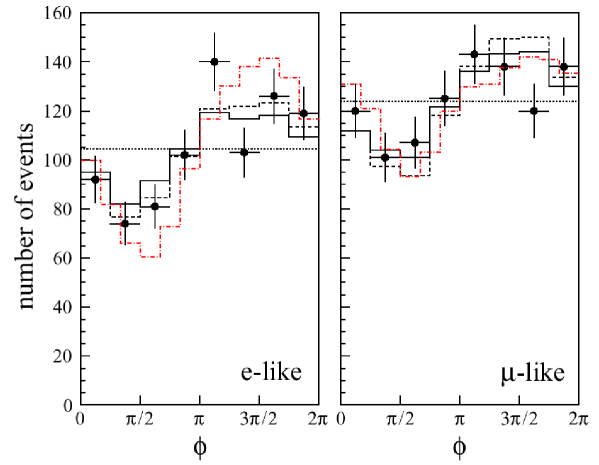
Figure 12: East West effect observed by neutrino. Data points are from SK experiment, and solid and dashed lines are prediction by using the one-dimensional calculation of Honda et al. and Bartol group. Dash-dot are predictions by Lipari taking into account the muon bending normalized by the average value.

In the Fig. 12, we show the experimental data with the predictions. It is seen that the experimental data agree with the predictions well within the experimental errors. However, Lipari pointed out that the azimuthal variation of $\nu_{e}$ events is somewhat larger than the predictions of the one-dimensional calculations, while the azimuthal variation of the $\nu_{\mu}$ events is smaller Lipari-ew . He argues that these details are a consequence of bending of muons by the geomagnetic field inside the atmosphere, which is neglected in the one-dimensional calculations.

Roughly speaking, the $\mu^{+}$ bending enhances the E-W effect for the primary cosmic rays, since the $\mu^{+}$ has the same charge as primary cosmic rays. On the other hand the $\mu^{-}$ bending works to cancel the E-W effects. Therefore the azimuthal variation of $\nu_{e}$ and $\bar{\nu}_{\mu}$ is enhanced by the muon bending above the prediction of the one-dimensional calculations. On the other hand, the azimuthal variation of $\bar{\nu}_{e}$ and $\nu_{\mu}$ are reduced. Considering the fact that the interaction cross sections for $\nu$’s are $\sim$ 3 times larger than $\bar{\nu}$’s at $\sim$ 1 GeV, the muon bending enhances the variation of electron events in the detector and reduces the variation of muon events.

In Fig. 12 the data are plotted as a function of azimuth for a fixed band of zenith angles. Thus any pathlength-dependence affects all events in the band in the same way. The fact that the observed azimuthal variation can be understood entirely as a consequence of geomagnetic effects therefore confirms that the observed pathlength dependence (i.e. dependence on zenith angle) is not due to a poorly understood geomagnetic effect, but is a consequence of pathlength- dependence of the neutrinos.

4.3 Second (subcutoff) spectrum

The AMS detector on the Space Shuttle found and measured AMS2 at 380 km altitude a population of partially trapped particles below the local geomagnetic cutoff. This population is related to the cosmic-ray albedo previously known from stratospheric balloon flights above 30 kilometers (see, for example, albedo ; albedo2 ). It originates when higher energy cosmic rays above the local geomagnetic cutoff interact in the atmosphere and produce secondaries that curve away from the earth. Some of the secondaries may be below the local geomagnetic cutoff, in which case they eventually re-enter the atmosphere as re-entrant albedo reentrant .

Figure 13: Proton spectrum measured AMS2 at various geomagnetic latitudes by the AMS detector on Space Shuttle compared to calculations of Ref. Zuccon . The figure is from Ref. Zuccon .

Several authors Derome ; Lipari2 ; Zuccon have analyzed this “second spectrum” recently by performing 3-dimensional calculations which reproduce the data and allow them to make conclusions about its origin and properties. Since only a small fraction of the secondary nucleons move away from Earth, the intensity of the sub-cutoff population is significantly lower than would be the case in the absence of a geomagnetic field. In addition, a fraction of the particles in the equatorial region remains trapped for several cycles, so that the rate at which these particles re-enter the atmosphere is lower (by a factor equal to the inverse of the number of trapped cycles) than what is measured at 380 km. The reduction of the re-entrant flux is greatest in the equatorial region where the cutoff is generally high. On average, the re-entrant sub-cutoff flux above the threshold for significant pion production is always at least an order of magnitude below the flux at the cutoff energy Zuccon . All these points are nicely illustrated in the figure from Ref. Zuccon that compares AMS data AMS2 with their calculations. The panels in Fig. 13 show a succession of bins of geomagnetic latitude from the equator ($\Theta_{M}=0$) to the poles ($\Theta_{M}=\pm 1$). The dashed line shows the reduced rate at which the sub-cutoff particles re-enter the atmosphere and so become available for neutrino production. In addition, the neutrino yield per incident particle is lower below the cutoff than above. As a consequence, the contribution of the sub-cutoff particles to the neutrino flux is small, though it remains to be calculated precisely.

It is interesting to note that the contribution of the subcutoff particles to the neutrino flux is included in the one-dimensional calculation since all secondary nucleons are assumed to go forward.

5 Hadronic interactions

The third factor in Eq. 3 is the yield of neutrinos per incident cosmic-ray nucleon. For fixed $E_{\nu}$ the yields grow strongly with increasing primary energy. At the same time, the primary spectrum falls quickly as energy increases, to give distributions like those shown in Fig. 5.

Yields are calculated for events generated from primary cosmic rays of various energies and mass, and the events are then weighted according to an appropriate energy spectrum and mass composition. Several technical details of the cascade calculations, in particular muon energy loss and decay, require care in their implementation. The only fundamental source of uncertainty in the yields, however, is from the treatment of particle production in the individual collisions that make up the atmospheric cascades.

Two independent flux calculations AGLS ; Honda have been widely used for interpretation of measurements of atmospheric neutrinos. Both are one-dimensional. More recently, new, three-dimensional calculations have been made Battistoni ; Lipari3D ; Hondanew , which remove the major technical approximation of the original calculations. Differences among the calculations are at the level of 20% in overall magnitude and 5% or less in the ratios $\nu_{e}/\nu_{\mu}$ and $\bar{\nu}/\nu$. Although there are significant differences between the 3D and 1D calculations Battistoni ; Lipari3D ; Hondanew , especially in the angular distributions of sub-GeV neutrinos near the horizon, the major differences are due rather to differences in the treatment of pion production and in the primary spectrum.

5.1 Cross sections

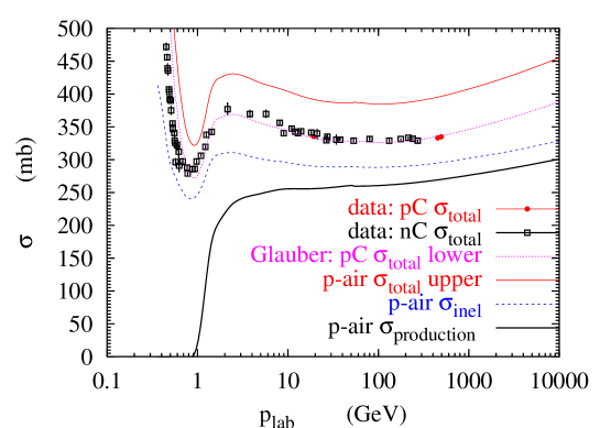
Figure 14: Plot of the total, inelastic and production p-air cross sections. Also shown is a comparison of the p-carbon total cross section with accelerator data. The step in the p-air production cross section at 1 GeV/c corresponds to the onset of significant pion production.

The starting point for calculation of the atmospheric cascade is a set of energy-dependent interaction lengths for the various particles in the cascade. In the approximation that the target in each interaction is treated as an average “air” nucleus, $\lambda_{i}({\rm g/cm}^{2})\,\approx\,14.5m_{p}/\sigma$. It is straightforward to treat the components separately with partial interaction lengths for 78% nitrogen, 21% oxygen and 1% argon by volume. If (as in Ref. AGLS ) quasi-elastic interactions in which the target nucleus fragments without pion production are not included when nucleons interact in the atmosphere, then the corresponding partial inelastic cross section in which at least one secondary meson is produced is used to obtain the interaction lengths. If quasi-elastic processes are included in the event generator (as in Ref. FLUKA ) then the total inelastic cross sections are used to obtain the interaction lengths. Fig. 14 shows a plot of the nucleon-air cross sections ($\sigma_{tot}$, $\sigma_{prod}$ and $\sigma_{inel}$). The quasi-elastic cross section is $\sigma_{QE}\;=\;\sigma_{inel}\,-\,\sigma_{prod}$.

The p-air cross sections have been calculated Private from the parameters of the measured proton-proton cross section (elastic and total cross section, slope parameter and ratio of real to imaginary part of the forward scattering amplitude) using the Glauber multiple scattering formalism GM . To illustrate how well the formalism works, Fig. 14 also shows the total cross section for carbon calculated in the same way compared with an extensive collection of data Dersch . For lab energies corresponding to $\sqrt{s}>2$ TeV, where there are not yet any direct measurements of the proton-proton cross sections, the proton-air cross section becomes somewhat uncertain. Since $\sqrt{s}=2$ TeV is equivalent to a lab energy of $\approx 2$ PeV, this is not an important source of uncertainty even for the neutrino-induced muons.

Concerning treatment of incident nuclei, there are two aspects to consider. First, one needs a set of cross sections and interaction lengths for the various nuclei. In addition, an algorithm for production of secondary particles is needed. The usual approach is to neglect possible coherent effects and use the Glauber multiple scattering theory to determine a number of nucleon-nucleon interactions in each encounter. This can be done with a monte carlo realization of the multiple scattering calculation to determine the number of interacting pairs event-by-event. Then the model for pion and kaon production in nucleon-nucleon collisions is invoked. A further approximation sometimes used is to determine the number of wounded nucleons in the projectile and then immediately use the model for particle production in nucleon-air collisions. In this approximation JEngel , incident nuclei of mass A and energy $E$ are equivalent to A nucleons each of energy per nucleon $E/A$.

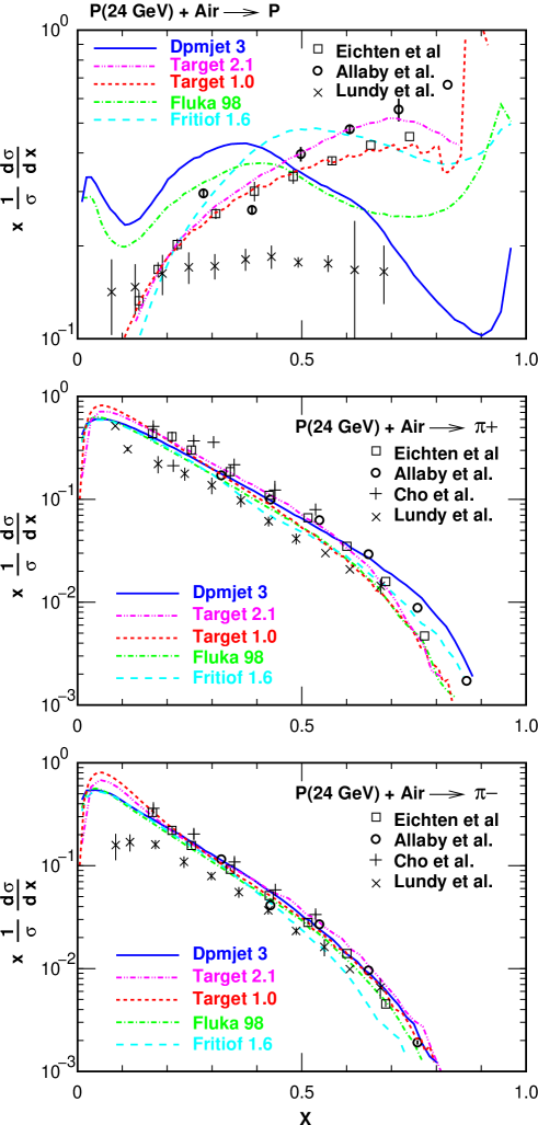
Figure 15: Inclusive cross sections for protons (top); $\pi^{+}$ and $\pi^{-}$ (bottom).

5.2 Pion and kaon production by protons

The models of hadroproduction in use for calculations of the atmospheric neutrino flux are based in one way or another on accelerator data for protons on light nuclei. Most such experiments were done as studies for design of accelerator neutrino beams. A good example is the work of Cho et al. using 12.4 GeV/c beams at the Argonne ZGS on a beryllium target Cho . They measured $d\sigma/dpd\Omega$ as a function of secondary particle momentum with the spectrometer at several angles. They then used a standard four-parameter fit to the double differential cross section SW to find smooth fits to the data. Similar experiments in the region around 20 GeV/c were made at the CERN PS Allaby ; Eichten and at 15 GeV/c at BNL Abbott . Figs. 15 shows the data from these and other Lundy experiments as inclusive distributions integrated over angle using the same parameterization SW to interpolate and extrapolate into unmeasured regions of phase space. The integration requires an extrapolation into unmeasured regions of transverse phase space, which leads to uncertainties in addition to those associated with the measurements, as discussed in Ref. Engel .

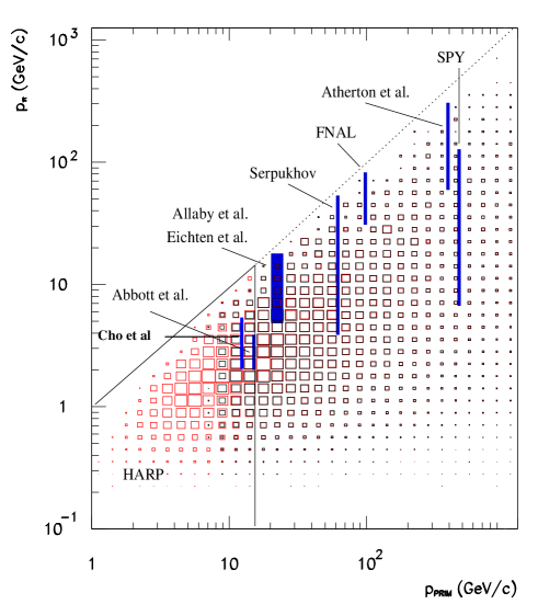
Figure 16: Weighted phase space distribution for sub-GeV atmospheric neutrinos.

The coverage of phase space in the accelerator measurements is generally not matched ideally to the atmospheric neutrino problem. Fig. 16 shows the regions of phase space for proton-air interactions that contribute to the sub-GeV neutrino signal at Super-K, as calculated with the FLUKA program FLUKA ; BatPrivate . The important region shifts to the right for higher energy neutrinos in a way that can be estimated from the response functions discussed above (see Fig. 5). Superimposed on the figure are the regions of phase space covered by the main data sets used for tuning models of hadroproduction for calculation of atmospheric neutrinos. One can note in particular that the region for $p_{beam}\geq 20$ GeV/c and $p_{\pi}<4$ GeV that is important for the sub-GeV events is not covered.

The curves in Fig. 15 show some of the inclusive cross sections in use for calculations of atmospheric neutrinos. Dpmjet3 Dpmjet3 is the event generator currently used by Honda et al. Hondanew , who previously Honda used Fritiof 1.6 Fritiof1-6 . Target 1.0 is the event generator of the Bartol group AGLS , and Target 2.1 is a preliminary revised version Hamburg . The calculation of Battistoni et al. Battistoni uses the interaction model embedded in the FLUKA FLUKA cascade program.

The differences shown here are one of two main components responsible for the differences at the level of 15% among the calculations of Refs. AGLS ; Honda ; Battistoni and Hondanew ; Hamburg . The other main factor is the treatment of the primary spectrum. We comment further on these differences in the next section.

     

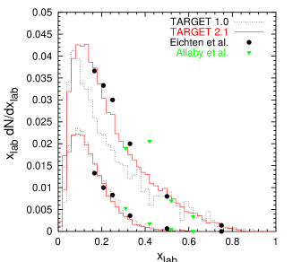
Figure 17: Left panel: Integrated inclusive cross sections for kaon production from Ref. Engel . The upper set of points and histograms is for $K^{+}$, while the lower is for $K^{-}$. Right panel: Multiplicity of $\Lambda$ and $\bar{\Lambda}$ production in proton-proton interactions from Refs. Lam

The process $p\rightarrow\Lambda K^{+}$ makes an important contribution to production of strangeness, and it accounts for the large excess of $K^{+}$ over $K^{-}$ in the fragmentation region. The effect is clearly visible in Fig. 17a, and it becomes increasingly important at high energy as kaons begin to dominate the neutrino flux (see Fig. 4.) Fig. 17b summarizes data on production of $\Lambda$ and $\bar{\Lambda}$ in pp collisions. The difference ($\Lambda\,-\,\bar{\Lambda}$) corresponds to $p\rightarrow\Lambda K^{+}$. Because of the steep primary spectrum, this process is weighted heavily in the spectrum-weighted moments for kaons that enter into the calculated fluxes of neutrinos.

5.3 High energies

At sufficiently high energy the most important contribution to the neutrino flux will come from decay of charmed hadrons, the “prompt” flux, so called because of the short lifetimes of charmed particles. The critical energy for charm decay is $\sim 5\times 10^{7}$ GeV. Thus the neutrinos from decay of charmed hadrons continue with the same spectral index as the primary cosmic-ray spectrum up to this energy, while the neutrinos from decay of pions and kaons become steeper at much lower energy. Moreover, the prompt contribution is isotropic up to $\sim 10^{7}$ GeV while the contribution from pions and kaons is proportional to $\sec(\theta)$ for $E_{\nu}\gg 1$ TeV. As a consequence, even though $Z_{\rm charm}\ll Z_{\pi,K}$, the contribution from charm decay dominates the neutrino spectrum at sufficiently high energy.

Predictions in the literature for the crossover energy differ by several orders of magnitude. Costa Costa surveys a wide range of calculations of prompt leptons. An analysis of the angular dependence of measurements of high-energy atmospheric muons (fitting to an isotropic plus a secant $\theta$ term) VolkovaC suggests that the crossover energy may be as low as $\sim 10$ TeV. At the other extreme, in a perturbative QCD calculation, Thunman et al. Gondolo showed the crossover only around $E_{\nu}\sim 1000$ TeV. A more recent improved QCD calculation Reno puts the crossover around $~{}100$ TeV.

A concern with the perturbative QCD approach in the context of prompt cosmic-ray leptons is that it does not explicitly include the charm analog of $p\rightarrow\Lambda K^{+}$ discussed above. The $\Lambda$ multiplicity plot in Fig. 17b allows an estimate of the probability per interaction of producing a forward $\Lambda K^{+}$ pair as $\approx 0.04$ (by subtracting $\bar{\Lambda}$ from $\Lambda$ and dividing by 2 to get the forward-moving particles). If we assume the production of massive hadrons with similar quark content is inversely proportional to the square of the masses GH , then we can estimate the probability of the corresponding charmed process $p\rightarrow\Lambda_{C}D^{0}$ as

$$P_{\rm forward\;charm}\;\sim\;0.04\times\left(M_{\Lambda}+M_{K}\over M_{\Lambda_{C}}+M_{D}\right)^{2}\;\sim\;0.006.$$ (12)

The actual calculation of the prompt lepton spectrum requires an assumption about the shapes of the inclusive cross section for production of the various charmed hadrons as well as accounting for the various relevant branching ratios and decay distributions. Bugaev et al. Bugaev have systematically calculated prompt muon production in a recombination quark-parton model, which explicitly includes the important fragmentation process.

6 Comparison of neutrino flux calculations

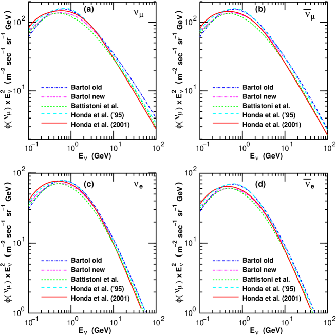
Figure 18: Comparison of neutrino flux calculations for the location of Kamioka averaged over all directions.

Comparing independent calculations is one way to assess the uncertainty in our knowledge of the atmospheric neutrino flux. Fig. 18 is a plot of the flux at Kamioka as calculated by three groups. The calculations of the Bartol group AGLS and Honda et al. Honda , both one-dimensional, are quite similar between 300 MeV and 10 GeV, but the similarity results to some extent from compensating differences in input. The primary spectrum normalization is higher in Ref. Honda than in Ref. AGLS while the pion production is lower. In contrast, the three-dimensional calculation of Battistoni et al. Battistoni uses exactly the same primary spectrum as Ref. AGLS and finds a neutrino flux some 15% lower in the same energy region. As mentioned above, this difference is primarily a consequence of differences in pion production and not a consequence of the 3-dimensional nature of the calculation. The new one-dimensional calculation of Honda et al. uses a new model for pion production and a new and lower primary spectrum.

The interaction models used by these three groups represent three different approaches to the problem. Target is a simple phenomenological representation of pion and kaon production in interactions of protons, pions and kaons with light nuclei Hamburg . Energy conservation is used as an important constraint in adjusting fits to the data. When events are generated, the fragment nucleon from the projectile is selected first, and the remaining energy distributed among pions. As a consequence, the fit to the fast nucleons is of primary importance. Honda et al. use more sophisticated event generators designed for monte carlo studies at accelerators, Fritiof 1.6 in Ref. Honda and Dpmjet3 more recently Hondanew . FLUKA FLUKA is a cascade code that includes generation and propagation of secondary particles of all types in hadronic interactions of all types as an integral part of a cascade code adaptable for any purpose.

 

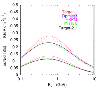
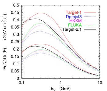
Figure 19: Angle-integrated neutrino fluxes ($\nu+\bar{\nu}/3$) at Kamioka (left) and Soudan (right) with several different interaction models: HKKM Honda , Dpmjet3 Hondanew , FLUKA Battistoni , Target 1.0 AGLS and Target 2.1 Hamburg . The upper set of curves is for muon neutrinos and the lower set for electron neutrinos.

To focus on differences caused by the treatment of hadronic interactions, we refer to Fig. 19. Exactly the same primary spectrum and composition (that from Ref. AGLS ) have been used by Battistoni et al. Battistoni and by the Bartol group AGLS ; Hamburg . Although different primary spectra have been used in Refs. Honda ; Hondanew , the results shown here are from special calculations with the hadronic interaction models used in the published paper but using a primary spectrum identical to that of Ref. AGLS . Therefore, the only differences among these results are due to the differences in treatment of hadronic interactions. It should be possible to trace the differences in the neutrino fluxes shown here back to differences in interaction models such as those shown in Fig. 15. For example, the excess of pions in $\sim 20$ GeV interactions in Target 1.0 as compared to Target 2.1 and FLUKA corresponds to the larger calculated flux at Kamioka. The larger difference among the three calculations at Soudan points to differences in treatment of low-energy interactions that are important at Soudan but not at Kamioka with its higher cutoff.

In the past two years several new calculations of the flux of atmospheric neutrinos have appeared. They are summarized in Table 3 with a comment indicating their normalization relative to Ref. Battistoni . Some of the recent calculations show rather large differences from those discussed so far. The comparisons discussed above, however, suggest that uncertainties in normalization due to hadronic interactions are $<\pm 15$% (and somewhat larger at higher energy where the kaon contribution is more important). Differences in ratios such as $\nu_{e}/\nu_{\mu}$ are significantly smaller, at the level of $5$% (see Fig. 3). Combining a $\pm 15$% estimate of uncertainty from hadronic interactions in quadrature with an estimate of $\pm 20$% for the primary spectrum gives an estimated uncertainty of $\pm 25$%. Even if the estimates are simply added algebraically, it seems difficult to account for differences of a factor of two within the uncertainties in the input.

Table 3: Calculations of the atmospheric neutrino flux

Reference		Comment
FLUKA0Battistoni	3D	1
New Bartol0Hamburg	1D	$\approx 1$ (preliminary)
Honda et al.0Hondanew	3D	$+10$ to $15$%
SNO sub-group0Tserk	3D	$\sim 1$
Fiorentini et al.0Fior	1D	$-20$% for sub-GeV; $\sim 1$ for $>$GeV
CORSIKA0Wentz	3D	$\sim 1$ (preliminary)
Grenoble0Liu	3D	$\sim{1/2}$
Plyaskin0Plyaskin	3D	$<{1/2}$

7 Three-dimensional calculations

The major technical limitation of most calculations of the atmospheric neutrino flux until recently is that they are one-dimensional; in other words, it is assumed that all secondaries move in the direction of the primary particle from which they descend. This approximation neglects the transverse momentum of the secondaries as well as their bending in the geomagnetic field as they propagate. The latter is most important for muons and their decay products because of the muon’s long decay length. A muon with Lorentz factor $\gamma$ typically bends by an angle

$$\theta\;\sim\;\gamma\,c\,\tau_{\mu}\,/\,r_{L},$$ (13)

where $r_{L}\,\approx\,E_{\mu}\,/\,eB$ is its gyroradius in the geomagnetic field. Dependence on $E_{\mu}$ cancels in Eq. 13, and typical bending is $\sim 3^{\circ}$ for a muon in a field of order $0.3$ Gauss. This is independent of energy for particles with trajectories such that their potential pathlength before reaching the ground exceeds their decay length. As a consequence, muon bending can be noticeable even in the multi-GeV range, as in the case of the modification of the East-West effect reviewed in §4.2.

The effect of transverse momentum, on the other hand, becomes increasingly important at low energy. Since the distribution of transverse momentum of secondaries in hadronic interactions is nearly independent of energy, with $\langle p_{T}\rangle\,\approx\,300$ MeV for pions, the corresponding angular deviation is inversely proportional to energy, of order

$${p_{T}\over E_{\pi}}\;\sim\;{0.1\over E_{\nu}({\rm GeV})}$$ (14)

in radians. The 3D effects are thus most important in the sub-GeV region.

Three-dimensional calculations of the neutrino flux present a significant technical challenge. A full 3D calculation without any approximations has to sample primary cosmic rays uniformly and isotropically in the downward half hemisphere at every point on the globe, taking account of the cutoff for every direction at each point. The created neutrinos will then also be nearly isotropic in the downward hemisphere (except for geomagnetic cutoff effects), and all but a small fraction of order $A/R_{\oplus}^{2}\sim 10^{-5}$ will be discarded. (Here $A$ is the projected area of the detector and $R_{\oplus}$ the radius of the earth.) On the other hand, in a one-dimensional calculation, only cosmic rays heading toward the detector are sampled, and all the neutrinos go through the detector. Thus, the one-dimensional calculation is a very efficient approximation.

Several approaches have been used to make the 3-dimensional calculation more tractable. Tserkovnyak et al. assumed a huge detector sizeTserk ; Battistoni et al. assumed spherical symmetry, ignoring the geomagnetic field inside the atmosphereBattistoni ; and Honda et al. assumed a dipole magnetic field and also a huge detectorHonda3D . In his 3D calculation Lipari3D Lipari divided the Earth’s surface into five detector zones. A preliminary version of a full 3D calculation without approximations uses a modified version of Corsika and the DPMjet interaction model Wentz .

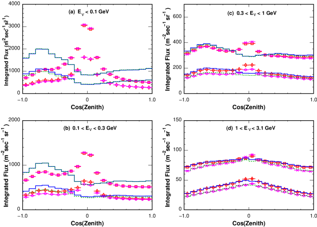
Figure 20: Comparison of three-dimensional and one-dimensional calculations of neutrino fluxes at Super-K Honda3D . Squares are for $\nu_{\mu}$, asterisks for $\bar{\nu}_{\mu}$, vertical diamonds for $\nu_{e}$, and horizontal diamonds for $\bar{\nu}_{e}$ for three dimensional calculation. The solid line histograms show the $\nu$ fluxes, and the dotted ones the $\bar{\nu}$ fluxes for the one dimensional calculation. The panels show four bins of neutrino energy: a) 0 –0.1 GeV, b) 0.1 – 0.3 GeV, c) 0.3 – 1 GeV, and d) 1 – 3.1 GeV. The fluxes are averaged over all azimuthal angles in 20 bands of $\cos(\theta)$ from $-1$ (straight up) to $+1$ (vertically downward moving).

7.1 Geometry of neutrino production

The most prominent feature of three-dimensional calculations is the neutrino flux enhancement near the horizon, as illustrated in Fig. 20 from Ref. Honda3D . This enhancement is a geometrical effect not present in the one-dimensional calculations. Fig. 20 compares 3D and 1D calculations specifically at Kamioka, where the angular dependence results from a complex combination of the physics of neutrino production, geomagnetic effects and geometry. Before discussing the figure in detail, a digression on the geometry of neutrino production will be helpful.

Lipari Lipari3D has given a detailed explanation of the origin of the excess of low energy neutrinos near the horizon in the 3D calculation, starting from an analysis in which all neutrinos are produced in a shell of constant altitude $h\sim 15$ km and geomagnetic effects are neglected. We follow his argument, generalizing it somewhat to display also the up-down symmetry of the neutrino flux that characterizes both the 3D and the 1D calculations in the absence of geomagnetic effects. Fig. 21 illustrates the detector $A$ at a distance $r_{A}\approx R_{\oplus}$ from the center of the earth surrounded by a shell of radius $r_{S}\approx R_{\oplus}+h$ centered around the Earth. Eventually, an integral has to be made over the production altitudes ($h$) of the neutrinos. Most neutrino production occurs in a band of altitude $10<h<20$ km, which is a thin shell compared to the radius of the Earth.

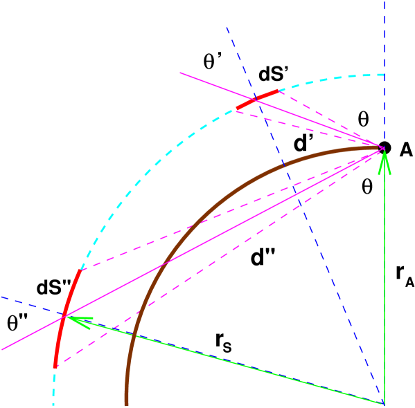
Figure 21: Geometry of atmospheric neutrino production (see text). The detector is at A, and we compare a neutrino entering from above the horizon at zenith angle $\theta$ with one entering from below the horizon at the same nadir angle. The angles $\theta^{\prime}=\theta^{\prime\prime}$ are the apparent local zenith angles in the production regions, indicated by the heavily shaded arcs.

We consider neutrino emission from two patches of the production shell with area $dS^{\prime}$ and $dS^{\prime\prime}$ above and below the horizontal at the same zenith and nadir angles, $\theta$ and with the same solid angle at the detector,

$$d\Omega=dS^{\prime}\cos\theta^{\prime}/(d^{\prime})^{2}=dS^{\prime\prime}\cos\theta^{\prime\prime}/(d^{\prime\prime})^{2}.$$ (15)

The distance to the patch above the horizon is $d^{\prime}=\ell$ and the distance to the patch below the horizon is $d^{\prime\prime}$, while the local zenith angles at the patches are $\theta^{\prime}$ and $\theta^{\prime\prime}$. By a geometrical construction one can show that the angles are related by

$$\cos\theta^{\prime}\;=\;\cos\theta^{\prime\prime}\;=\;\sqrt{1\,-\,(r_{A}/r_{S})^{2}\,\sin^{2}\theta}\;\geq\;\sqrt{1\,-\,(r_{A}/r_{S})^{2}}\;\approx\;0.07.$$ (16)

Next let $Y_{\nu_{i}}(E_{\nu},\Omega^{\prime})\;dE_{\nu}\;dS^{\prime}\;d\Omega^{\prime}$ be the number of neutrinos of type $i$ emitted from the patch $dS^{\prime}$ in energy interval [$E_{\nu},E_{\nu}+dE$] into the solid angle $d\Omega^{\prime}=d\cos\theta^{\prime}d\varphi^{\prime}$ centered at $\Omega^{\prime}=(\cos\theta^{\prime},\;\varphi^{\prime})$, per unit time. We represent the projected area of the detector as a function of zenith angle as ${\cal A}(\theta)$. Then, if the detector is up-down symmetric (i.e. ${\cal A}(\theta)={\cal A}(180^{\circ}-\theta)$), the solid angle subtended by the detector is ${\cal A}/(d^{\prime})^{2}$ above the horizon and ${\cal A}/(d^{\prime\prime})^{2}$ below. The corresponding rates of neutrinos through the detector are $Y_{\nu_{i}}(E_{\nu},\Omega^{\prime})\;dE_{\nu}\;dS^{\prime}\times{\cal A}/(d^{\prime})^{2}$ and $Y_{\nu_{i}}(E_{\nu},\Omega^{\prime\prime})\;dE_{\nu}\;dS^{\prime\prime}\times{\cal A}/(d^{\prime\prime})^{2}$ respectively. The differential rate from the patch above the horizon is

$${dN_{\nu_{i}}\over dE_{\nu}d\Omega d{\cal A}}={Y_{\nu_{i}}(E_{\nu},\Omega^{\prime})\;dE_{\nu}\;dS^{\prime}\times({\cal A}/(d^{\prime})^{2})\over dE_{\nu}(dS^{\prime}\cos\theta^{\prime}/(d^{\prime})^{2})({\cal A})}={1\over\cos\theta^{\prime}}Y_{\nu_{i}}(E_{\nu},\Omega^{\prime})$$ (17)

with the same result for the patch below the horizon. Eq. 15 has been used for $d\Omega$. Since the distances cancel and $\theta^{\prime\prime}=\theta^{\prime}$, the flux is symmetric from above and below the horizon no matter how complicated the dependence of $Y_{\nu}$ on angle, provided it is the same above and below the horizon (i.e. in the absence of geomagnetic effects, mountains, seasonal variations, etc.). To the extent that the detector response is also symmetric, the measured rates will be as well. The factor $1/\cos\theta^{\prime}$ in Eq. 17 is the origin of the enhancement near the horizontal in the 3D calculation. It comes from the expression 15 for the solid angle of the production region, and it is limited by the inequality in Eq. 16.

The relation between the yield for a patch of the production shell and the incident cosmic-ray flux is

$$Y_{\nu_{i}}(E_{\nu},\Omega^{\prime})\,=\,\int_{E_{cr}}\int_{\Omega_{cr}}\;\;[\eta_{\nu_{i}}(E_{\nu},\Omega^{\prime}:E_{cr},\Omega_{cr})\,]\times\;[(dN_{cr}/dE_{cr})\,\cos\theta_{cr}\,]\;d\Omega_{cr}dE_{cr},$$ (18)

where $\eta_{\nu_{i}}(E_{\nu},\Omega^{\prime}:E_{cr},\Omega_{cr})\,$ is the differential probability with which primary cosmic rays with energy $E_{cr}$ and arrival direction $\Omega_{cr}=(\cos\theta_{cr},\;\varphi_{cr})$ produce $\nu_{i}$ in the energy interval [$E_{\nu},E_{\nu}+dE$] and solid angle $d\Omega^{\prime}$. Apart from geomagnetic effects the flux of cosmic rays, $dN_{cr}/dE_{cr}$ $({\rm cm^{2}\cdot sr\cdot s\cdot GeV})^{-1}$, is isotropic. The factor $\cos\theta_{cr}$ in Eq. 18 is the projection of the isotropic flux onto the surface element $dS^{\prime}$ that is needed to obtain the rate at which primaries enter the production shell from a particular arrival direction.

As energy increases neutrino production becomes peaked in the forward direction ($\cos\theta_{cr}=\cos\theta^{\prime}$). In the high energy limit $\eta_{\nu_{i}}(E_{\nu},\Omega^{\prime})\rightarrow\eta_{\nu_{i}}(E_{\nu},\cos\theta^{\prime})\times\delta(\Omega^{\prime},\Omega_{cr})$, and we recover the one-dimensional approximation. Then $Y_{\nu_{i}}(E_{\nu},\Omega^{\prime})\propto\cos\theta^{\prime}$ and the horizontal enhancement in Eq. 17 is exactly canceled. For low energy neutrinos the deviation from the direction of the parent primary cannot be neglected and the cancellation is not complete. Eq. 14 sets the energy scale for the horizontal enhancement.

We return now to a discussion of the results displayed in Fig. 20. The intrinsic angular dependence of the one-dimensional calculation in the absence of the geomagnetic field is displayed in the left panel Fig. 3 in §2.1. When geomagnetic effects are unimportant, there is an excess of neutrinos near the horizon. At Super-K, however, there are regions of very high cutoff rigidity near the horizon, which leads to the suppression of low-energy neutrinos from near $\cos\theta=0$ for the 1D calculation shown by the line histograms in Fig. 20. The characteristic peaking near the horizon only appears again at Super-K for $E_{\nu}>1$ GeV (panel d in the figure). At this energy the three-dimensional effects are also negligible, and the 1D and 3D calculations agree. At lower energy, however, the flat behavior or suppression near $\cos\theta\sim 0$ is replaced with the horizontal peak characteristic of the correct 3D treatment.

The horizontal enhancement of the neutrino flux appears mainly at low energy and is therefore essentially impossible to detect because of the large angle between a low energy neutrino and the charged lepton that it produces in the detector Battistoni . The enhancement is significant only for lower energies and for $|\cos(zenith)|\approx 0.2$, within 12 degrees from the horizontal direction. Since the angle between the neutrino and the charged lepton it produces in the detector is expected to be $\sim$ 60 degree below 0.5 GeV, the horizontal enhancement cannot be resolved.

7.2 Pathlength distributions

     

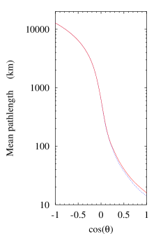
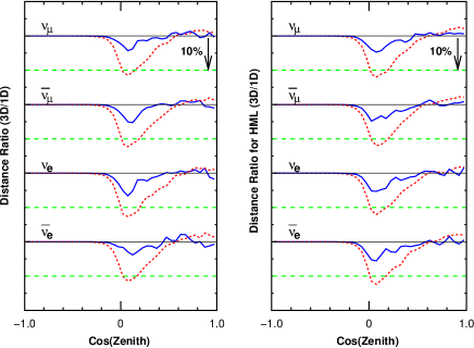
Figure 22: a) Mean pathlength of neutrinos with $0.3<E_{\nu}<2$ GeV in a 1D calculation pathlength . b) Ratio of the median path length in 3D calculation to that in 1D calculation both for Super-K and North America. Solid lines show the ratio for 1 GeV neutrinos, and dotted lines for 0.3 GeV neutrinos. $\cos\theta=1$ denotes the downward direction for neutrinos.

A key element of the interpretation of the evidence for oscillations is the pathlength-dependence of the atmospheric neutrino beam. To a first approximation, the distribution is a delta function equal to the distance from the detector along the direction of the neutrino to a shell at approximately 15 kilometers altitude. The next step was to calculate the pathlength distribution corresponding to the distribution of production depths still assuming the neutrino is along the direction of the primary cosmic ray that produced it pathlength . This is the approach used so far in the analysis of the Super-K data, and the mean value of the pathlength in the 1D calculation pathlength is shown in Fig. 22a. What is still lacking is a treatment of the pathlength distribution with the full three-dimensional geometry. In particular, the excess of low energy neutrinos near the horizon in the 3D calculation arises in part from neutrinos produced closer to the detector than neutrinos from the same direction in the 1D calculation. This is possible because the more nearly vertical nearby primaries can contribute neutrinos at zenith angles that would require larger pathlengths if the primary and the neutrino direction were the same. The nearby case just described is not fully compensated by larger angle primaries producing smaller angle neutrinos. This is a consequence of the $\cos\theta_{cr}$ projection factor in Eq. 18.

We compare the path length calculated in the 1D and 3D calculations, converting the median production height to the path length by a simple relation:

$$\ell=\sqrt{(h^{2}+2R_{\oplus}h)+(R_{\oplus}\cos\theta)^{2}}-R_{\oplus}\cos\theta~{}~{}.$$ (19)

We show the ratio of the two path lengths (3D$/$1D) as a function of $\cos(\theta)$ in Fig. 22 from Ref. Honda3D . In this comparison an average over azimuth has been made. Near the horizon the production distance of 0.3 GeV neutrinos is $\sim$ 10 % smaller for 3D calculation than for 1D. For 1 GeV the difference decreases to ${\buildrel<\over{\sim}}$ 5 %. As there is not a visible difference between the plots for Kamioka and for high-latitude North America, we may conclude that there is almost no geomagnetic latitude dependence of the path length differences.

8 Atmospheric muons

In this section we review the use of muon flux as a constraint on the atmospheric neutrino calculations. We focus on the low energy region, where pions give the dominant contribution to neutrinos as well as to muons.

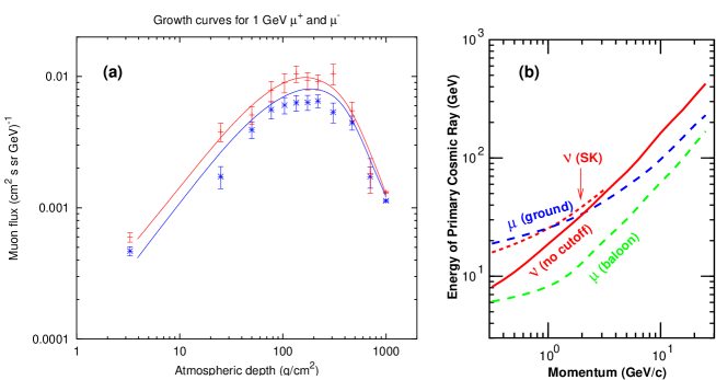
Figure 23: a. Growth curve of muons. The data are those of Ref. CAPmu and lines are 3D calculations from Ref. Engmu . b. Median primary energy per nucleon for muons and neutrinos (see text).

Fig. 23a shows the growth curve of the vertical atmospheric muon flux for $E_{\mu}\approx 1$ GeV as a function of atmospheric depth $X\,({\rm gm/cm}^{2})$. The flux increases with depth from top of atmosphere down to $X\sim 100\;{\rm g/cm^{2}}$. For $X\ll\lambda_{N}\approx 80$ gm/cm² (where $\lambda_{N}$ is the nucleon interaction length) the increase is proportional to $X$. In the region of 100–200 g/cm², the attenuation of the primary cosmic rays and the increase of the column density compensate each other, and the muon flux is almost constant. Below 200 g/cm², the muon flux decreases rapidly as muon production decreases and muon decay and energy-loss become important. Since decay probability and the importance of energy loss depend on energy, the growth curve depend somewhat on energy, but the qualitative behavior is unchanged.

Fig. 23b shows the median primary energy per nucleon for vertical muons (dashed lines) and neutrinos averaged over all angles (heavy solid and dotted curves). Comparison of response curves for muons at the ground and at float altitude (typically $<5$ g/cm²) shows the effect of muon energy loss in the atmosphere. Muons typically lose $\approx 1.8$ GeV propagating through the atmosphere, and most muons produced with this energy decay before reaching the ground. On the other hand, high in the atmosphere the muons have not lost energy and are closer in energy to the primaries. For neutrinos, the solid line is for Kamioka site, and the dotted line is the result that would be obtained in the absence of a geomagnetic cutoff. The response curve for north America or Gransasso would be between the solid and dashed lines. Both muon charges ($\mu^{+},\mu^{-}$), and all neutrinos species ($\nu_{\mu}$, $\bar{\nu}_{\mu}$, $\nu_{e}$, $\bar{\nu}_{e}$) were summed for these curves.

Measurements of muons in the cosmic radiation date back to the early days of the subject. A wealth of information on this and other relevant topics is to be found in the comprehensive work of Grieder Grieder . There is also a recent study of muons with $E\lower 3.01385pt\hbox{${\buildrel>\over{\sim}}$}10$ GeV at ground level in which the authors have corrected the data for different observing conditions Hebbeker . A thorough summary is also given in Ref. Naumov . In the past decade, several groups have measured the flux of muons on the ground and during ascent to float altitude MASS ; CAPmu ; HEAT ; bess-sanuki , and several groups Hondanew ; Fior ; Liu ; Engmu ; Battistonimu have compared their calculations to some or all of this data.

Several issues arise in comparing calculations with muon data. One is whether to use the primary spectrum measured during the muon flight (if available) or to use some kind of best fit or preferred spectrum. For example, Battistoni et al. Battistonimu get generally good agreement with the Caprice muon data CAPmu using the primary spectrum of Ref. AGLS , which is higher than that measured the Caprice detector CAPRICE at the same time as the muon measurement was made. They note that their normalization would have been generally lower than the muon data had they used the Caprice primary spectrum. On the other hand the CAPRICE primary spectrum is used in Ref. Engmu to obtain the results shown in Fig. refFig-mu-growtha. That calculation uses the interaction model Target 2.1, which gives higher neutrino fluxes at Soudan than the calculation with FLUKA Battistoni . Since the muon fluxes are also measured with no geomagnetic cutoff, the origin of the difference between these two results is presumably the same–a difference in pion production in interactions of $E_{N}<10$ GeV.

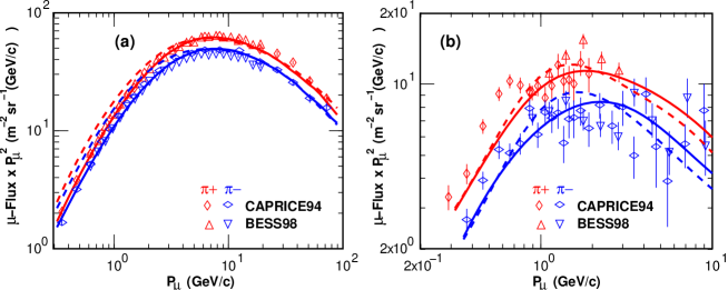
Figure 24: The flux of positive and negative muons observed at Lynnlake and corresponding calculations. Left panel refers to measurements at the ground CAPground ; bess-motoki ; right panel to float altitude CAPmu ; bess-sanuki . Thick solid and dotted lines show the positive and negative pion spectra calculated based on Dpmjet3 interaction model Hondanew . Thin solid and dotted lines show the positive and negative pion spectra calculated based on Fritiof 1.6 interaction model as used in Honda .

Fig. 24 Hondanew compares calculations with data of two measurements both made in summer at Lynn Lake in Northern Canada where the geomagnetic cutoff is negligible. The Caprice muon data CAPmu ; CAPground was obtained in 1994, while the BESS muon data is a compilation of observations made in 1997, 1998, and 1999 bess-sanuki ; bess-motoki . The neutron monitor count rates for both experiments (averaged over the three dates in the case of BESS) are similar to that of 1998 when BESS and AMS measured the primary cosmic ray spectrum (see Fig. 8). The left panel shows a comparison with the muon fluxes at the ground. The comparison at float altitude is shown on the right. It is noteworthy that the two measurements of the muon flux at the ground are in better agreement with each other than the corresponding two measurements of the primary proton spectrum CAPRICE ; BESS . Despite relatively long exposures at float altitude, the statistics are poor because of the low flux.

Finally, we note that it may also be useful to compare high-statistics ground level measurements made a different geomagnetic locations. Ref. CAPground compares a measurement at Lynn Lake ($R_{c}\approx 0.5$ GV) with one at Ft. Sumner ($R_{c}\approx 4.2$ GV). Ref. bess-motoki compares their ground level measurement at Lynn Lake with a measurement at Tsukuba, Japan, which has a higher cutoff of $11.4$ GV. The charge ratios measured at the locations with a significant geomagnetic cutoff fall below those measured at Lynn Lake for $E_{\mu}<1$ GeV. This is expected qualitatively for several reasons. Helium is relatively more important at high cutoff because the energy per nucleon at cutoff is approximately half that of protons, and helium produces a charge ratio of unity. In addition, when the cutoff is high the low energy muons must come more from the central region of interactions above cutoff, and the charge ratio is lower in the central region. Finally, there is also some contribution from the east-west effect since vertical muons of opposite sign are bent in opposite directions Utah .

We summarize this section as follows. Because of decay and energy loss, low energy muons at the ground carry less information about neutrino production than those at high altitude where most of the neutrinos are produced. In addition, the variation of atmospheric structure from barometric and seasonal changes is significant and must be accounted for. At float altitude, the muons reflect rather directly the properties of pion production and primary cosmic-ray intensity since only one interaction is involved, but this is above the depth where most muons and neutrinos are produced and the flux is very low. On the other hand, the peak of the grown curve has so far been studied only during ascent where the balloon rises rapidly through the atmosphere, so that statistical and systematic uncertainties are larger than on the ground or at float. In addition, at all altitudes, the fraction of $\sim$GeV muons passing through a detector is always much smaller than the number of muons that were produced above it Engmu . Thus calculating the muon flux is more delicate than calculating the neutrino flux which is an integral over all depths.

9 Uncertainties in the Calculated Neutrino Fluxes

Remaining uncertainties in the flux of atmospheric neutrinos come mainly from the primary spectrum and from the treatment of hadronic interactions. In addition, there remain uncertainties of a technical nature related to remaining approximations in present calculations. The uncertainty in the signal for a given experiment depends on its response function, which determines the distribution of primary energy responsible for the signal. Key examples are shown in Fig. 5.

9.1 Uncertainties from primary spectrum

An estimate spectrum of the uncertainty in the primary spectrum in the light of recent measurements by BESS BESS and AMS AMS is $\pm 5$% below $100$ GeV/nucleon increasing to $\pm 10$% at $10$ TeV/nucleon. This is based on a fit (Eq. 10 to BESS and AMS data alone and assumes a power-law to extrapolate beyond the upper range of those measurements ($\approx 100$ GeV).

A more proper estimate of the uncertainty in the primary spectrum uses all valid measurements, including those with larger quoted uncertainties, to estimate the systematic uncertainty in the primary spectrum. Fig. 6 shows a collection of measurements for protons and helium. Although there are now several recently reported measurements below 100 GeV, there is a striking lack of recent data in the TeV range, important for $\nu$-induced upward muons. Even assuming the high-energy data should be renormalized down to connect with the low-energy data, the measurements cover a range of $\pm 20$% below 100 GeV and $\pm 30$% above.

9.2 Uncertainties from hadronic interactions

It is more difficult to quantify the uncertainties due to hadronic interactions. As shown in Fig. 16, large regions of phase space are not measured, and models are needed to interpolate and extrapolate into the unmeasured regions. Study of Fig. 15 show a scatter of 20-25% even if we consider the data of Ref. Lundy as an outlier. On the other hand, this treats the different inclusive cross sections as independent of each other, when in fact they are interrelated by energy conservation.

Combining the systematic uncertainties in primary spectrum and in pion production as if they were independent statistical uncertainties, we would therefore estimate an overall theoretical uncertainty of $\pm$20 to 25% in the energy range relevant for contained neutrino interactions and somewhat larger at higher energy.

9.3 Other sources of uncertainty

Calculations usually assume a spherical earth with the surface at sea level. When parent mesons enter the ground before decaying they loose energy rapidly by ionization or the nuclear interactions and produce only very low energy neutrinos. Therefore, when there is a high mountain over the neutrino detector, the neutrino flux is reduced to some extent. The effect is negligible except near the vertical and then only for decay products of muons. The reduction has been estimated Honda2000 as a 2–3 % effect for $\nu_{e}$ in the 10-100 GeV range due to the Ikenoyama mountain over Super-Kamiokande, which has a peak at approximately 1300 m above sea level.

Calculations are normally made for an average atmosphere. While pressure and seasonal variations have a noticeable effect on surviving muon fluxes at the ground, they are small for for neutrinos. Variations at the per cent level have been estimated in Ref. Honda2000 .

9.4 Comparison to measurements

A consistent picture emerges from comparison of a variety of data to calculations of the flux of atmospheric neutrinos. All analyses emphasize comparison to ratios, which include $\nu_{e}/\nu_{\mu}$ and up/down for contained events and stopping/throughgoing and vertical/horizontal for neutrino-induced upward muon. As a consequence, an offset in normalization does not affect the conclusions about oscillations, which are robust.

     

Figure 25: Sub-GeV neutrino spectrum.

Nevertheless, it is also interesting and informative to compare the measured neutrino flux as directly as possible in an absolute fashion with the calculations. Fig. 25 compares the neutrino fluxes measured at Super-K with the two calculations Honda ; AGLS that have been used extensively as input to the detector simulation. The comparisons are made as a function of visible energy by the Super-K group Kajita-private . The magnitudes are consistent with what is expected for oscillations in this energy range that involve $\nu_{\mu}$ and $\nu_{\tau}$ but not $\nu_{e}$; namely, there is a deficit of $\nu_{\mu}$, whereas the measured flux of electron neutrinos is consistent with the calculation.

Systematic comparisons of more recent calculations with data are not yet available. Based on comparisons between old and new calculations such as those shown in Fig. 19, however, we expect that the new calculations will give significantly lower predicted neutrino fluxes. In Refs. Hamburg ; FLUKA this will be a consequence of lower pion production, whereas in the case of Ref. Hondanew the primary spectrum is lower than before Honda . We expect the predictions may be reduced by as much as 15 to 20%, without changing the ratios significantly. Possible resolutions include uncertainties in the neutrino cross sections Sartogo ; Nuint01 or systematic uncertainty in primary spectrum (despite the agreement between BESS BESS and AMS AMS or higher pion production (despite new calculations) or some combination of the above.

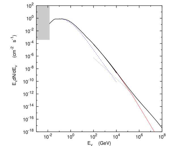
Figure 26: Global view of the neutrino spectrum: vertical flux of $\nu_{\mu}+\bar{\nu}$ (heavy solid line); $\nu_{e}+\bar{\nu}_{e}$ (dashed line); prompt neutrinos (dotted line); $\nu_{\mu}+\bar{\nu}$ from pions and kaons (thin solid line at high energy).

10 Global view of the neutrino spectrum

Figure 26 is a global view of the omnidirectional neutrino flux from the MeV range up to 100 PeV. Below 15-18 MeV solar neutrinos dominate, as indicated by the shaded region. It has been pointed out SNe1 ; SNe2 ; SNe that there is potentially a window between $\sim 15$ and $50$ MeV where the accumulated diffuse flux from supernovae in the Universe could be comparable to or larger than the flux of atmospheric neutrinos.

The heavy solid line shows the flux of atmospheric $\nu_{\mu}+\bar{\nu}_{\mu}$ integrated over all directions. The dotted lines show the flux of $\nu_{e}+\bar{\nu}_{e}$. Where geomagnetic effects are important (below several GeV), we show the integrated flux at Kamioka. With the discovery of oscillations, the flux of muon neutrinos is suppressed in the energy region below 100 GeV. We used the Super-K oscillation parameters evidence assuming $\nu_{\mu}\leftrightarrow\nu_{\tau}$ to relate the production spectrum of $\nu_{\mu}+\bar{\nu}_{\mu}$ as calculated in Ref. AGLS to the flux at the detector. Thus for $E_{\nu}<10$ GeV the $\nu_{\mu}/\nu_{e}$ ratio decreases toward 1.

For $E_{\nu}\sim 100$ GeV and beyond, most neutrinos come from decay of kaons until the energy is so high that prompt neutrinos dominate. The dotted line at higher energy is the flux of prompt neutrinos ($\nu_{e}+\bar{\nu}_{e}\approx\nu_{\mu}+\bar{\nu}_{\mu}$) from decay of charm, as estimated in the RQP model of Ref. Bugaev . In this model, the charm crossover is at $\sim 3$ TeV for electron neutrinos and around $100$ TeV for muon neutrinos. The thinner (lower) solid line above $100$ TeV is the non-prompt contribution to the flux of $\nu_{\mu}+\bar{\nu}_{\mu}$. In the TeV region and above the atmospheric neutrinos become a foreground for high energy astrophysical neutrinos, and the uncertainty in the level of prompt neutrinos becomes an important consideration in this context.

11 Acknowledgments

We are grateful to Giles Barr, Giuseppe Battistoni, Ralph Engel, Frank Jones, T. Kajita, K. Kasahara, Paolo Lipari, S. Midorikawa, Teresa Montaruli, T. Sanuki and Todor Stanev for their assistance and advice as we prepared this review. The data plotted in Fig. 8 are from research supported by National Science Foundation Grant ATM-9912341 at the University of Chicago. One of us (TKG) gratefully acknowledges the hospitality of the Institute for Cosmic Ray Research where most of this review was prepared. The work of TKG is supported in part by the U.S. Department of Energy under DE-FG02 91ER 40626.

12 LITERATURE CITED

References

- (1) Markov MA, in Proc. 1960 Annual Int. Conf. on High Energy Physics at Rochester (ed. Sudarshan ECG, Tinlot JH, & Melissinos AC. ) p578 (1960)
- (2) Markov MA, Zheleznykh IM. Nuclear Physics 27:385 (1961)
- (3) Greisen K, Ann. Rev. Nucl. Science 10:63 (1960)
- (4) Achar CV, et al. Phys. Lett. 18:196 and 19:78 (1965)
- (5) Reines F, et al. Phys. Rev. Lett. 15:429 (1965)
- (6) Fukuda Y, et al. Phys. Rev. Lett. 81:1562 (1998)
- (7) Fukuda S, et al. Phys. Rev. Lett. 85:3999. (2000)
- (8) Ahmad QR, et al. Phys. Rev. Lett. 87:071301 (2001)
- (9) Haines TJ, et al. Phys. Rev. Lett. 57:1986 (1986)
- (10) Hirata KS, et al. Phys. Lett. B205:416 (1988)
- (11) Berger Ch, et al. Phys. Lett. B245:305 (1990)
- (12) Casper D, et al.Phys. Rev. Lett. 66:2561 (1991)
- (13) Becker-Szendy R, et al. Phys. Rev. D46:3720 (1992)
- (14) Hirata KS, et al. Phys. Lett. B280:146 (1992)
- (15) Beier EW, et al. Phys. Letters B283:446 (1992)
- (16) Allison WWM, et al. Phys. Lett. B391:491 (1997) and B449:137 (1999)
- (17) Fukuda Y, et al. Phys. Lett. B335 (1994) 237.
- (18) Lipari P. in Neutrino Oscillations and their Origin (ed. Suzuki Y, Nakahata M, Shiozawa M, & Kaneyuki K. Universal Academy Press, 2000) p. 65
- (19) Ambrosio M, et al. Phys. Lett. B517:59 (2001) and B434:451 (1998)
- (20) Fukuda Y, et al. Phys. Rev. Lett. 82:2644 (1999)
- (21) Ambrosio M, et al. Phys. Lett. B478:5 (2000)
- (22) Fukuda Y, et al. Phys. Lett. B467:185 (1999)
- (23) Kajita T, Totsuka Y. Revs. Mod. Phys. 73:85 (2001)
- (24) Jung C-K, Kajita T, Mann A, McGrew C, Ann. Revs. Nucl. Part. Sci. 51:451 (2001)
- (25) Balkanov VA, et al. Nucl. Phys. B Proc. Suppl. 91:438 (2001)
- (26) Andres E, et al. Astropart. Phys. 13:1 (2000)
- (27) Bottai S, et al. Nucl. Phys. B Proc. Suppl. 85:153 (2000)
- (28) Thompson LF, et al. Nucl. Phys. B Proc. Suppl. 91:431 (2001)
- (29) http://nemoweb.lns.infn.it/
- (30) Goldschmidt A, et al. Proc. 27th Int. Cosmic Ray Conf. 3:1237 (2001)
- (31) Zatsepin GT, Kuz’min VA. Soviet Phys. JETP 14:1294 (1961)
- (32) Agrawal V, Gaisser TK, Lipari P, & Stanev T. Phys. Rev D53:1314 (1996)
- (33) Engel R, Gaisser TK, Lipari P, & Stanev T, Proc. 27th Int. Cosmic Ray Conf. 4:1381 (2001)
- (34) Battistoni G, et al. Astropart. Phys. 12:315 (2000) and http://www. mi. infn. it/ battist/neutrino. html
- (35) Honda M, Kajita T, Kasahara K, & Midorikawa S. Phys. Rev. D52:4985 (1995)
- (36) Honda M, Kajita T, Kasahara K, & Midorikawa S. Proc. 27th Int. Cosmic Ray Conf. 3:1162 (2001)
- (37) Volkova LV. private communication (1988)
- (38) Zatsepin GT, Kuz’min VA. Soviet Phys. JETP 12:1171 (1961)
- (39) Perkins DH. Nucl. Phys. B399:3 (1993)
- (40) Perkins DH. Astropart. Phys. 2:249 (1994)
- (41) Gaisser, TK. Cosmic Rays and Particle Physics (Cambridge University Press, 1992)
- (42) Lipari P. Astropart. Phys. 1:195 (1993)
- (43) Gaisser TK. Astropart. Phys. 16:285 (2002)
- (44) Compton AH, Getting IA. Phys. Rev. 47:817 (1935)
- (45) Cutler DJ, Groom DE. Astrophys. J. 376:322 (1991)
- (46) Nagashima K, Fujimoto K, Jacklyn RM. J. Geophys. Res. 103:17429 (1988)
- (47) Webber WR, Golden RL, Stephens SA. Proc. 20th Int. Cosmic Ray Conf. 1:325 (1987)
- (48) Seo E-S, et al. Astrophys. J. 378:763 (1991)
- (49) Pappini P, et al. Proc. 23rd Int. Cosmic Ray Conf. 1:579 (1993)
- (50) Bellotti R, et al. Phys. Rev. D60:052002 (1999)
- (51) Boezio M, et al. Astrophys. J. 518:457 (1999)
- (52) Menn W, et al. Astrophys. J. 533:281 (2000)
- (53) Sanuki T, et al. Astrophys. J. 545:1135 (2000)
- (54) Alcarez J, et al. Phys. Lett. B490:27 (2000)
- (55) Ryan MJ, Ormes JF, Balasubrahmanyan VK. Phys. Rev. Lett. 28:985, E1497 (1972)
- (56) Asakamori K, et al. Ap. J. 502:278 (1998)
- (57) Ivanenko IP, et al. Proc. 23rd Int. Cosmic Ray Conf. 2:17 (1993)
- (58) Apanasenko AV, et al. Astropart. Phys. 16:13 (2001)
- (59) Kawamura Y, et al. Phys. Rev. D40:729 (1989) (1989)
- (60) T. K. Gaisser, M. Honda, P. Lipari & T. Stanev, Proc. 27th Int. Cosmic Ray Conf. (2001) 1643.
- (61) Stanev T. Private communication.
- (62) The Heliosphere at Solar Minimum (ed. Page DE, Marsden RG, ) Pergamon Press, (1997)
- (63) Simpson J. Phys. Rev 73:1389 (1948)
- (64) Clem JM, Dorman LI. Space Science Reviews 93:335 (2000)
- (65) http://www.bartol.udel.edu/ neutronm/
- (66) http://ulysses.uchicago.edu/NeutronMonitor/Misc/neutron2.html
- (67) Nagashima K, et al. Nuovo Comento C12:173 (1989)
- (68) Lipari P. private communication (2001)
- (69) Gleeson LJ, Axford WI. Astrophys. J. 154:1011 (1968)
- (70) Asaoka Y, et al. Phys. Rev. Letters 88:51101 (2002)
- (71) Störmer C. Z. Astrophys. 1:237 (1930)
- (72) Alpher RA. J. Geophys. Res. 55:437 (1950)
- (73) http://nssdc. gsfc. nasa. gov/space/model/models/igrf. html
- (74) Lipari P, Stanev T. Proc. 24th Int. Cosmic Ray Conf. 1:516 (516)
- (75) Johnson TH, Phys. Rev. 43:834 (1933)
- (76) Alvarez LW, & Compton A. H. Phys. Rev. 43:835 (1933)
- (77) Futagami T, et al. Phys. Rev. Lett. 82:5192 (1999)
- (78) Lipari P, Stanev T & Gaisser TK, Phys. Rev. D58:073003 (1998)
- (79) Lipari P. Astropart. Phys. 14:153 (2000)
- (80) Alcarez J, et al. Phys. Lett. B472:215 (2000)
- (81) Treiman SB. Phys. Rev. 53:957 (1953)
- (82) Barwick SW, et al. J. Geophys. Res. 103:4817 (1998)
- (83) Verma SD, J. Geophys. Res. 72:915 (1967)
- (84) Derome L, et al. Phys. Lett. B489:1 (2000)
- (85) Lipari P. Astropart. Phys. 16:295 (2002)
- (86) Zuccon P, et al. astro-ph/0111111
- (87) Lipari P, Astropart. Phys. 14:171 (2000)
- (88) Honda M, Kajita T, Kasahara K, Midorikawa S. Phys. Rev. D64:053011 (2001)
- (89) Ralph Engel, private communication.
- (90) Glauber RJ, Matthiae G. Nucl. Phys. B21:135 (1970)
- (91) Dersch U, et al. Nucl. Phys. B 579:277 (2000)
- (92) Engel J, Gaisser TK, Lipari P, Stanev T. Phys. Rev. D46:5013 (1992)
- (93) Cho Y, et al. Phys. Rev. D4:1967 (1971)
- (94) Sanford JR, Wang CL. BNL, AGS internal report (unpublished, 1967); Wang, CL. Phys. Rev. Lett. 25:1068, 1536(E) (1970)
- (95) Allaby JV, et al. CERN Yellow Report 70-12 (1970)
- (96) Eichten T, et al. Nucl. Phys. B44:333 (1972)
- (97) Abbott T, et al. Phys. Rev. D45:3906 (1992)
- (98) Lundy RA, et al. Phys. Rev. Lett. 14:504 (1965)
- (99) Engel R, Gaisser TK, & Stanev T, Phys. Lett. B472:113 (2000)
- (100) Ferrari A. Physica Medica Vol. XVII, Suppl. 1.
- (101) G. Battistoni, private communication.
- (102) Roesler S, Engel & R, Ranft J. Proc. 27th Int. Cosmic Ray Conf. 1:439 (2001), Phys. Rev. D57:2889 (1998), D55:6957 (1997)
- (103) Nilsson-Almqvist & B, Stenlund E. Comput. Commun. 43:387 (1987)
- (104) Tan LC, & Ng LK. J. Phys. G: Nucl. Phys. 9:1453 (1983)
- (105) Costa CGS. Astropart. Phys. 16:193 (2001)
- (106) Volkova LV, Fulgione W, Galeotti P, & Saavedra O. Nuovo Cimento C10:465 (1987)
- (107) Thunman M, Ingelman G, & Gondolo P. Astropart. Phys. 5:309 (1996)
- (108) Pasquali L, Reno MH, & Sarcevic I. Phys. Rev. D59:034020 (1999)
- (109) Gaisser TK, & Halzen F. Phys. Rev. D11:3157 (1973)
- (110) Bugaev EV, et al. Phys. Rev. D58:054001 (1998)
- (111) Tserkovnyak Y, Komar RJ, Nally CW, & Waltham CE. Proc. 27th Int. Cosmic Ray Conf. 3:1196 (2001)
- (112) Fiorentini G, Naumov VA, & Villante FL. Phys. Lett. B510:173 (2001) and Proc. 27th Int. Cosmic Ray Conf. 3:1218 (2001)
- (113) Wentz J, et al. Proc. 27th Int. Cosmic Ray Conf. 3:1167 (2001) and private communication
- (114) Liu Y, Derome L. & Buénerd M, Proc. 27th Int. Cosmic Ray Conf. 3:1033. (2001)
- (115) Plyaskin V, Phys. Lett. B516:213 (2001)
- (116) Gaisser TK, & Stanev T. Phys. Rev. D57:1977 (1998)
- (117) Boezio M, et al. Phys. Rev. D62:032007 (2000)
- (118) Engel R, Gaisser TK, & Stanev T. Proc. 27th Int. Cosmic Ray Conf. 3:1029 (2001)
- (119) Grieder PKF. Cosmic Rays at Earth, Researcher’s Reference Manual and Data Book (Elsevier Science, 2001)
- (120) Hebbeker T, & Timmermans C. Astropart. Phys. (to be published, hep-ph/0102042)
- (121) Naumov VA. hep-ph/0201310
- (122) Coutu S, et al. Phys. Rev. D62:032001 (2000)
- (123) Sanuki T, et al. Proc. 27th Int. Cosmic Ray Conf. 3:950 (2001)
- (124) Motoki M, et al. Proc. 27th Int. Cosmic Ray Conf. 3:927 (2001)
- (125) Battistoni G, Ferrari A, Montaruli T, & Sala PR. Astropart. Phys. (to be published; hep-ph/0107241)
- (126) Kremer J, et al. Phys. Rev. Lett. 83:4241 (1999)
- (127) Stanev T, Coutu S, Gaisser TK, & Barr G. Proc. 26th Int. Cosmic Ray Conf. 2:96 (1999)
- (128) Honda M. Neutrino Oscillation and their origin, Universal Academy Press (ed. Suzuki Y, Nakahata M, Shiozawa M, & Kaneyuki K. Universal Academy
- (129) Kajita T. Private communication
- (130) Lipari P, Lusignolo M, Sartogo F. Phys. Rev. Letters 74:4384 (1995)
- (131) Proc. Workshop on Neutrino-Nucleus Interactions in the Few GeV Region, Nucl. Phys. B (Proc. Suppl) (to be published, 2000) http://neutrino.kek.jp/nuint01/ December 2001
- (132) Krauss LM, Glashow SL, Schramm DN. Nature 310:191 (1984)
- (133) Bisnovatyi-Kogan GS, Seidov SF. Ann NY Acad. Sci 422:319 (1984)
- (134) Totani T, Sato K, Yoshii Y. Ap. J 460:303 (1996)