Neutrino Mass Matrix Running for Non-Degenerate See-Saw Scales

Abstract

We consider the running of the neutrino mass matrix in the Standard Model and the Minimal Supersymmetric Standard Model, extended by heavy singlet Majorana neutrinos. Unlike previous studies, we do not assume that all of the heavy mass eigenvalues are degenerate. This leads to various effective theories when the heavy degrees of freedom are integrated out successively. We calculate the Renormalization Group Equations that govern the evolution of the neutrino mass matrix in these effective theories. We show that an appropriate treatment of the singlet mass scales can yield a substantially different result compared to integrating out the singlets at a common intermediate scale.

TUM-HEP-459/02

, , and

1 Introduction

The discovery of neutrino masses requires an extension of the Standard Model (SM) or the Minimal Supersymmetric Standard Model (MSSM), which may involve right-handed neutrinos, or more generally gauge singlets. Since there are no protective symmetries, these singlets are usually expected to have huge explicit (Majorana) masses. This leads to the see-saw mechanism [1], which provides a convincing explanation for small neutrino masses. This scenario can be realized in many Grand Unified Theories (GUT’s) and their supersymmetric counterparts. For instance, left-right symmetric models and $\text{SO}(10)$ GUT’s include singlet neutrinos, which can get huge masses in several ways, e.g. by a Higgs in a suitable representation or radiatively. Furthermore, additional singlets may exist, which can also be involved in the see-saw mechanism.

It is often assumed that all heavy singlet mass eigenvalues are degenerate. However, in all the models a large hierarchy of the singlet masses is possible. Note that such a hierarchical spectrum may even show up if all elements of the singlet mass matrix are of the same order. Democratic mass matrices, where this is the case due to discrete symmetries, are an example. Another argument for a non-degenerate spectrum follows from assuming a neutrino Yukawa matrix $Y_{\nu}$ which is proportional to the diagonalized charged lepton Yukawa matrix $Y_{e}$, i.e. the relation $Y_{\nu}=c_{\nu}Y_{e}\approx c_{\nu}\operatorname{diag}(10^{-2},10^{-3},10^{-5})$ holds with a constant real number $c_{\nu}$. If the neutrino masses are degenerate and of the order $1\,\mathrm{eV}$, the see-saw relation $\kappa=\frac{4}{v^{2}_{\mathrm{EW}}}M_{\nu}=2Y_{\nu}^{T}M^{-1}Y_{\nu}$ for the neutrino mass matrix $M_{\nu}$ allows to determine the singlet mass matrix $M$. Mixings do not significantly alter this picture, since e.g. bimaximal mixing can be accomplished by small modifications of a degenerate $M_{\nu}$ of the order $10^{-2}\,\mathrm{eV}$ or $10^{-3}\,\mathrm{eV}$, respectively. Taking for example $c_{\nu}=100$, the mass eigenvalues of $M$ are of the order $10^{7}\,\mathrm{GeV}$, $10^{11}\,\mathrm{GeV}$ and $10^{13}\,\mathrm{GeV}$ for the case at hand. It is therefore conceivable that there may be an even larger hierarchy in $M$ than in the charged lepton Yukawa matrices. Altogether, there are thus good reasons to study the effects of a non-degenerate or even hierarchical singlet mass spectrum.

In this paper, we calculate the Renormalization Group Equations (RGE’s) for the evolution of the neutrino mass matrix from the GUT scale to the electroweak or SUSY breaking scale. We consider the case where the SM and the MSSM are extended by an arbitrary number of heavy singlets which have explicit (Majorana) masses with a non-degenerate spectrum. Hence, to study the RG evolution of neutrino masses several Effective Field Theories (EFT’s), with the singlets partly integrated out, have to be taken into account. Below the lowest mass threshold, the neutrino mass matrix is given by the effective dimension 5 neutrino mass operator in the SM or MSSM, respectively. The corresponding RGE’s were derived in [2, 3, 4, 5, 6].

2 Effective Theories from Integrating Out Singlet Neutrinos

Consider the SM or the MSSM with $n_{G}$ additional sterile neutrinos. The eigenvalues of the mass matrix $M$, i.e. the masses of the mass eigenstates $\{N_{\mathrm{R}}^{1},\dots,N_{\mathrm{R}}^{n_{G}}\}$, have a certain spectrum, $M_{1}\leq M_{2}\leq\dots\leq M_{n_{G}}$. We will consider the general case that this spectrum is non-degenerate. Successively integrating out the heavy sterile neutrinos at the thresholds $M_{i}$ results in effective theories, valid in certain energy ranges as depicted in figure 1.

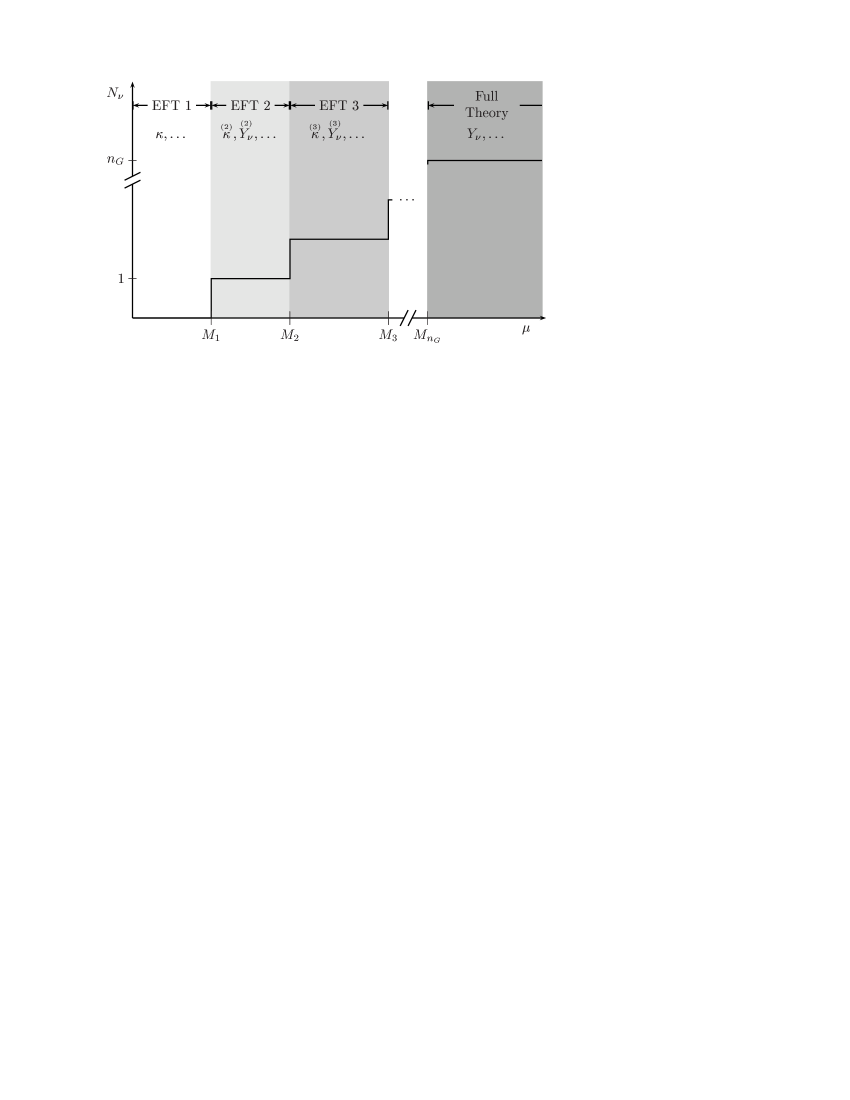
Figure 1: Illustration of the ranges of the different theories. The EFT’s emerge from successively integrating out the heavy fields. “EFT 1” corresponds to the SM or MSSM with additional dimension 5 mass operators for neutrino masses. “Full Theory” refers to the SM or MSSM, extended by $n_{G}$ gauge singlets. The meaning of the variables is explained in the text.

Before we calculate the RGE’s in the various theories, let us specify the modifications in the Lagrangians due to the appearance of the heavy neutrinos. In the SM above the highest mass threshold (“Full Theory” in figure 1), the kinetic and mass term as well as the Yukawa interaction for the singlet neutrinos $N_{\mathrm{R}}^{i}$, $i\in\{1,\dots,n_{G}\}$, are added:

$$\mathscr{L}_{\mathrm{N}}=\overline{N_{\mathrm{R}}^{i}}(i\gamma^{\mu}\partial_{\mu})N_{\mathrm{R}}^{i}+\left(-\frac{1}{2}\overline{N_{\mathrm{R}}^{i}}M_{ij}N^{\mathrm{C}j}_{\mathrm{R}}-(Y_{\nu})_{if}\overline{N_{\mathrm{R}}^{i}}\widetilde{\phi}^{\dagger}\ell^{f}_{\mathrm{L}}+\text{h.c.}\right)\;,$$ (1)

where $N_{\mathrm{R}}^{\mathrm{C}}:=(N_{\mathrm{R}})^{\mathrm{C}}$ is the charge conjugate of $N_{\mathrm{R}}$. $f\in\{1,\dots,n_{F}\}$ are flavour indices, $\ell_{\mathrm{L}}^{f}$ are the SU(2)_L-doublets of leptons, $\phi$ is the Higgs doublet, and $\widetilde{\phi}:=i\sigma^{2}\phi^{*}$. Summation over repeated indices is implied throughout the paper. For the calculation of the RGE’s, we will work in a basis in which the Majorana mass matrix $M$ is diagonal.

In the MSSM, the additional gauge singlet Weyl spinors $\nu^{\mathrm{C}i}$, which correspond to the right-handed Dirac spinors $N_{\mathrm{R}}^{i}$, and their superpartners are components of the chiral superfields ^Ci. The terms of the superpotential containing these superfields are

$$\mathscr{W}_{\mathrm{(N)}}=\frac{1}{2}{}^{\mathrm{C}i}M_{ij}{}^{\mathrm{C}j}+(Y_{\nu})_{if}{}^{\mathrm{C}i}\mathbb{h}_{a}^{(2)}(\varepsilon^{T})^{ab}\mathbb{l}_{b}^{f}+\text{h.c.}\;,$$ (2)

where $\mathbb{l}^{f}$ and $\mathbb{h}^{(2)}$ are the chiral superfields that contain the leptonic SU(2)_L-doublets and the Higgs doublet with weak hypercharge $+\frac{1}{2}$. $\varepsilon$ is the totally antisymmetric tensor in 2 dimensions, and $a,b,c,d\in\{1,2\}$ are SU(2) indices.

The Higgs doublet superfield $\mathbb{h}^{(1)}$ with weak hypercharge $-\frac{1}{2}$ is involved in the Yukawa couplings of the $\mathrm{SU}(2)_{\mathrm{L}}$-singlet superfields $\mathbb{e}^{\mathrm{C}}$ and $\mathbb{d}^{\mathrm{C}}$ containing the charged leptons and down-type quarks, whereas $\mathbb{h}^{(2)}$ couples to ^C and the superfield $\mathbb{u}^{\mathrm{C}}$ containing the up-type quarks. The part of the superpotential describing the remaining Yukawa interactions is given by

$$\mathscr{W}_{\mathrm{Yuk}}^{\mathrm{MSSM}} = (Y_{e})_{gf}\mathbb{e}^{\mathrm{C}g}\mathbb{h}^{(1)}_{a}\varepsilon^{ab}\mathbb{l}^{f}_{b}$$ (3)

$${}+(Y_{d})_{gf}\mathbb{d}^{\mathrm{C}g}\mathbb{h}^{(1)}_{a}\varepsilon^{ab}\mathbb{q}^{f}_{b}+(Y_{u})_{gf}\mathbb{u}^{\mathrm{C}g}\mathbb{h}^{(2)}_{a}(\varepsilon^{T})^{ab}\mathbb{q}_{b}^{f}\;,$$

where $\mathbb{q}$ is the quark doublet superfield. The field content of the superfields is

$$\mathbb{l}^{f} = \widetilde{\ell}^{f}+\sqrt{2}\,\theta\ell^{f}+\theta\theta\,\,F_{\ell}^{f}\;,$$ (4a)

$$\mathbb{e}^{\mathrm{C}g} = \widetilde{e}^{\mathrm{C}g}+\sqrt{2}\,\theta e^{\mathrm{C}g}+\theta\theta\,\,F_{e}^{g}\;,$$ (4b)

^Cj $$= \widetilde{\nu}^{\mathrm{C}j}+\sqrt{2}\,\theta\nu^{\mathrm{C}j}+\theta\theta\,\,F_{\nu}^{j}\;,$$ (4c)

$$\mathbb{q}^{f} = \widetilde{q}^{f}+\sqrt{2}\,\theta q^{f}+\theta\theta\,\,F_{q}^{f}\;,$$ (4d)

$$\mathbb{u}^{\mathrm{C}g} = \widetilde{u}^{\mathrm{C}g}+\sqrt{2}\,\theta u^{\mathrm{C}g}+\theta\theta\,\,F_{u}^{g}\;,$$ (4e)

$$\mathbb{d}^{\mathrm{C}g} = \widetilde{d}^{\mathrm{C}g}+\sqrt{2}\,\theta d^{\mathrm{C}g}+\theta\theta\,\,F_{d}^{g}\;,$$ (4f)

$$\mathbb{h}^{(1)} = \phi^{(1)}+\sqrt{2}\,\theta\tilde{\phi}^{(1)}+\theta\theta\,\,F_{h^{(1)}}\;,$$ (4g)

$$\mathbb{h}^{(2)} = \phi^{(2)}+\sqrt{2}\,\theta\tilde{\phi}^{(2)}+\theta\theta\,\,F_{h^{(2)}}\;.$$ (4h)

By integrating out all singlet neutrinos of the extended SM, one obtains the dimension 5 operator that gives Majorana masses to the light neutrinos,

$$\mathscr{L}_{\kappa}^{\mathrm{SM}}=\frac{1}{4}\kappa_{gf}\,\overline{\ell_{\mathrm{L}}^{\mathrm{C}}}^{g}_{c}\varepsilon^{cd}\phi_{d}\,\,\ell_{\mathrm{L}b}^{f}\varepsilon^{ba}\phi_{a}+\text{h.c.}\;.$$ (5)

The corresponding expression in the MSSM is the $F$-term of

$$\mathscr{W}_{\kappa}^{\mathrm{MSSM}}=-\frac{1}{4}{\kappa}_{gf}\,\mathbb{l}^{g}_{c}\varepsilon^{cd}\mathbb{h}^{(2)}_{d}\,\,\mathbb{l}_{b}^{f}\varepsilon^{ba}\mathbb{h}^{(2)}_{a}+\text{h.c.}\;.$$ (6)

In the intermediate region between the $(n\!-\!1)$th and the $n$th threshold, the singlets $\{N_{\mathrm{R}}^{n},\dots,N_{\mathrm{R}}^{n_{G}}\}$ or singlet superfields $\{{}^{\mathrm{C}n},\dots,{}^{\mathrm{C}n_{G}}\}$ are integrated out, leading to an effective operator of the type (5) or (6) with coupling constant $\accentset{(n)}{\kappa}_{gf}$, where $\accentset{(1)}{\kappa}_{gf}$ is identical to $\kappa_{gf}$. In this region, the Yukawa matrix for the remaining singlet neutrinos is a $(n\!-\!1)\times n_{F}$ matrix and will be referred to as $\accentset{(n)}{Y}_{\nu}$,

$$Y_{\nu}\to\left(\begin{array}[]{ccc}(Y_{\nu})_{1,1}&\cdots&(Y_{\nu})_{1,n_{F}}\\ \vdots&&\vdots\\ (Y_{\nu})_{n-1,1}&\cdots&(Y_{\nu})_{n-1,n_{F}}\vspace*{1mm}\\ \hrule\vspace*{1mm}\cr 0&\cdots&0\cr\vdots&&\vdots\vspace*{1mm}\cr 0&\cdots&0\cr\end{array}\right)\>\begin{array}[]{cl}\left.\begin{array}[]{c}\\[48.36958pt] \end{array}\right\}&=:\accentset{(n)}{Y}_{\nu}\;,\\ \left.\begin{array}[]{c}\\[48.36958pt] \end{array}\right\}&\begin{array}[]{l}n_{G}\!-\!n\!+\!1\>\text{heavy, sterile}\\[-8.5359pt] \text{neutrinos integrated out}\;.\end{array}\end{array}$$ (7)

The tree-level matching condition for the effective coupling constant at the threshold corresponding to the largest eigenvalue $M_{n}$ of $\accentset{(n+1)}{M}$ is given by

$$\accentset{(n)}{\kappa}_{gf}\big{|}_{M_{n}}:=\hphantom{{}^{(n}}\accentset{(n+1)}{\kappa}_{gf}\big{|}_{M_{n}}+2\,\raise 3.0pt\hbox{$\displaystyle\bigl{(}$}\;\;{\accentset{(n+1)}{Y}_{\nu}}^{\;T}\raise 3.0pt\hbox{$\displaystyle\bigr{)}$}_{gn}M_{n}^{-1}\raise 3.0pt\hbox{$\displaystyle\bigl{(}$}\;\;\accentset{(n+1)}{Y}_{\nu}\;\,\raise 3.0pt\hbox{$\displaystyle\bigr{)}$}_{nf}\big{|}_{M_{n}}\;\;\text{(no sum over $n$).}$$ (8)

To determine the RGE’s, we first calculate the relevant counterterms for the effective theories. We use dimensional regularization (with $d:=4\!-\!\epsilon$ dimensions) and the MS renormalization scheme. The renormalization constants below the $n$th threshold are denoted by $\accentset{(n)}{Z}$, $\delta\accentset{(n)}{\kappa}$, etc., analogous to our notation for the coupling constants.

3 Calculation of the Counterterms

For the one-loop wavefunction renormalization constants $\accentset{(n)}{Z}:=\mathbbm{1}+\delta\accentset{(n)}{Z}$ between the thresholds in the extended SM, we find in $R_{\xi}$ gauge for $\text{U}(1)_{\mathrm{Y}}$ and $\text{SU}(2)_{\mathrm{L}}$

$$\delta\accentset{(n)}{Z}_{\ell_{\mathrm{L}}} = -\frac{1}{16\pi^{2}}\left[\accentset{(n)}{Y}^{\dagger}_{\nu}\accentset{(n)}{Y}_{\nu}+Y_{e}^{\dagger}Y_{e}+\frac{1}{2}\xi_{B}g^{2}_{1}+\frac{3}{2}\xi_{W}g^{2}_{2}\right]\frac{1}{\epsilon}\;,$$ (9a)

$$\delta\accentset{(n)}{Z}_{\phi} = -\frac{1}{16\pi^{2}}\left[2\,\operatorname{Tr}\raise 3.0pt\hbox{$\displaystyle\bigl{(}$}\accentset{(n)}{Y}^{\dagger}_{\nu}\accentset{(n)}{Y}_{\nu}\raise 3.0pt\hbox{$\displaystyle\bigr{)}$}+2\,\operatorname{Tr}(Y_{e}^{\dagger}Y_{e})+6\,\operatorname{Tr}(Y_{u}^{\dagger}Y_{u})+6\,\operatorname{Tr}(Y_{d}^{\dagger}Y_{d})\right.$$ (9b)

$$\left.\hphantom{-\frac{1}{16\pi^{2}}\left[\right.}+\frac{1}{2}(\xi_{B}-3)g^{2}_{1}+\frac{3}{2}(\xi_{W}-3)g^{2}_{2}\right]\frac{1}{\epsilon}\;,$$

$$\delta\accentset{(n)}{Z}_{N} = -\frac{1}{16\pi^{2}}\left[2\,\accentset{(n)}{Y}_{\nu}\accentset{(n)}{Y}^{\dagger}_{\nu}\right]\frac{1}{\epsilon}\;.$$ (9c)

For the vertex renormalization constants we obtain

$$\delta\accentset{(n)}{Y_{\nu}} = -\frac{1}{16\pi^{2}}\left[2\,\accentset{(n)}{Y_{\nu}}\,(Y^{\dagger}_{e}Y_{e})+\frac{1}{2}\xi_{B}g^{2}_{1}\,\accentset{(n)}{Y_{\nu}}+\frac{3}{2}\xi_{W}g^{2}_{2}\,\accentset{(n)}{Y_{\nu}}\right]\frac{1}{\epsilon}\;,$$ (10a)

$$\delta\accentset{(n)}{\kappa} = -\frac{1}{16\pi^{2}}\left[2\,(Y_{e}^{\dagger}Y_{e})^{T}\>\accentset{(n)}{\kappa}+2\,\accentset{(n)}{\kappa}\,(Y_{e}^{\dagger}Y_{e})-\lambda\accentset{(n)}{\kappa}\vphantom{\frac{1}{2}}\right.$$ (10b)

$$\left.\hphantom{-\frac{1}{16\pi^{2}}\left[\right.}+\frac{1}{2}(2\xi_{B}-3)g_{1}^{2}\>\accentset{(n)}{\kappa}+\frac{3}{2}(2\xi_{W}-1)g_{2}^{2}\>\accentset{(n)}{\kappa}\,\right]\frac{1}{\epsilon}\;,$$

$$\delta\accentset{(n)}{M} = 0\;,$$ (10c)

where $\lambda$ is the scalar quartic coupling appearing in the interaction term $-\frac{1}{4}\lambda(\phi^{\dagger}\phi)^{2}$. The above quantities are defined by the counterterms for the mass and the Yukawa vertex of the sterile neutrinos as well as the one for the effective vertex,

$$\accentset{(n)}{\mathscr{C}}_{\mathrm{mass(N)}} = -\frac{1}{2}\overline{N_{\mathrm{R}}^{i}}\,\delta\accentset{(n)}{M}_{ij}\,N_{\mathrm{R}}^{\mathrm{C}j}+\text{h.c.}\;,$$ (11a)

$$\accentset{(n)}{\mathscr{C}}_{Y_{\nu}} = -\raise 3.0pt\hbox{$\displaystyle\bigl{(}$}\delta\accentset{(n)}{Y_{\nu}}\raise 3.0pt\hbox{$\displaystyle\bigr{)}$}_{\!if}\overline{N_{\mathrm{R}}^{i}}\,\widetilde{\phi}^{\dagger}\ell^{f}_{\mathrm{L}}+\text{h.c.}\;,$$ (11b)

$$\accentset{(n)}{\mathscr{C}}_{\kappa} = \frac{1}{4}\delta\accentset{(n)}{\kappa}_{gf}\,\overline{\ell_{\mathrm{L}}^{\mathrm{C}}}^{g}_{c}\varepsilon^{cd}\phi_{d}\,\,\ell_{\mathrm{L}b}^{f}\varepsilon^{ba}\phi_{a}+\text{h.c.}\;,$$ (11c)

where the sums over $i$ and $j$ run from $1$ to $n\!-\!1$.

In the extended MSSM, only wavefunction renormalization is required except for the contributions from the gauge boson - matter interactions. Fixing the $R_{\xi}$ gauges and using Wess Zumino (WZ) gauge breaks supersymmetry explicitly, and thus the non-renormalization theorem is not manifest. Hence, the counterterms for the vertices do not vanish in general. We use the same notation for them as in the SM. The relevant diagrams for the renormalization of the the $\accentset{(n)}{\kappa}$-vertex are the gauge contributions similar to those of the SM, the gaugino contributions (figure 2 (a)–(d)) and the diagrams from the $D$-terms (figure 2 (e)–(f)). The resulting wavefunction renormalization constants are given by

$$\delta\accentset{(n)}{Z}_{\ell_{\mathrm{L}}} = -\frac{1}{16\pi^{2}}\left[2\,\accentset{(n)}{Y}^{\dagger}_{\nu}\accentset{(n)}{Y}_{\nu}+2\,Y_{e}^{\dagger}Y_{e}+\frac{1}{2}(\xi_{B}-1)g^{2}_{1}+\frac{3}{2}(\xi_{W}-1)g^{2}_{2}\right]\frac{1}{\epsilon},$$ (12a)

$$\delta\accentset{(n)}{Z}_{\phi^{(2)}} = -\frac{1}{16\pi^{2}}\left[2\,\operatorname{Tr}\raise 3.0pt\hbox{$\displaystyle\bigl{(}$}\accentset{(n)}{Y}^{\dagger}_{\nu}\accentset{(n)}{Y}_{\nu}\raise 3.0pt\hbox{$\displaystyle\bigr{)}$}+6\,\operatorname{Tr}(Y_{u}^{\dagger}Y_{u})\vphantom{\frac{1}{2}}\right.$$ (12b)

$$\left.\hphantom{-\frac{1}{16\pi^{2}}\left[\right.}+\frac{1}{2}(\xi_{B}+1)g^{2}_{1}+\frac{3}{2}(\xi_{W}+1)g^{2}_{2}\right]\frac{1}{\epsilon}\;,$$

$$\delta\accentset{(n)}{Z}_{N} = -\frac{1}{16\pi^{2}}\left[4\,\accentset{(n)}{Y}_{\nu}\accentset{(n)}{Y}^{\dagger}_{\nu}\right]\frac{1}{\epsilon}\;,$$ (12c)

and the vertex renormalization constants are

$$\delta\accentset{(n)}{Y_{\nu}} = -\frac{1}{16\pi^{2}}\left[\frac{1}{2}(\xi_{B}+2)g^{2}_{1}\,\accentset{(n)}{Y_{\nu}}+\frac{3}{2}(\xi_{W}+2)g^{2}_{2}\,\accentset{(n)}{Y_{\nu}}\right]\frac{1}{\epsilon}\;,$$ (13a)

$$\delta\accentset{(n)}{\kappa} = -\frac{1}{16\pi^{2}}\left[(\xi_{B}+2)g_{1}^{2}\>\accentset{(n)}{\kappa}+3(\xi_{W}+2)g_{2}^{2}\>\accentset{(n)}{\kappa}\,\right]\frac{1}{\epsilon}\;,$$ (13b)

$$\delta\accentset{(n)}{M} = 0\;.$$ (13c)

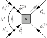
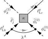
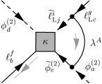
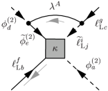
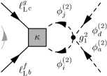
Figure 2: Figures (a)–(d) are the contributions from the gauginos $\lambda^{A}$ to the renormalization of the dimension 5 operator in the MSSM. Figures (e) and (f) show the $D$-term contributions. The gray arrow indicates the fermion flow as defined in [7].

4 Beta-Functions in the Effective Theories

4.1 Standard Model with Additional Majorana Neutrinos

Using the counterterms calculated in the previous section, we find in the SM the following $\beta$-functions $\accentset{(n)}{\beta}_{\kappa}=\mu\frac{\mathrm{d}}{\mathrm{d}\mu}\accentset{(n)}{\kappa}_{gf}$ for the effective vertex below the $n$th threshold:

$$16\pi^{2}\accentset{(n)}{\beta}_{\kappa} = -\frac{3}{2}(Y_{e}^{\dagger}Y_{e})^{T}\>\accentset{(n)}{\kappa}-\frac{3}{2}\,\accentset{(n)}{\kappa}\,(Y_{e}^{\dagger}Y_{e})+\frac{1}{2}\raise 3.0pt\hbox{$\displaystyle\bigl{(}$}\accentset{(n)}{Y}^{\dagger}_{\nu}\accentset{(n)}{Y}_{\nu}\raise 3.0pt\hbox{$\displaystyle\bigr{)}$}^{T}\,\accentset{(n)}{\kappa}+\frac{1}{2}\,\accentset{(n)}{\kappa}\>\raise 3.0pt\hbox{$\displaystyle\bigl{(}$}\accentset{(n)}{Y}^{\dagger}_{\nu}\accentset{(n)}{Y}_{\nu}\raise 3.0pt\hbox{$\displaystyle\bigr{)}$}$$ (14)

$${}+2\,\operatorname{Tr}(Y_{e}^{\dagger}Y_{e})\,\accentset{(n)}{\kappa}+2\,\operatorname{Tr}\raise 3.0pt\hbox{$\displaystyle\bigl{(}$}\accentset{(n)}{Y}^{\dagger}_{\nu}\accentset{(n)}{Y}_{\nu}\raise 3.0pt\hbox{$\displaystyle\bigr{)}$}\,\accentset{(n)}{\kappa}+6\,\operatorname{Tr}(Y_{u}^{\dagger}Y_{u})\,\accentset{(n)}{\kappa}$$

$${}+6\,\operatorname{Tr}(Y_{d}^{\dagger}Y_{d})\,\accentset{(n)}{\kappa}-3g_{2}^{2}\>\accentset{(n)}{\kappa}+\lambda\accentset{(n)}{\kappa}\;.$$

The method used to calculate $\beta$-functions from counterterms in MS-like renormalization schemes for tensorial quantities is described in [4]. For the Yukawa matrix, the $\beta$-function $\accentset{(n)}{\beta}_{Y_{\nu}}$ $(n>1)$ is given by

$$16\pi^{2}\accentset{(n)}{\beta}_{Y_{\nu}} = \accentset{(n)}{Y}_{\nu}\left[\frac{3}{2}\raise 3.0pt\hbox{$\displaystyle\bigl{(}$}\accentset{(n)}{Y}^{\dagger}_{\nu}\accentset{(n)}{Y}_{\nu}\raise 3.0pt\hbox{$\displaystyle\bigr{)}$}-\frac{3}{2}(Y_{e}^{\dagger}Y_{e})+\operatorname{Tr}\raise 3.0pt\hbox{$\displaystyle\bigl{(}$}\accentset{(n)}{Y}^{\dagger}_{\nu}\accentset{(n)}{Y}_{\nu}\raise 3.0pt\hbox{$\displaystyle\bigr{)}$}+\operatorname{Tr}(Y_{e}^{\dagger}Y_{e})\right.$$ (15)

$$\hphantom{\accentset{(n)}{Y}_{\nu}\left[\right.}\left.{}+3\,\operatorname{Tr}(Y_{u}^{\dagger}Y_{u})+3\,\operatorname{Tr}(Y_{d}^{\dagger}Y_{d})-\frac{3}{4}g_{1}^{2}-\frac{9}{4}g_{2}^{2}\right]\;.$$

Calculating the $\beta$-function for the Majorana mass matrix of the singlets yields

$$16\pi^{2}\accentset{(n)}{\beta}_{M} = \raise 3.0pt\hbox{$\displaystyle\bigl{(}$}\accentset{(n)}{Y}_{\nu}\accentset{(n)}{Y}^{\dagger}_{\nu}\raise 3.0pt\hbox{$\displaystyle\bigr{)}$}\,\accentset{(n)}{M}+\accentset{(n)}{M}\,\raise 3.0pt\hbox{$\displaystyle\bigl{(}$}\accentset{(n)}{Y}_{\nu}\accentset{(n)}{Y}^{\dagger}_{\nu}\raise 3.0pt\hbox{$\displaystyle\bigr{)}$}^{T}\;.$$ (16)

4.2 MSSM with Additional Singlets

In the MSSM with additional chiral superfields including sterile neutrinos, the $\beta$-function for the effective vertex below the $n$th threshold is given by

$$16\pi^{2}\accentset{(n)}{\beta}_{\kappa} = (Y_{e}^{\dagger}Y_{e})^{T}\>\accentset{(n)}{\kappa}+\accentset{(n)}{\kappa}\,(Y_{e}^{\dagger}Y_{e})+\raise 3.0pt\hbox{$\displaystyle\bigl{(}$}\accentset{(n)}{Y}^{\dagger}_{\nu}\accentset{(n)}{Y}_{\nu}\raise 3.0pt\hbox{$\displaystyle\bigr{)}$}^{T}\,\accentset{(n)}{\kappa}+\accentset{(n)}{\kappa}\>\raise 3.0pt\hbox{$\displaystyle\bigl{(}$}\accentset{(n)}{Y}^{\dagger}_{\nu}\accentset{(n)}{Y}_{\nu}\raise 3.0pt\hbox{$\displaystyle\bigr{)}$}$$ (17)

$${}+2\,\operatorname{Tr}\raise 3.0pt\hbox{$\displaystyle\bigl{(}$}\accentset{(n)}{Y}^{\dagger}_{\nu}\accentset{(n)}{Y}_{\nu}\raise 3.0pt\hbox{$\displaystyle\bigr{)}$}\,\accentset{(n)}{\kappa}+6\,\operatorname{Tr}(Y_{u}^{\dagger}Y_{u})\,\accentset{(n)}{\kappa}-2g_{1}^{2}\>\accentset{(n)}{\kappa}-6g_{2}^{2}\>\accentset{(n)}{\kappa}\;.$$

For $\accentset{(n)}{\beta}_{Y_{\nu}}$ we obtain

$$16\pi^{2}\accentset{(n)}{\beta}_{Y_{\nu}} = \accentset{(n)}{Y}_{\nu}\left[3\,\accentset{(n)}{Y}^{\dagger}_{\nu}\accentset{(n)}{Y}_{\nu}+Y_{e}^{\dagger}Y_{e}+\operatorname{Tr}\raise 3.0pt\hbox{$\displaystyle\bigl{(}$}\accentset{(n)}{Y}^{\dagger}_{\nu}\accentset{(n)}{Y}_{\nu}\raise 3.0pt\hbox{$\displaystyle\bigr{)}$}+3\operatorname{Tr}(Y_{u}^{\dagger}Y_{u})-g_{1}^{2}-3g_{2}^{2}\right]$$ (18)

and the $\beta$-function for the Majorana mass matrix of the singlets is

$$16\pi^{2}\accentset{(n)}{\beta}_{M} = 2\,\raise 3.0pt\hbox{$\displaystyle\bigl{(}$}\accentset{(n)}{Y}_{\nu}\accentset{(n)}{Y}^{\dagger}_{\nu}\raise 3.0pt\hbox{$\displaystyle\bigr{)}$}\,\accentset{(n)}{M}+2\,\accentset{(n)}{M}\,\raise 3.0pt\hbox{$\displaystyle\bigl{(}$}\accentset{(n)}{Y}_{\nu}\accentset{(n)}{Y}^{\dagger}_{\nu}\raise 3.0pt\hbox{$\displaystyle\bigr{)}$}^{T}\;.$$ (19)

The $\beta$-functions for the gauge couplings and for the Yukawa couplings of the quarks and charged leptons are not listed here. We found them to be the same as in the extended SM or MSSM [8], if one substitutes $Y_{\nu}\rightarrow\accentset{(n)}{Y}_{\nu}$.

4.3 Calculation of the Low-Energy Effective Neutrino Mass Matrix

From the above $\beta$-functions, the low-energy effective neutrino mass matrix can now be calculated as follows: At the GUT scale, we start with the Yukawa matrices $Y_{\nu}$ and the Majorana mass matrix $M$ for the sterile neutrinos. Using the relevant RGE’s (15), (16) or (18), (19) (with the superscripts $(n)$ omitted) together with those of the gauge and the other Yukawa couplings, we calculate the renormalization group running of $Y_{\nu}$, $M$ and the remaining parameters of the theory.

At the first mass threshold, i.e. the largest eigenvalue $M_{n_{G}}$ of $M$, we integrate out the heaviest sterile neutrino and perform tree-level matching according to equation (8). Note that this procedure is only possible in the mass eigenstate basis at the threshold, which is different from the original one at the GUT scale, since the RG evolution produces non-zero off-diagonal entries in $M$. Therefore, the mass matrix has to be diagonalized by a unitary transformation, $M\to U^{T}M\,U$, which leads to the redefinitions $N_{\mathrm{R}}\to U^{T}N_{\mathrm{R}}$, ${}^{\mathrm{C}}\to U^{T}{}^{\mathrm{C}}$ and $Y_{\nu}\to U^{T}Y_{\nu}$ of the singlet neutrino fields and their Yukawa matrix.

Integrating out the heaviest neutrino state yields an effective theory valid at mass scales below $M_{n_{G}}$. The effective dimension 5 operator $\accentset{(n_{G})}{\kappa}$ that gives Majorana masses to the left-handed SM neutrinos appears in this effective theory. Next, $\accentset{(n_{G})}{Y_{\nu}}\,$, $\,\accentset{(n_{G})}{\kappa}$, $\accentset{(n_{G})}{M}$, $Y_{e}$ etc. are evolved down to the next threshold, the largest eigenvalue of the remaining mass matrix $\accentset{(n_{G})}{M}$. The RGE’s that determine the running of the dimension 5 effective operator between the thresholds are given by equation (14) or (17), respectively.

Again, changing to the mass eigenstate basis, integrating out the singlet neutrino corresponding to this threshold and performing tree-level matching gives another contribution to the effective dimension 5 operator. The quantities in this effective theory are now evolved down to the next threshold and so on. This procedure finally yields the low-energy effective neutrino mass matrix.

4.4 Running of the Mixing Angle in an Example with Two Generations

Numerical results for the RG evolution of the mixing angle $\theta$ in a generic example with two generations of lepton doublets and two singlets are shown as solid lines in figure 3 for the SM and in figure 4 for the MSSM. Here, $\theta$ is defined as the angle that appears in the leptonic mixing matrix $V=U_{e}^{\dagger}U_{\nu}$, where $U_{e}$ diagonalizes $Y_{e}^{\dagger}Y_{e}$ and $U_{\nu}$ diagonalizes the effective mass matrix of the active (non-sterile) neutrinos. Below the lowest threshold, the latter is proportional to the coupling $\kappa$. In the energy region where heavy neutrinos are present, the effective Majorana mass matrix of the non-sterile neutrinos is given by $\accentset{(n)}{\kappa}+2\accentset{(n)}{Y}_{\nu}^{T}\accentset{(n)}{M}^{-1}\accentset{(n)}{Y}_{\nu}$.

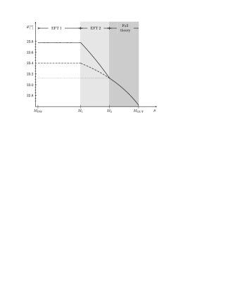
Figure 3: RG evolution of the mixing angle $\theta$ in the extended SM with 2 generations of lepton doublets and 2 singlets. We used $M_{\mathrm{GUT}}=10^{16}$ GeV and the initial conditions $M_{1}(M_{\mathrm{GUT}})=10^{8}$ GeV, $M_{2}(M_{\mathrm{GUT}})=10^{12}$ GeV for the Majorana masses of the heavy neutrinos at this scale. Besides, we chose the initial values of the Yukawa coupling matrices $Y_{\nu}(M_{\mathrm{GUT}})$ to be real with (untuned) entries between $0.025$ and $1$. Further explanations are given in the text.

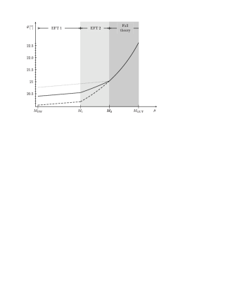
Figure 4: RG evolution of the mixing angle $\theta$ in the extended MSSM with 2 generations of lepton doublets, 2 singlets and $\braket{\phi^{(2)}}/\braket{\phi^{(1)}}=:\tan\beta=35$ as well as $M_{\mathrm{SUSY}}\approx M_{\mathrm{EW}}$ for simplicity. (A moderate change of the SUSY breaking scale $M_{\mathrm{SUSY}}$ does not change the qualitative picture.) The other parameters are the same as in the SM case (cf. figure 3).

The transitions to the various effective theories at the mass thresholds lead to pronounced kinks in the evolution. For comparison, the dotted and dashed lines in figures 3 and 4 show the results when both heavy neutrinos are integrated out at the higher or the lower threshold, respectively. Obviously, this produces large deviations from the true evolution, and the correct result need not even lie between the two extreme cases. Although this is only shown for the SM in our example, the same happens in the MSSM, if suitable initial values for the Yukawa couplings are chosen. Consequently, the correct running of the mixing angle cannot be reproduced by integrating out all heavy neutrinos at some intermediate mass scale $M_{\mathrm{int}}\in[M_{1},M_{2}]$ in general.

5 Discussion and Conclusions

We have calculated the RGE’s for the evolution of a see-saw neutrino mass matrix from the GUT scale to the electroweak scale in an extension of the SM and the MSSM by an arbitrary number of gauge singlets with Majorana masses. These masses need not be degenerate and can even have a large hierarchy, as pointed out in the introduction. At each mass threshold, the corresponding sterile fermion is integrated out, which leads to an effective intermediate theory and affects the RG evolution of the neutrino masses, mixing angles and CP phases. To obtain the low-energy neutrino mass matrix from the Yukawa and Majorana mass matrices given at the GUT scale, the RGE’s for the various effective theories have to be solved. In a numerical analysis for two flavours and two singlets, we have found that the renormalization group evolution of the mixing angle in the case where the heavy degrees of freedom are integrated out appropriately differs substantially from that in the case where all of them are integrated out at a common scale. The correct running can in general not even be reproduced by integrating out all heavy neutrinos at some intermediate mass scale. Obviously, similar effects exist for the RG evolution of all parameters of a given theory, such as mass eigenvalues, mixings and CP phases.

References

- [1] For an introduction see for example E. K. Akhmedov, Neutrino physics (2000), hep-ph/0001264.
- [2] P. H. Chankowski and Z. Pluciennik, Renormalization group equations for seesaw neutrino masses, Phys. Lett. B316 (1993), 312 (hep-ph/9306333).
- [3] K. S. Babu, C. N. Leung and J. Pantaleone, Renormalization of the neutrino mass operator, Phys. Lett. B319 (1993), 191 (hep-ph/9309223).
- [4] S. Antusch, M. Drees, J. Kersten, M. Lindner and M. Ratz, Neutrino mass operator renormalization revisited, Phys. Lett. B519 (2001), 238–242 (hep-ph/0108005).
- [5] S. Antusch, M. Drees, J. Kersten, M. Lindner and M. Ratz, Neutrino mass operator renormalization in two Higgs doublet models and the MSSM, Phys. Lett. B525 (2002), 130 (hep-ph/0110366).
- [6] S. Antusch and M. Ratz, Supergraph Techniques and Two-Loop Beta-Functions for Renormalizable and Non-Renormalizable Operators, hep-ph/0203027.
- [7] A. Denner, H. Eck, O. Hahn and J. Küblbeck, Feynman rules for fermion number violating interactions, Nucl. Phys. B387 (1992), 467.
- [8] See for example P. H. Chankowski and S. Pokorski, Quantum corrections to neutrino masses and mixing angles, Int. J. Mod. Phys. A17 (2002), 575–614 (hep-ph/0110249)