Department of Mathematical Physics and Astronomy, University of Ghent, Krijgslaan 281 (S9), 9000 Ghent, Belgium.

Abstract.We propose an alternative perturbative expansion for QCD. All scheme and scale dependence is reduced to one free parameter. Fixing this parameter with a fastest apparent convergence criterion gives sensible results in the whole energy region. We apply the expansion to the calculation of the zero flavor triple gluon vertex, the quark gluon vertex, the gluon propagator and the ghost propagator. A qualitative agreement with the corresponding lattice results is found.

1 Introduction

Perturbation theory is by far the most successful tool to get quantitative predictions from a field theory. Unfortunately, the results depend on the renormalization scale and scheme and the number of free parameters describing this dependence grows with the order of truncation. In most cases one does not bother too much about this dependence and simply chooses a scheme ($\overline{MS}$, MOM,$\ldots$) which is supposed to give good results. More sophisticated approaches select a different ideal scheme for each perturbative series. Most cited in this context are Stevenson’s principle of minimal sensitivity [1] and Grunberg’s method of effective charges [2].

In this paper we will reorganize the conventional perturbation series in a new alternative expansion, which has only one redundant free parameter, the expansion parameter itself. This parameter will be fixed by a fastest apparent convergence criterion (facc). We find similar results as for the ordinary QCD perturbation theory in the UV-region and for intermediate energies. In the IR-region on the contrary, our expansion still gives sensible results whereas the normal perturbation theory becomes useless if one approaches the Landau-pole.

In section 2 we will first review some of the major aspects of the ordinary perturbation theory and then use this as starting point for the alternative expansion. Some results will be presented in section 3. We perform calculations on the triple gluon vertex, the quark gluon vertex, the gluon propagator and the ghost propagator. Our results are compared with the conventional perturbation theory and with the corresponding lattice results. We also show that the reason for the IR finite results lies in a peculiar behavior of the running expansion parameter $y$, resulting from the facc. This behavior should be contrasted with the running coupling $\alpha$ that Shirkov and Solovtsov obtain by imposing analyticity [3]. While we find a universal power behavior for $y$, they find an IR-finite value for $\alpha$ at zero momentum.

2 Rewriting perturbation theory

In the following we will consider the perturbative calculation of a renormalization scheme and scale invariant quantity $\mathcal{R}$, that is function of only one external scale $q^{2}$, in a massless version of QCD . In ordinary perturbation theory one finds a row of approximations $\mathcal{R}^{n}$ for $\mathcal{R}$, with

$$\mathcal{R}^{n}={h^{(n)}}^{N}(1+r_{1}(q^{2})h^{(n)}+r_{2}(q^{2}){h^{(n)}}^{2}+\ldots+r_{n}(q^{2}){h^{(n)}}^{n})~{}.$$ (2.1)

With $N$ depending on the calculated quantity. The coupling constant $h^{(n)}$ is the solution of

$$\beta_{0}\ln\frac{\mu^{2}}{\Lambda^{2}} = \frac{1}{h}+\frac{\beta_{1}}{\beta_{0}}\ln(\beta_{0}h)+$$ (2.2)

$$\int^{h}_{0}\!\!\!dx\left(\frac{1}{x^{2}}-\frac{\beta_{1}}{\beta_{0}}\frac{1}{x}-\frac{\beta_{0}}{\beta_{0}x^{2}+\beta_{1}x^{3}+\ldots+\beta_{n}x^{n+2}}\right),~{}~{}~{}$$

with $\mu^{2}\frac{\partial}{\partial\mu^{2}}h\equiv-(\beta_{0}h^{2}+\beta_{1}h^{3}+\beta_{2}h^{4}+\ldots).$ As mentioned in the introduction, every truncation $\mathcal{R}^{n}$ is highly scale and scheme dependent. One can for instance describe this dependence with the free parameters [1] $\beta_{0}\ln\frac{\mu^{2}}{\Lambda^{2}},\beta_{2},\beta_{3},\ldots,\beta_{n}.$ The dependence of the coefficients $r_{i}$ on each of these parameters, cancels the dependence of the coupling constant $h^{(n)}$ up to order ${h^{(n)}}^{n+1}$.

In many cases one simply chooses a scheme ($\overline{MS}$, MOM, $\ldots$) and sets the scale $\mu^{2}$ equal to the external scale $q^{2}$. To get reliable results, one must hope that the first, second, or third order approximation lies close enough to the exact result. The working hypothesis of perturbation theory is that the perturbation series is asymptotic to the exact result $\mathcal{R}$ [4]. One then obtains an error estimation, by assuming that

$$\left|\frac{\mathcal{R}-\mathcal{R}^{n}}{\mathcal{R}}\right|\sim\left|\frac{\mathcal{R}^{n+1}-\mathcal{R}^{n}}{\mathcal{R}^{n+1}}\right|\equiv\Delta^{n}~{}~{}.$$ (2.3)

Other approaches fix the scale/scheme by imposing a condition on the truncated series. The minimal sensitivity condition [1] gives a different scale/scheme for every approximation. The method of the effective charges [2], sets $q^{2}=\mu^{2}$, the free parameters are then obtained by demanding the coefficients $r_{i}$ to be zero. One now also finds $\Delta^{n}$ to give a good estimation of the error [5].

As a consequence of asymptotic freedom, conventional perturbation theory works well in the UV-region, which is reflected in low values of $\Delta^{n}$ (n=1,2,3) for high values of $q^{2}$. Unfortunately $\Delta^{n}$ gets larger if we lower the external scale $q^{2}$. This signals that one has to add non-perturbative power corrections to the conventional perturbation theory [4]. For intermediate energies, the sum rules [6] successfully relate many of these power corrections to a few condensates. A further lowering of $q^{2}$ towards the IR-region is catastrophic in most cases , $\Delta^{n}$ diverges together with ${\mathcal{R}}^{n}$ as one encounters the Landau-pole and perturbation theory becomes useless.

The alternative expansion we propose in this paper has no Landau-pole problem and gives sensible results up to $q^{2}=0$ with a reasonable error estimation. We simply have to exchange $h$ for a new expansion parameter $y$, defined by

$$\beta_{0}\ln\frac{\mu^{2}}{\Lambda^{2}}\equiv\frac{1}{y}+\frac{\beta_{1}}{\beta_{0}}\ln(\beta_{0}y).$$ (2.4)

From (2.1),(2.2) and (2.4) we find after some calculations

$$\mathcal{R} = y^{N}\Bigg{(}1+y\bigg{[}A_{1}+Nk\bigg{]}+y^{2}\bigg{[}A_{2}+N\Big{(}\frac{\beta_{2}}{\beta_{0}}-(\frac{\beta_{1}}{\beta_{0}})^{2}\Big{)}$$

$$+k\Big{(}(N+1)A_{1}+N\frac{\beta_{1}}{\beta_{0}}\Big{)}+k^{2}\frac{N}{2}(N+1)\bigg{]}$$

$$+y^{3}\bigg{[}A_{3}+A_{1}(N+1)\Big{(}\frac{\beta_{2}}{\beta_{0}}-(\frac{\beta_{1}}{\beta_{0}})^{2}\Big{)}+\frac{N}{2}\Big{(}\frac{\beta_{3}}{\beta_{0}}-(\frac{\beta_{1}}{\beta_{0}})^{3}\Big{)}$$

$$+k\Big{(}A_{1}(N+1)\frac{\beta_{1}}{\beta_{0}}+(N+2)A_{2}+N(N+2)\frac{\beta_{2}}{\beta_{0}}$$

$$-N(N+1)(\frac{\beta_{1}}{\beta_{0}})^{2}\Big{)}$$

$$+k^{2}\Big{(}\frac{A_{1}}{2}(N+2)(N+1)+N(N+\frac{3}{2})\frac{\beta_{1}}{\beta_{0}}\Big{)}$$

$$+k^{3}\Big{(}\frac{N}{6}(N+2)(N+1)\Big{)}\bigg{]}+\ldots\Bigg{)}$$

with

$$k \equiv k(q^{2},y)=\frac{1}{y}+\frac{\beta_{1}}{\beta_{0}}\ln(\beta_{0}y)-\beta_{0}\ln\frac{q^{2}}{{\Lambda_{\overline{MS}}}^{2}}$$ (2.6)

$$A_{i} \equiv r_{i}(\mu^{2}=q^{2},\overline{MS})$$ (2.7)

The $\beta$-coefficients $\beta_{2},\beta_{3},\ldots$ are also in the $\overline{MS}$-scheme.

We now find a row of approximations $\mathcal{R}^{n}(y)$ with all the redundant dependence residing in one single free parameter $\beta_{0}\ln\frac{\mu^{2}}{\Lambda^{2}}$ or equivalently $y$. All the other scheme dependence has disappeared, because it was eliminated from the expansion parameter. This might seem strange, since we explicitly refer to the $\overline{MS}$ scheme, but one can show that another choice for the reference scheme changes the coefficients $A_{i}$ and $\beta_{i}$ in such a way that it exactly compensates the shift of $k~{}(k\rightarrow k^{\prime}=k+2\beta_{0}\ln\frac{\Lambda^{\prime}}{\Lambda_{\overline{MS}}})$.

To fix the expansion parameter $y$ for each value of $q^{2}$, we will have to impose some condition. We choose a facc: for each approximation $\mathcal{R}^{n}(y)$ we will set $y$ equal to $y_{n}$, the expansion parameter that minimizes the relative correction to the first order truncation of the series:

$$\min\left|\frac{\mathcal{R}^{n}(y)-\mathcal{R}^{1}(y)}{\mathcal{R}^{1}(y)}\right|=\left|\frac{\mathcal{R}^{n}(y_{n})-\mathcal{R}^{1}(y_{n})}{\mathcal{R}^{1}(y_{n})}\right|$$ (2.8)

We will use the same error estimation as for the conventional perturbation theory:

$$\Delta^{n}\equiv\left|\frac{\mathcal{R}^{n+1}(y_{n+1})-\mathcal{R}^{n}(y_{n})}{\mathcal{R}^{n+1}(y_{n+1})}\right|$$ (2.9)

(Notice the difference: the fixing of y is done on the series, while the error is estimated on the results obtained after fixing.) As for any other possible fixing condition (e.g. minimal sensitivity, another facc,…), there is no rigorous mathematical motivation for the condition we use. The true motivation lies in the fact that it generates sensible results with a good error estimation. This is the case for all the calculations we have performed so far. If we use, for example, the more obvious facc, where one minimizes the relative correction to the zero order truncation $y^{N}$, we do not find sensible results for the whole range of energies. There is a discontinuity at the point that separates the high energy region where this correction minimizes to zero, and the low energy region where it minimizes to a nonzero value. Let us now present some results obtained from (2) and (2.8).

3 Some results

We now demonstrate the $y$-expansion on some quantities that also have been calculated on the lattice. All the needed two and three loop results have been calculated by Chetyrkin and Retey [8]. Everything is in Landau gauge for $N_{c}=3$ and $N_{f}=0$. We will take the method of effective charges to be exemplary for the ordinary perturbation theory, but similar results are found with any other approach to the conventional perturbation theory.

3.1 Triple gluon vertex

There are several ways in which one can associate a (renormalization) scale and scheme invariant coupling constant with the triple gluon 3-point function

$$G^{(3)abc}_{\mu\upsilon\rho}(p,q)\equiv i^{2}\int\!\!\!dxdye^{-i(px+qy)}<T[A_{\mu}^{a}(x)A_{\upsilon}^{b}(y)A_{\rho}^{c}(0)]>,$$ (3.10)

or more precisely with its related vertex function $\Gamma_{\mu\upsilon\rho}^{abc}(p,q,-p-q)$, defined by

$$G^{(3)abc}_{\mu\upsilon\rho}(p,q)\equiv D_{\mu\mu^{\prime}}^{ad}(-p)D_{\upsilon\upsilon^{\prime}}^{be}(-q)D_{\rho\rho^{\prime}}^{cf}(-p-q)\Gamma_{\mu^{\prime}\upsilon^{\prime}\rho^{\prime}}^{def}(p,q,-p-q),$$ (3.11)

where

$$D_{\mu\upsilon}^{ab}(q)\equiv i\int\!\!\!dxe^{iqx}<T[A_{\mu}^{a}(x)A_{\upsilon}^{b}(0)]>.$$ (3.12)

If one sets one external momentum to zero, one finds [8] that the vertex-function can be written as:

$$\Gamma_{\mu\upsilon\rho}^{abc}(q,-q,0)=-igf^{abc}\Big{(}(2g_{\mu\upsilon}q_{\rho}-g_{\mu\rho}q_{\upsilon}-g_{\rho\upsilon}q_{\mu})T_{1}(q^{2})\Big{)}$$

$$-(g_{\mu\upsilon}-\frac{q_{\mu}q_{\upsilon}}{q^{2}})q_{\rho}T_{2}(q^{2})\Big{)}$$ (3.13)

The coupling that was calculated on the lattice [9, 10] is found to be ([8],section 6.4):

$$\alpha_{s}(q^{2})\equiv 4\pi h^{\widetilde{{\textrm{{MOM}}}}\textrm{gg}}(q^{2})=h\Big{(}T_{1}(-q^{2})-\frac{1}{2}T_{2}(-q^{2})\Big{)}^{2}Z(-q^{2})^{3},$$ (3.14)

$$\textrm{where}\qquad\qquad h = \frac{g^{2}}{16\pi^{2}},$$ (3.15)

$$D_{\mu\upsilon}^{ab}(q) = \delta^{ab}(g_{\mu\upsilon}-\frac{q_{\mu}q_{\upsilon}}{q^{2}})\frac{Z(q^{2})}{q^{2}}.$$ (3.16)

One can easily check the scheme and scale independence of $\alpha_{s}$. The three-loop result for $h^{\widetilde{\textrm{MOM}}\textrm{gg}}$ in the $\overline{MS}$-scheme for $\mu^{2}=q^{2}$ is,[8]:

$$h^{\widetilde{\textrm{MOM}}\textrm{gg}} = h+h^{2}[\frac{70}{3}]+h^{3}[\frac{516217}{576}-\frac{153}{4}\zeta_{3}]+$$ (3.17)

$$h^{4}[\frac{304676635}{6912}-\frac{299961}{64}\zeta_{3}-\frac{81825}{64}\zeta_{5}],$$

where $\zeta_{i}$ is the Riemann zeta function. From this we can read of the coefficients $A_{1},A_{2},A_{3}$ that are needed in (2). The $\beta$-coefficients in the $\overline{MS}$-scheme have been calculated up to four loops in [11]:

$$\beta_{0}=11,\qquad\beta_{1}=102,\qquad\beta_{2}=\frac{2857}{2},\qquad\beta_{3}=\frac{149753}{6}+3564\zeta_{3}.$$ (3.18)

We will compare our two and three loop results for $\alpha_{s}(q^{2})$ obtained from (2) (with $N=1$) and (2.8) with the results obtained from the method of effective charges [2] or equivalently in the $\widetilde{\textrm{MOM}}$gg-scheme defined on the triple gluon vertex. The two and three loop $\widetilde{\textrm{MOM}}$-scheme results are found as the solution of (2.2) with $n=2,3$. The $\widetilde{\textrm{MOM}}$-scheme $\beta$-coefficients can be easily obtained from (3.17) and (3.18):

$$\beta_{2}^{\widetilde{\textrm{MOM}\textrm{gg}}} = \frac{186747}{64}-\frac{1683}{4}\zeta_{3},$$

$$\beta_{3}^{\widetilde{\textrm{MOM}\textrm{gg}}} = \frac{20783939}{128}-\frac{1300563}{32}\zeta_{3}-\frac{900075}{32}\zeta_{5}.$$ (3.19)

While the $\Lambda$ parameter is given by [12]:

$$2\beta_{0}\ln\frac{\Lambda_{\widetilde{\textrm{MOM}\textrm{gg}}}}{\Lambda_{\overline{MS}}}=\frac{70}{3}.$$ (3.20)

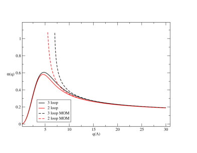
Our two and three loop results are plotted together with the two and three loop $\widetilde{\textrm{MOM}}$-results in figs. 2 and 2.

Figure 1: $\alpha_{s}(q)$ ($q$ in units of $\Lambda_{\overline{\textrm{MS}}})$, for 2 and 3 loops in the $y$-expansion and in the $\widetilde{\textrm{MOM}}$-scheme.

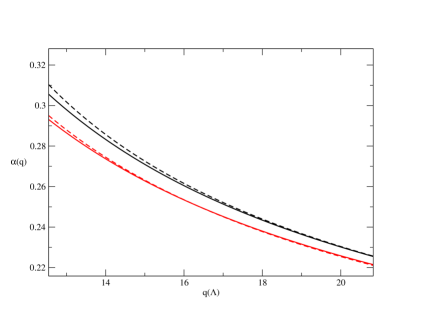
Figure 2: Zooming in on the intermediate energy region of fig. 2

We can clearly distinct three regions. For $q>30\Lambda_{\overline{\textrm{MS}}}$ one finds the UV-region: the four results for $\alpha_{s}$ coincide and the perturbation theory is completely reliable. The intermediate energies region goes from $q\approx 30\Lambda_{\overline{\textrm{MS}}}$ down to $q\approx 10\Lambda_{\overline{\textrm{MS}}}$. A difference grows between the two and three loop results, but for both orders the $y$-expansion results still coincide with the $\widetilde{\textrm{MOM}}$ results. Power corrections are expected. For $q<10\Lambda_{\overline{\textrm{MS}}}$ we find ourselves in the IR-region. The $\widetilde{\textrm{MOM}}$ results diverge while the $y$-expansion results continue to behave in a sensible way.

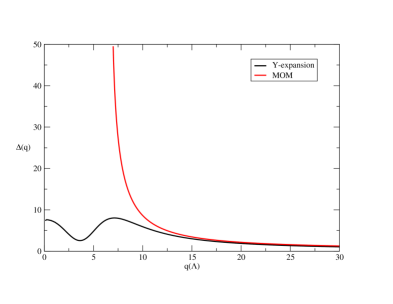
Figure 3: $q$ (in units of $\Lambda_{\overline{\textrm{MS}}})\rightarrow\Delta^{2}=\left|\frac{\alpha_{s}^{(2)}-\alpha_{s}^{(3)}}{\alpha_{s}^{(3)}}\right|$ (in $\%$), for both the $y$-expansion and the $\widetilde{\textrm{MOM}}$ scheme.

The same conclusions can be read from fig. 3, where $\Delta^{2}$ (see (2.3)) is plotted, both for the $\widetilde{\textrm{MOM}}$ scheme and for the $y$-expansion. In the IR-region the error estimation diverges for the $\widetilde{\textrm{MOM}}$ scheme, while it stays in an acceptable interval for the $y$-expansion.

It is the facc (2.8) that keeps the error estimation under control in the IR. This criterion, and in fact every other sensible criterion, will select for each momentum $q$ a value for y that makes the higher order ($n>1$) terms in the series (2) as small as possible. Both for small values of $q$ ($q\ll\Lambda_{\overline{\textrm{MS}}}$) and for large values ($q\gg\Lambda_{\overline{\textrm{MS}}}$) it is the value of

$$yk(q^{2},y)=1+y\frac{\beta_{1}}{\beta_{0}}\ln(\beta_{0}y)-y\beta_{0}\ln\frac{q^{2}}{{\Lambda_{\overline{MS}}}^{2}},$$ (3.21)

that determines the size of these higher order terms. For $q\gg\Lambda_{\overline{\textrm{MS}}}$ the large logarithm will be compensated by the $y$ that multiplies it. One finds the usual high energy running of the expansion parameter:

$$y\stackrel{{\scriptstyle q\rightarrow\infty}}{{=}}\frac{1}{\beta_{0}\ln\frac{q^{2}}{\Lambda_{\overline{MS}}^{2}}+c}~{}~{}~{},$$ (3.22)

with $c$ a constant. This gives

$$k(q^{2},y)y\stackrel{{\scriptstyle q\rightarrow\infty}}{{\approx}}\frac{1}{\beta_{0}\ln\frac{q^{2}}{\Lambda_{\overline{MS}}^{2}}}\left(c-\frac{\beta_{1}}{\beta_{0}}\ln(\ln\frac{q^{2}}{\Lambda_{\overline{MS}}^{2}})\right).$$ (3.23)

For $q\ll\Lambda_{\overline{\textrm{MS}}}$ the same cancellation can not occur since $y$ must be positive, the large logarithm will now be compensated by the logarithm in the second term, we find a power behavior for $y$:

$$y\stackrel{{\scriptstyle q\rightarrow 0}}{{=}}c^{\prime}\left(\frac{q^{2}}{\Lambda_{\overline{MS}}^{2}}\right)^{\frac{\beta_{0}^{2}}{\beta_{1}}}$$ (3.24)

and

$$k(q^{2},y)y\stackrel{{\scriptstyle q\rightarrow 0}}{{\approx}}1.$$ (3.25)

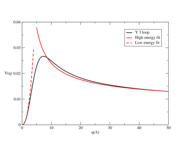
This high and low energy behavior of the expansion parameter $y$ is completely universal, it is independent of the order of truncation, of the coefficients $A_{i}$ and to a certain extent of the criterion that was used. The running of $y$ is depicted in fig. 4 together with the fitted low (3.24) and high (3.22) energy behavior for the three loop truncation.

Figure 4: $y(q)$ ($q$ in units of $\Lambda_{\overline{\textrm{MS}}}$) for the tree loop truncation. Also depicted: the low and high energy fits (3.24) and (3.22).

If one would use the series itself to estimate the truncation error, (3.25) would seem to invalidate the expansion for low energies, since the higher order terms become order 1. However, if you look at the the row of truncations (2.9) to estimate the error , the expansion remains valid (at least for low orders) since $2.5\%<\Delta^{2}<7.5\%$ (see fig. 2.3). We have found a same behavior of $\Delta^{2}$ for every other possible vertex-coupling that could be calculated from [8].

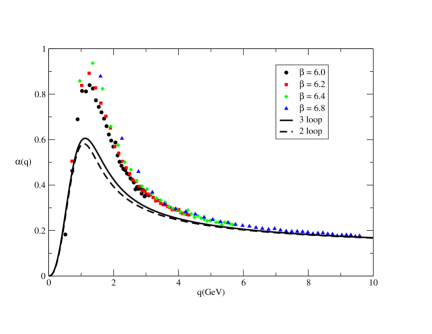
Figure 5: The lattice results [9] for the coupling from the triple gluon vertex with the two and three loop results of the y-expansion for $\Lambda_{\overline{MS}}$=237 Mev.

We will finally compare our results with the lattice results of [9]. This requires a fit of $\Lambda_{\overline{MS}}$, which was done for the two and three loop $\widetilde{\textrm{MOM}}$ results in [9] and [8] in the intermediate energy region (3 Gev-10 Gev). It was found that the $\widetilde{\textrm{MOM}}$-results could be best fitted to the lattice results if a power correction $\frac{c}{p^{2}}$ was added. The fitted two and three loop values of $\Lambda_{\overline{MS}}$ are: 235 Mev and 238 Mev. The three loop power correction is 30$\%$ less then the two loop one.

Since in the intermediate energy region the results of the $y$-expansion are the same as the $\widetilde{\textrm{MOM}}$ results we can rely on the aforementioned fits. We will use the same value $\Lambda_{\overline{MS}}$=237 Mev, for every order. The two and three loop results of the $y$-expansion are plotted together with the lattice results in fig. 5. As expected, the difference between our results and the lattice result can be fitted as a power correction for $q>3$ Gev. The amplitude of our maximum is significantly smaller then the amplitude for the lattice maximum in the IR region. But both maxima seem to approach each other, our amplitude grows larger with the order of truncation while the lattice amplitude becomes smaller for larger volumes (smaller $\beta$).

3.2 The quark gluon vertex

Again, there are several ways one can associate a scale and scheme invariant running coupling with the (zero flavor) quark-gluon vertex $\Lambda_{\mu ij}^{a}$, which is defined by:

$$G_{\mu ij}^{(3)a}(p,q)=S_{ii^{\prime}}(-p)\Lambda_{\mu^{\prime}i^{\prime}j^{\prime}}^{d}(p,q,-q-p)S_{j^{\prime}j}(q)D_{\mu^{\prime}\mu}^{ad}(p+q)~{}~{}~{},$$ (3.26)

where $G_{\mu ij}^{(3)a}$ is the corresponding 3-point function and $S_{ij}$ is the quark propagator. After setting the external gluon momentum equal to zero, the vertex can be written as, [8]:

$$\Lambda_{\mu ij}^{a}(-q,q,0)=gT_{ij}^{a}\left[\gamma_{\mu}\Lambda_{g}(q^{2})+\gamma_{\upsilon}\left(g_{\mu\upsilon}-\frac{q_{\mu}q_{\upsilon}}{q^{2}}\right)\Lambda_{g}^{T}(q^{2})\right]$$ (3.27)

We find the coupling constant that was defined and calculated on the lattice in [13, 14] to be:

$$g(q^{2})=4\pi h^{\frac{1}{2}}\left(\Lambda_{g}(-q^{2})+\Lambda_{g}^{T}(-q^{2})\right)Z^{\frac{1}{2}}(-q^{2})Z_{2}(-q^{2})~{}~{},$$ (3.28)

where

$$S_{ij}(q)=-\delta_{ij}\frac{q\!\!\!/}{q^{2}}Z_{2}(-q^{2}).$$ (3.29)

From [8] one finds, with $\mu^{2}=q^{2}$ in the $\overline{\textrm{MS}}$ scheme:

$$g(q^{2}) = 4\pi h^{\frac{1}{2}}\Big{(}1+h[\frac{151}{24}]+h^{2}[\frac{87557}{384}-47\zeta_{3}]+$$ (3.30)

$$h^{3}[\frac{266866067}{27648}-\frac{824999}{288}\zeta_{3}-\frac{349225}{1152}\zeta_{5}]+\ldots\Big{)}$$

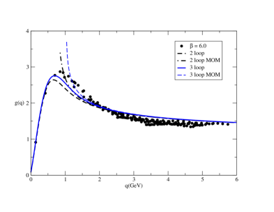
Putting these coefficients, together with the $\beta$-coefficients (3.18) in (2) (now for $N$=1/2) and fixing $y$ with the facc (2.8) will give us the two and three loop $y$-expansion results for $g(q^{2})$.

The two and three loop $\widetilde{\textrm{MOM}}$ scheme results can now be found as $4\pi(h^{(n)})^{\frac{1}{2}}$ (n=2,3), with $h^{(n)}$ solution of (2.2). From (3.18) and (3.30) we can easily determine the needed $\beta$-coefficients:

$$\beta_{2}^{\widetilde{\textrm{MOM}}\textrm{qg}} = \frac{185039}{48}-1034\zeta_{3}~{}~{},$$

$$\beta_{3}^{\widetilde{\textrm{MOM}}\textrm{qg}} = \frac{32456317}{192}-\frac{4134361}{72}\zeta_{3}-\frac{3841475}{288}\zeta_{5}~{}~{}.$$ (3.31)

The $\Lambda$-parameter is now given by:

$$2\beta_{0}\ln\frac{\Lambda_{\widetilde{\textrm{MOM}\textrm{qg}}}}{\Lambda_{\overline{MS}}}=\frac{151}{12}.$$ (3.32)

Figure 6: The lattice results [14] for the coupling from the quark gluon vertex with the two and three loop results from the $y$-expansion and the $\widetilde{\textrm{MOM}}$ scheme, with $\Lambda_{\overline{MS}}$=237 Mev.

The results are completely similar to the results for the triple gluon vertex. Instead of performing a separate fit we simply take the value ($237$ Mev) for $\Lambda_{\overline{MS}}$ obtained from the triple gluon vertex, to compare with the lattice result. From fig. 6 we can again observe a turnover for the $y$-expansion results and the lattice results around 1 Gev, where the $\widetilde{\textrm{MOM}}$ scheme results diverge. We finally note that the lattice results were obtained for a (small) non-zero quark mass, while our results are for a massless quark, so we should not be too enthusiastic about the small amplitude difference in the IR-region.

3.3 The gluon propagator

The $y$-expansion will now be applied to the calculation of the scale and scheme invariant gluon propagator $\widehat{D}_{\mu\upsilon}^{ab}(-q^{2})$ defined by:

$$\widehat{D}_{\mu\upsilon}^{ab}(-q^{2})\equiv f(h)D_{\mu\upsilon}^{ab}(-q^{2}),$$ (3.33)

with

$$\mu^{2}\frac{\partial}{\partial\mu^{2}}D_{\mu\upsilon}^{ab}(-q^{2})\equiv(\gamma_{3_{0}}h+\gamma_{3_{1}}h^{2}+\gamma_{3_{2}}h^{3}+\ldots)D_{\mu\upsilon}^{ab}(-q^{2})$$ (3.34)

and

$$\mu^{2}\frac{\partial}{\partial\mu^{2}}f(h)\equiv-(\gamma_{3_{0}}h+\gamma_{3_{1}}h^{2}+\gamma_{3_{2}}h^{3}+\ldots)f(h).$$ (3.35)

The general solution of (3.35) is:

$$f(h) = \lambda h^{\frac{\gamma_{3_{0}}}{\beta_{0}}}\Big{[}1+\Big{(}\frac{\gamma_{3_{1}}}{\beta_{0}}-\frac{\gamma_{3_{0}}\beta_{1}}{\beta_{0}^{2}}\Big{)}h+\Big{(}\frac{\gamma_{3_{2}}}{2\beta_{0}}-\frac{\gamma_{3_{1}}\beta_{1}}{2\beta_{0}^{2}}+\frac{\gamma_{3_{0}}}{2\beta_{0}}(\frac{\beta_{1}}{\beta_{0}})^{2}-\frac{\gamma_{3_{0}}\beta_{2}}{2\beta_{0}^{2}}$$ (3.36)

$$+\frac{\gamma_{3_{1}}^{2}}{2\beta_{0}^{2}}-\frac{\gamma_{3_{1}}\gamma_{3_{0}}\beta_{1}}{\beta_{0}^{3}}+\frac{\gamma_{3_{0}}^{2}\beta_{1}^{2}}{2\beta_{0}^{4}}\Big{)}h^{2}+\ldots\Big{]},$$

with $\lambda$ a constant that determines the overall wave function renormalization. One can easily check the scale and scheme independence of $\widehat{D}$. From [8] and (3.36) we find for $\widehat{Z}^{-1}(-q^{2})$ (cf. (3.16)), with $\mu^{2}=q^{2}$ and in the $\overline{MS}$ scheme:

$$\widehat{Z}^{-1}(-q^{2})=\lambda^{-1}h^{-\frac{13}{22}}(1+h[-\frac{25085}{2904}]+h^{2}[-\frac{412485993}{1874048}+\frac{9747}{352}\zeta_{3}]+\ldots).$$ (3.37)

(Unfortunately we can only determine ${\widehat{Z}}^{-1}$ up to second order since for the third order result one needs, besides the known third order coefficient for $Z^{-1}$ and the four loop $\beta$-coefficient also the four loop $\gamma_{3}$-coefficient, which is not available at the moment. As a consequence we are not able to perform an error estimation.) The 2 loop $y$-expansion result for ${\widehat{Z}}^{-1}$ is now obtained from (2), (2.8) and (3.37). The 2 loop MOM scheme result is found as $\lambda^{-1}{h^{(2)}}^{-\frac{13}{22}}$ where $h^{(2)}$ is the solution of (2.2) with

$$\beta_{2}^{\textrm{MOMz}}=\frac{105708585}{29744}-\frac{107217}{208}\zeta_{3}\qquad\textrm{and}\qquad\Lambda_{\textrm{MOMz}}=\Lambda_{\overline{MS}}\exp^{\frac{25085}{37752}}.$$ (3.38)

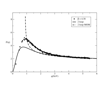
Figure 7: Lattice result [15] for the gluon propagator ($q^{2}\times D(q^{2})$) with the two loop results from the $y$-expansion and the MOM scheme, $\Lambda_{\overline{MS}}$=237Mev.

The 2-loop results for $Z(q^{2})$ (Euclidean momentum) are shown together with a lattice result from [15] in fig. 7. We now had two fit two things: the scale $\Lambda_{\overline{MS}}$ and the relative wave function renormalization $\lambda$. Again, we choose the triple gluon vertex value (237 Mev) for $\Lambda_{\overline{MS}}$. $\lambda$ is simply determined by fitting the tail of the 2-loop results on the tail of the lattice result (at about 5.5 Gev). The overall agreement of our result with the lattice is similar as for the vertices. In the deep IR-region, however, there is a discrepancy: in [15] it is argued, by extrapolation to infinite lattice-volume, that the zero momentum gluon propagator is finite while we find a singular zero momentum propagator. Indeed, from the IR-behavior of $y$ (3.24) and the expansion for ${\widehat{Z}}^{-1}$ (3.37) one easily obtains the IR-behavior of $D(q)$:

$$D(q)\stackrel{{\scriptstyle q\rightarrow 0}}{{\sim}}\frac{y(q)^{\frac{\gamma_{3_{0}}}{\beta_{0}}}}{q^{2}}\stackrel{{\scriptstyle q\rightarrow 0}}{{\sim}}q^{2\frac{\beta_{0}\gamma_{3_{0}}-\beta_{1}}{\beta_{1}}}=q^{-\frac{61}{102}}.$$ (3.39)

So our zero momentum result is still singular, although the singularity is much weaker then the tree level (1/$q^{2}$) one. We stress that this specific power behavior will not be altered by higher loop corrections.

3.4 The ghost propagator

The calculation of the ghost propagator is completely similar as for the gluon propagator. Again we define the scale and scheme invariant propagator

$$\widehat{G}^{ab}(q)\equiv-\delta^{ab}f_{g}(h)G(q^{2})\equiv-\delta^{ab}\frac{\widehat{Z}_{g}(q^{2})}{q^{2}}.$$ (3.40)

From [8] one now arrives at:

$$\widehat{Z}_{g}^{-1}(-q^{2})=\lambda_{g}^{-1}h^{-\frac{9}{44}}(1+h[-\frac{5271}{1936}]+h^{2}[-\frac{615512003}{7496192}+\frac{5697}{704}\zeta_{3}]+\ldots).$$ (3.41)

For the three loop MOM $\beta$-coefficient and the $\Lambda$-parameter we get:

$$\beta_{2}^{\textrm{MOMgh}}=\frac{653203}{176}-\frac{6963}{16}\zeta_{3}\qquad\textrm{and}\qquad\Lambda_{\textrm{MOMgh}}=\Lambda_{\overline{MS}}\exp^{\frac{1757}{2904}}.$$ (3.42)

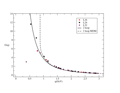
The two loop results for the Euclidean propagator are plotted together with the lattice results from [16] in fig. 8. Again we have set $\Lambda_{\overline{MS}}$=237 Mev and $\lambda_{g}$ was determined by fitting the two loop results on the lattice results at the highest lattice momentum ($\approx 5.5$ Gev, not shown in the fig.). Notice the Landau-pole for the MOM result. The agreement of our result with the lattice results is satisfying, apart from the strange single data point at the lowest lattice momentum. For the IR-behavior of our result we now find:

$$G(q)\stackrel{{\scriptstyle q\rightarrow 0}}{{\sim}}q^{-\frac{103}{68}}~{}~{},$$ (3.43)

which is more singular then the gluon propagator but less singular then the tree level result. Although this IR-behavior is consistent with [16], we should remark that other lattice studies [17, 18] predict a more singular behavior.

Figure 8: Lattice result taken from fig.1 in [16] (with $a^{-1}$=2 Gev) for the ghost propagator with the two loop results from the $y$-expansion and the MOM scheme, $\Lambda_{\overline{MS}}$=237Mev.

4 Conclusion

We have presented an alternative perturbative expansion for QCD with only one redundant parameter, fixed by a facc, and the unexpected feature of IR-finite results. The reason behind this was found to be a universal power behavior of the running expansion parameter $y$. For zero flavors there is a qualitative agreement with the lattice data, comparable with the Schwinger-Dyson results [19].

We do not expect our result to cover all the physics in the intermediate energy region and in the IR region. It is immediately clear for example, that the $y$-expansion for non-zero quark flavor will still respect the chiral symmetry, so additional non-perturbative corrections are definitely needed. However, the fact that our expansion gives finite results in the whole range of energies, seems to make it a better (then ordinary perturbation) framework to start from, if one wants to estimate the true non-perturbative corrections. In the future we will calculate such typical sum-rule quantities as current-current 2-point functions. Other possible applications are the calculation of experimental cross-sections, starting from the ordinary perturbation theory results.

Acknowledgements

We would like to thank the lattice community for providing us with some of their data. In particular we would like to thank P.Bowman, O.Pene, C.Pittori, J.Micheli and J.Skullerud. We also thank K.Chetyrkin for giving his (perturbative) data in several output formats. Finally we thank O.Bernus for the helping hand on the graphics.