Closed-Form Summation of RG-Accessible Logarithmic Contributions to Semileptonic B-Decays and Other Perturbative Processes

Abstract

For any perturbative series that is known to $k$-subleading orders of perturbation theory, we utilise the process-appropriate renormalization-group (RG) equation in order to obtain all-orders summation of series terms proportional to $\alpha^{n}\log^{n-k}\left(\mu^{2}\right)$ with $k=\{0,1,2,3\}$, corresponding to the summation to all orders of the leading and subsequent-three-subleading logarithmic contributions to the full perturbative series. These methods are applied to the perturbative series for semileptonic $b$-decays in both $\overline{{\rm MS}}$ and pole-mass schemes, and they result in RG-summed series for the decay rates which exhibit greatly reduced sensitivity to the renormalization scale $\mu$. Such summation via RG-methods of all logarithms accessible from known series terms is also applied to perturbative QCD series for vector- and scalar-current correlation functions, the perturbative static potential function, the (single-doublet standard-model) Higgs decay amplitude into two gluons, as well as the Higgs-mediated high-energy cross-section for $W^{+}W^{-}\to ZZ$ scattering. The resulting RG-summed expressions are also found to be much less sensitive to the renormalization scale than the original series for these processes.

1 Introduction

The renormalization group equation (RGE) has long proven useful as a means of improving and extending results obtained from perturbative quantum field theory. In addition to giving rise to scale-dependent running parameters (coupling constants and masses) and concomitant scale properties (e.g. asymptotic freedom), the RGE can also be utilised to determine scale-dependent portions of higher-order contributions to perturbative expressions. For example, if the two-loop contribution to a physical process has been determined via explicit computation of pertinent Feynman diagrams, the RGE then determines all leading-log and next-to-leading contributions to all subsequent orders of perturbation theory. We denote such logarithms to be “RG-accessible.” In the present paper we demonstrate how closed-form summation of such RG-accessible logarithm contributions is obtained for a number of physical processes whose field-theoretical series are known to two or more nonleading orders of perturbation theory.

Consider a perturbative series of the form

$$S[x(\mu),L(\mu)]=\sum_{n=0}^{\infty}x^{n}S_{n}\left[xL\right]=\sum_{n=0}^{\infty}\sum_{k=0}^{n}T_{n,k}x^{n}L^{k}$$ (1.1)

occurring within a physical decay rate $\Gamma$ or measurable cross-section $\sigma$, where $x(\mu)$ is the running coupling constant (for QCD $x(\mu)\equiv\alpha_{s}(\mu)/\pi$) and where $L(\mu)$ is a logarithm regulated by the renormalization mass scale $\mu$ that may or may not also depend on a running mass:

$$L(\mu)\equiv\log\left(\frac{\mu^{2}}{m^{2}}\right)$$ (1.2)

If $m$ is a running mass, then

$$\mu^{2}\frac{\mathrm{d}m}{\mathrm{d}\mu^{2}}=m\gamma_{m}[x(\mu)]=-m[\gamma_{0}x+\gamma_{1}x^{2}+\gamma_{2}x^{3}+...]$$ (1.3)

If $m$ is a pole mass (or for scattering processes, a kinematic variable), then $\gamma_{m}$ as defined by (1.3) is zero.

For example, in the fully $\overline{{\rm MS}}$ expression for the semileptonic $b\rightarrow u\ell^{-}\bar{\nu}_{\ell}$ rate obtained from five active flavours, $m$ is the running mass $m_{b}(\mu)$,

$$\Gamma=\frac{G_{F}^{2}|V_{ub}|^{2}}{192\pi^{3}}[m_{b}(\mu)]^{5}S[x(\mu),L(\mu)]$$ (1.4)

and the successive-order series coefficients within $S[x,L]$, as defined by (1.1), are [1]

$$T_{0,0}=1,\;T_{1,0}=4.25360,\;T_{1,1}=5,\;T_{2,0}=26.7848,\;T_{2,1}=36.9902,\;T_{2,2}=17.2917$$ (1.5)

The five active-flavour pole-mass expression for the same rate is obtained by replacing $m_{b}(\mu)$ with the renormalization-scale independent pole mass $m_{b}^{pole}$ in (1.4) and (1.2), as well as a concomitant alteration of the following series coefficients [1]

$$T_{1,0}=-2.41307,\;T_{1,1}=0,\;T_{2,0}=-21.2955,\;T_{2,1}=-4.62505,\;T_{2,2}=0.$$ (1.6)

Suppose for a given scattering or decay process that the series $S[x,L]$ is known to some order of perturbation theory:

$$S^{NL}=T_{0,0}+\left(T_{1,0}+T_{1,1}L\right)x$$ (1.7)

$$S^{NNL}=S^{NL}+\left(T_{2,0}+T_{2,1}L+T_{2,2}L^{2}\right)x^{2}$$ (1.8)

$$S^{N^{3}L}=S^{NNL}+\left(T_{3,0}+T_{3,1}L+T_{3,2}L^{2}+T_{3,3}L^{3}\right)x^{3}$$ (1.9)

$$S^{N^{4}L}=S^{N^{3}L}+\left(T_{4,0}+T_{4,1}L+T_{4,2}L^{2}+T_{4,3}L^{3}+T_{4,4}L^{4}\right)x^{4}.$$ (1.10)

These next-to-leading (NL) and higher-order expressions exhibit scale dependence as the magnitude of $L$ increases. However, higher order polynomial coefficients of $L$ can be determined via an appropriate RGE. For example, in $b\rightarrow u\ell^{-}\bar{\nu}_{\ell}$ the application of the RGE to the known [1] two-loop (NNL) $\overline{{\rm MS}}$ expression for the rate is sufficient to determine the three-loop coefficients $T_{3,3},\;T_{3,2},$ and $T_{3,1}$: for $n_{f}=5$, $T_{3,3}=50.914$, $T_{3,2}=178.76$, and $T_{3,1}=249.59$ [2]. This procedure is taken a step further in ref. [3], in which the four loop coefficients $T_{4,4},\;T_{4,3}$, and $T_{4,2}$ are determined via the RGE for this same process. Estimates for $T_{3,0}$ are also seen to determine $T_{4,1}$, yielding an $S^{N^{4}L}$ expression characterized by only two unknown coefficients ($T_{3,0}$ and $T_{4,0}$) whose parameter space can be limited by the constraint [3] that successive orders of perturbation theory decrease in magnitude

$$|S^{N^{4}L}-S^{N^{3}L}|\lesssim|S^{N^{3}L}-S^{N^{2}L}|\lesssim|S^{N^{2}L}-S^{NL}|.$$ (1.11)

In the present work, we wish to show how all RG-accessible logarithms may be summed if $S$ is known to a given order. Specifically, we shall obtain explicit all-orders summations for the following four series, as defined by the intermediate expression in (1.1):

$$S_{0}\left[x(\mu)L(\mu)\right]\equiv T_{0,0}+T_{1,1}xL+T_{2,2}x^{2}L^{2}+T_{3,3}x^{3}L^{3}+\ldots=\sum_{n=0}^{\infty}T_{n,n}x^{n}L^{n}$$ (1.12)

$$S_{1}\left[x(\mu)L(\mu)\right]\equiv T_{1,0}+T_{2,1}xL+T_{3,2}x^{2}L^{2}+\ldots=\sum_{n=1}^{\infty}T_{n,n-1}(xL)^{n-1}$$ (1.13)

$$S_{2}\left[x(\mu)L(\mu)\right]\equiv T_{2,0}+T_{3,1}xL+T_{4,2}x^{2}L^{2}+\ldots=\sum_{n=2}^{\infty}T_{n,n-2}(xL)^{n-2}$$ (1.14)

$$S_{3}\left[x(\mu)L(\mu)\right]\equiv T_{3,0}+T_{4,1}xL+T_{5,2}x^{2}L^{2}+\ldots=\sum_{n=3}^{\infty}T_{n,n-3}(xL)^{n-3}$$ (1.15)

The appropriate RGE $\left(\mu^{2}\frac{\mathrm{d}}{\mathrm{d}\mu^{2}}(\Gamma\;\mbox{or}\;\sigma)=0\right)$ is seen to determine all series coefficients of $S_{n}$ in terms of its leading coefficient $T_{n,0}$, thereby facilitating the construction of RG-summed (RG$\Sigma$) perturbative expressions to any given order of perturbation theory:

$$S_{RG\Sigma}^{NL}=S_{0}[xL]+xS_{1}[xL]$$ (1.16)

$$S_{RG\Sigma}^{NNL}=S_{0}[xL]+xS_{1}[xL]+x^{2}S_{2}[xL]$$ (1.17)

$$S_{RG\Sigma}^{N^{3}L}=S_{0}[xL]+xS_{1}[xL]+x^{2}S_{2}[xL]+x^{3}S_{3}[xL]$$ (1.18)

These ${\rm RG}\Sigma$ expressions are seen to exhibit reduced sensitivity to the renormalization scale $\mu$ even when the logarithms $L$ are quite large. Compared with the truncated perturbative series, these resummed expressions more effectively implement the underlying idea behind the RGE, namely that the exact (all-orders) expression for any physical quantity is necessarily independent of the scale-parameter $\mu$.

Although RGE determinations of higher-order terms have been known for some time to be of value in extracting divergent parts of bare parameters [4], the principle of incorporating all higher-order RG-accessible terms available to a given Feynman-diagram order of perturbation theory was, to the best of our knowledge, first articulated by Maxwell [5] as a method for eliminating unphysical renormalization-scale dependence. The all-orders summation of leading logarithms has been subsequently applied by Maxwell and Mirjalili [6] to moments of QCD leptoproduction structure functions and to ${\rm NNL}$-order correlation functions. Such a summation of leading-logarithm contributions to all orders has also been explicitly performed by McKeon to extract one-loop RG functions from the effective actions of $\phi^{4}$-field theory in four dimensions and $\phi^{6}$-field theories in three dimensions [7]. In Section 2 of the present work, we extend McKeon’s summation procedure to derive closed-form expressions for all-orders summations of leading- (1.12), NL-(1.13), NNL- (1.14), and ${\rm N^{3}L}$-logarithms (1.15) by using the RGE appropriate to the perturbative series (1.1) within the QCD expression for the inclusive semileptonic B-decay rate. Such summations enable one to construct ${\rm RG}\Sigma$ perturbative expressions inclusive of up-to-three nonleading logarithmic contributions to all orders of the perturbative series (1.1).

In Section 3, these results are applied to the $b\rightarrow u\ell^{-}\bar{\nu}_{\ell}$ rate computed to NNL order by van Ritbergen [1], later extended via Padé-approximant methods to a subsequent $N^{3}L$ prediction [2]. The renormalization-scale dependence of the unsummed perturbative rate truncated to a given order is shown to be much greater than that of the ${\rm RG}\Sigma$ rates obtained from the same perturbative expression.

In Section 4, ${\rm RG}\Sigma$ expressions are obtained for the decays $b\rightarrow u\ell^{-}\bar{\nu}_{\ell}$ and $b\rightarrow c\ell^{-}\bar{\nu}_{\ell}$ in the “pole mass” scheme in which only the couplant $\alpha_{s}(\mu)/\pi$ exhibits renormalization-scale dependence. This scheme, already known to have difficulties for the $b\rightarrow u$ case [1], exhibits a rate which increases with the renormalization scale $\mu$, making the identification of a “correct” or optimal value of $\mu$ problematical. However, RG-summation is shown effectively to remove such $\mu$-dependence, leading to reliable order-by-order pole-mass-scheme predictions for the $b\rightarrow u$ semileptonic rate consistent with the $b\rightarrow u$ rate obtained from an $\overline{{\rm MS}}$-scheme inclusive of a running b-quark mass. ${\rm RG}\Sigma$-expressions are also obtained for the $b\rightarrow c$ semileptonic rate based upon its (approximately-) known ${\rm NNL}$ series [8] and its Padé-estimated $N^{3}L$ series in the pole-mass scheme [9].

The RGE appropriate for the perturbative series for semileptonic B-decays in the pole mass scheme is also the appropriate RGE for the fermionic vector-current correlation function utilised to obtain QCD corrections to the cross-section ratio $\sigma(e^{+}e^{-}\rightarrow\mbox{hadrons})/\sigma(e^{+}e^{-}\rightarrow\mu^{+}\mu^{-})$. In Section 5 we obtain RG-summation expressions for the QCD series embedded within the vector-current correlation function that include all higher-order logarithmic contributions that are accessible from the three fully-known nonleading orders of perturbative corrections in the $\overline{{\rm MS}}$ scheme. We are thus able to compare directly the renormalization-scale dependence of the unsummed series $S^{NL}$ (1.7), $S^{NNL}$ (1.8), and $S^{N^{3}L}$ (1.9) to their corresponding ${\rm RG}\Sigma$ expressions $S_{RG\Sigma}^{NL}$ (1.16), $S_{RG\Sigma}^{NNL}$ (1.17), and $S_{RG\Sigma}^{N^{3}L}$ (1.18). We find that the latter expressions provide a set of virtually scale-independent order-by-order perturbative predictions for the vector correlator.

In Section 6, we show how the use of process-appropriate RGE’s can be used to obtain ${\rm RG}\Sigma$ perturbative expressions for a number of other processes. We obtain full RG-summations for

1. the momentum-space series for perturbative contributions to the QCD static-potential function,

2. the gluonic scalar-current correlation function characterising scalar gluonium states in QCD sum rules,

3. the (standard-model-) Higgs-mediated cross-section $W_{L}^{+}W_{L}^{-}\rightarrow Z_{L}Z_{L}$ at high energies, which is characterised by the two physical scale parameters $s$ and $M_{H}$,

4. the decay of a standard-model Higgs boson into two gluons [a process also characterised by two physical scales ($M_{H}$ and $M_{t}$) in addition to the renormalization scale $\mu$], and

5. the fermionic scalar-current correlation function that characterises both Higgs $\rightarrow b\bar{b}$ decays and scalar-meson-channel QCD sum rules.

We also discuss how RG-summation of the two scalar-current correlators considered in Section 6 removes much of the unphysical $\mu$-dependence of the unsummed series at low s that would otherwise percolate through QCD sum-rule integrals sensitive to the low-s region.

In Section 7 we summarise our paper. We discuss not only the reduction of $\mu$-dependence via RG-summation, but also the comparison of ${\rm RG}\Sigma$ results with those of unsummed series when minimal sensitivity or fastest apparent convergence is used to extract an optimal value for the renormalization scale.

Finally, an alternative all-orders summation procedure to that of Section 2 is presented in an appendix.

2 RG-Summation of Logarithms for Semileptonic B-Decays

For semileptonic b-decays, the $\mu$-sensitive portion of the rate (1.4) must, as a physically measurable quantity, exhibit renormalization scale-invariance:

$$\mu^{2}\frac{\mathrm{d}}{\mathrm{d}\mu^{2}}\left\{[m_{b}(\mu)]^{5}S[x(\mu),L(\mu)]\right\}=0.$$ (2.1)

This constraint is easily seen to lead to the RGE

$$\left[1-2\gamma_{m}(x)\right]\frac{\partial S}{\partial L}+\beta(x)\frac{\partial S}{\partial x}+5\gamma_{m}S=0,$$ (2.2)

where

$$\beta(x)\equiv\mu^{2}\frac{\mathrm{d}}{\mathrm{d}\mu^{2}}x(\mu)=-(\beta_{0}x^{2}+\beta_{1}x^{3}+\beta_{2}x^{4}+\ldots)\quad,$$ (2.3)

$[x(\mu)\equiv\alpha_{s}(\mu)/\pi]$ and where the anomalous mass dimension is the series defined by (1.3). Substitution of the series expansion (1.1) into the RGE yields the following series equation:

$$\begin{split}0=&\left(1+2\gamma_{0}x+2\gamma_{1}x^{2}+2\gamma_{2}x^{3}+\ldots\right)\sum_{n=0}^{\infty}\sum_{k=1}^{n}T_{n,k}kx^{n}L^{k-1}\\ &-\left(\beta_{0}x^{2}+\beta_{1}x^{3}+\beta_{2}x^{4}+\ldots\right)\sum_{n=1}^{\infty}\sum_{k=0}^{n}T_{n,k}nx^{n-1}L^{k}\\ &-5\left(\gamma_{0}x+\gamma_{1}x^{2}+\gamma_{2}x^{3}+\ldots\right)\sum_{n=0}^{\infty}\sum_{k=0}^{n}T_{n,k}x^{n}L^{k}\quad.\end{split}$$ (2.4)

2.1 Evaluation of $S_{0}$

To evaluate $S_{0}[xL]$, as defined by (1.12), we use (2.4) to extract the aggregate coefficient of $x^{n}L^{n-1}$ and to obtain the recursion formula $(n\geq 1)$

$$nT_{n,n}-\left[\beta_{0}(n-1)+5\gamma_{0}\right]T_{n-1,\;n-1}=0.$$ (2.5)

We multiply (2.5) by $u^{n-1}$ and sum from $n=1$ to $\infty$ to obtain the differential equation,

$$(1-\beta_{0}u)\frac{\mathrm{d}S_{0}[u]}{\mathrm{d}u}-5\gamma_{0}S_{0}[u]=0,$$ (2.6)

where $S_{0}[u]$ is given by (1.16) with $xL$ replaced by $u$. The solution of (2.6) for the initial condition $S_{0}[0]=T_{0,0}$ is

$$S_{0}[u]=T_{0,0}(1-\beta_{0}u)^{-5\gamma_{0}/\beta_{0}}.$$ (2.7)

For the special case of pole-mass renormalization schemes $[\gamma_{m}[x]=0]$, $S_{0}=T_{0,0}=1$, corresponding to the complete absence of $x^{n}L^{n}$ terms from the perturbative series (1.1) when $n\geq 1$.

2.2 Evaluation of $S_{1}$

To evaluate $S_{1}[u]$, as defined by (1.13) with $u=x(\mu)L(\mu)$ we first extract the aggregate coefficient of $x^{n}L^{n-2}$ from the RGE (2.4) for $n\geq 2$:

$$\begin{split}0=&(n-1)T_{n,\;n-1}+2\gamma_{0}(n-1)T_{n-1,\;n-1}-\beta_{0}(n-1)T_{n-1,\;n-2}\\ &-\beta_{1}(n-2)T_{n-2,\;n-2}-5\gamma_{0}T_{n-1,\;n-2}-5\gamma_{1}T_{n-2,\;n-2}\quad.\end{split}$$ (2.8)

If one multiplies (2.8) by $u^{n-2}$ and then sums from $n=2$ to infinity, one obtains the differential equation

$$(1-\beta_{0}u)\frac{\mathrm{d}S_{1}}{\mathrm{d}u}-(\beta_{0}+5\gamma_{0})S_{1}[u]=5\gamma_{1}S_{0}[u]+(\beta_{1}u-2\gamma_{0})\frac{\mathrm{d}S_{0}}{\mathrm{d}u}.$$ (2.9)

We find it convenient to re-express this equation in terms of the variable

$$w\equiv 1-\beta_{0}u$$ (2.10)

and the constant

$$A\equiv\frac{5\gamma_{0}}{\beta_{0}}.$$ (2.11)

We see from (2.7) that if $T_{0,0}=1$, then

$$S_{0}=w^{-A}$$ (2.12)

and find from (2.9) the following differential equation for $S_{1}$:

$$\frac{\mathrm{d}S_{1}}{\mathrm{d}w}+\frac{1+A}{w}S_{1}=Bw^{-A-1}+Cw^{-A-2}$$ (2.13)

where

$$B\equiv\left(A\beta_{1}-5\gamma_{1}\right)/\beta_{0}$$ (2.14)

$$C\equiv A\left(2\gamma_{0}-\beta_{1}/\beta_{0}\right).$$ (2.15)

For initial condition $S_{1}|_{u=0}=S_{1}|_{w=1}=T_{1,0}$, the solution to (2.13) is

$$S_{1}=Bw^{-A}+\left[T_{1,0}-B+C\log(w)\right]w^{-A-1}$$ (2.16)

with $w,A,B$ and $C$ respectively given by (2.10), (2.11), (2.14) and (2.15).

2.3 Evaluation of $S_{2}$

The aggregate coefficient of $x^{n}L^{n-3}$ in eq. (2.4) is $(n\geq 3)$

$$\begin{split}0=&(n-2)T_{n,n-2}+2\gamma_{0}(n-2)T_{n-1,\;n-2}+2\gamma_{1}(n-2)T_{n-2,\;n-2}-\beta_{0}(n-1)T_{n-1,\;n-3}\\ &-\beta_{1}(n-2)T_{n-2,\;n-3}-\beta_{2}(n-3)T_{n-3,\;n-3}-5\gamma_{0}T_{n-1,\;n-3}-5\gamma_{1}T_{n-2,\;n-3}-5\gamma_{2}T_{n-3,\;n-3}\quad.\end{split}$$ (2.17)

If one multiplies (2.17) by $u^{n-3}$ and sums from $n=3$ to infinity, one finds from the definitions

$$S_{0}[u]=1+\sum_{n=1}^{\infty}T_{n,n}u^{n},$$ (2.18)

$$S_{1}[u]=\sum_{n=1}^{\infty}T_{n,n-1}u^{n-1},$$ (2.19)

$$S_{2}[u]=\sum_{n=2}^{\infty}T_{n,n-2}u^{n-2}$$ (2.20)

[following from (1.12–1.14)] that

$$\frac{\mathrm{d}S_{2}}{\mathrm{d}u}-\frac{\left(2\beta_{0}+5\gamma_{0}\right)}{1-\beta_{0}u}S_{2}=\frac{\left(\beta_{1}u-2\gamma_{0}\right)}{1-\beta_{0}u}\frac{\mathrm{d}S_{1}}{\mathrm{d}u}+\frac{\left(\beta_{2}u-2\gamma_{1}\right)}{1-\beta_{0}u}\frac{\mathrm{d}S_{0}}{\mathrm{d}u}+\frac{\left(\beta_{1}+5\gamma_{1}\right)}{1-\beta_{0}u}S_{1}+\frac{5\gamma_{2}}{1-\beta_{0}u}S_{0}\quad.$$ (2.21)

If we incorporate the change-of-variable (2.10) in conjunction with the solutions (2.12) and (2.16) for $S_{0}$ and $S_{1}$, respectively, we find that

$$\frac{\mathrm{d}S_{2}}{\mathrm{d}w}+\frac{(2+A)}{w}S_{2}=Dw^{-A-1}+Ew^{-A-2}+Fw^{-A-2}\log(w)+Gw^{-A-3}+Hw^{-A-3}\log(w)\quad,$$ (2.22)

where the constants $\{D,E,F,G,H\}$ are given by

$$D=\left[\beta_{1}AB+\beta_{2}A-\left(\beta_{1}+5\gamma_{1}\right)B-5\gamma_{2}\right]/\beta_{0}$$ (2.23)

$$E=\left(2\gamma_{0}-\frac{\beta_{1}}{\beta_{0}}\right)AB+\left[(1+A)\left(T_{1,0}-B\right)-C\right]\frac{\beta_{1}}{\beta_{0}}+\left(2\gamma_{1}-\frac{\beta_{2}}{\beta_{0}}\right)A+\left(B-T_{1,0}\right)\left(\beta_{1}+5\gamma_{1}\right)/\beta_{0}$$ (2.24)

$$F=\left(A\beta_{1}-5\gamma_{1}\right)C/\beta_{0}$$ (2.25)

$$G=\left[(1+A)\left(T_{1,0}-B\right)-C\right]\left(2\gamma_{0}-\frac{\beta_{1}}{\beta_{0}}\right)$$ (2.26)

$$H=\left(2\gamma_{0}-\frac{\beta_{1}}{\beta_{0}}\right)(1+A)C$$ (2.27)

with constants $\{A,B,C\}$ given by (2.11), (2.14) and (2.15). The solution to the differential equation (2.21) with initial condition $S_{2}|_{u=0}=S_{2}|_{w=1}=T_{2,0}$ is

$$\begin{split}S_{2}=&\frac{D}{2}w^{-A}+(E-F)w^{-A-1}+Fw^{-A-1}\log(w)+\left(T_{2,0}-\frac{D}{2}-E+F\right)w^{-A-2}\\ &+Gw^{-A-2}\log(w)+\frac{H}{2}w^{-A-2}\log^{2}(w).\end{split}$$ (2.28)

2.4 Evaluation of $S_{3}$

The aggregate coefficient of $x^{n}L^{n-4}$ in (2.4) is

$$\begin{split}0=&(n-3)\left[T_{n,n-3}+2\gamma_{0}T_{n-1,\;n-3}+2\gamma_{1}T_{n-2,\;n-3}+2\gamma_{2}T_{n-3,\;n-3}\right]\\ &-\beta_{0}(n-1)T_{n-1,\;n-4}-\beta_{1}(n-2)T_{n-2,\;n-4}-\beta_{2}(n-3)T_{n-3,\;n-4}-\beta_{3}(n-4)T_{n-4,\;n-4}\\ &-5\gamma_{0}T_{n-1,\;n-4}-5\gamma_{1}T_{n-2,\;n-4}-5\gamma_{2}T_{n-3,\;n-4}-5\gamma_{3}T_{n-4,\;n-4}\quad.\end{split}$$ (2.29)

To evaluate the series

$$S_{3}[u]=\sum_{n=3}^{\infty}T_{n,n-3}u^{n-3}.$$ (2.30)

we multiply (2.29) by $u^{n-4}$, sum from $n=4$ to infinity, and, as before, make the eq. (2.10) change of variable $w=1-\beta_{0}u$. We then find that

$$\begin{split}\frac{\mathrm{d}S_{3}}{\mathrm{d}w}+\frac{3+A}{w}S_{3}=&Kw^{-A-1}+Mw^{-A-2}+Nw^{-A-2}\log(w)+Pw^{-A-3}+Qw^{-A-3}\log(w)\\ &+Rw^{-A-3}\log^{2}(w)+Uw^{-A-4}+Vw^{-A-4}\log(w)+Yw^{-A-4}\log^{2}(w)\quad,\end{split}$$ (2.31)

by utilizing the explicit solutions (2.12), (2.16) and (2.28) for $\{S_{0},S_{1},S_{2}\}$, as defined by (2.18), (2.19) and (2.20). The new constants within (2.31) are

$$K=\frac{A}{\beta_{0}}\left(\beta_{3}+B\beta_{2}+D\beta_{1}/2\right)-\frac{1}{\beta_{0}}\left[5\gamma_{3}+\left(5\gamma_{2}+\beta_{2}\right)B+\left(5\gamma_{1}+2\beta_{1}\right)\frac{D}{2}\right]$$ (2.32)

$$\begin{split}M=&\left[\left(2\gamma_{2}-\frac{\beta_{3}}{\beta_{0}}\right)+\left(2\gamma_{1}-\frac{\beta_{2}}{\beta_{0}}\right)B+\left(2\gamma_{0}-\frac{\beta_{1}}{\beta_{0}}\right)\frac{D}{2}\right]A\\ &+\left[\left(5\gamma_{2}+\beta_{2}\right)\left(B-T_{1,0}\right)+\left(5\gamma_{1}+2\beta_{1}\right)(F-E)\right]\frac{1}{\beta_{0}}\\ &+\left[\left(T_{1,0}-B\right)(1+A)-C\right]\frac{\beta_{2}}{\beta_{0}}+\left[E(1+A)-F(2+A)\right]\frac{\beta_{1}}{\beta_{0}}\end{split}$$ (2.33)

$$N=\left\{\left(A\beta_{2}-5\gamma_{2}\right)C+\left[(A-1)\beta_{1}-5\gamma_{1}\right]F\right\}\frac{1}{\beta_{0}}$$ (2.34)

$$\begin{split}P=&\left(2\gamma_{1}-\frac{\beta_{2}}{\beta_{0}}\right)\left[(1+A)\left(T_{1,0}-B\right)-C\right]+\left(2\gamma_{0}-\frac{\beta_{1}}{\beta_{0}}\right)\left[(1+A)E-(2+A)F\right]\\ &-\frac{\left(5\gamma_{1}+2\beta_{1}\right)}{\beta_{0}}\left(T_{2,0}-\frac{D}{2}-E+F\right)-\frac{\beta_{1}}{\beta_{0}}\left[G-(2+A)\left(T_{2,0}-\frac{D}{2}-E+F\right)\right]\end{split}$$ (2.35)

$$Q=\left[\left(2\gamma_{1}-\frac{\beta_{2}}{\beta_{0}}\right)C+\left(2\gamma_{0}-\frac{\beta_{1}}{\beta_{0}}\right)F\right](1+A)-\left[\left(5\gamma_{1}+2\beta_{1}\right)G+(H-(2+A)G)\beta_{1}\right]\frac{1}{\beta_{0}}$$ (2.36)

$$R=\left(\beta_{1}A-5\gamma_{1}\right)\frac{H}{2\beta_{0}}$$ (2.37)

$$U=\left(2\gamma_{0}-\frac{\beta_{1}}{\beta_{0}}\right)\left[(2+A)\left(T_{2,0}-\frac{D}{2}-E+F\right)-G\right]$$ (2.38)

$$V=\left(2\gamma_{0}-\frac{\beta_{1}}{\beta_{0}}\right)\left[(2+A)G-H\right]$$ (2.39)

$$Y=\left(2\gamma_{0}-\frac{\beta_{1}}{\beta_{0}}\right)(2+A)\frac{H}{2}\quad.$$ (2.40)

The constants $\{A,B,C,D,E,F,G,H\}$ within (2.31) are respectively given by {(2.11), (2.14), (2.15), (2.23–2.27)}. The solution to (2.31), subject to the initial condition $S_{3}|_{w=1}=T_{3,0}$, is

$$\begin{split}S_{3}=&\frac{K}{3}w^{-A}+\left(\frac{M}{2}-\frac{N}{4}\right)w^{-A-1}+\frac{N}{2}w^{-A-1}\log(w)+(P-Q+2R)w^{-A-2}+(Q-2R)w^{-A-2}\log(w)\\ &+Rw^{-A-2}\log^{2}(w)+\left(-\frac{K}{3}-\frac{M}{2}+\frac{N}{4}-P+Q-2R+T_{3,0}\right)w^{-A-3}\\ &+Uw^{-A-3}\log(w)+\frac{V}{2}w^{-A-3}\log^{2}(w)+\frac{Y}{3}w^{-A-3}\log^{3}(w)\quad,\end{split}$$ (2.41)

where $w=1-\beta_{0}u$ as in (2.10).

3 Semileptonic $b\rightarrow u\ell^{-}\bar{\nu}_{\ell}$ Decay in the $\overline{{\rm MS}}$ Scheme

In this section, we consider the semileptonic decay $b\rightarrow u\ell^{-}\bar{\nu}_{\ell}$ in the $\overline{\rm{MS}}$ scheme. The decay rate is given by (1.4) in terms of the series (1.1). The coefficients in this series are fully known to two loop order and are given by (1.5). The logarithms $L(\mu)$ within the series are characterized by a running $b$-quark mass, as given by (1.2) and (1.3).

The coefficients (1.5) are listed for five active flavours, appropriate to analysis in an energy region containing $m_{b}(m_{b})$. Consequently, the running $b$-quark mass $m_{b}(\mu)$ and the running couplant $x(\mu)=\alpha_{s}(\mu)/\pi$ should be characterized by $n_{f}=5$ values for the RG functions $\gamma_{m}[x]$ and $\beta[x]$:

$$\gamma_{0}=1,\;\gamma_{1}=\frac{253}{72},\;\gamma_{2}=7.41986,\;\gamma_{3}=11.0343$$ (3.1)

$$\beta_{0}=\frac{23}{12},\;\beta_{1}=\frac{29}{12},\;\beta_{2}=\frac{9769}{3456},\;\beta_{3}=18.8522$$ (3.2)

Given the computed values of $T_{1,0}$ and $T_{2,0}$ [1], it is straightforward to calculate the ${\rm NL}$ and ${\rm NNL}$ RG-summations for the series $S$, as defined in (1.16) and (1.17). The constants $\{A,B,C,\ldots,H\}$ that characterise the summations $S_{0},S_{1}$ and $S_{2}$ are obtained via (3.1), (3.2) and (1.5) from their definitions in Section 2:

$$\begin{split}A=&\frac{60}{23},\;\;B=-\frac{18655}{3174},\;\;C=\frac{1020}{529},\;\;D=26.4461,\\ E=&-58.8224,\;\;F=-\frac{3171350}{279841},\;\;G=25.5973,\;\;H=\frac{1439220}{279841}\quad.\end{split}$$ (3.3)

Eqs. (2.12), (2.16) and (2.28) then lead to the following closed-form expressions for the summations $S_{0}$, $S_{1}$ and $S_{2}$:

$$S_{0}=\left[1-\frac{23}{12}x(\mu)L(\mu)\right]^{-60/23}$$ (3.4)

$$\begin{split}S_{1}=&-\frac{18655}{3174}\left[1-\frac{23}{12}x(\mu)L(\mu)\right]^{-60/23}\\ +&\left\{10.1310+\frac{1020}{529}\log\left[1-\frac{23}{12}x(\mu)L(\mu)\right]\right\}\left[1-\frac{23}{12}x(\mu)L(\mu)\right]^{-83/23}\end{split}$$ (3.5)

$$\begin{split}S_{2}=&13.2231\left[1-\frac{23}{12}x(\mu)L(\mu)\right]^{-60/23}\\ &-\left\{47.4897+\frac{3171350}{279841}\log\left[1-\frac{23}{12}x(\mu)L(\mu)\right]\right\}\left[1-\frac{23}{12}x(\mu)L(\mu)\right]^{-83/23}\\ &+\left\{61.0515+25.5973\log\left[1-\frac{23}{12}x(\mu)L(\mu)\right]+\frac{719610}{279841}\log^{2}\left[1-\frac{23}{12}x(\mu)L(\mu)\right]\right\}\left[1-\frac{23}{12}x(\mu)L(\mu)\right]^{-106/23}\end{split}$$ (3.6)

We first wish to compare the $\mu$-dependence of the 2-loop order expression

$$\frac{\Gamma^{NNL}}{{\cal K}}=\left[m_{b}(\mu)\right]^{5}\left[1+(4.25360+5L(\mu))x(\mu)+\left(26.7848+36.9902L(\mu)+17.2917L^{2}(\mu)\right)x^{2}(\mu)\right]$$ (3.7)

for the reduced rate $\left({\cal K}\equiv G_{F}^{2}|V_{ub}|^{2}/192\pi^{3}\right)$ to that of the corresponding RG-summed expression

$$\frac{\Gamma_{RG\Sigma}^{NNL}}{{\cal K}}=[m_{b}(\mu)]^{5}\left[S_{0}+S_{1}x(\mu)+S_{2}x^{2}(\mu)\right]$$ (3.8)

with $S_{0},~{}S_{1}$ and $S_{2}$ given by (3.4), (3.5) and (3.6). To make this comparison, we evolve the running coupling and mass from initial values $x(4.17\,{\rm GeV})=0.0715492$ and $m_{b}(4.17\,{\rm GeV})=4.17\,{\rm GeV}$ [2], where the former value arises from $n_{f}=5$ evolution of the running coupling from an assumed anchoring value $x\left(M_{Z}\right)=0.118000/\pi$ [10], and where the latter value is the $n_{f}=5$ central value in ref. [11] for $m_{b}(m_{b})$. Thus $x(\mu)$, $m_{b}(\mu)$ and $L(\mu)$ are fully determined via (1.2) and the RG-equations (1.3) and (2.3), with $\gamma_{m}$- and $\beta$- function coefficients given by (3.1) and (3.2).

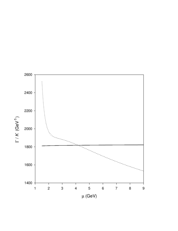
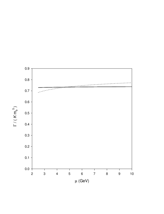
In Figure 1, we use the $n_{f}=5$ evolution of $x(\mu)$ and $m_{b}(\mu)$, as described above, to compare $\Gamma^{NNL}$ (3.7) to $\Gamma_{RG\Sigma}^{NNL}$ (3.8). It is clear from the figure that $\Gamma_{RG\Sigma}^{NNL}$ is almost perfectly flat. By contrast, the naive rate $\Gamma^{NNL}$ is strikingly dependent on the renormalization scale $\mu$, and does not exhibit any local extremum point of minimal sensitivity. Thus, RG-summation of leading, next-to-leading and next-to-next-to-leading logarithms is seen to remove the substantial theoretical uncertainty associated with the choice of $\mu$ from the (fully known) two-loop order $b\rightarrow u\ell^{-}\bar{\nu}_{\ell}$ rate.

It is useful to examine how the reduced $b\rightarrow u\ell^{-}\bar{\nu}_{\ell}$ rate develops in successive orders of perturbation theory. For example, the one-loop rates

$$\frac{\Gamma^{NL}}{{\cal K}}=\left[m_{b}(\mu)\right]^{5}\left[1+(4.25360+5L(\mu))x(\mu)\right]$$ (3.9)

$$\frac{\Gamma_{RG\Sigma}^{NL}}{{\cal K}}=\left[m_{b}(\mu)\right]^{5}\left[S_{0}+S_{1}x(\mu)\right]$$ (3.10)

can be compared to the corresponding higher precision results of eq. (3.7) and (3.8). Three-loop order $(N^{3}L)$ reduced rates can be estimated through incorporation of an asymptotic Padé-approximant prediction of the three-loop coefficient $T_{3,0}=206$ [2]. The three-loop order expression for the reduced rate

$$\begin{split}\frac{\Gamma^{N^{3}L}}{{\cal K}}=\left[m_{b}(\mu)\right]^{5}&\Biggl{\{}1+(4.25360+5L(\mu))x(\mu)+\left(26.7848+36.9902L(\mu)+17.2917L^{2}(\mu)\right)x^{2}(\mu)\Biggr{.}\\ &\quad+\Biggl{.}\left(206+249.592L(\mu)+178.755L^{2}(\mu)+50.9144L^{3}(\mu)\right)x^{3}(\mu)\Biggr{\}}\end{split}$$ (3.11)

can then be compared to its RG-summation version

$$\frac{\Gamma_{RG\Sigma}^{N^{3}L}}{{\cal K}}=\left[m_{b}(\mu)\right]^{5}\left[S_{0}+S_{1}x(\mu)+S_{2}x^{2}(\mu)+S_{3}x^{3}(\mu)\right]$$ (3.12)

with $S_{0}$, $S_{1}$ and $S_{2}$ respectively given by (3.4), (3.5) and (3.6). The RG-summation $S_{3}$, is obtained via (2.41). Given the estimate $T_{3,0}=206$, the known values (3.3) of $\{A,B,\ldots,H\}$ and values of $\{K,M,N,P,\ldots,Y\}$ defined via (2.32)–(2.40),

$$\begin{split}K&=-14.3686,\;M=146.729,\;N=50.9925,\;P=-317.085,\;Q=-148.520,\\ R&=-15.1138,\;U=189.048,\;V=83.3941,\;Y=8.75961,\end{split}$$ (3.13)

we find that

$$\begin{split}S_{3}=&-\frac{4.7895}{(1-\frac{23}{12}xL)^{60/23}}+\frac{[60.617+25.496\log(1-\frac{23}{12}xL)]}{(1-\frac{23}{12}xL)^{83/23}}\\ &+\frac{[-198.79-118.29\log(1-\frac{23}{12}xL)-15.114\log^{2}(1-\frac{23}{12}xL)]}{(1-\frac{23}{12}xL)^{106/23}}\\ &+\frac{[{\bf 348.96}+189.05\log(1-\frac{23}{12}xL)+41.697\log^{2}(1-\frac{23}{12}xL)+2.9199\log^{3}(1-\frac{23}{12}xL)]}{(1-\frac{23}{12}xL)^{129/23}}\end{split}$$ (3.14)

The bold-face number 348.96 is the only coefficient in the above expression dependent upon the asymptotic Padé-approximant estimate for $T_{3,0}$. We have included this estimate in order to demonstrate RG-summation incorporating a three-loop diagrammatic contribution to $T_{3,0}$; when such a calculation is performed, the factor 348.96 in (3.14) should then be replaced by $T_{3,0}+142.96$.

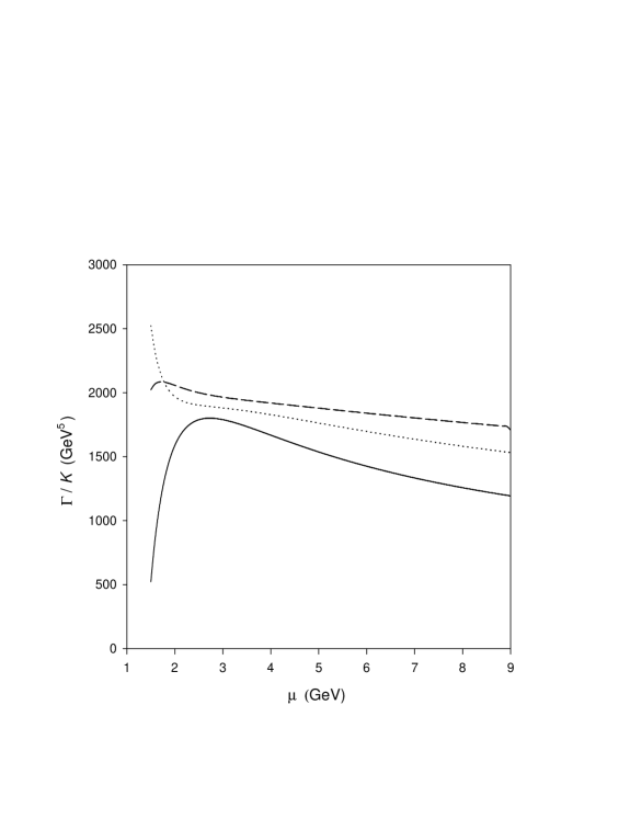
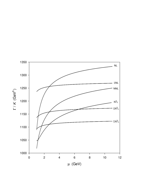
We consider the $\mu$-dependence of three non-leading orders of perturbation theory first for the case in which logarithms are not summed to all orders. Figure 2 displays a comparison of the “unsummed” one-, two- and three-loop order reduced rates $\Gamma^{NL}/{\cal K}$, $\Gamma^{NNL}/{\cal K}$ and $\Gamma^{N^{3}L}/{\cal K}$, respectively given by (3.9), (3.7) and (3.11). The $\mu$-dependence of all three orders is evident from the figure. Such $\mu$-dependence can be used to extract ${\rm NL}$ and $N^{3}L$ values for $\Gamma$ via the minimal-sensitivity criterion of ref. [12]. Curiously, $\Gamma^{NL}$ and $\Gamma^{N^{3}L}$ are both seen to have comparable minimal-sensitivity extrema ($1801\,{\rm GeV}^{5}$ and $2085\,{\rm GeV}^{5}$) at values of $\mu$ much less than $m_{b}(m_{b})$. $\Gamma^{NNL}$ exhibits some flattening between these extrema ($\approx 1900\,{\rm GeV}^{5}$) over the same range of $\mu$, but with a continued negative slope. Indeed, one can employ fastest apparent convergence [13] to choose $\mu$ for $\Gamma^{NNL}$ such that $|\Gamma^{NNL}(\mu)-\Gamma^{NL}(\mu)|$ is a minimum, and to choose $\mu$ for $\Gamma^{N^{3}L}$ such that$|\Gamma^{N^{3}L}(\mu)-\Gamma^{NNL}(\mu)|=0$. As evident from Fig. 2, the former criterion leads to a value for $\mu$ ($2.85\,{\rm GeV}$) quite close to that value at which $\Gamma^{NL}(\mu)$ has an extremum ($2.7\,{\rm GeV}$), corresponding to $\Gamma^{NNL}/{\cal K}=1888\,{\rm GeV}^{5}$. The latter criterion indicates that $\Gamma^{N^{3}L}$ should be evaluated at the point where $\Gamma^{NNL}$ and $\Gamma^{N^{3}L}$ cross, a point noted previously [2] to be virtually indistinguishable from the minimal-sensitivity extremum for $\Gamma^{N^{3}L}(\mu)$.

The point we wish to make here, however, is that all such values extracted for $\mu$ differ substantially from $m_{b}(m_{b})$, in which case progressively large powers of large-logarithms $L(\mu)\equiv\log[\mu^{2}/m_{b}^{2}(\mu)]$ enter the successive expressions (3.9), (3.7) and (3.11) for the ${\rm NL}$, ${\rm NNL}$ and $N^{3}L$ rate $\Gamma$. Moreover, in the absence of minimal-sensitivity or fastest-apparent-convergence criteria for extracting $\mu$, even the $N^{3}L$ rate exhibits a $\pm 8\%$ spread of values over the range $m_{b}/2\lesssim\mu\stackrel{{\scriptstyle<}}{{{}_{\sim}}}2m_{b}$.

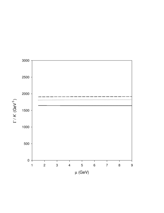
RG-summation eliminates renormalization scale-dependence as a cause of theoretical uncertainty. In Figure 3, we compare RG-summed versions of the reduced rate $\Gamma_{RG\Sigma}^{NL}$ (3.10), $\Gamma_{RG\Sigma}^{NNL}$ (3.8) and $\Gamma_{RG\Sigma}^{N^{3}L}$ (3.12). These three rates exhibit virtually no $\mu$ dependence whatsoever; rather, RG-summation is seen to lead to clear order-by-order predictions of the rate that are insensitive to $\mu$. We see from Fig. 3 that $\Gamma_{RG\Sigma}^{NL}/{\cal K}=1646\pm 2\,{\rm GeV}^{5}$, $\Gamma_{RG\Sigma}^{NNL}/{\cal K}=1816\pm 6\,{\rm GeV}^{5}$, and $\Gamma_{RG\Sigma}^{N^{3}L}/{\cal K}=1912\pm 4\,{\rm GeV}^{5}$ over the (more or less) physical range of $\mu$ considered in Fig. 3. Theoretical uncertainty in the calculated rate is now almost entirely attributable to truncation of the perturbation series to known contributions, an error which is seen to diminish as the order of known contributions increases.

It is important to realize, however, that these scale-independent predictions necessarily coincide with the $L(\mu)=0$ predictions of the unsummed rates (3.9), (3.7) and (3.11): $\Gamma^{N^{k}L}$ and $\Gamma_{RG\Sigma}^{N^{k}L}$ equilibrate when $w=1$ i.e., when $L(\mu)=0$. Thus, one can argue that the summation we have performed here of all RG-accessible logarithms supports the prescription of identifying as “physical” those perturbative results in which $\mu$-sensitive logarithms are set equal to zero. We must nevertheless recognize the possibility that the $\mu$-sensitivity of the unsummed rates, when exploited by minimal-sensitivity or fastest-apparent-convergence criteria, is capable of leading to more accurate order-by-order estimates of the true rate than corresponding scale-independent ${\rm RG}\Sigma$ rates. In comparing Figs. 2 and 3, it is noteworthy that the $1801\,{\rm GeV}^{5}$ extremum of $\Gamma^{NL}/{\cal K}$, the unsummed one-loop rate, is quite close to $\Gamma_{RG\Sigma}^{NNL}/{\cal K}$, the RG-summed two-loop rate. Similarly, the $1888\,{\rm GeV}^{5}$ fastest-apparent-convergence value of $\Gamma^{NNL}/{\cal K}$, the unsummed two-loop rate, is close to $\Gamma_{RG\Sigma}^{N^{3}L}$. This train of argument would suggest that the ${\cal{O}}(2085\,{\rm GeV}^{5})$ extremum (or fastest-apparent-convergence value) of the unsummed rate $\Gamma^{N^{3}L}/{\cal K}$ may be a more accurate estimate of the true rate than $\Gamma_{RG\Sigma}^{N^{3}L}$. Such an argument, however, requires substantiation via explicit three- and four-loop order calculations, computations which are not yet available.

4 Application to Semileptonic B decays in the Pole-Mass Scheme

In the pole-mass renormalization scheme, the mass $m$ appearing in logarithms (1.2) is independent of the renormalization mass-scale $\mu$. Thus the coefficients $\gamma_{k}$, as defined in (1.3) are all zero. The constants $\{A,B,C,D,E,F,H,$ $K,M,N,Q,R,Y\}$, as defined in Section 2, are all zero as well. The nonzero constants are

$$G=-T_{1,0}\frac{\beta_{1}}{\beta_{0}}$$ (4.1)

$$P=-T_{1,0}\left(\beta_{2}-\frac{\beta_{1}^{2}}{\beta_{0}}\right)\frac{1}{\beta_{0}}$$ (4.2)

$$U=\left[-T_{1,0}\frac{\beta_{1}}{\beta_{0}}-2T_{2,0}\right]\frac{\beta_{1}}{\beta_{0}}$$ (4.3)

$$V=2T_{1,0}\frac{\beta_{1}^{2}}{\beta_{0}^{2}}$$ (4.4)

and the corresponding RGE summations appearing within $S_{RG\Sigma}^{NL},S_{RG\Sigma}^{NNL}$, and $S_{RG\Sigma}^{N^{3}L}$ [(1.16), (1.17) and (1.18)] are

$$S_{0}=1$$ (4.5)

$$S_{1}[xL]=T_{1,0}/(1-\beta_{0}xL)$$ (4.6)

$$S_{2}[xL]=T_{2,0}(1-\beta_{0}xL)^{-2}+G(1-\beta_{0}xL)^{-2}\log(1-\beta_{0}xL)$$ (4.7)

$$S_{3}[xL]=P(1-\beta_{0}xL)^{-2}+\left[(T_{3,0}-P)+U\log(1-\beta_{0}xL)+\frac{V}{2}\log^{2}(1-\beta_{0}xL)\right](1-\beta_{0}xL)^{-3}\quad.$$ (4.8)

In this section, we apply the above results toward the decay $b\rightarrow u\ell^{-}\bar{\nu}_{\ell}$ and $b\rightarrow c\ell^{-}\bar{\nu}_{\ell}$. The former rate is known fully to two-loop order in the pole mass scheme, though the result is argued to be of limited phenomenological utility [1]. The latter rate has been estimated within fairly narrow errors to two-loop order as well [8], and has been extended to a three-loop order estimated rate via asymptotic Padé-approximate methods [9].

4.1 Pole Scheme Semileptonic $b\rightarrow u\ell^{-}\bar{\nu}_{\ell}$ Decay

The two-loop order $b\rightarrow u\ell^{-}\bar{\nu}_{\ell}$ rate in the pole mass scheme is given by substitution of known values of the coefficients $\{T_{1,0},T_{1,1},T_{2,0},T_{2,1},T_{2,2}\}$, as listed in (1.6) into the series (1.4), with $m_{b}(\mu)$ replaced by $m_{b}^{pole}$ as noted earlier. Although the reliability of the pole-mass scheme for this process is suspect because of the proximity of a renormalon pole [1], we have plotted this series for a range of $x(\mu)=\alpha_{s}(\mu)/\pi$ and a choice for $m_{b}^{pole}$ that will facilitate comparison with phenomenology already obtained from the corresponding $\overline{\rm{MS}}$ process. We choose $n_{f}=5$ active flavours in order to explore the $\mu$-dependence of the NNL rate in a region in which $\mu$ is considerably larger than $m_{b}^{pole}$. Corresponding results for four active flavours are easily obtainable as well. The evolution of $x(\mu)=\alpha_{s}(\mu)/\pi$ for five active flavours ultimately devolves from $\alpha_{s}(M_{z})=0.118$ and leads to the same $n_{f}=5$ benchmark value $x(4.17\,{\rm GeV})=0.071549$ as noted in Section 3. Similarly we employ a value for $m_{b}^{pole}=4.7659$ consistent to two-loop order with our use of the running mass value $m_{b}(m_{b})=4.17\,{\rm GeV}$, as obtained from the $n_{f}=5$ relation between $m_{b}^{pole}$ and $m_{b}(m_{b})$ of refs. [11, 14]:

$$m_{b}^{pole}=4.17\,{\rm GeV}\left[1+\frac{4}{3}x(4.17)+9.27793x^{2}(4.17)\right]$$ (4.9)

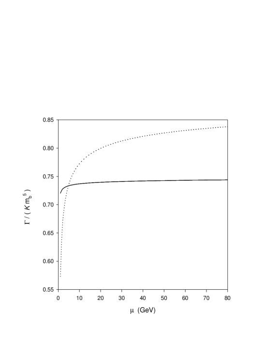
We then see from Fig. 4 that the $\mu$-sensitive portion of the known two-loop rate in the pole mass scheme,

$$S^{NNL}(\mu)=1-2.41307x(\mu)+\left[-21.2955-4.62505\log\left\{\left(\frac{\mu}{m_{b}^{pole}}\right)^{2}\right\}\;\right]x^{2}(\mu)$$ (4.10)

is indeed highly scale dependent. Specifically, we see that $S^{NNL}(\mu)$ increases monotonically with $\mu$ without exhibiting an extremum identifiable with a “physical” point of minimal sensitivity [12].

In Figure 4 we have also plotted the RG-summed version of the 2-loop rate

$$S_{RG\Sigma}^{NNL}=1+x(\mu)S_{1}\left[x(\mu)\log\left\{\left(\frac{\mu}{m_{b}^{pole}}\right)^{2}\right\}\right]+x^{2}(\mu)S_{2}\left[x(\mu)\log\left\{\left(\frac{\mu}{m_{b}^{pole}}\right)^{2}\right\}\right]$$ (4.11)

with $x(\mu)$ and $m_{b}^{pole}$ as obtained above. The summations $S_{1}$ and $S_{2}$ are obtained via (4.6) and (4.7) using the $n_{f}=5$ pole-mass scheme values $T_{1,0}=-2.41307$, $T_{2,0}=-21.2955$ [1] and $n_{f}=5$ QCD $\beta$-function coefficients $\beta_{0}=23/12$, $\beta_{1}=29/12$, and $\beta_{2}=9769/3456$. It is evident from the figure that renormalization scale-dependence is considerably reduced by the summation of all orders of leading and next-to-leading logarithms in (3.11). The increase of $S_{RG\Sigma}^{NNL}$ with increasing $\mu$ is minimal compared to that of $S^{NNL}(\mu)$, the unsummed expression.

In Figure 5, the comparison between $(m_{b}^{pole})^{5}S^{NNL}$ and $(m_{b}^{pole})^{5}S_{RG\Sigma}^{NNL}$ is exhibited over the physically relevant region $m_{b}^{pole}/2\stackrel{{\scriptstyle<}}{{{}_{\sim}}}\mu\lesssim 2m_{b}^{pole}$. The crossing point between the two curves necessarily occurs when $L(\mu)=0$, corresponding to $\mu=m_{b}^{pole}$. Since $S_{RG\Sigma}^{NNL}$ is insensitive to $\mu$, this crossover supports the expectation discussed in the previous section that the “physical” ${\rm NNL}$ rate is $S^{NNL}$ with $\mu$ chosen to make all logarithms vanish. We would prefer, however, to argue that $S_{RG\Sigma}^{NNL}$ is an almost scale-independent formulation of the ${\rm NNL}$ rate, thereby obviating any need to define a physically appropriate value of $\mu$ to compute a meaningful two-loop order result. We also note that the asymptotic large-$\mu$ result we obtain for the “reduced rate”

$$\frac{\Gamma_{RG\Sigma}^{NNL}}{{\cal K}}\cong(m_{b}^{pole})^{5}S_{RG\Sigma}^{NNL}\begin{array}[]{c}{}\hfil\\ \longrightarrow\\ {}^{\mu=M_{W}}\end{array}1829\,{\rm GeV}^{5}$$ (4.12)

is surprising close to the $1817\,{\rm GeV}^{5}$ $\overline{\rm{MS}}$ two-loop order (“unsummed” NNL) estimate obtained at $\mu=m_{b}(\mu)=4.17\,{\rm GeV}$, indicative of the utility of the pole-mass scheme when leading and next-to-leading logarithms are summed to all orders. In the absence of such summation the pole mass expression $S^{NNL}(\mu)$ spans values for the reduced rate between $1420\,{\rm GeV}^{5}$ and $2060\,{\rm GeV}^{5}$ as $\mu$ increases from $1\,{\rm GeV}$ to $M_{W}$, reflecting the problems with the pole-mass scheme already noted in ref. [1]. By contrast, the RG-summed reduced rate varies only from $1774\,{\rm GeV}^{5}$ to $1829\,{\rm GeV}^{5}$ over the same region of $\mu$.

4.2 Pole Scheme Semileptonic $b\rightarrow c\ell^{-}\bar{\nu}_{\ell}$ Decay

The semileptonic decay of $B$ into a charmed hadronic state is given by the following decay rate in the pole-mass renormalization scheme [8]:

$$\Gamma(b\rightarrow c\ell^{-}\bar{\nu}_{\ell})=\frac{G_{F}^{2}|V_{cb}|^{2}}{192\pi^{3}}F\left(\frac{m_{c}^{2}}{m_{b}^{2}}\right)m_{b}^{5}S\left[x(\mu),L(\mu)\right]$$ (4.13)

In (4.13), $m_{b}$ and $m_{c}$ are $\mu$-invariant pole masses, $L(\mu)\equiv\log\left(\mu^{2}/m_{b}m_{c}\right)$, $x(\mu)=\alpha_{s}(\mu)/\pi$, and $F(r)$ is the form factor

$$F(r)=1-8r-12r^{2}\log(r)+8r^{3}-r^{4}\;.$$ (4.14)

All sensitivity to the renormalization scale $\mu$ resides in the series $S[x,L]$, which may be expressed in the usual form

$$S[x,L]=1+\left(T_{1,0}+T_{1,1}L\right)x+\left(T_{2,0}+T_{2,1}L+T_{2,2}L^{2}\right)x^{2}+\left(T_{3,0}+T_{3,1}L+T_{3,2}L^{2}+T_{3,3}L^{3}\right)x^{3}+\ldots\quad.$$ (4.15)

For four active flavours, the perturbatively calculated coefficients of (4.15) are $T_{1,0}=-1.67$ and the (partially-estimated) coefficient $T_{2,0}=-8.9(\pm 0.3)$ [8, 15]. Except for $T_{3,0}$, the remaining coefficients in (4.15) are accessible from the RG equation

$$0=\left[\frac{\partial}{\partial L}+\beta(x)\frac{\partial}{\partial x}\right]S[x,L]\;.$$ (4.16)

These coefficients are $T_{n,n}=0\;[n\geq 1],\;T_{2,1}=T_{1,0}\beta_{0}=-3.479$, $T_{3,1}=2T_{2,0}\beta_{0}+T_{1,0}\beta_{1}=-42.4(\pm 1.3)$, and $T_{3,2}=T_{1,0}\beta_{0}^{2}=-7.25$ [9]. An asymptotic Padé-approximant estimate of $T_{3,0}=-50.1(\pm 2.6)$ has also been obtained in ref. [9]. Consequently, one may list three orders for the $\mu$-dependent portion of the $b\rightarrow c\ell^{-}\bar{\nu}_{\ell}$ rate:

$$S^{NL}\left[x(\mu),L(\mu)\right]=1-1.67x(\mu),$$ (4.17)

$$S^{NNL}[x(\mu),L(\mu)]=1-1.67x(\mu)+\left[-8.9-3.479L(\mu)\right]x^{2}(\mu),$$ (4.18)

$$S^{N^{3}L}[x(\mu),L(\mu)]=S^{NNL}[x(\mu),L(\mu)]+\left[-50.1-42.4L(\mu)-7.25L^{2}(\mu)\right]x^{3}(\mu),$$ (4.19)

with the caveat that ${\rm NNL}$ and ${\rm N^{3}L}$ expressions have increasing theoretical uncertainty arising from the (small) estimated error in $T_{2,0}$ and concomitant error in the estimation of $T_{3,0}$.

As before, we will compare the $\mu$ dependence of (4.17), (4.18) and (4.19) to that of the corresponding ${\rm RG}$-summed expressions

$$S_{RG\Sigma}^{NL}=1+x(\mu)S_{1}\left[x(\mu)L(\mu)\right]$$ (4.20)

$$S_{RG\Sigma}^{NNL}=1+x(\mu)S_{1}\left[x(\mu)L(\mu)\right]+x^{2}(\mu)S_{2}\left[x(\mu)L(\mu)\right]$$ (4.21)

$$S_{RG\Sigma}^{N^{3}L}=S_{RG\Sigma}^{NNL}+x^{3}(\mu)S_{3}\left[x(\mu)L(\mu)\right],$$ (4.22)

in order to illustrate how ${\rm RG}$-summation of higher logarithms affects the order-by-order renormalization-scale dependence of a perturbative series. Figure 6 displays a plot of the $\mu$-sensitive portions of the decay rate considered to ${\rm NL}$ (4.17), ${\rm NNL}$ (4.18) and ${\rm N^{3}L}$ (4.19) orders. As in [8, 9], $m_{c}$ is assumed to be $m_{b}/3$. We have chosen the pole mass $m_{b}$ to be $4.9\,{\rm GeV}$ consistent with phenomenological estimates [16]. The couplant $x(\mu)=\alpha_{s}(\mu)/\pi$ is chosen to devolve from $\alpha_{s}(m_{\tau})=0.33$ [17] via four active flavours, where $\beta_{0}=25/12$, $\beta_{1}=77/24$, $\beta_{2}=21943/3456$ and $\beta_{3}=31.38745$. These choices permit careful attention to the $1.5\,{\rm GeV}\lesssim\mu\lesssim m_{b}$ low-scale region anticipated to correspond to the physical rate, although we have chosen to extend the range of $\mu$ to $\sim 2m_{b}$ in Fig. 6.

Figure 6 demonstrates that the rate expressions appear to progressively flatten with the inclusion of higher order corrections, but that the residual scale dependence of each order remains comparable to the difference between successive orders. Figure 6 also displays rates proportional to the corresponding RG-summed expressions (4.20), (4.21) and (4.22) based upon the same phenomenological inputs. The expressions for $S_{1}$, $S_{2}$ and $S_{3}$ are given by (4.6), (4.7) and (4.8). It is evident from Figure 6 that the scale dependence of RG-summed expressions to a given order is dramatically reduced from the scale dependence of the corresponding non-summed expressions.

Thus $S_{RG\Sigma}^{NL}$, $S_{RG\Sigma}^{NNL}$ and $S_{RG\Sigma}^{N^{3}L}$ are effective scale-independent formulations of the one-, two- and three-loop perturbative series within the $b\rightarrow c\ell^{-}\bar{\nu}_{\ell}$ rate; once again the summation of progressively less-than-leading logarithms in the perturbative series is seen to remove the choice of renormalization-scale $\mu$ as a source of theoretical uncertainty to any given order of perturbation theory.

5 The Vector-Current Correlation Function and $R(s)$

The imaginary part of the $\overline{\rm{MS}}$ vector-current correlation function for massless quarks can be extracted from the Adler function [18]. This procedure is explicitly given in [19] and leads to an expression in the following form:

$$\frac{1}{\pi}{\rm Im}\;\Pi_{v}(s)=-\frac{4}{3}\sum_{f}Q_{f}^{2}S\left[x(\mu),\log(\mu^{2}/s)\right],$$ (5.1)

where $x(\mu)=\alpha_{s}(\mu)/\pi$ and $s$ is the kinematic variable $p^{2}$ [i.e. the square of the invariant mass in $e^{+}e^{-}\rightarrow$ hadrons]. The series $S[x,L]$ appearing in (5.1) is fully-known to $N^{3}L$ order:

$$S^{N^{3}L}[x,L]=1+x+(T_{2,0}+T_{2,1}L)x^{2}+\left(T_{3,0}+T_{3,1}L+T_{3,2}L^{2}\right)x^{3}.$$ (5.2)

The full series is, of course, identifiable with the generic series (1.1) [or (4.15)] provided $T_{0,0}=T_{1,0}=1$ and $T_{n,n}=0\;[n\geq 1]$. Values for the remaining vector correlation function constants in (5.2) are tabulated in Table 1 for three, four and five flavours. The coefficients $T_{2,0}$ and $T_{3,0}$ are obtained from the results of ref. [18], and are well known from the standard expression for perturbative contributions to $R(s)$. The remaining coefficients

$$T_{2,1}=\beta_{0},\;\;T_{3,1}=2\beta_{0}T_{2,0}+\beta_{1},\;\;T_{3,2}=\beta_{0}^{2}$$ (5.3)

are easily determined from the renormalization scale-invariance of the vector-current correlation function (5.1),

$$\mu^{2}\frac{\mathrm{d}}{\mathrm{d}\mu^{2}}S[x(\mu),\;\log(\mu^{2}/s)]=\left[\frac{\partial}{\partial L}+\beta(x)\frac{\partial}{\partial x}\right]S[x,L]=0$$ (5.4)

This equation, of course, can be interpreted to reflect the imperviousness of the physical quantity

$$R(s)\equiv\frac{\sigma(e^{+}e^{-}\rightarrow\mbox{hadrons})}{\sigma(e^{+}e^{-}\rightarrow\mu^{+}\mu^{-})}=-\frac{3}{4\pi}{\rm Im}\;\Pi_{v}(s),$$ (5.5)

to changes in the choice of QCD renormalization-scale $\mu$ [20].

Equation (5.4) is just the RGE (2.2) with $\gamma_{m}(x)$ set equal to zero— precisely the same RG-equation as applicable to the pole-mass scheme semileptonic $b$ decay rates considered in the previous section. Consequently, the RG-summation of the series $S[x,L]$ within (5.1) involves the same series summations $S_{0},\;S_{1},\;S_{2}$ and $S_{3}$ as those given by (4.5), (4.6), (4.7) and (4.8). The (nonzero) constants $G,\;P,\;U$ and $V$ appearing in these equations are found in terms of $\beta$-function coefficients $\beta_{0},\;\beta_{1},\;\beta_{2}$ and series coefficients $T_{1,0}(=1)$, $T_{2,0}$ and $T_{3,0}$ via eqs. (4.1) –(4.4). These constants are all tabulated in Table 1, and are seen to fully determine the ${\cal{O}}(N^{3}L)$ RG-summed version of the series $S[x,L]$,

$$S_{RG\Sigma}^{N^{3}L}[x,L]=1+xS_{1}[xL]+x^{2}S_{2}[xL]+x^{3}S_{3}[xL].$$ (5.6)

where $x=x(\mu)$ and $L=\log\left(\mu^{2}/s\right)$. For example, if $n_{f}=5$, we see from (4.6), (4.7) and (4.8) and the Table 1 entries for $G,P,U,V,T_{2,0}$ and $T_{3,0}$ that

$$S_{1}[xL]=\frac{1}{\left(1-\frac{23}{12}xL\right)}$$ (5.7)

$$S_{2}[xL]=\frac{1.49024-1.26087\log\left(1-\frac{23}{12}xL\right)}{\left(1-\frac{23}{12}xL\right)^{2}}$$ (5.8)

$$S_{3}[xL]=\frac{0.115003}{\left(1-\frac{23}{12}xL\right)^{2}}+\frac{\left[-12.9196-5.14353\log\left(1-\frac{23}{12}xL\right)+1.58979\log^{2}\left(1-\frac{23}{12}xL\right)\right]}{\left(1-\frac{23}{12}xL\right)^{3}}$$ (5.9)

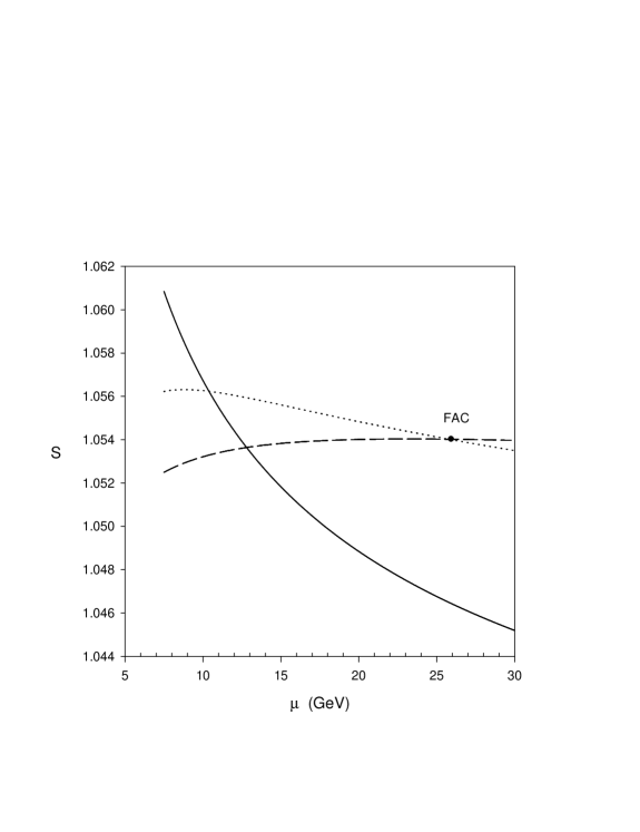
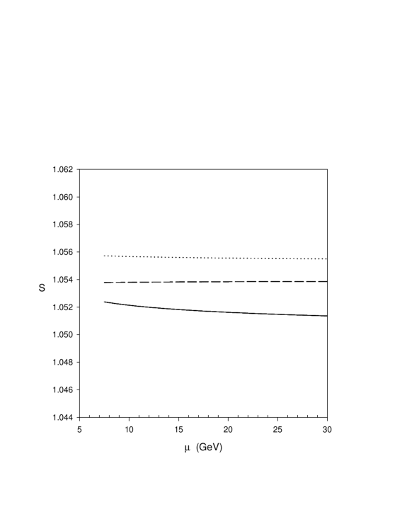
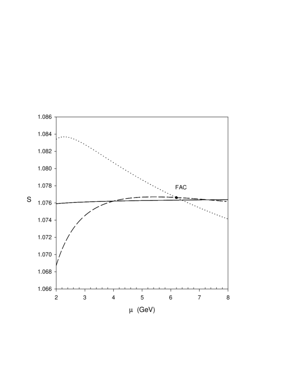
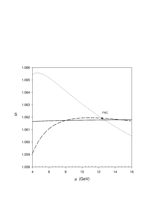
In Figures 7 and 8, we compare the $\mu$-dependence of the unsummed (5.2) and summed (5.6) expressions for $S[x(\mu),\log(\mu^{2}/s)]$, with the choice $s=(15\,{\rm GeV})^{2}$. The running coupling constant $x(\mu)$ is assumed to evolve via the $n_{f}=5$ (four-loop-order) $\beta$-function from an initial value $x(M_{z})=0.11800/\pi$. Although Figure 7 does show a flattening of the unsummed expressions upon incorporation of successively higher orders of perturbation theory $[S^{NL},S^{NNL},S^{N^{3}L}]$, Figure 8 demonstrates that the corresponding RG-summed expressions are order-by-order much less dependent on the renormalization scale $\mu$. In particular, the full $N^{3}L$ summed expression (5.6) exhibits virtually no dependence on $\mu$, but is seen to maintain a constant value $S_{RG\Sigma}^{N^{3}L}=1.05372\pm 0.00004$ over the entire $\sqrt{s}/2\leq\mu\leq 2\sqrt{s}$ range of renormalization scale considered. By contrast the unsummed expression $S^{N^{3}L}$ of (5.2) is seen to increase (modestly) over this same range from 1.0525 to 1.0540. The point marked FAC in Figure 7 is the intersection of the unsummed expressions for $S^{NNL}$ and $S^{N^{3}L}$. This point is the particular choice of $\mu$ at which the ${\cal{O}}(x^{3})$ contribution to (5.2) vanishes, i.e., the point of fastest apparent convergence (FAC). It is noteworthy that this FAC value for $S^{N^{3}L}$ is quite close to the RG-summation value $S_{RG\Sigma}^{N^{3}L}$, a result anticipated by Maxwell [5]. In other words, if one were to use the FAC criterion to reduce the theoretical uncertainty arising from $\mu$-dependence in the original expression (5.2) for $S^{N^{3}L}(\mu)$ over the $\sqrt{s}/2\leq\mu\leq 2\sqrt{s}$ range considered, the specific value one would obtain [$S_{FAC}^{N^{3}L}=S^{N^{3}L}(26\,{\rm GeV})=1.05402$] corresponds very nearly to the RG-summation value extracted from (5.6) [$S_{RG\Sigma}^{N^{3}L}=1.05372\pm 0.00004$].

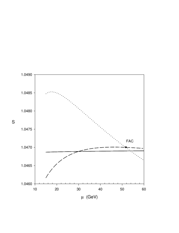
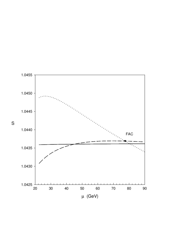
This behaviour is not peculiar to the choice of $s$ in Figs. 7 and 8. In Figures 9 and 10, we consider $S^{N^{2}L}$, $S^{N^{3}L}$ and $S_{RG\Sigma}^{N^{3}L}$ for $\sqrt{s}=30\,{\rm GeV}$ and $\sqrt{s}=45\;\,{\rm GeV}$. The FAC point each figure occurs at the value of $\mu$ for which $S^{NNL}(\mu)=S^{N^{3}L}(\mu)$, as discussed above. In both figures it is evident that $S^{N^{3}L}$ has substantially more variation with $\mu$ than $S_{RG\Sigma}^{N^{3}L}$, which is virtually independent of $\mu$. Nevertheless, both figures also show that the FAC point of $S^{N^{3}L}$ is very close to the $S_{RG\Sigma}^{N^{3}L}$-level value. For $\sqrt{s}=30\,{\rm GeV}$ [Fig.  9] $S_{FAC}^{N^{3}L}=S^{N^{3}L}(\mu=52\,{\rm GeV})=1.04700$ and $S_{RG\Sigma}^{N^{3}L}=1.04689\pm 0.00002$. For $\sqrt{s}=45\,{\rm GeV}$ [Fig.  10], $S_{FAC}^{N^{3}L}=S^{N^{3}L}(\mu=77\,{\rm GeV})=1.04369$, and $S_{RG\Sigma}^{N^{3}L}=1.04360\pm 0.00001$.

Similarly, the PMS points in all three figures, corresponding to maxima of $S^{N^{3}L}(\mu)$, are very near the FAC points and also quite close to the $S_{RG\Sigma}^{N^{3}L}$ level. In Fig. 7 $[\sqrt{s}=15\,{\rm GeV}]$, $S_{PMS}^{N^{3}L}=S^{N^{3}L}(23\,{\rm GeV})=1.05403$; in Fig.  9 $[\sqrt{s}=30\,{\rm GeV}]$, $S_{PMS}^{N^{3}L}=S^{N^{3}L}(46\;\,{\rm GeV})=1.04701$; and in Fig.  10 $[\sqrt{s}=45\,{\rm GeV}]$, $S_{PMS}^{N^{3}L}=S^{N^{3}L}(70\,{\rm GeV})=1.04370$. Of course, equality between $S^{N^{3}L}(\mu)$ and $S_{RG\Sigma}^{N^{3}L}$ is necessarily exact when $L=0$, i.e., when $\mu^{2}$ is chosen equal to $s$. This is indeed the prescription employed in the standard [10] prescription relating $S^{N^{3}L}$ to $R(s)$ [18]:

$$R(s)=1+x\left(\sqrt{s}\right)+T_{2,0}~{}x^{2}\!\left(\sqrt{s}\right)+T_{3,0}~{}x^{3}\!\left(\sqrt{s}\right),$$ (5.10)

where $T_{2,0}$ and $T_{3,0}$ are given in Table 1 for $n_{f}=\{3,4,5\}$. The point here, however, is that this prescription is justified not by the $\mu$-invariance of $S^{N^{3}L}\left[x(\mu),\log\left(\mu^{2}/s\right)\right]$, the truncated perturbative series, but by that of $S_{RG\Sigma}^{N^{3}L}$, the perturbative series incorporating the closed-form summation of all RG-accessible logarithms within higher-order terms. Moreover, the nearly $\mu$-independent result $S_{RG\Sigma}^{N^{3}L}$ appears to be quite close to the result one would obtain from $S^{N^{3}L}\left[x(\mu),\log\left(\mu^{2}/s\right)\right]$ either by imposing FAC or PMS criteria to establish an optimal value of $\mu$, as graphically evident from Figs. 9 and 10. That optimal value for $\mu$, however, is not $\mu=\sqrt{s}$, but a substantially larger value of $\mu$ for each case considered.

These results are not peculiar to the choice $n_{f}=5$. Using the Table 1 entries for the parameters $T_{2,0},\;T_{3,0},\;G,P,U$ and $V$ appearing in (4.7) and (4.8), we find for $n_{f}=3$ that

$$\begin{split}S_{RG\Sigma}^{N^{3}L}[x,L]=1&+\frac{x}{1-\frac{9}{4}xL}+\frac{x^{2}\left[1.63982-\frac{16}{9}\log\left(1-\frac{9}{4}xL\right)\right]+x^{3}\left(-\frac{3397}{2592}\right)}{\left(1-\frac{9}{4}xL\right)^{2}}\\ &+\frac{x^{3}\left[-8.97333-8.99096\log\left(1-\frac{9}{4}xL\right)+\frac{256}{81}\log^{2}\left(1-\frac{9}{4}xL\right)\right]}{\left(1-\frac{9}{4}xL\right)^{3}}\end{split}$$ (5.11)

and for $n_{f}=4$ that

$$\begin{split}S_{RG\Sigma}^{N^{3}L}[x,L]=1&+\frac{x}{1-\frac{25}{12}xL}+\frac{x^{2}\left[1.52453-\frac{77}{50}\log\left(1-\frac{25}{12}xL\right)\right]+x^{3}\left(-\frac{121687}{180000}\right)}{\left(1-\frac{25}{12}xL\right)^{2}}\\ &+\frac{x^{3}\left[-11.0096-7.06715\log\left(1-\frac{25}{12}xL\right)+\frac{5929}{2500}\log^{2}\left(1-\frac{25}{12}xL\right)\right]}{\left(1-\frac{25}{12}xL\right)^{3}}\end{split}$$ (5.12)

In Figures 11 and 12 we display the expression (5.12) for $S_{RG\Sigma}^{N^{3}L}$ together with (unsummed $n_{f}=4$ expressions for) $S^{N^{3}L}$ and $S^{NNL}$ for $\sqrt{s}=4\,{\rm GeV}$ and $\sqrt{s}=8\,{\rm GeV}$. To generate these figures, we evolve $x(\mu)$ using an initial condition $x(4.17\,{\rm GeV})=0.0716218$ [2] appropriate for $n_{f}=4$ and obtained from the threshold matching conditions [21] to the $n_{f}=5$ running couplant $x(4.17\,{\rm GeV})=0.0715492$ evolved from $x\left(M_{Z}\right)=0.118/\pi$ [10]. As in Figs. 9 and 10 we see that $S_{PMS}^{N^{3}L}$ and $S_{FAC}^{N^{3}L}$ are both close to the very-nearly constant $S_{RG\Sigma}^{N^{3}L}$ level, although the PMS and FAC values for $\mu$ are substantially larger than $\sqrt{s}$ in each case.

To conclude, the primary result of interest is that closed-form summation of all RG-accessible logarithms to any given order of perturbation theory leads to expressions (e.g. Fig. 8) that order-by-order are substantially less scale-dependent than the corresponding truncated series (Fig. 7). The scale-independence of $S_{RG\Sigma}^{N^{3}L}$ supports the prescription of choosing $\mu=\sqrt{s}$ in the unsummed series $S^{N^{3}L}\left[\mu^{2},\;\log(\mu^{2}/s)\right]$, since the summed and unsummed series coincide at this value of $\mu$. However, the unsummed series $S^{N^{3}L}$ still exhibits noticeable scale dependence. The use of FAC and PMS criteria to find an optimal value for $\mu$ for $S^{N^{3}L}$ leads to values for this unsummed series which are quite close to its RG-summation value.

6 Other Perturbative Applications

6.1 Momentum Space QCD Static Potential

The momentum space expression for the perturbative portion of the QCD static potential function

$$V(r)=\int\frac{\mathrm{d}^{3}q}{(2\pi)^{3}}\,\mathrm{e}^{\mathrm{i}\vec{q}\cdot\vec{r}}\left(-\frac{16\pi^{2}}{3\vec{q}^{\;2}}\right)W\left[\frac{\alpha_{s}(\mu)}{\pi},\log\left(\frac{\mu^{2}}{\vec{q}^{\;2}}\right)\right]$$ (6.1)

is given by the integrand series

$$W[x,L]=x+\left(T_{2,0}+T_{2,1}L\right)x^{2}+\left(T_{3,0}+T_{3,1}L+T_{3,2}L^{2}\right)x^{3}+\ldots$$ (6.2)

where $x\equiv\alpha_{s}(\mu)/\pi$, $L=\log\left(\mu^{2}/\vec{q}^{\,2}\right)$, and where the series coefficients within (6.2) are [22]

$$\begin{split}T_{2,0}&=31/12-5n_{f}/18,\;\;T_{2,1}=\beta_{0}=11/4-n_{f}/6,\\ T_{3,0}&=28.5468-4.14714n_{f}+25n_{f}^{2}/324,\;T_{3,1}=247/12-229n_{f}/72+5n_{f}^{2}/54,\;\;T_{3,2}=\beta_{0}^{2}.\end{split}$$ (6.3)

The function $W[x,L]$ is shown in [23] to satisfy the same RG equation (5.4) as the semileptonic $b\rightarrow u$ and $b\rightarrow c$ decay rate in the pole mass scheme. Consequently, the closed form summation of all RG-accessible logs is given by eqs. (4.6)–(4.8), with the constants $G,P,U$ and $V$ as given by eqs. (4.1)–(4.4). Since $T_{0,0}$, as defined by the generic series form (1.1), is zero for the series (6.2), the series $S_{0}=\sum_{n=0}^{\infty}T_{n,n}(xL)^{n}$ is trivially zero. Thus, the RG-summation of $W[x,L]$ is

$$W_{RG\Sigma}=xS_{1}[xL]+x^{2}S_{2}[xL]+x^{3}S_{3}[xL].$$ (6.4)

Noting that $T_{1,0}=1$ in (6.2), we find for $n_{f}=\{3,4,5\}$ that

$$\begin{split}W_{RG\Sigma}^{n_{f}=5}=&\frac{x}{(1-\frac{23}{12}xL)}+\frac{x^{2}\left[\frac{43}{36}-\frac{29}{23}\log\left(1-\frac{23}{12}xL\right)\right]+x^{3}\left[\frac{17521}{152352}\right]}{\left(1-\frac{23}{12}xL\right)^{2}}\\ &+\frac{x^{3}\left[9.62511-\frac{43819}{9522}\log\left(1-\frac{23}{12}xL\right)+\frac{841}{529}\log^{2}\left(1-\frac{23}{12}xL\right)\right]}{\left(1-\frac{23}{12}xL\right)^{3}}\end{split}$$ (6.5)

$$\begin{split}W_{RG\Sigma}^{n_{f}=4}=&\frac{x}{(1-\frac{25}{12}xL)}+\frac{x^{2}\left[\frac{53}{36}-\frac{77}{50}\log\left(1-\frac{25}{12}xL\right)\right]-x^{3}\left[\frac{121687}{180000}\right]}{\left(1-\frac{25}{12}xL\right)^{2}}\\ &+\frac{x^{3}\left[13.8688-\frac{77693}{11250}\log\left(1-\frac{25}{12}xL\right)+\frac{5929}{2500}\log^{2}\left(1-\frac{25}{12}xL\right)\right]}{\left(1-\frac{25}{12}xL\right)^{3}}\end{split}$$ (6.6)

$$\begin{split}W_{RG\Sigma}^{n_{f}=3}=&\frac{x}{\left(1-\frac{9}{4}xL\right)}+\frac{x^{2}\left[\frac{7}{4}-\frac{16}{9}\log\left(1-\frac{9}{4}xL\right)\right]-x^{3}\left[\frac{3397}{2592}\right]}{\left(1-\frac{9}{4}xL\right)^{2}}\\ &+\frac{x^{3}\left[18.1104-\frac{760}{81}\log\left(1-\frac{9}{4}xL\right)+\frac{256}{81}\log^{2}\left(1-\frac{9}{4}xL\right)\right]}{\left(1-\frac{9}{4}xL\right)^{3}}\end{split}$$ (6.7)

In Fig. 13 we plot both the truncated series $W^{NNL}[x,L]$, consisting of the terms explicitly appearing in (6.2), as well as the corresponding RG-summed series (6.5) for the $n_{f}=5$ case with $|\vec{q}|=4\,{\rm GeV}$. As before, we determine $x(\mu)$ from eq. (2.3) with the initial condition $\alpha_{s}(4.17\,{\rm GeV})/\pi=0.071549$ devolving from $\alpha_{s}(M_{z})=0.118000$. Although the truncated series varies only modestly [$0.0856\geq W^{NNL}\geq 0.0795$] over the range $|\vec{q}|/2<\mu<2|\vec{q}|$, the RG-summed series is seen to exhibit less than 10% of the unsummed series’ variation over this same range of $\mu$ $[0.08295\geq W_{RG\Sigma}\geq 0.08233]$.

6.2 Gluonic Scalar Correlation Function

The imaginary part of the correlator for gluonic scalar currents

$$j_{G}(y)=\frac{\beta(x(\mu))}{\pi x(\mu)\beta_{0}}G_{\mu\nu}^{a}(y)G^{\mu\nu,a}(y)$$ (6.8)

enters QCD sum rules pertinent to scalar glueball properties [24], and is given by $(s\equiv p^{2},\;x(\mu)=\alpha_{s}(\mu)/\pi)$

$${\rm Im}\Pi_{G}(s)={\rm Im}\left\{\mathrm{i}\int\mathrm{d}^{4}y\;\mathrm{e}^{\mathrm{i}p\cdot y}<0|Tj_{G}(y)j_{G}(0)|0>\right\}=\frac{2x^{2}(\mu)s^{2}}{\pi^{3}}S\left[x(\mu),\;\log\left(\mu^{2}/s\right)\right]$$ (6.9)

where

$$S[x,L]=1+\sum_{n=1}^{\infty}\sum_{m=0}^{n}T_{n,m}x^{n}L^{m}.$$ (6.10)

The leading coefficients $T_{n,m}$ within (6.10) can be extracted from a three-loop calculation by Chetyrkin, Kniehl and Steinhauser [25, 19] and are tabulated in Table 2.

The correlator $Im\Pi_{G}(s)$ is RG-invariant: $\mu^{2}\mathrm{d}Im\Pi_{G}(s)/\mathrm{d}\mu^{2}=0$. Consequently the series (6.10) can be shown to satisfy the RG- equation

$$\left(\frac{\partial}{\partial L}+\beta(x)\frac{\partial}{\partial x}+\frac{2\beta(x)}{x}\right)S[x,L]=0.$$ (6.11)

Upon substituting (6.10) into (6.11), it is straightforward to show that the aggregate coefficients of $x^{n}L^{n-1},\;x^{n}L^{n-2}$ and $x^{n}L^{n-3}$ respectively vanish provided

$$nT_{n,n}-\beta_{0}(n+1)T_{n-1,\;n-1}=0,$$ (6.12)

$$(n-1)T_{n,n-1}-\beta_{0}(n+1)T_{n-1,\;n-2}-\beta_{1}nT_{n-2,\;n-2}=0,$$ (6.13)

$$(n-2)T_{n,n-2}-\beta_{0}(n+1)T_{n-1,\;n-3}-\beta_{1}nT_{n-2,\;n-3}-\beta_{2}(n-1)T_{n-3,\;n-3}=0.$$ (6.14)

We employ the definitions (2.18), (2.19) and (2.20) for $S_{0}$, $S_{1}$ and $S_{2}$. By multiplying (6.12) by $u^{n-1}$, (6.13) by $u^{n-2}$ and (6.14) by $u^{n-3}$ and summing from $n=1,2$ and $3$ respectively, we obtain the following three linear differential equations

$$(1-\beta_{0}u)\frac{\mathrm{d}S_{0}}{\mathrm{d}u}-2\beta_{0}S_{0}=0$$ (6.15)

$$(1-\beta_{0}u)\frac{\mathrm{d}S_{1}}{\mathrm{d}u}-3\beta_{0}S_{1}=\beta_{1}\left[u\frac{\mathrm{d}S_{0}}{\mathrm{d}u}+2S_{0}\right],$$ (6.16)

$$(1-\beta_{0}u)\frac{\mathrm{d}S_{2}}{\mathrm{d}u}-4\beta_{0}S_{2}=\beta_{1}\left[u\frac{\mathrm{d}S_{1}}{\mathrm{d}u}+3S_{1}\right]+\beta_{2}\left[u\frac{\mathrm{d}S_{0}}{\mathrm{d}u}+2S_{0}\right].$$ (6.17)

Given the $u=0$ initial conditions $S_{0}=1,\;S_{1}=T_{1,0},\;S_{2}=T_{2,0}$ and setting $u=xL$, we obtain the following RG-summed version of the series (6.10) to NNL order:

$$\begin{split}S_{RG\Sigma}^{NNL}=&S_{0}[xL]+xS_{1}[xL]+x^{2}S_{2}[xL]\\ =&\frac{1}{(1-\beta_{0}xL)^{2}}+\frac{x\left[T_{1,0}-\frac{2\beta_{1}}{\beta_{0}}\log(1-\beta_{0}xL)\right]+x^{2}\left[\frac{2\beta_{1}^{2}}{\beta_{0}^{2}}-\frac{2\beta_{2}}{\beta_{0}}\right]}{(1-\beta_{0}xL)^{3}}\\ &+x^{2}\frac{\left[\left(T_{2,0}-\frac{2\beta_{1}^{2}}{\beta_{0}^{2}}+\frac{2\beta_{2}}{\beta_{0}}\right)-\left(\frac{3T_{1,0}\beta_{1}}{\beta_{0}}+\frac{2\beta_{1}^{2}}{\beta_{0}^{2}}\right)\log(1-\beta_{0}xL)+(3\beta_{1}^{2}/\beta_{0}^{2})\log^{2}(1-\beta_{0}xL)\right]}{(1-\beta_{0}xL)^{4}}\end{split}$$ (6.18)

where $x=\alpha_{s}(\mu)/\pi$ and $L=\log(\mu^{2}/s)$, as before, and where the $\beta_{k}$ are as defined in (2.3). In Figure 14 we compare the $\mu$-dependence of $x^{2}(\mu)S_{RG\Sigma}^{NNL}$ to that of the corresponding truncated series

$$x^{2}(\mu)S^{NNL}[x,L]=x^{2}\left[1+\left(T_{1,0}+T_{1,1}L\right)x+\left(T_{2,0}+T_{2,1}L+T_{2,2}L^{2}\right)x^{2}\right]$$ (6.19)

for the $n_{f}=3$ case with $\sqrt{s}=2\,{\rm GeV}$. The evolution of $x(\mu)$ is assumed to follow an $n_{f}=3$ $\beta$-function with the initial condition $\alpha_{s}(m_{\tau})/\pi=0.33/\pi$ [17]. As evident from the figure, the severe $\mu$-dependence of $x^{2}S^{NNL}$ is considerably diminished by RG-summation. The RG-summed expression [eq. (6.18) multiplied by $x^{2}(\mu)$] falls from 0.056 to 0.041 as $\mu$ increases from $1\,{\rm GeV}$ to $4\,{\rm GeV}$. By contrast, the unsummed expression (6.19) falls precipitously from 0.259 to 0.017, a factor of 15, over the same range of $\mu$. This unphysical dependence on renormalization scale suggests that $S^{NNL}$ [as in (6.19)] be replaced by (6.18) within sum rule approaches to the lowest-lying scalar gluonium state.

6.3 Cross-Section $\sigma(W_{L}^{+}W_{L}^{-}\rightarrow Z_{L}Z_{L})$

The scattering of two longitudinal $W$’s into two longitudinal $Z$’s is mediated by the Higgs particle of standard-model electroweak physics. Assuming a single Higgs particle (devolving from the single doublet responsible for electroweak symmetry breaking), one finds the cross-section for this process at very high energies $(s>>M_{H}^{2})$ to be

$$\sigma(s)=\frac{8\pi^{2}}{9s}g^{2}(\mu)S[g(\mu),\log\left(\mu^{2}/s\right)],$$ (6.20)

where $g(\mu)=6\lambda_{\overline{\rm{MS}}}(\mu)/16\pi^{2}$, the quartic scalar couplant of the single-doublet standard model, and where the series $S$ is [26]

$$S[g,L]=1+\sum_{n=1}^{\infty}\sum_{m=0}^{n}T_{m,n}g^{n}L^{m}$$ (6.21)

with $g=g(\mu)$,and $L=\log(\mu^{2}/s)$. The constants $T_{n,m}$ are fully known to ${\rm NNL}$ order [26]

$$T_{1,0}=-10.0,\;T_{1,1}=-4,\;T_{2,0}=93.553+\frac{2}{3}\log\left(s/M_{H}^{2}\right),\;T_{2,1}=68.667,\;T_{2,2}=12.$$ (6.22)

The RG-invariance of the physical cross-section $\sigma$ implies that the series $S$ satisfies the RG equation

$$\left(\frac{\partial}{\partial L}+\beta(g)\frac{\partial}{\partial g}+\frac{2\beta(g)}{g}\right)S[g,L]=0$$ (6.23)

This is the same RG-equation as (6.11) characterizing the gluonic scalar correlator, but with the $\beta$-function appropriate for the single-Higgs-doublet $\overline{\rm{MS}}$ quartic scalar couplant $g(\mu)$ [27]:

$$\begin{split}\mu^{2}\frac{\mathrm{d}g}{\mathrm{d}\mu^{2}}&=\beta(g)\equiv-\beta_{0}g^{2}-\beta_{1}g^{3}-\beta_{2}g^{4}\ldots,\\ \beta_{0}&=-2,\;\beta_{1}=\frac{13}{3},\;\beta_{2}=-27.803\end{split}$$ (6.24)

Consequently the RG-summed version of $S$ is given by (6.18):

$$\begin{split}S_{RG\Sigma}=&\frac{1}{(1+2gL)^{2}}+\frac{g\left[-10+\frac{13}{3}\log(1+2gL)\right]-18.4141g^{2}}{(1+2gL)^{3}}\\ &+\frac{g^{2}\left[111.967+\frac{2}{3}\log\left(\frac{s}{M_{H}^{2}}\right)-\frac{1339}{18}\log(1+2gL)+\frac{169}{12}\log^{2}(1+2gL)\right]}{(1+2gL)^{4}}\end{split}$$ (6.25)

6.4 Higgs Decay $H\rightarrow gg$

Higher-order expressions for the decay of a Higgs boson into two gluons have been obtained and studied both outside [28] and within [29, 30, 31] the context of a standard-model single-doublet Higgs field. In the limit $M_{H}^{2}<<4M_{t}^{2},\;\;M_{b}=0$ the latter decay rate is of the form

$$\Gamma=\left[\sqrt{2}G_{F}M_{H}^{3}/72\pi\right]x^{2}(\mu)S\left[x(\mu),\log\left(\mu^{2}/m_{t}^{2}(\mu)\right)\!,\log\left(M_{H}^{2}/M_{t}^{2}\right)\right].$$ (6.26)

Capitalized masses $\left(M_{H},M_{t}\right)$ denote RG-invariant pole masses, whereas $m_{t}(\mu)$ is the running t-quark mass. The series $S$ within (6.26) is of the generic form (1.1) with $L\equiv\log\left(\mu^{2}/m_{t}^{2}(\mu)\right)$, but the coefficients $T_{n,m}$ are now dependent upon the RG-invariant logarithm $T\equiv\log\left(M_{H}^{2}/M_{t}^{2}\right)$. Using six active flavours to accommodate the running of $m_{t}(\mu)$, one can extract from ref. [29] the following two subleading orders of series coefficients within $S$ [30]:

$$\begin{split}T_{0,0}&=1,\;T_{1,0}(T)=\frac{215}{12}-\frac{23}{6}T,\;T_{1,1}=\frac{7}{2},\\ T_{2,0}(T)&=146.8912-\frac{4903}{48}T+\frac{529}{48}T^{2},T_{2,1}(T)=\frac{1445}{16}-\frac{161}{8}T,\;T_{2,2}=\frac{147}{16}\end{split}$$ (6.27)

RG-invariance of the physical decay rate $\left(\mu^{2}d\Gamma/d\mu^{2}=0\right)$ implies the following RG-equation for the series $S[x,L,T]$ within (6.26):

$$\left[\left(1-2\gamma_{m}(x)\right)\frac{\partial}{\partial L}+\beta(x)\frac{\partial}{\partial x}+\frac{2\beta(x)}{x}\right]S[x,L,T]=0.$$ (6.28)

The $n_{f}=6$ values for the $\overline{{\rm MS}}$ $\beta$- and $\gamma_{m}$-functions are

$$\begin{split}\beta(x)&=-\left(\beta_{0}x^{2}+\beta_{1}x^{3}+\beta_{2}x^{4}+\ldots\right),\;\;\beta_{0}=7/4,\beta_{1}=13/8,\beta_{2}=-65/128\\ \gamma_{m}(x)&=-\left(\gamma_{0}x+\gamma_{1}x^{2}+\gamma_{2}x^{3}+\ldots\right),\;\;\gamma_{0}=1,\gamma_{1}=27/8,\gamma_{2}=4.83866.\end{split}$$ (6.29)

Upon substituting the series $S$, as described above, into (6.28), one finds that the net coefficients of $x^{n}L^{n-1},x^{n}L^{n-2}$ and $x^{n}L^{n-3}$ on the left-hand side of (6.28) vanish provided the following recursion relations are respectively upheld:

$$nT_{n,n}-\beta_{0}(n+1)T_{n-1,n-1}=0$$ (6.30)

$$(n-1)T_{n,n-1}+2\gamma_{0}(n-1)T_{n-1,n-1}-\beta_{0}(n+1)T_{n-1,n-2}-\beta_{1}nT_{n-2,n-2}=0$$ (6.31)

$$\begin{split}0=&(n-2)T_{n,n-2}+2\gamma_{0}(n-2)T_{n-1,n-2}+2\gamma_{1}(n-2)T_{n-2,n-2}\\ &-\beta_{0}(n+1)T_{n-1,n-3}-\beta_{1}nT_{n-2,n-3}-\beta_{2}(n-1)T_{n-3,n-3}\quad.\end{split}$$ (6.32)

By multiplying (6.30) by $u^{n-1}$, (6.31) by $u^{n-2}$ and (6.32) by $u^{n-3}$, and by summing each equation from $n=1,2$ and $3$, respectively, we obtain the following linear differential equations for the summations $S_{0}$ (2.18), $S_{1}$ (2.19) and $S_{2}$ (2.20):

$$(1-\beta_{0}u)\frac{\mathrm{d}S_{0}}{\mathrm{d}u}-2\beta_{0}S_{0}=0$$ (6.33)

$$(1-\beta_{0}u)\frac{\mathrm{d}S_{1}}{\mathrm{d}u}-3\beta_{0}S_{1}=\beta_{1}\left(u\frac{\mathrm{d}S_{0}}{\mathrm{d}u}+2S_{0}\right)-2\gamma_{0}\frac{\mathrm{d}S_{0}}{\mathrm{d}u}$$ (6.34)

$$(1-\beta_{0}u)\frac{\mathrm{d}S_{2}}{\mathrm{d}u}-4\beta_{0}S_{2}=\beta_{1}\left(u\frac{\mathrm{d}S_{1}}{\mathrm{d}u}+3S_{1}\right)-2\gamma_{0}\frac{\mathrm{d}S_{1}}{\mathrm{d}u}+\beta_{2}\left(u\frac{\mathrm{d}S_{0}}{\mathrm{d}u}+2S_{0}\right)-2\gamma_{1}\frac{\mathrm{d}S_{0}}{\mathrm{d}u}$$ (6.35)

Given the $u=0$ initial conditions $S_{0}=1$, $S_{1}=T_{1,0}(T)$, $S_{2}=T_{2,0}(T)$, one can solve for $S_{0}[u]$, $S_{1}[u]$ and $S_{2}[u]$. As before, all-orders summation of the RG-accessible logarithms within the series $S[x,L,T]$ is now possible, given the explicit form of $T_{1,0}(T)$ and $T_{2,0}(T)$ in (6.27) and the explicit $\beta$- and $\gamma$-function coefficients in (6.29). We thus find that

$$\begin{split}S_{RG\Sigma}^{NNL}=&S_{0}[xL]+xS_{1}[xL]+x^{2}S_{2}[xL]\\[5.0pt] =&\frac{1}{\left(1-\frac{7}{4}xL\right)^{2}}+\frac{x\left[\frac{215}{12}-\frac{23}{6}T+\frac{15}{7}\log\left(1-\frac{7}{4}xL\right)\right]+\frac{9479}{784}x^{2}}{\left(1-\frac{7}{4}xL\right)^{3}}\\[5.0pt] &+\frac{x^{2}\left[134.801-\frac{4903}{48}T+\frac{529}{48}T^{2}+\left(\frac{21675}{392}-\frac{345}{28}T\right)\log\left(1-\frac{7}{4}xL\right)+\frac{675}{196}\log^{2}\left(1-\frac{7}{4}xL\right)\right]}{\left(1-\frac{7}{4}xL\right)^{4}}\end{split}$$ (6.36)

6.5 Fermionic Scalar Correlation Function

The imaginary part of the RG-invariant correlator for the fermionic scalar current

$$j_{s}(y)=m\overline{\Psi}(y)\Psi(y)$$ (6.37)

is

$${\rm Im}\;\Pi(s)={\rm Im}\left[\mathrm{i}\int\mathrm{d}^{4}y\;\mathrm{e}^{\mathrm{i}p\cdot y}<0|Tj_{s}(y)j_{s}(0)|0>\right]=\frac{3s}{8\pi}m^{2}(\mu)S\left[x(\mu),\;\log\left(\mu^{2}/s\right)\right],$$ (6.38)

where the series $S[x,L]$ is of the form (1.1) and has been fully calculated to $N^{3}L$ order [32]. For $n_{f}=\{3,4,5\}$ the series coefficients $T_{n,m}$ are tabulated for $(n,m)\leq 3$ in Table 3. This correlation function is relevant both for QCD sum-rule analyses of scalar mesons, a topic of past and present interest [33], and for the decay of a single-doublet standard-model Higgs boson into a $b\bar{b}$ pair [32, 30]. RG-invariance of the correlator ($\mu^{2}\mathrm{d}{\rm Im}\Pi(s)/\mathrm{d}\mu^{2}=0$) implies the following RG-equation for the series $S[x,L]$ within (6.38) [19]:

$$\left[\frac{\partial}{\partial L}+\beta(x)\frac{\partial}{\partial x}+2\gamma_{m}(x)\right]S[x,L]=0,$$ (6.39)

where $L=\log\left(\mu^{2}/s\right)$, $x=\alpha_{s}(\mu)/\pi$, $\beta(x)$ is the $\beta$-function series (2.3) and $\gamma_{m}(x)$ is the $\gamma$-function series (1.3). Substitution of (1.1) into (6.39) leads to the following recursion formulae for the elimination of terms proportional to $x^{n}L^{n-1}$, $x^{n}L^{n-2}$, $x^{n}L^{n-3}$, and $x^{n}L^{n-4}$:

$$0=nT_{n,n}-\beta_{0}(n-1)T_{n-1,n-1}-2\gamma_{0}T_{n-1,n-1}$$ (6.40)

$$0=(n-1)T_{n,n-1}-\beta_{0}(n-1)T_{n-1,n-2}-\beta_{1}(n-2)T_{n-2,n-2}-2\gamma_{0}T_{n-1,n-2}-2\gamma_{1}T_{n-2,n-2}$$ (6.41)

$$\begin{split}0=&(n-2)T_{n,n-2}-\beta_{0}(n-1)T_{n-1,n-3}-\beta_{1}(n-2)T_{n-2,n-3}-\beta_{2}(n-3)T_{n-3,n-3}\\ &-2\gamma_{0}T_{n-1,n-3}-2\gamma_{1}T_{n-2,n-3}-2\gamma_{2}T_{n-3,n-3}\end{split}$$ (6.42)

$$\begin{split}0=&(n-3)T_{n,n-3}-\beta_{0}(n-1)T_{n-1,n-4}-\beta_{1}(n-2)T_{n-2,n-4}-\beta_{2}(n-3)T_{n-3,n-4}\\ &-\beta_{3}(n-4)T_{n-4,n-4}-2\gamma_{0}T_{n-1,n-4}-2\gamma_{1}T_{n-2,n-4}-2\gamma_{2}T_{n-3,n-4}-2\gamma_{3}T_{n-4,n-4}\end{split}$$ (6.43)

We follow the usual procedure of

1. multiplying (6.40) by $u^{n-1}$ and summing from $n=1$ to $\infty$,

2. multiplying (6.41) by $u^{n-2}$ and summing from $n=2$ to $\infty$,

3. multiplying (6.42) by $u^{n-3}$ and summing from $n=3$ to $\infty$, and

4. multiplying (6.43) by $u^{n-4}$ and summing from $n=4$ to $\infty$.

Using the definitions (2.18), (2.19), (2.20) and (2.30) for $\{S_{0},S_{1},S_{2},S_{3}\}$, we then obtain the following four linear differential equations for these summations:

$$(1-\beta_{0}u)\frac{\mathrm{d}S_{0}}{\mathrm{d}u}-2\gamma_{0}S_{0}=0,\;\;S_{0}[0]=1$$ (6.44)

$$(1-\beta_{0}u)\frac{\mathrm{d}S_{1}}{\mathrm{d}u}-(\beta_{0}+2\gamma_{0})S_{1}=\beta_{1}u\frac{\mathrm{d}S_{0}}{\mathrm{d}u}+2\gamma_{1}S_{0},\;\;S_{1}[0]=T_{1,0}$$ (6.45)

$$(1-\beta_{0}u)\frac{\mathrm{d}S_{2}}{\mathrm{d}u}-(2\beta_{0}+2\gamma_{0})S_{2}=\beta_{1}u\frac{\mathrm{d}S_{1}}{\mathrm{d}u}+\beta_{2}u\frac{\mathrm{d}S_{0}}{\mathrm{d}u}+(\beta_{1}+2\gamma_{1})S_{1}+2\gamma_{2}S_{0},\;\;S_{2}[0]=T_{2,0}$$ (6.46)

$$\begin{split}(1-\beta_{0}u)\frac{\mathrm{d}S_{3}}{\mathrm{d}u}-(3\beta_{0}+2\gamma_{0})S_{3}=&\beta_{1}u\frac{\mathrm{d}S_{2}}{\mathrm{d}u}+\beta_{2}u\frac{\mathrm{d}S_{1}}{\mathrm{d}u}+\beta_{3}u\frac{\mathrm{d}S_{0}}{\mathrm{d}u}+(2\beta_{1}+2\gamma_{1})S_{2}\\ &+(\beta_{2}+2\gamma_{2})S_{1}+2\gamma_{3}S_{0},\;\;S_{3}[0]=T_{3,0}\end{split}$$ (6.47)

The solutions to these equations are

$$S_{0}[u]=(1-\beta_{0}u)^{-A}$$ (6.48)

$$S_{1}[u]=C_{1}(1-\beta_{0}u)^{-A}+\frac{[T_{1,0}-C_{1}+C_{2}\log(1-\beta_{0}u)]}{(1-\beta_{0}u)^{A+1}}$$ (6.49)

$$\begin{split}S_{2}[u]=&\frac{D_{1}}{2}(1-\beta_{0}u)^{-A}+\frac{[D_{2}-D_{3}+D_{3}\log(1-\beta_{0}u)]}{(1-\beta_{0}u)^{A+1}}\\ &+\frac{[T_{2,0}-\frac{D_{1}}{2}-D_{2}+D_{3}+D_{4}\log(1-\beta_{0}u)+\frac{D_{5}}{2}\log^{2}(1-\beta_{0}u)]}{(1-\beta_{0}u)^{A+2}}\end{split}$$ (6.50)

$$\begin{split}S_{3}[u]=&\frac{F_{1}}{3}(1-\beta_{0}u)^{-A}+\frac{[\frac{F_{2}}{2}-\frac{F_{3}}{4}+\frac{F_{3}}{2}\log(1-\beta_{0}u)]}{(1-\beta_{0}u)^{A+1}}\\ &+\frac{F_{4}-F_{5}+2F_{6}+(F_{5}-2F_{6})\log(1-\beta_{0}u)+F_{6}\log^{2}(1-\beta_{0}u)]}{(1-\beta_{0}u)^{A+2}}\\ &+\frac{\left[T_{3,0}-\frac{F_{1}}{3}-\frac{F_{2}}{2}+\frac{F_{3}}{4}-F_{4}+F_{5}-2F_{6}+F_{7}\log(1-\beta_{0}u)+\frac{F_{8}}{2}\log^{2}(1-\beta_{0}u)+\frac{F_{9}}{3}\log^{3}(1-\beta_{0}u)\right]}{(1-\beta_{0}u)^{A+3}},\end{split}$$ (6.51)

where

$$A=2\gamma_{0}\beta_{0}$$ (6.52)

$$C_{1}=2\beta_{1}\gamma_{0}/\beta_{0}^{2}-2\gamma_{1}/\beta_{0}$$ (6.53)

$$C_{2}=-2\beta_{1}\gamma_{0}/\beta_{0}^{2}$$ (6.54)

$$D_{1}=\left[C_{1}\left(A\beta_{1}-\beta_{1}-2\gamma_{1}\right)+A\beta_{2}-2\gamma_{2}\right]/\beta_{0}$$ (6.55)

$$D_{2}=\left[C_{1}\left(2\gamma_{1}-2A\beta_{1}\right)-C_{2}\beta_{1}-A\beta_{2}+T_{1,0}\left(A\beta_{1}-2\gamma_{1}\right)\right]/\beta_{0}$$ (6.56)

$$D_{3}=C_{2}\left(A\beta_{1}-2\gamma_{1}\right)/\beta_{0}$$ (6.57)

$$D_{4}=\beta_{1}\left[C_{2}-(A+1)\left(T_{1,0}-C_{1}\right)\right]/\beta_{0}$$ (6.58)

$$D_{5}=-C_{2}\beta_{1}(A+1)/\beta_{0}$$ (6.59)

$$F_{1}=\left[C_{1}\left(A\beta_{2}-2\gamma_{2}-\beta_{2}\right)+D_{1}\left(A\beta_{1}/2-\gamma_{1}-\beta_{1}\right)+A\beta_{3}-2\gamma_{3}\right]/\beta_{0}$$ (6.60)

$$\begin{split}F_{2}=&\frac{1}{\beta_{0}}\biggl{[}D_{3}\left(2\gamma_{1}-A\beta_{1}\right)+D_{2}\left(A\beta_{1}-\beta_{1}-2\gamma_{1}\right)-\frac{D_{1}}{2}A\beta_{1}-C_{2}\beta_{2}\biggr{.}\\ &\qquad\biggl{.}+C_{1}\left(2\gamma_{2}-2A\beta_{2}\right)+T_{1,0}\left(A\beta_{2}-2\gamma_{2}\right)-A\beta_{3}\biggr{]}\end{split}$$ (6.61)

$$F_{3}=\left[D_{3}\left(A\beta_{1}-\beta_{1}-2\gamma_{1}\right)+C_{2}\left(A\beta_{2}-2\gamma_{2}\right)\right]/\beta_{0}$$ (6.62)

$$\begin{split}F_{4}=&\frac{1}{\beta_{0}}\biggl{[}\left(T_{2,0}-D_{1}/2-D_{2}+D_{3}\right)\left(A\beta_{1}-2\gamma_{1}\right)-D_{4}\beta_{1}+D_{3}(A+2)\beta_{1}-D_{2}(A+1)\beta_{1}\biggr{.}\\ &\qquad\biggl{.}+C_{2}\beta_{2}+C_{1}(A+1)\beta_{2}-T_{1,0}(A+1)\beta_{2}\biggr{]}\end{split}$$ (6.63)

$$F_{5}=\left[D_{4}\left(A\beta_{1}-2\gamma_{1}\right)-D_{3}(A+1)\beta_{1}-D_{5}\beta_{1}-C_{2}(A+1)\beta_{2}\right]/\beta_{0}$$ (6.64)

$$F_{6}=D_{5}\left(A\beta_{1}/2-\gamma_{1}\right)/\beta_{0}$$ (6.65)

$$F_{7}=\beta_{1}\left[D_{4}-(A+2)\left(T_{2,0}-D_{1}/2-D_{2}+D_{3}\right)\right]/\beta_{0}$$ (6.66)

$$F_{8}=\beta_{1}\left[D_{5}-D_{4}(A+2)\right]/\beta_{0}$$ (6.67)

$$F_{9}=-\beta_{1}D_{5}(A+2)/\left(2\beta_{0}\right)$$ (6.68)

The ${\cal{O}}(N^{3}L)$ RG-summation of the series $S[x(\mu),\;\log(\mu^{2}/s)]$ appearing in the correlator (6.38) is then found to be

$$\begin{split}S_{RG\Sigma}^{N^{3}L}=&S_{0}\left[x(\mu)\log\left(\frac{\mu^{2}}{s}\right)\right]+x(\mu)S_{1}\left[x(\mu)\log\left(\frac{\mu^{2}}{s}\right)\right]\\ &+x^{2}(\mu)S_{2}\left[x(\mu)\log\left(\frac{\mu^{2}}{s}\right)\right]+x^{3}(\mu)S_{3}\left[x(\mu)\log\left(\frac{\mu^{2}}{s}\right)\right]\end{split}$$ (6.69)

where the RG-summations $S_{0},S_{1},S_{2}$ and $S_{3}$ are given by (6.48)–(6.51) with $u=x(\mu)\log(\mu^{2}/s)$.

In Figure 15 we compare the $\mu$-dependence of the RG-summed scalar fermionic-current correlator,

$${\rm Im}\Pi_{RG\Sigma}^{N^{3}L}\sim m^{2}(\mu)S_{RG\Sigma}^{N^{3}L}$$ (6.70)

to that of the correlator (6.38) when truncated after its fully-known ${\cal{O}}(x^{3})$ contributions,

$${\rm Im}\Pi^{N^{3}L}\sim m^{2}(\mu)\sum_{n=0}^{3}\sum_{m=0}^{n}T_{n,m}x^{n}(\mu)\left[\log\left(\frac{\mu^{2}}{s}\right)\right]^{m},$$ (6.71)

over the range $\sqrt{s}/2\leq\mu\leq 2\sqrt{s}$ with $\sqrt{s}=2\;\,{\rm GeV}$. The coefficients $T_{n,m}$ appearing in (6.71) are given in Table 3. We choose to work in the $\sqrt{s}=2\,{\rm GeV}\;\;n_{f}=3$ regime appropriate for QCD sum rule applications, where the couplant $x(\mu)$ is large. The evolution of $x(\mu)$ is assumed to proceed via the $n_{f}=3$ four-loop $\beta$-function with initial condition $x(m_{\tau})=0.33/\pi$ [17]. The running mass $m(\mu)$ is normalized to $1\;\,{\rm GeV}$ at $\mu=m_{\tau}$ to facilitate comparison of (6.70) to (6.71). In Figure 15, the unsummed correlator is seen to achieve a sharp maximum near $1.5\,{\rm GeV}$, followed by a precipitous fall as $\mu$ approaches $1\,{\rm GeV}$ from above. By contrast, the RG-summed correlator exhibits a much flatter profile, falling from $1.88\,{\rm GeV}^{2}$ to $1.75\,{\rm GeV}^{2}$ as $\mu$ increases from $1$ to $4\,{\rm GeV}$. As in Section 6.2 for the gluonic scalar-current correlator, these results indicate that even $N^{3}L$-order expressions for the perturbative contribution to QCD correlation functions exhibit substantial $\mu$-dependence. Such dependence, which we have shown to be largely eliminated via the RG-summation process, would otherwise percolate through QCD sum-rule integrals as spurious sensitivity on the theory side to the Borel parameter. The incorporation of RG-summed correlators within QCD sum-rule extractions of lowest-lying scalar resonances is currently under investigation.

7 Summary

In this paper we have explicitly summed all RG-accessible logarithms within a number of perturbative processes known to at least two nonleading orders, a procedure originally advocated by Maxwell [5]. As anticipated, we have found the dependence on the renormalization scale $\mu$ in every case examined to be considerably diminished over that of the original series’ known terms.

In semileptonic $b\rightarrow u$ decays in the fully $\overline{\rm{MS}}$ scheme (Section 3), we observe the intriguing possibility that PMS/FAC criteria for the unsummed series truncated to a given order may anticipate the RG-summed series for the next order of perturbation theory. This behaviour, however, is not evident in the other processes we consider. For the vector correlation function (Section 5), PMS/FAC criteria for the unsummed series truncated to a given order coincide closely with the RG-summed series for that same order, but do not anticipate the level of the next-order RG-summation. In the pole-mass scheme version of semi-leptonic B-decays (Section 4), PMS and FAC criteria do not appear applicable to the unsummed series, which monotonically increase with the renormalization scale $\mu$. Indeed, one of the virtues of RG-summation is the sensible scale-independent results it provides for inclusive semileptonic B-decays in the pole mass scheme, a scheme whose unsummed expressions for $b\rightarrow u$ are already known to be problematical [1].

The $\mu$-independence of RG-summation, particularly for the vector-current correlation function (Section 5), is seen to justify the prescription of zeroing all logarithms by setting the renormalization scale to $\mu^{2}$ equal to the kinematic variable $s$. This prescription necessarily equates the unsummed and RG-summed series, and, since the RG-summed series is virtually independent of $\mu$, the zeroing of logarithms in the unsummed series equilibrates it to the flat RG-summation level we obtain.

In Section 6, RG-summation is also applied to the perturbative contributions to the momentum-space QCD static potential, the decay-rate of a standard-model Higgs to two gluons, the Higgs-mediated cross-section $\sigma(WW\rightarrow ZZ)$, and to two scalar-current correlation functions. Examination of these last two quantities in the low-$s$ region appropriate for QCD sum-rules suggests the utility of RG-summation is reducing the unphysical scale-dependence of the perturbative QCD contributions to the field-theoretical side of sum-rules in these channels.

8 Acknowledgements

We are grateful for research support from Leadership Mt. Allison, the International Collaboration Programme 2001 of Enterprise Ireland, 2001 Faculty Summer Grant from SUNY Institute of Technology, and the International Opportunity Fund of the Natural Sciences and Engineering Research Council of Canada. We also acknowledge the hospitality of the High Energy Theory Group at KEK, Tsukuba, Japan, where this research was initiated. Finally, we are grateful to Audrey Kager for valuable contributions to the preparation of this research in manuscript form.

Appendix: An Alternative Closed-Form Summation Procedure

The body of our paper has addressed the evaluation of $S_{n}\left[xL\right]=\sum_{k=0}^{\infty}T_{n+k,k}\left(xL\right)^{k}$, where the full perturbative series $S(x,L)=\sum_{n=0}^{\infty}S_{n}\left[xL\right]x^{n}$. It is, however, also possible to group the terms within $S(x,L)$, as defined by eq. (1.1), such that the dependence of each series term on $x$ and $L$ fully factorises:

$$S(x,L)=\sum_{n=0}^{\infty}R_{n}(x)L^{n}\quad,$$ (A.1)

$$R_{n}(x)=\sum_{k=n}^{\infty}T_{k,n}x^{k}\quad.$$ (A.2)

Let us suppose, for example, that the series $S(x,L)$ satisfies the RGE (2.2) appropriate to $b$-decays. By substituting (A.1) into (2.2), we find that

$$R_{n+1}(x)=\frac{1}{n+1}\left[\frac{1}{2\gamma(x)-1}\right]\left[\beta(x)\frac{\mathrm{d}}{\mathrm{d}x}+5\gamma(x)\right]R_{n}(x)\quad,$$ (A.3)

where we have relabeled the anomalous mass dimension $\gamma_{m}(x)\to\gamma(x)$ to avoid any misinterpretation of the label $m$ as a subscript. If

$$R_{n}(x)\equiv\exp{\left(-\int\limits^{x}\frac{5\gamma\left(x^{\prime}\right)}{\beta\left(x^{\prime}\right)}\,\mathrm{d}x^{\prime}\right)}P_{n}(x)\quad,$$ (A.4)

then the recursion relation (A.3) implies that

$$P_{n+1}(x)=\frac{1}{n+1}\left(\frac{\beta(x)}{2\gamma(x)-1}\right)\frac{\mathrm{d}}{\mathrm{d}x}P_{n}(x)\quad.$$ (A.5)

If one defines $x$ to be implicitly a function of $y$ via the equation

$$\frac{\mathrm{d}}{\mathrm{d}y}x(y)=\frac{\beta(x)}{2\gamma(x)-1}\quad,$$ (A.6)

then (A.5) simplifies to

$$P_{n+1}\left(x(y)\right)=\frac{1}{n+1}\frac{\mathrm{d}}{\mathrm{d}y}P_{n}\left(x(y)\right)\quad,$$ (A.7)

in which case

$$\sum_{n=0}^{\infty}P_{n}\left(x(y)\right)L^{n}=\sum_{n=0}^{\infty}\left(\frac{1}{n!}L^{n}\frac{\mathrm{d}^{n}}{\mathrm{d}y^{n}}\right)P_{0}\left(x(y)\right)=P_{0}\left(x(y+L)\right)\quad.$$ (A.8)

This last result implies via (A.4) that the series $S(x,L)$ is fully determined by knowledge of the log-free summation $R_{0}$, i.e. that

$$S(x,L)=\exp{\left[\int\limits_{x(y)}^{x(y+L)}\frac{5\gamma\left(x^{\prime}\right)}{\beta\left(x^{\prime}\right)}\,\mathrm{d}x^{\prime}\right]}R_{0}\left(x(y+L)\right)$$ (A.9)

where $x(y)$ is defined implicitly by the constraint

$$y=\int\limits^{x}\frac{2\gamma\left(x^{\prime}\right)-1}{\beta\left(x^{\prime}\right)}\,\mathrm{d}x^{\prime}$$ (A.10)

obtained by integrating (A.6).

Using lowest-order expressions $\beta(x)=-\beta_{0}x^{2}$ and $\gamma(x)=-\gamma_{0}x$, we find from (A.10) that

$$y=\frac{1}{\beta_{0}}\left(-\frac{1}{x}+2\gamma_{0}\log(x)\right)+K\quad.$$ (A.11)

If we set

$$x=\frac{1}{2\gamma_{0}W}\quad,\quad K=\frac{2\gamma_{0}}{\beta_{0}}\log{\left(2\gamma_{0}\right)}$$ (A.12)

we find from (A.11) that

$$W\mathrm{e}^{W}=\exp{\left(-\frac{\beta_{0}y}{2\gamma_{0}}\right)}\quad.$$ (A.13)

Eq. (A.13) is the defining relationship for the Lambert $W$-function $W\left[\exp{\left(-\beta_{0}y/2\gamma_{0}\right)}\right]$, as discussed in ref. [36]. Since

$$x(y)=\frac{1}{2\gamma_{0}W\left[\exp{\left(-\beta_{0}y/2\gamma_{0}\right)}\right]}$$ (A.14)

in the approximation $\beta(x)\cong-\beta_{0}x^{2}$, $\gamma(x)\cong-\gamma_{0}x$, we then find from (A.9) that

$$S(x,L)=\left[\frac{W\left[\exp{\left(-\beta_{0}y/2\gamma_{0}\right)}\right]}{W\left[\exp{\left(-\beta_{0}(y+L)/2\gamma_{0}\right)}\right]}\right]^{5\gamma_{0}/\beta_{0}}R_{0}\left(\frac{1}{2\gamma_{0}W\left[\exp{\left(-\beta_{0}(y+L)/2\gamma_{0}\right)}\right]}\right)\quad,$$ (A.15)

where

$$R_{0}(x)=\sum_{k=0}^{\infty}T_{k,0}x^{k}=S(x,0)$$ (A.16)

and where

$$y=-\frac{1}{\beta_{0}x}+\frac{2\gamma_{0}}{\beta_{0}}\log\left(2\gamma_{0}x\right)\quad.$$ (A.17)

For the RGE (4.16), corresponding to (2.2) with $\gamma_{m}(x)$ chosen to be zero, the solution (A.9) still applies provided $x(y)$ is defined implicitly via the constraint

$$y=-\int\limits^{x}\frac{\mathrm{d}x^{\prime}}{\beta\left(x^{\prime}\right)}\quad.$$ (A.18)

In the approximation $\beta(x)=-\beta_{0}x^{2}$, one can choose

$$x(y)\equiv-\frac{1}{\beta_{0}y}$$ (A.19)

in which case

$$S(x,L)=R_{0}\left(\frac{x}{1-\beta_{0}Lx}\right)\quad,$$ (A.20)

where the function $R_{0}$ is as defined via (A.16).

	$n_{f}=3$	$n_{f}=4$	$n_{f}=5$
$\beta_{0}$	9/4	25/12	23/12
$\beta_{1}$	4	77/24	29/12
$\beta_{2}$	3863/384	21943/3456	9769/3456
$T_{2,0}$	1.63982	1.52453	1.40924
$T_{2,1}$	9/4	25/12	23/12
$T_{3,0}$	-10.2839	-11.6856	-12.8046
$T_{3,1}$	11.3792	9.56054	7.81875
$T_{3,2}$	81/16	625/144	529/144
$G$	-16/9	-77/50	-29/23
$P$	$-\frac{3397}{2592}$	$-\frac{121687}{180000}$	$\frac{17521}{152352}$
$U$	-8.99096	-7.06715	-5.14353
$V$	512/81	5929/1250	1682/529

Table 1: Constants for determining the ${\cal{O}}(N^{3}L)$ RG-summation of the $N^{3}L$-order vector-current correlation function.

	$n_{f}=2$	$n_{f}=3$	$n_{f}=4$	$n_{f}=5$	$n_{f}=6$
$T_{1,0}$	$\frac{6919}{348}$	$\frac{659}{36}$	$\frac{4999}{300}$	$\frac{4123}{276}$	$\frac{367}{28}$
$T_{1,1}$	$\frac{29}{6}$	$\frac{9}{2}$	$\frac{25}{6}$	$\frac{23}{6}$	$\frac{7}{2}$
$T_{2,0}$	246.434	197.515	150.210	104.499	60.3685
$T_{2,1}$	$\frac{7379}{48}$	$\frac{2105}{16}$	$\frac{1769}{16}$	$\frac{4355}{48}$	$\frac{1153}{16}$
$T_{2,2}$	$\frac{841}{48}$	$\frac{243}{16}$	$\frac{625}{48}$	$\frac{529}{48}$	$\frac{147}{16}$

Table 2: ${\rm NNL}$-order series coefficients within the gluonic scalar current correlation function.

	$n_{f}=3$	$n_{f}=4$	$n_{f}=5$
$T_{0,0}$	1	1	1
$T_{1,0}$	17/3	17/3	17/3
$T_{1,1}$	2	2	2
$T_{2,0}$	31.8640	30.5054	29.1467
$T_{2,1}$	95/3	274/9	263/9
$T_{2,2}$	17/4	49/12	47/12
$T_{3,0}$	89.1564	65.1980	41.7576
$T_{3,1}$	297.596	267.589	238.381
$T_{3,2}$	229/2	22547/216	10225/108
$T_{3,3}$	221/24	1813/216	1645/216
$\beta_{3}$	47.2280	31.3874	18.8522
$\gamma_{3}$	44.2628	27.3028	11.0343

Table 3: $N^{3}L$-order series coefficients within the fermionic scalar current correlation function, as calculated in [32]. Also listed are the four-loop $\beta$-function [34] and $\gamma$-function [35] coefficients $\beta_{3}$ and $\gamma_{3}$ required for the evaluation of the series $S_{3}$.

Figure 1: Comparison of the next-to-next-to-leading- (NNL-) order unsummed (dotted line) and RG-summed (solid line) decay rates $\Gamma/{\cal K}$ for $b\to u\ell^{-}\bar{\nu}_{\ell}$ in the fully-$\overline{{\rm MS}}$ scheme with five active flavours ($n_{f}=5$). The quantity ${\cal K}\equiv G_{F}^{2}\left|V_{ub}\right|^{2}/192\pi^{3}$.

Figure 2: Comparison of unsummed $b\to u\ell^{-}\bar{\nu}_{\ell}$ decay rates in the fully-$\overline{{\rm MS}}$ scheme ($n_{f}=5$) truncated after NL-order (solid line), NNL-order (dotted line), and ${\rm N^{3}L}$-order (dashed line).

Figure 3: Comparison of RG-summation expressions for the fully-$\overline{{\rm MS}}$ $b\to u\ell^{-}\bar{\nu}_{\ell}$ decay rate ($n_{f}=5$) obtained from the NL (solid line), NNL (dotted line) and ${\rm N^{3}L}$ (dashed line) perturbative series.

Figure 4: Comparison of the large-$\mu$ behaviour of the NNL unsummed (dotted line) and RG-summed (solid line) decay rates for $b\to u\ell^{-}\bar{\nu}_{\ell}$ within the RG-invariant pole-mass scheme with five active flavours.

Figure 5: Comparison of the NNL unsummed (dotted line) and RG-summed (solid line) decay rates for $b\to u\ell^{-}\bar{\nu}_{\ell}$ ($n_{f}=5$) within the pole-mass scheme over the range $m_{b}^{pole}/2\lesssim\mu\lesssim 2m_{b}^{pole}$.

Figure 6: Comparison of unsummed and RG-summed $b\to c\ell^{-}\bar{\nu}_{\ell}$ decay rates $\Gamma/{\cal K}$ ($n_{f}=4$) in the pole-mass scheme, where ${\cal K}\equiv G_{F}^{2}\left|V_{cb}\right|^{2}/192\pi^{3}$. The curves representing the unsummed rates are labelled by NL, NNL and ${\rm N^{3}L}$ indicating the order at which they are truncated. Similiarly, the RG-summed curves are labelled by $\Sigma{\rm NL}$, $\Sigma{\rm N^{2}L}$ and $\Sigma{\rm N^{3}L}$.

Figure 7: Comparison of the following $n_{f}=5$ vector-current correlation-function series when $\sqrt{s}=15\,{\rm GeV}$: $S^{NL}$ (solid line), the $\overline{{\rm MS}}$ perturbative series $S\left[x(\mu),\log\left(\mu^{2}/s\right)\right]$ truncated after NL-order contributions; $S^{NNL}$ (dotted line), the same series truncated after NNL-order contributions; and $S^{N^{3}L}$ (dashed line), the same series truncated after ${\rm N^{3}L}$-order contributions. At the intersection of $S^{NNL}$ with $S^{N^{3}L}$, the ${\rm N^{3}L}$-order contribution to the perturbative series is zero, corresponding to the point of fastest apparent convergence (FAC).

Figure 8: Comparison of the following RG-summations of the perturbative $\overline{{\rm MS}}$ series within the $n_{f}=5$ vector-current correlation-function when $\sqrt{s}=15\,{\rm GeV}$: $S_{RG\Sigma}^{NL}$ (solid line), the summation based upon the perturbative series $S\left[x(\mu),\log\left(\mu^{2}/s\right)\right]$ truncated after NL-order contributions; $S_{RG\Sigma}^{NNL}$ (dotted line), the summation based upon the perturbative series truncated after NNL-order contributions; and $S_{RG\Sigma}^{N^{3}L}$ (dashed line), the summation based upon the perturbative series truncated after ${\rm N^{3}L}$-order contributions.

Figure 9: Comparison of $S^{NNL}$ (dotted line), $S^{N^{3}L}$ (dashed line), and $S_{RG\Sigma}^{N^{3}L}$ (solid line) expressions for the series $S\left[x(\mu),\log\left(\mu^{2}/s\right)\right]$ within the $n_{f}=5$ vector-current correlation-function when $\sqrt{s}=30\,{\rm GeV}$.

Figure 10: Comparison of $S^{NNL}$ (dotted line), $S^{N^{3}L}$ (dashed line), and $S_{RG\Sigma}^{N^{3}L}$ (solid line) expressions for the series $S\left[x(\mu),\log\left(\mu^{2}/s\right)\right]$ within the $n_{f}=5$ vector-current correlation-function when $\sqrt{s}=45\,{\rm GeV}$.

Figure 11: Comparison of $S^{NNL}$ (dotted line), $S^{N^{3}L}$ (dashed line), and $S_{RG\Sigma}^{N^{3}L}$ (solid line) expressions for the series $S\left[x(\mu),\log\left(\mu^{2}/s\right)\right]$ within the $n_{f}=4$ vector-current correlation-function when $\sqrt{s}=4\,{\rm GeV}$.

Figure 12: Comparison of $S^{NNL}$ (dotted line), $S^{N^{3}L}$ (dashed line), and $S_{RG\Sigma}^{N^{3}L}$ (solid line) expressions for the series $S\left[x(\mu),\log\left(\mu^{2}/s\right)\right]$ within the $n_{f}=4$ vector-current correlation-function when $\sqrt{s}=8\,{\rm GeV}$.

Figure 13: The momentum-space $n_{f}=5$ static-potential function series $W^{NNL}$ (dotted line), and the corresponding RG-summation $W^{NNL}_{RG\Sigma}$ (solid line) with $\left|\vec{q}\right|=4\,{\rm GeV}$.

Figure 14: The imaginary part of the gluonic scalar-current correlation function (6.9), as obtained from $x^{2}(\mu)\,S^{NNL}$ (dotted line) and from $x^{2}(\mu)\,S^{NNL}_{RG\Sigma}$ (solid line) with $n_{f}=3$ and $\sqrt{s}=2\,{\rm GeV}$.

Figure 15: The imaginary part of the fermionic scalar-current correlation function (6.38), as obtained from $m^{2}(\mu)\,S^{NNL}$ (dotted line) and from $m^{2}(\mu)\,S^{NNL}_{RG\Sigma}$ (solid line) with $n_{f}=3$ and $\sqrt{s}=2\,{\rm GeV}$.

References

• [1] T. van Ritbergen, Phys. Lett. B 454 (1999) 353;
T. Seidensticker and M. Steinhauser, Phys. Lett.  B 467 (1999) 271.
• [2] M.R. Ahmady, F.A. Chishtie, V. Elias and T.G. Steele, Phys. Lett. B 479 (2000) 201.
• [3] M.R. Ahmady, F.A. Chishtie, V. Elias, A.H. Fariborz, D.G.C. McKeon, T.N. Sherry and T.G. Steele, to appear J. Phys. G (hep-ph/0201236).
• [4] G. ’tHooft, Nucl. Phys. B 61 (1973) 455;
J.C. Collins and A.J. Macfarlane, Phys. Rev. D 10 (1974) 1201.
• [5] C.J. Maxwell, Nucl. Phys. B Proc. Suppl. 86 (2000) 74.
• [6] C.J. Maxwell and A. Mirjalili, Nucl. Phys. B 577 (2000) 209 and Nucl. Phys. B 611 (2001) 423.
• [7] D.G.C. McKeon, Int. J. Theor. Phys. 37 (1998) 817.
• [8] A. Czarnecki and K. Melnikov, Phys. Rev. D 59 (1999) 014036.
• [9] M.R. Ahmady, F.A. Chishtie, V. Elias, A.H. Fariborz, D.G.C. McKeon, T.N. Sherry and T.G. Steele, Phys. Rev. D 65 (2002) 054021.
• [10] Particle Data Group, D.E. Groom et al., Eur. Phys. J. C 15 (2000) 1 [see pp. 89–94].
• [11] K.G. Chetyrkin and M. Steinhauser, Phys. Rev. Lett. 83 (1981) 4001.
• [12] P.M. Stevenson, Phys. Rev. D 23 (1981) 2916.
• [13] G. Grunberg, Phys. Lett. B 95 (1980) 70 and Phys. Rev. D 29 (1984) 2315.
• [14] N. Gray, D.J. Broadhurst, W. Grafe and K. Schilcher, Z. Phys. C 48 (1990) 673;
D.J. Broadhurst, N. Gray and K. Schilcher, Z. Phys. C 52 (1991) 111;
J. Fleischer, F. Jegerlehner, O.V. Tarasov and O.L. Veretin, Nucl. Phys. B 539 (1999) 671;
K.G. Chetyrkin and M. Steinhauser, Nucl. Phys. B 573 (2000) 617.
• [15] A. Czarnecki, personal communication on the value of T2,0subscript𝑇20T_{2,0}.
• [16] A.H. Hoang, Phys. Rev. D 61 (2000) 034005 and D 59 (1999) 014039.
• [17] ALEPH Collaboration (R. Barate et. al.) Eur. Phys. J. C 4 (1998) 409;
T.G. Steele and V. Elias, Mod. Phys. Lett. A 13 (1998) 3151;
G. Cvetic and T. Lee, Phys. Rev. D 64 (2001) 014030;
C.J. Maxwell and A. Mirjalili, Nucl. Phys. B 611 (2001) 423.
• [18] S.G. Gorishny, A.L. Kataev and S.A. Larin, Phys. Lett. B 259 (1991) 144;
L.R. Surguladze and M.A. Samuel, Phys. Rev. Lett. 66 (1991) 560 (erratum, ibid, 2416);
K.G. Chetyrkin, Phys. Lett. B 391 (1997) 402.
• [19] F. Chishtie, V. Elias and T.G. Steele, Phys. Rev. D 59 (1999) 105013.
• [20] F.J. Yndurain, Quantum Chromodynamics (Springer-Verlag, New York, 1983) pp 58-62.
• [21] K.G. Chetyrkin, B.A. Kniehl and M. Steinhauser, Nucl. Phys. B 510 (1998) 61.
• [22] Y. Schröder, Phys. Lett. B 447 (1999) 321.
• [23] F.A. Chishtie and V. Elias, Phys. Lett. B 521 (2001) 434.
• [24] V.A. Novikov, M.A. Shifman, A.I. Vainshtein and V.I. Zakhorov, Nucl. Phys. B 165 (1980) 67;
P. Pascual and R. Tarrach, Phys. Lett. B 113 (1982) 495;
S. Narison, Z. Phys. C 26 (1984) 209;
C.A. Dominguez and N. Paver, Z. Phys. C 31 (1986) 591;
J. Bordes, V. Gimènez and J.A. Peñarrocha, Phys. Lett. B 223 (1989) 251;
E. Bagan and T.G. Steele, Phys. Lett. B 243 (1990) 413;
J.L. Liu and D. Liu, J. Phys. G 19 (1993) 373;
L.S. Kisslinger, J. Gardner and C. Vanderstraeten, Phys. Lett. B 410 (1997) 1;
S. Narison, Nucl. Phys. B509 (1998) 312;
Tao Huang, Hong Ying Jin and Ai-lin Zhang, Phys. Rev. D59 (1998) 034026;
D. Harnett, T.G. Steele and V. Elias, Nucl. Phys. A 686 (2001) 393;
H. Forkel, Phys. Rev. D 64 (2001) 034015;
D. Harnett and T.G. Steele, Nucl. Phys. A 695 (2001) 205.
• [25] K.G. Chetyrkin, B.A. Kniehl and M. Steinhauser, Phys. Rev. Lett. 79 (1997) 353.
• [26] U. Nierste and K. Riesselmann, Phys. Rev. D 53 (1996) 6638.
• [27] H. Kleinert, J. Neu. V. Schulte-Frohlinde, K.G. Chetyrkin and S.A. Larin, Phys. Lett. B 272 (1991) 39 and (Erratum) B 319 (1993) 545.
• [28] K.G. Chetyrkin, B.A. Kniehl, M. Steinhauser and W.A. Bardeen, Nucl. Phys. B 535 (1998) 3;
F.A. Chishtie, V. Elias and T.G. Steele, J. Phys. G 26 (2000) 93.
• [29] K.G. Chetyrkin, B.A. Kniehl and M. Steinhauser, Phys. Rev. Lett. 79 (1997) 353.
• [30] F.A. Chishtie, V. Elias and T.G. Steele, J. Phys. G 26 (2000) 1239.
• [31] F.A. Chishtie and V. Elias, Phys. Rev. D 64 (2001) 016007.
• [32] K.G. Chetyrkin, Phys. Lett. B 390 (1997) 309.
• [33] L.J. Reinders, S. Yazaki and H.R. Rubinstein, Nucl. Phys. B 196 (1982) 125;
E.V. Shuryak, Nucl. Phys. B 319 (1989) 541;
V. Elias, A.H. Fariborz, Fang Shi and T.G. Steele, Nucl. Phys. A 633 (1998) 279;
Fang Shi, T.G. Steele, V. Elias, K.B. Sprague, Ying Xue and A.H. Fariborz, Nucl. Phys. A 671 (2000) 416;
S.N. Cherry and M.R. Pennington, hep-ph/0111158.
• [34] T. van Ritbergen, J.A.M. Vermaseren and S.A. Larin, Phys. Lett. B 400 (1997) 379.
• [35] K.G. Chetyrkin, Phys. Lett. B 404 (1997) 161; T. van Ritbergen, J.A.M. Vermaseren and S.A. Larin, Phys. Lett. B 405 (1997) 323.
• [36] R.M. Corless, G.H. Gonnet, D.E.G. Hare, D.J. Jeffrey and D.E. Knuth, Adv. Comb. Math. 5 (1996) 329.
nf=3subscript𝑛𝑓3n_{f}=3 nf=4subscript𝑛𝑓4n_{f}=4 nf=5subscript𝑛𝑓5n_{f}=5
β0subscript𝛽0\beta_{0} 9/4 25/12 23/12
β1subscript𝛽1\beta_{1} 4 77/24 29/12
β2subscript𝛽2\beta_{2} 3863/384 21943/3456 9769/3456
T2,0subscript𝑇20T_{2,0} 1.63982 1.52453 1.40924
T2,1subscript𝑇21T_{2,1} 9/4 25/12 23/12
T3,0subscript𝑇30T_{3,0} -10.2839 -11.6856 -12.8046
T3,1subscript𝑇31T_{3,1} 11.3792 9.56054 7.81875
T3,2subscript𝑇32T_{3,2} 81/16 625/144 529/144
G𝐺G -16/9 -77/50 -29/23
P𝑃P 3397259233972592-\frac{3397}{2592} 121687180000121687180000-\frac{121687}{180000} 1752115235217521152352\frac{17521}{152352}
U𝑈U -8.99096 -7.06715 -5.14353
V𝑉V 512/81 5929/1250 1682/529