Abstract

We study the chiral loop corrections to the generalized Gerasimov-Drell-Hearn sum rule of the nucleon for finite photon virtuality in the framework of a Lorentz–invariant formulation of baryon chiral perturbation theory. We perform a complete one–loop calculation and obtain significant differences to previously found results based on the heavy baryon approach for the proton and neutron spin–dependent forward Compton amplitudes.

1. The spin structure of the nucleon is under active theoretical and experimental investigation. Of particular interest is the transition from the perturbative regime at high momentum transfer to the non–perturbative low–energy region. Interestingly, systematic and controlled theoretical calculations are only available for very small or very large momentum transfer while the intermediate region is accessible to resonance models or can be investigated using dispersion relations. Of special interest is the generalized Gerasimov-Drell-Hearn (GDH) sum rule [1] for virtual photons. It was pointed out in [2] that one can systematically investigate its momentum evolution at low energies in the framework of chiral perturbation theory (CHPT). In a series of papers, Ji et al. [3, 4] proposed a formalism that is better suited for the direct connection with the spin–dependent structure functions measured in deep inelastic scattering. A complete one–loop fourth order calculation was presented for the forward spin–dependent Compton amplitudes and it was shown that the $Q^{2}$–variation was much stronger than expected from naive dimensional analysis. While the proton and the neutron spin–dependent amplitudes receive important resonance contributions that can not be calculated explicitly in chiral perturbation theory  it was pointed out by Burkert [6] that in the proton–neutron difference these resonance contaminations largely drop out and also that the $Q^{2}$–variation is much more modest. The same happens at large $Q^{2}$ for the Bjorken sum rule in deep inelastic scattering which is free of certain assumptions entering the Ellis–Jaffe sum rules for protons and neutrons. Based on the results of [4], it was argued in [6] that the chiral prediction should only be taken seriously for $Q^{2}\leq 0.1\,$GeV² and that a continuous matching between the CHPT prediction and the pQCD evolution of the Bjorken sum rule to order $\alpha_{s}^{3}$ can be questioned. Such type of smooth transition from the perturbative to the non–perturbative regime had been suggested from the study of the sum rules for nucleon polarizabilities at finite virtuality [7]. Note also that a vigorous experimental effort is underway at Jefferson Laboratory to determine the spin structure of the proton and the neutron. In this letter, we report about a novel analysis of the generalized Gerasimov–Drell–Hearn sum rule for low photon virtualities. We employ the Lorentz–invariant formulation of baryon chiral perturbation theory proposed in [8], which in contrast to the heavy fermion approach automatically fulfills all strictures from analyticity (see also the earlier work in [9]). It furthermore has the advantage of resumming recoil corrections to all orders which in certain cases can improve the convergence dramatically, see e.g. the discussion of the neutron electric form factor in [10].

2. Next, we briefly summarize the formalism necessary for the discussion of the photon–nucleon Compton amplitude and the related sum rules. It is common to express the spin amplitude of forward doubly virtual Compton scattering in terms of two structure functions, called $S_{1}(\nu,Q^{2})$ and $S_{2}(\nu,Q^{2})$, via

$$T^{[\mu\nu]}(p,q,s)=-i\;\epsilon^{\mu\nu\alpha\beta}q_{\alpha}\left\{ms_{\beta}S_{1}(\nu,Q^{2})+\left[p\cdot q\,s_{\beta}-s\cdot q\;p_{\beta}\right]\frac{S_{2}(\nu,Q^{2})}{m}\right\},$$ (1)

where $s^{\mu}$ denotes the spin-polarization four-vector of the nucleon, $m$ is the nucleon mass, $\epsilon^{\mu\nu\alpha\beta}$ the totally antisymmetric Levi–Civita tensor with $\epsilon^{0123}=1$, $Q^{2}\geq 0$ (the negative of) the photon virtuality and $\nu=p\cdot q/m$ the energy transfer. Note that while $S_{1}(\nu,Q^{2})$ is even under crossing $\nu\leftrightarrow-\nu$, $S_{2}(\nu,Q^{2})$ is odd. In what follows, we will be concerned with the amplitudes $\bar{S}_{i}(0,Q^{2})=S_{i}(0,Q^{2})-S_{i}^{\rm el}(0,Q^{2})$, i.e. the Compton amplitudes with the contribution from the elastic intermediate state subtracted. The generalized sum rule proposed in [2] utilizes the imaginary part of the photon–nucleon spin–flip amplitude $f_{2}(\nu,Q^{2})$, which can be expressed in terms of the combination $\bar{S}_{1}(0,Q^{2})-(Q^{2}/m)d\bar{S}_{2}(\nu,Q^{2})/d\nu|_{\nu=0}$ . We concentrate here on the sum rule [4]

$$\int_{\nu_{0}}^{\infty}\frac{d\nu}{\nu}\,G_{1}(\nu,Q^{2})=\frac{1}{4e^{2}}\,\bar{S}_{1}(0,Q^{2})={1\over m^{2}}\,\bar{I}(Q^{2})~{},$$ (2)

with $G_{1}(\nu,Q^{2})$ a spin–dependent structure function, $G_{1}(\nu,Q^{2})=g_{1}(Q^{2}/2m\nu,Q^{2})/(m\nu)$ and $g_{1}$ the dimensionless scaling function. Furthermore, $\nu_{0}$ denotes the inelastic threshold. The subtracted Compton amplitude $\bar{S}_{1}(\nu,Q^{2})$ is normalized as $\bar{S}_{1}(0,0)=-e^{2}\kappa^{2}/m^{2}$, with $\kappa$ the anomalous magnetic moment of the spin-1/2 particle and $e^{2}/4\pi=1/137.036$ the fine structure constant. This formula can be converted into the first moment of the sum rule via

$$\Gamma_{1}(Q^{2})=\frac{Q^{2}}{2m^{2}}\,\bar{I}(Q^{2})~{}.$$ (3)

All formulas given so far hold for the proton and the neutron separately and the corresponding quantities will be indicated by a superscript $p$ or $n$. At small photon virtualities, the subtracted Compton amplitudes $\bar{S}_{i}(0,Q^{2})$ $(i=1,2)$ can be calculated in chiral perturbation theory, as will be discussed next. For more details on the formalism and earlier calculations we refer to [3].

3. We briefly discuss the effective chiral Lagrangian underlying our calculation. Its generic form consists of a string of terms with increasing chiral dimension,

$${\cal L}_{\rm eff}={\cal L}_{\pi N}^{(1)}+{\cal L}_{\pi N}^{(2)}+{\cal L}_{\pi N}^{(3)}+{\cal L}_{\pi N}^{(4)}+{\cal L}_{\pi\pi}^{(2)}+{\cal L}_{\pi\pi}^{(4)}+\ldots~{}.$$ (4)

The superscript denotes the power in the genuine small parameter $q$ (denoting pion masses and/or external momenta). A complete one–loop (fourth order) calculation must include all tree level graphs with insertions from all terms given in Eq. (4) and loop graphs with at most one insertion from ${\cal L}_{\pi N}^{(2)}$. The complete Lagrangian to this order is given in [11]. We note that for the case under consideration the only appearing dimension two LECs, called $c_{6}$ and $c_{7}$ [12], can be fixed from the anomalous magnetic moment of the proton and of the neutron, respectively.

Baryon chiral perturbation theory is complicated by the fact that the nucleon mass does not vanish in the chiral limit and thus introduces a new mass scale apart from the one set by the quark masses. Therefore, any power of the quark masses can be generated by chiral loops in the nucleon (baryon) case, spoiling the one–to–one correspondence between the loop expansion and the one in the small parameter $q$. One method to overcome this is the heavy mass expansion (called HBCHPT) where the nucleon mass is transformed from the propagator into a string of vertices with increasing powers of $1/m$. Then, a consistent power counting emerges. However, this method has the disadvantage that certain types of diagrams are at odds with strictures from analyticity. The best example is the so–called triangle graph, which enters e.g. the scalar form factor or the isovector electromagnetic form factors of the nucleon. In a fully relativistic treatment, such constraints from analyticity are automatically fulfilled. It was recently argued in [9] that relativistic one–loop integrals can be separated into “soft”’ and “hard” parts. While for the former the power counting as in HBCHPT applies, the contributions from the latter can be absorbed in certain low–energy constants (LECs). In this way, one can combine the advantages of both methods. A more formal and rigorous implementation of such a program was given in [8]. The underlying method is called “infrared regularization”. Any dimensionally regularized one–loop integral $H$ is split into an infrared singular and a regular part by a particular choice of Feynman parameterization. Consider first the regular part, called $R$. If one chirally expands these terms, one generates polynomials in momenta and quark masses. Consequently, to any order, $R$ can be absorbed in the LECs of the effective Lagrangian. On the other hand, the infrared (IR) singular part $I$ has the same analytical properties as the full integral $H$ in the low–energy region and its chiral expansion leads to the non–trivial momentum and quark–mass dependences of CHPT, like e.g. the chiral logs or fractional powers of the quark masses. For a typical one–loop integral (like e.g. the nucleon self–energy) this splitting can be achieved in the following way

$$H=\int\frac{d^{d}k}{(2\pi)^{d}}{1\over AB}=\int_{0}^{1}dz\int\frac{d^{d}k}{(2\pi)^{d}}{1\over[(1-z)A+zB]^{2}}=\biggl{\{}\int_{0}^{\infty}-\int_{1}^{\infty}\biggr{\}}dz\int\frac{d^{d}k}{(2\pi)^{d}}{1\over[(1-z)A+zB]^{2}}=I+R~{},$$ (5)

with $A=M_{\pi}^{2}-k^{2}-i\epsilon$, $B=m^{2}-(p-k)^{2}-i\epsilon$, $\epsilon\to 0^{+}$ and $M_{\pi}$ the pion mass. Any general one–loop diagram with arbitrary many insertions from external sources can be brought into this form by combining the propagators to a single pion and a single nucleon propagator. It was also shown that this procedure leads to a unique, i.e. process–independent result, in accordance with the chiral Ward identities of QCD [8]. Consequently, the transition from any one–loop graph $H$ to its IR singular piece $I$ defines a symmetry–preserving regularization.

Within this approach, we have calculated $\bar{S}_{1,2}^{(p,n)}(0,Q^{2})$. The pertinent one–loop diagrams are given in [4], however, in the approach used here one does not need to consider dimension two insertions from the kinetic energy on the nucleon lines since this is done automatically in a Lorentz–invariant formulation. In fact, all such diagrams are counting as third order in the approach used here, the only genuine fourth order graphs are the ones with one insertion $\sim c_{6,7}$ (anomalous magnetic moment). Therefore, $\bar{S}_{1}(\nu,Q^{2})$ is already non–vanishing at third order, quite in contrast to the heavy baryon calculation. As a check, we remark that in the limit of a very large nucleon mass, one recovers the earlier HBCHPT results of [2] and [4]. However, as already found in the relativistic calculation of the slope of the generalized GDH sum rule in [2], one can not give the results in closed analytical form. We refrain from giving the expressions based on scalar loop functions here but rather refer to the upcoming paper [13]. Of course, there are also non–negligible resonance contributions to the $\bar{S}_{i}(\nu,Q^{2})$. More precisely, the effects from the $\Delta$ largely cancel in $\bar{S}_{1}(\nu,Q^{2})$ [4] but are expected to be more important in $\bar{S}_{2}(\nu,Q^{2})$. There are additional (smaller) vector meson and higher baryon resonance contributions. Therefore we mostly concentrate here on $\bar{S}_{1}(\nu,Q^{2})$ and also on the neutron–proton difference in which most resonance effects cancel, see e.g. [14, 15].

4. We now present our results. First, we must specify the parameters. We use $g_{A}=1.267$, $F_{\pi}=93\,$MeV, $M_{\pi}=139.57\,$MeV, $m=0.9389\,$MeV, $\kappa_{v}=3.706$ and $\kappa_{s}=-0.120$. The latter two quantities include the LECs $c_{6}$ and $c_{7}$. We point out again that there are no unknown parameters and thus we obtain genuine one–loop predictions. In Fig. 1 we show the results for $\bar{S}_{1}^{p,n}(0,Q^{2})$ in comparison to the heavy baryon result of [4]. Some remarks are in order. First, we note that in the IR approach, one has third and fourth order contributions with the latter becoming sizeable for $Q^{2}\geq 0.2\,(0.3)$GeV² for the proton (neutron) . Second, the modulus of the structure function is bigger as compared to the HBCHPT result. Similar remarks apply to the results for $\bar{S}_{2}^{p,n}(0,Q^{2})$ not shown here. These sizeable differences between our results and the HBCHPT ones can be traced back to the fact that the $1/m$ expansion for these structure functions is very slowly converging, and thus the method used here appears to be more appropriate.

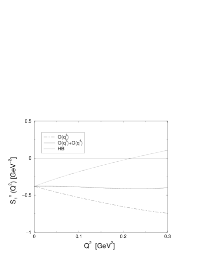
Figure 1: Chiral loop contribution to the structure function $\bar{S}_{1}(0,Q^{2})$ with the elastic contribution subtracted. The solid (dot-dashed) line gives the result of the present calculation to order $q^{4}$ ($q^{3})$ in comparison to the heavy baryon result of [4] (dotted line). Left (right) panel: Proton (neutron).

From these results one deduces the following slopes for the proton and neutron structure function $\bar{S}_{1}(Q^{2})$ (from here on, we do not display the argument $\nu=0$ any longer):

$$\frac{d\bar{S}_{1}^{p}(Q^{2})}{dQ^{2}}\Bigl{|}_{Q^{2}=0} = (-0.4+1.2)~{}{\rm GeV}^{-4}=0.8~{}{\rm GeV}^{-4}~{},$$ (6)

$$\frac{d\bar{S}_{1}^{n}(Q^{2})}{dQ^{2}}\Bigl{|}_{Q^{2}=0} = (-1.7+1.9)~{}{\rm GeV}^{-4}=0.2~{}{\rm GeV}^{-4}~{},$$ (7)

where the first (second) term in the round brackets refers to the third (fourth) order contribution. These results are compatible with expectations from naive dimensional analysis. For comparison, the corresponding HBCHPT results are $d\bar{S}_{1}^{p}/dQ^{2}=2.9\,$GeV^-4 and $d\bar{S}_{1}^{n}/dQ^{2}=2.4\,$GeV^-4, which are quite different. The large slope in the heavy baryon case is due to a variety of effects. First, the large value of the isovector anomalous magnetic moment, $\kappa_{v}=3.71$, appearing in $d\bar{S}_{1}/dQ^{2}\propto[1+3\kappa_{v}+2(1+3\kappa_{s})\tau_{3}]$ leads to a prefactor for the proton of 14 instead of the expected order of one based on naive dimensional analysis. Second, as as been spelled out clearly in [16], in the spin sector the natural expansion parameter seems to be $\pi M_{\pi}/m$ rather than $M_{\pi}/m$ (for the odd powers), which can lead to sizeable corrections. Consequently, the $1/m$ expansion converges slowly, and thus the numbers for these slopes found here should be considered more reliable. Note also that for these slopes the relative size of the fourth order corrections comes out very different for the proton and the neutron, but it should be stressed that the meaningful numbers are the full one–loop (third and fourth order) results. For orientation, we quote the result of the dispersive analysis of [17], which besides pion loop effects also includes resonance contributions, it is $d\bar{S}_{1}^{p}/dQ^{2}=1.8\,$GeV^-4.

In Fig. 2 we show the first moments $\Gamma_{1}^{p}(Q^{2})$ and $\Gamma_{1}^{n}(Q^{2})$ in comparison to the heavy baryon results. For the range of photon virtualities below $Q^{2}=0.2\,(0.3)\,$GeV², the fourth order corrections are not dramatically large for the proton (neutron). Note that while $\Gamma_{1}^{p}(Q^{2})$ crosses zero at $Q^{2}\simeq 0.33\,$GeV², $\Gamma_{1}^{n}(Q^{2})$ stays negative for all values of $Q^{2}$ in the range of virtualities considered here. We stress again that for a direct comparison with the data, some resonance contributions have to be added, this will be done and discussed in the upcoming work [13]. However, one does not expect these resonance contributions to be overly large.

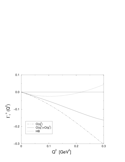
Figure 2: Chiral loop contribution to the first moment $\Gamma_{1}(Q^{2})$. The solid (dot-dashed) line gives the result of the present calculation to order $q^{3}$ ($q^{4})$ in comparison to the heavy baryon result of [4] (dotted line). Left (right) panel: Proton (neutron).

Note that we refrain from comparing these curves with the preliminary data from Jefferson Laboratory because these data are not yet final and can therefore not be shown. This comparison will be done in [13].

In Fig. 3 we show the result for $\Gamma_{1}^{p-n}(Q^{2})$ in comparison to the HBCHPT result [6]. This should be considered the main result of this paper. For $Q^{2}\leq 0.1\,$GeV², the fourth order IR and the heavy baryon result are very similar. For larger momentum transfer, however, $\Gamma_{1}^{p-n}(Q^{2})$ grows faster with increasing momentum compared to the heavy baryon calculation. This is due to the fact that the chiral corrections to the individual $\Gamma_{1}^{p}(Q^{2})$ and $\Gamma_{1}^{n}(Q^{2})$ are quite different (similar) in the IR (HB) approach (for $Q^{2}\geq 0.1\,$GeV²). The corresponding slope is of course given by the GDH sum rule,

$$\frac{d\Gamma_{1}^{p-n}(Q^{2})}{dQ^{2}}\Bigl{|}_{Q^{2}=0}=\frac{\kappa_{n}^{2}-\kappa_{p}^{2}}{8m^{2}}=0.063~{}{\rm GeV}^{-2}~{},$$ (8)

as can also been seen in the figure since all curves merge to one around $Q^{2}\simeq 0$.

Figure 3: First moment difference $\Gamma_{1}^{p}-\Gamma_{1}^{n}$. The solid and the dot-dashed line stand for the chiral expansion at fourth and third order, respectively, using the Lorentz–invariant approach and the dotted line represents the result of the heavy baryon formalism [4, 6].

It is also interesting to consider the slopes corresponding to the combination $\bar{S}_{12}(Q^{2})\equiv\bar{S}_{1}(0,Q^{2})-(Q^{2}/m)$ $\times(d\bar{S}_{2}(\nu,Q^{2})/d\nu)|_{\nu=0}$ for the proton and the neutron case separately, we find

$$\frac{d\bar{S}_{12}^{p}(Q^{2})}{dQ^{2}}\Bigl{|}_{Q^{2}=0} = (3.2+1.8)~{}{\rm GeV}^{-4}=5.0~{}{\rm GeV}^{-4}~{},$$ (9)

$$\frac{d\bar{S}_{12}^{n}(Q^{2})}{dQ^{2}}\Bigl{|}_{Q^{2}=0} = (-0.3-1.8)~{}{\rm GeV}^{-4}=-2.1~{}{\rm GeV}^{-4}~{},$$ (10)

which should be compared with the heavy baryon results [2, 4], $d\bar{S}_{12}^{p}(Q^{2})/dQ^{2}=3.7\,(1-2.6)~{}{\rm GeV}^{-4}=-6.0~{}{\rm GeV}^{-4}$ and $d\bar{S}_{12}^{n}(Q^{2})/dQ^{2}=3.7\,(1-2.1)~{}{\rm GeV}^{-4}=-4.3~{}{\rm GeV}^{-4}$. We remark that the seemingly overwhelming fourth order correction for the neutron is simply a reflection of the accidentally suppressed third order result. The 50% correction found for the proton is not uncommon for the nucleon spin sector. The larger corrections in HBCHPT are simply a reflection of the various effects discussed already before, In the IR approach used here, higher order $1/m$ corrections (in the HBCHPT counting) tend to diminish such large corrections. We point out that such effects also appear in other observables, like e.g. in pion photoproduction off nucleons, but in that case their effect is much less dramatic because they are accompanied by small or normal prefactors (less than or of order one) or do not play a significant role. Such large corrections are only appearing in the spin sector and their origin is essentially understood. Note further that the slope of the integrals $I_{p,n}(0)$ defined in [2] differ from the conventions used here by an overall factor of $\pi/2$. For this combination of the structure functions, one has to include the $\Delta$ (and other resonance) contribution for a direct comparison with the data, see e.g. [2].

5. In this paper, we have considered the one–loop representation of the structure functions of doubly virtual Compton scattering at low photon virtualities, $\bar{S}_{i}(0,Q^{2})$, $i=1,2$ (with the elastic intermediate state contribution subtracted). We have performed the analysis in the framework of infrared regularized relativistic baryon chiral perturbation theory and compared the results with the existing ones obtained in the heavy mass formalism. We have found that there are significant differences for the individual structure functions $S_{1}^{p}(0,Q^{2})$ and $S_{1}^{n}(0,Q^{2})$, i.e. these exhibit a less dramatic (stronger) $Q^{2}$–evolution for the proton (neutron) than in HBCHPT and show reasonable convergence for small photon virtualities. We have also pointed out that the $1/m$ expansion underlying the heavy baryon approach is only slowly converging for these structure functions and thus the resummation of recoil effects inherent to the IR formalism is to be considered important. Clearly, these predictions should only be compared to data when the missing resonance contributions are included. However, in the first moment difference $\Gamma_{1}^{p-n}(Q^{2})$, contributions from spin–3/2 resonances like the delta drop out (and most other resonance contributions, too), so that the predictions shown in Fig.3 should be considered the main result of this paper. As it turns out, the growth of $\Gamma_{1}^{p-n}(Q^{2})$ with increasing $Q^{2}$ is stronger to what was found previously in the heavy mass formulation. It would be interesting to compare this prediction with the data soon becoming available from Jefferson Laboratory. It is important to systematically add resonance contributions to these chiral predictions for the proton and the neutron separately to allow for a direct comparison with the data. Work along these lines is underway [13].

Acknowledgments

We thank Volker Burkert for some useful communications and Norbert Kaiser for comments. One of us (UGM) thanks Susan Gardner and Wolfgang Korsch for their hospitality at the University of Kentucky, where part of this work was done.

Note added

After submission of this manuscript, new experimental information on the integral $I_{n}(Q^{2})$ for $Q^{2}=0.1-0.9\,$GeV² appeared (M. Amarian et al. [The Jefferson Lab E94010 Coll.], arXiv:nucl-ex/0205020). The point at lowest photon virtuality is in good agreement with the prediction given here, but the prediction at $Q^{2}=0.26\,$GeV² is much more negative than the data.

References

- [1] S. B. Gerasimov, Yad. Fiz. 2, 598 (1965) [Sov. J. Nucl. Phys. 2, 430 (1966)]; S. D. Drell and A. C. Hearn, Phys. Rev. Lett. 16, 908 (1966).
- [2] V. Bernard, N. Kaiser and Ulf-G. Meißner, Phys. Rev. D 48, 3062 (1993) [arXiv:hep-ph/9212257].
- [3] X. D. Ji and J. Osborne, J. Phys. G 27, 127 (2001) [arXiv:hep-ph/9905410].
- [4] X. D. Ji, C. W. Kao and J. Osborne, Phys. Lett. B 472, 1 (2000) [arXiv:hep-ph/9910256].
- [5] T. R. Hemmert, B. R. Holstein and J. Kambor, J. Phys. G 24, 1831 (1998) [arXiv:hep-ph/9712496].
- [6] V. D. Burkert, Phys. Rev. D 63, 097904 (2001) [arXiv:nucl-th/0004001].
- [7] J. Edelmann, N. Kaiser, G. Piller and W. Weise, Nucl. Phys. A 641, 119 (1998) [arXiv:nucl-th/9806096].
- [8] T. Becher and H. Leutwyler, Eur. Phys. J. C 9, 643 (1999) [arXiv:hep-ph/9901384].
- [9] P. J. Ellis and H. B. Tang, Phys. Rev. C 57, 3356 (1998) [arXiv:hep-ph/9709354].
- [10] B. Kubis and Ulf-G. Meißner, Nucl. Phys. A 679, 698 (2001) [arXiv:hep-ph/0007056].
- [11] N. Fettes, Ulf-G. Meißner, M. Mojžiš and S. Steininger, Annals Phys. 283, 273 (2001) [arXiv:hep-ph/0001308]; [Erratum-ibid. 288, 249 (2001)].
- [12] V. Bernard, N. Kaiser and Ulf-G. Meißner, Int. J. Mod. Phys. E 4, 193 (1995) [arXiv:hep-ph/9501384].
- [13] V. Bernard, T. R. Hemmert and Ulf-G. Meißner, in preparation.
- [14] V. D. Burkert and B. L. Ioffe, J. Exp. Theor. Phys. 78 (1994) 619 [Zh. Eksp. Teor. Fiz. 105 (1994) 1153].
- [15] V. Burkert and Z. J. Li, Phys. Rev. D 47 (1993) 46.
- [16] G. C. Gellas, T. R. Hemmert and Ulf-G. Meißner, Phys. Rev. Lett. 85 (2000) 14 [arXiv:nucl-th/0002027].
- [17] D. Drechsel, S. S. Kamalov and L. Tiator, Phys. Rev. D 63 (2001) 114010 [arXiv:hep-ph/0008306].
- [18] R. De Vita, talk given at BARYONS 2002, Newport News, Virginia, USA, March 3-8, 2002, see http://www.cebaf.gov/baryons2002/program.html.