DCPT-02/38

IPPP-02/19

Dynamical Generation of Scalar Mesons

M. Boglione

and

M.R. Pennington

Institute for Particle Physics Phenomenology,

University of Durham, Durham DH1 3LE, UK

Starting with just one bare seed for each member of a scalar nonet, we investigate when it is possible to generate more than one hadronic state for each set of quantum numbers. In the framework of a simple model, we find that in the $I=1$ sector it is possible to generate two physical states with the right features to be identified with the $a_{0}(980)$ and the $a_{0}(1450)$. In the $I=1/2$ sector, we can generate a number of physical states with masses higher than $1$ GeV, including one with the right features to be associated with the $K_{0}^{*}(1470)$, but none which can be identified with the light $\kappa$ scalar meson. The $I=0$ sector is the most complicated and elusive: since all outcomes are very strongly model dependent, we cannot draw any robust conclusion. Nevertheless, we find that in that case too, depending on the coupling scheme adopted, the occurrence of numerous states can be achieved. This shows that dynamical generation of physical states is a possible solution to the problem of accounting for more scalar mesons than can fit in a single nonet, as experiments clearly deliver.

          PACS numbers: 12.40.Yx, 13.75.Lb, 14.40.Cs, 14.40.Ev

1 Introduction

In the naive quark model picture with three flavours, quarks and antiquarks are assumed to be bound into states, the quantum numbers of which are determined by the spin $S$ and the relative orbital angular momentum $L$ of the $\overline{q}q$ system. This leads to the multiplet structures that can be elegantly described by the $SU(3)$ group of flavor symmetry. The masses of hadrons are then related to the constituent masses of the quarks and simple relations among them are found. For instance, the non-strange $\rho$ and $\omega$ vector mesons, both made out of up and down quarks, have roughly the same mass, whereas the $\phi$, being a pure $s\overline{s}$ state has a mass approximately 300 MeV heavier. Furthermore, the mass of a meson like the $\rho$, made of two constituent quarks, is about 2/3 of the mass of a proton or a neutron, made of three such quarks. However, the simple and successful picture that the quark model delivers does not apply to the scalar meson sector: apparently scalars are different. First of all there are far more scalar mesons than can be accomodated in one conventional nonet, moreover their masses turn out to be hundreds of MeV lighter than one would simply deduce from the constituent structure of the mesons.

In Ref. [1], Tornqvist presented a model in which the central focus is to consider the loop contributions given by the hadronic intermediate states that each meson can access: it is via these hadronic loops that the bare states become “dressed”  and, in the case of scalar mesons, hadronic loop contributions totally dominate the dynamics of the process. He shows that the mass shift, which is a direct consequence of the presence of strongly coupled hadronic intermediate states, is so dramatic that it completely spoils the one–to–one correspondence between the resonances we observe and the underlying constituent structure. Though we follow Tornqvist’s modelling quite closely, very similar models have been considered by van Beveren et al. [2], Geiger and Isgur [3] and by Oller and Oset [4] among others.

In this paper, following and extending the method of Tornqvist and Roos [5], we will investigate the possibility of generating, in the scalar sector, more than one state with the same quantum numbers, by initially inserting only one “bare seed”. We will show that the outcome depends on the kinematics of the intermediate channels: crucially, on the number and position of each threshold opening and on the strength of their individual couplings. Therefore, every case has to be considered separately and it is not possible to reach one common conclusion for all the members of the scalar meson family.

2 The model of hadronic dressing

We start by considering a simple model in which all bare meson states belong to ideally mixed quark multiplets. We call $n\overline{n}$ the nonstrange light state and suppose that substituting a strange quark for a light one increases the mass of the state by $\Delta m_{s}\simeq 150$ MeV.

The bare propagator for each of these bound states will be of the form

$$P\,=\,\frac{1}{{\cal{M}}_{0}^{2}-s}\;,$$ (1)

with a pole on the real axis, corresponding to a non decaying state; for example for the vector $I=0$ state

$$|\phi\rangle_{0}=|s\overline{s}\rangle.$$

If we now assume that the experimentally observed hadrons are obtained from the bare states ($n\overline{n}$, $s\overline{n}$, $s\overline{s}$, …) by dressing them with hadronic interactions, the propagator becomes

$$P(s)\,=\,\frac{1}{{\cal{M}}^{2}(s)-s-i\,{\cal{M}}(s)\,\Gamma(s)}\;,$$ (2)

where a sum over all hadronic interactions (in the loop) is implicit (see Fig. 1). The pole then moves in the complex $s$-plane.

 

Figure 1: Pictorial representation of the full propagator in Eq. (2).

The corresponding vector state can be decomposed as

$$|\phi\rangle=\sqrt{1-\epsilon^{2}}|s\overline{s}\rangle+\epsilon_{1}|K\overline{K}\rangle+\epsilon_{2}|\rho\pi\rangle+...$$ (3)

where calculation would give $\epsilon^{2}=|\epsilon_{1}|^{2}+|\epsilon_{2}|^{2}+...\ll 1$. The hadronic loop contributions allow the bare states ($s\overline{s}$ in this example) to communicate with all hadronic channels permitted by quantum numbers, and this enables the meson to decay, its lifetime being inversely proportional to the width $\Gamma$. However, in this case the switching on of interactions produces a relatively tiny effect and the physical $\phi$ is still overwhelmingly an $s\overline{s}$ state. For this reason the naive quark model works very well; so from the observed hadron we can easily infer its quark structure. A similar picture works for the tensors.

For scalar mesons the situation is different and the one–to–one correspondence between the observed scalar mesons and their underlying quark content is distorted by dynamical effects. This is because they couple strongly to more than one meson-meson channel, creating overlapping and interfering resonance structures. Furthermore, since the interactions are $S$–waves, the opening of each threshold produces a more dramatic $s$-dependence in the propagator. At each threshold, there is a centrifugal barrier factor of $k^{L}$, where $k$ is the appropriate c.m. $3$-momentum of the decaying products and $L$ their relative orbital angular momentum. This means that the thresholds for higher spin states open more smoothly.

Let us now go into more detail about the model starting, for simplicity, from the case in which only one underlying bare state has to be considered. This is the case, for example, for the $I=1/2$ and $I=1$ sectors, the seeds of which are $s\overline{n}$ and $n\overline{n}$ respectively. We define a vacuum polarization function $\Pi(s)$ which accounts for all the possible two pseudoscalar loop contributions to the propagator $P(s)$ [1]. Referring to the pictorial representation of Eq. (2) in Fig. 1, we can easily write $\Pi$’s imaginary part:

$${\rm Im}\Pi(s)\,=\,-\sum_{i}G_{i}^{2}(s)\,=\,-\sum_{i}g_{i}^{2}\,\frac{k_{i}(s)}{\sqrt{s}}\,(s-s_{A,i})\,F_{i}^{2}(s)\,\theta(s-s_{th,i})$$ (4)

where the index $i$ runs over the pseudoscalar channels and the $k_{i}$’s are the c.m. momenta of the two intermediate pseudoscalars. The $g_{i}$’s are the $SU(3)$ flavour couplings connecting the bare state to the two–pseudoscalar loop: $g_{i}=\gamma\gamma_{i}$, see Refs. [6, 1] for more details. The terms $(s-s_{A,i})$ give the Adler zeros, required for $S$–waves by chiral dynamics. $F_{i}(s)$ are the form factors, which take into account the fact that the interaction is not pointlike but has a spatial extension.

Since the vacuum polarization function, $\Pi(s)$, is an analytic function, its real part can be deduced from the imaginary part by making use of a dispersion relation

$${\rm Re}\,\Pi(s)\,=\,\frac{1}{\pi}P\int_{s_{th,1}}^{\infty}ds^{\prime}\;\frac{{\rm Im}\Pi(s^{\prime})}{s^{\prime}-s}\;.$$ (5)

No subtraction is needed, since the form factors are built in such a way that they decrease fast enough when $|s|\to\infty$.

At this point, we can write the propagator in terms of the vacuum polarization function:

$$P(s)\,=\,\frac{1}{m_{0}^{2}+\Pi(s)-s}$$ (6)

The mass and the width of the decaying hadron are determined, in a process independent way, by the pole of the propagator. Consequently, in order to find the pole position, we have to continue Eqs. (4, 5, 6) into the complex $s$–plane onto the appropriate unphysical sheets.

The contribution of this resonance pole to the $i\to j$ amplitude is then

$$\,\,A_{ij}(s)\,=\,\frac{G_{i}(s)\,G_{j}(s)}{m_{0}^{2}+\Pi(s)-s}\;.$$ (7)

which respects the unitarity requirement, $A-A^{\dagger}=2i\,AA^{\dagger}$. As a consequence, for each elastic channel we can define a resonant phase-shift by

$$A_{ii}(s)\,=\,\frac{1}{2i}\,\left(\eta_{i}\ e^{2i\delta_{i}}\,-\,1\right)\;.$$ (8)

The amplitude $A_{ij}$ in Eq. (7) represents a generalization of the well-known Breit-Wigner formula, at least in the neighbourhood of the pole. This is readily seen by writing the vacuum polarization function in terms of its real and imaginary parts, then

$$A_{ij}(s)\,=\,\frac{G_{i}(s)\,G_{j}(s)}{m_{0}^{2}+{\rm Re}\Pi(s)-s+i{\rm Im}\Pi(s)}\,=\,\frac{m_{R}[\Gamma_{i}(s)\Gamma_{j}(s)]^{1/2}}{m^{2}(s)-s-i\,m_{R}\Gamma_{tot}(s)}\;,$$ (9)

having identified

$$\Gamma_{tot}(s)=-\frac{{\rm Im}\Pi(s)}{m_{R}}=\sum_{i}\,\Gamma_{i}(s)\;,$$ (10)

where

$$\Gamma_{i}(s)=\frac{G_{i}^{2}(s)}{m_{R}}\;,$$ (11)

and

$$m^{2}(s)=m_{0}^{2}+{\rm Re}\Pi(s)\;.$$ (12)

Here $m^{2}(s)$ is the running squared mass, given by the sum of the bare mass squared and the real part of the vacuum polarization function ${\rm Re}\Pi(s)$, which is responsible for the mass shift. The imaginary part of the vacuum polarization function ${\rm Im}\Pi(s)$ is directly proportional to the width of the state. The mass shift function ${\rm Re}\Pi(s)$ is generally negative and is approximately constant only in the energy regions far from any threshold. For $S$–waves the $s$–dependence becomes crucially important nearby thresholds, since ${\rm Re}\Pi(s)$ has square root cusps at the opening of each of them.

Though the only correct way to calculate the mass of a particle is to find the position of the propagator pole in the complex $s$–plane, it is useful to define another quantity, again obtainable from the propagator, which we will call the Breit–Wigner mass $m_{BW}$. It corresponds to the intersection of the running mass $m^{2}(s)$ with the curve $s$, i.e. the particular value of $s$ where the function $(m_{0}^{2}+{\rm Re}\Pi(s)-s)$ vanishes, with $s$ wholly real:

$$m^{2}_{BW}=m_{0}^{2}+{\rm Re}\Pi(m^{2}_{BW})\;.$$ (13)

This gives a rough estimate of what the physical mass is. As a matter of fact, moving into the complex plane the real coordinate of the pole position can change considerably if thresholds to strongly coupled channels are located nearby, and when the dynamics are particularly complicated. As $m_{BW}$ of Eq. (13) is defined as the energy at which the function $m^{2}(s)$ is equal to $s$, this is a point that we refer to as a crossing for reasons that will become clear in Fig. 2. Clearly at $\sqrt{s}=m_{BW}$, the amplitudes $A_{ij}$ of Eq. (9) become purely imaginary. It is this simple fact and its physical consequences that are the theme of this paper.

3 $I=1$ sector and the role of the Wigner condition

We now turn our attention to the issue of accomodating all the scalar meson states (which experiments deliver) in either one or more quark model multiplets. In Ref. [1] Tornqvist finds a scalar nonet composed of the $K_{0}^{*}(1430)$, the $a_{0}(980)$, the $f_{0}(980)$ and the $f_{0}(1370)$. Furthermore, in Ref. [5], one extra low energy pole is found, which the authors identify with the much discussed broad $\sigma$ meson, called $f_{0}(400-1200)$ in the Particle Data Tables [7]. Nevertheless, this study leaves out the $a_{0}(1430)$, for instance, for which Crystal Barrel [8] finds clear evidence.

Consequently, we begin by examining the $I=1$ sector, since this is relatively simpler than the others. We ask: can we “generate” one or more extra physical states in the same sector, in the framework of our simple model, by starting from only one $\overline{n}n$ bare seed ?

 

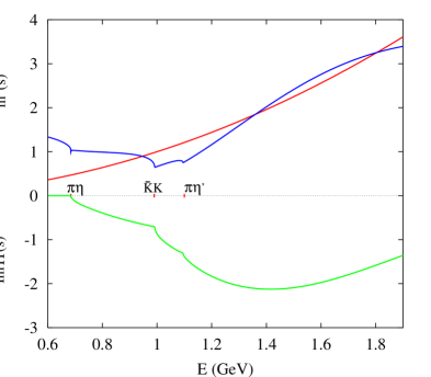
Figure 2: The curves $m^{2}(s)$, $s$ and $\rm Im\Pi(s)$ as functions of the energy $E\ =\ \sqrt{s}$, for the sector $I=1$. Each intersection between $m^{2}(s)$ and $s$ is referred to as a crossing. The first of these is situated at approximately $915$ MeV, between the $\pi\eta$ and the $K\overline{K}$ threshold. The second crossing, well above the $\pi\eta^{\prime}$ threshold, is at $E=1430$ MeV. The third intersection, at $1.82$ GeV, is a non-physical state according to the Wigner condition.

By increasing the overall coupling $\gamma$ and the bare mass of the $\overline{n}n$ seed ($\gamma=1.53$, $m_{0}=1.620$ GeV, as opposed to $\gamma=1.13$, $m_{0}=1.420$ GeV used in Ref. [1]), we find it is possible to obtain a scenario in which more than one intersection between the mass function $m^{2}(s)$ and the $s$ curve appear in the mass plot, as shown in Fig. 2 (upper half). The first crossing, situated at approximately $915$ MeV, between the $\pi\eta$ and the $K\overline{K}$ threshold, corresponds to a state which can be identified with the $a_{0}(980)$. We treat the charged and neutral kaons as degenerate in mass and so neglect the possibility of isospin mixing between $I=1$ and $I=0$ states [9]. The second crossing, occurring well above the $\pi\eta^{\prime}$ threshold, at $m_{BW}=1430$ MeV, is again a physical state and has the right features to represent the Crystal Barrel relatively broad $a_{0}(1450)$; the third intersection occurs at $E=1.82$ GeV. In the lower half of Fig. 2 we plot the curve $\rm Im\Pi(s)$, which shows how the second state which we identify with the $a_{0}(1450)$ is much broader than the $a_{0}(980)$.

To know which state is physical we refer to the Wigner condition [10]. This condition follows from the principle of causality, i.e. the requirement that the scattered wave does not leave the scatterer before the incident wave has reached it. In the present context, Wigner’s theorem limits the rate of fall of the phase-shift, $\delta_{ij}$. A physical resonance cannot occur if the phase shift falls through $90^{o}$. In fact, such a resonance would have a negative width and correspond to a pole on the upper half plane in the physical sheet. It would therefore represent a non-causal, exponentially increasing state. Since it is not possible to have a state with a lifetime greater than the period of scattering, Wigner’s condition requires

$$\frac{d\delta}{dk}\geq-\frac{1}{m_{\pi}}\frac{\sqrt{s}}{2k}.$$ (14)

where the phase-shift $\delta$ refers to the same channel as the c.m. 3-momentum $k$ and is defined by Eq. (8). The Wigner condition is particularly useful in the inelastic region, where resonances do not necessarily correspond to $\delta=90^{o}$, but more generally occur when $\delta=n\pi/2$ and the real part of the scattering amplitude is zero.

$$\begin{array}[]{ll}\mbox{~{}\psfig{angle=-90,width=227.62204pt}}&\mbox{~{}\psfig{angle=-90,width=227.62204pt}}\end{array}$$

Figure 3: The phase $\delta_{\pi\eta}$ reaches $90^{o}$ at $E=915$ MeV, corresponding to the first physical state identified with the $a_{0}(980)$ (the point is labelled by a star on the left hand plot). The phase $\delta_{\pi\eta^{\prime}}$ reaches zero twice (the two points are labelled on the right hand plot), the first time raising from negative to positive values and giving the second physical $a_{0}$ state, the second time quickly dropping from positive to negative values, and delivering the unphysical third state, as confirmed by the Wigner condition.

 

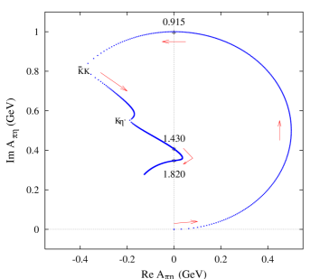
Figure 4: Argand plot of the amplitude $A_{\pi\eta}$: in the elastic region, Im$A_{\pi\eta}$ raises quickly anti-clockwise and Re$A_{\pi\eta}$ reaches zero at $E=915$ MeV, the lighter physical $a_{0}$. The second and third states occur above $\pi\eta^{\prime}$ threshold, as indicated by the two stars on the plot. Notice that the heavy unphysical state is situated immediately after an abrupt change of direction in the curve Im$A_{\pi\eta}$.

Fig. 3 shows the phases, $\delta_{\pi\eta}$ and $\delta_{\pi\eta^{\prime}}$, which tell us about the characteristics of the states we find: $\delta_{\pi\eta}$ goes through $90^{o}$ at $E=915$ MeV, in correspondence with the first physical resonance, the lighter $a_{0}$. Instead, $\delta_{\pi\eta^{\prime}}$ reaches zero twice: the first time rising from negative to positive values and giving the second physical $a_{0}$ state, the $a_{0}(1450)$; the second time quickly dropping from positive to negative values: the third crossing at 1820 MeV is unphysical as given by Eq.(14).

Finally, Fig. 4 shows the Argand plot of the amplitude $A_{\pi\eta}$: in the elastic region, Im$A_{\pi\eta}$ rises quickly anti-clockwise and Re$A_{\pi\eta}$ reaches zero at $E=915$ MeV, the lighter physical $a_{0}$. The second and third states occur above $\pi\eta^{\prime}$ threshold, as indicated by the two stars on the plot. Notice that the heavy unphysical state is situated immediately after an abrupt change of direction in the curve Im$A_{\pi\eta}$.

Our conclusions about yet heavier states are not reliable in the present model, since higher thresholds are not included which may well affect the picture at higher energies dramatically. Nevertheless just including the lightest two pseudoscalar channels we can definitely say that a scenario in which not only one but a series of scalar physical states with I=1 can easily be achieved, by fine tuning key free parameters of the model.

Generating more than one physical state with the same quantum number starting from one seed brings us closer to the picture emerging from experiment. Will this be the case for the other sectors as well ? And to what extent is the adjustment of the overall coupling and mass parameters permitted within this model? That is what we discuss in the following Sections.

4 The $I=1/2$ sector

In an analogous manner to the $I=1$ case, we now want to examine the possibility of dynamically generating more physical states with the same quantum numbers from only one bare seed, $n\overline{s}$ in this particular case. Here the main issue is to investigate whether it is possible to generate the light $I=1/2$ state called $\kappa$, advocated for example in Refs. [4, 11, 2].
The situation for the $I=1/2$ sector is rather different from the $I=1$ case. Here there are only two relevant thresholds and their positions and coupling strengths are such that the shape of the mass function curve, $m^{2}(s)$, is very rigid and varying the parameters changes this little. Nevertheless, by using the same changes we used for the $I=1$ sector ($\gamma=1.53$, $m_{0}=1.620$ GeV, with $s_{A,\pi K}=-1.0$ GeV²) we obtain the plot shown in Fig 5.

The first interesting observation is that the first point of intersection between the mass function $m^{2}(s)$ and the curve $s$, is always bound to be below the $K\pi$ threshold and it corresponds to a pole on the real axis, i.e. to a state with zero width: in fact, the cusp signals the precise location of the threshold itself, so that varying the coupling strength only slightly alters the position of the crossing point, but never allows it to move above the threshold.

 

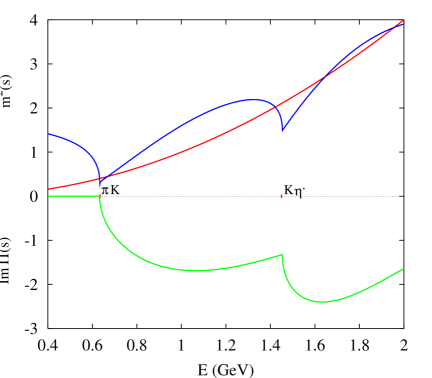
Figure 5: The curves $m^{2}(s)$, $s\ =\ E^{2}$ and $\rm Im\Pi(s)$ as functions of the energy $E$. The first crossing point is located below the $K\pi$ threshold and corresponds to a pole on the real axis (i.e. a non-decaying state). The second crossing is again an unphysical state because it does not satisfy the Wigner condition, as clearly shown by the phase shift and the Argand plot in Figs. 7 and 7. On the contrary, the third intersection point corresponds to an unphysical state. Finally the last two crossings correspond to a non-physical and a heavier and broader physical state respectively.

The second intersection point is not a physical state since it violates the Wigner condition, as is clearly shown by the phase shift and the Argand plot in Figs. 7 and 7. Notice once again that the conclusion that this state is not physical does not depend on the strength of the coupling to the $K\pi$ channel: varying this only produces a tiny shift in the position of the crossing point, and does not alter the characteristics of the state. Thus within this model having just one $n\overline{s}$ bare seed, it turns out to be impossible to generate a physical $\kappa$-like state. In contrast, the third intersection point corresponds to a physical state which can easily be interpreted as the $K_{0}^{*}(1430)$, already found in Tornqvist results of Ref. [1]. It is interesting to notice that the same kind of picture would emerge when using the parameterization proposed in Ref. [5]: the first crossing point is again below threshold and the second one corresponds to a state which, violating the Wigner condition, is unphysical. Indeed, only the third intersection point is a physical one.

Moving to higher energies, we find two further crossing points between the $s=E^{2}$ curve and the mass function $m(s)^{2}$: according to the Wigner condition, only the last one, situated at $E=1.96$ GeV, corresponds to a physical state. As we mentioned in the previous Section, results concerning states with heavy masses are not completely reliable since the present model does not include higher meson-meson thresholds. Nevertheless, it is quite interesting to notice that the last physical state predicted by our calculation could be identified with the $K_{0}^{*}(1950)$ reported by the PDG group (see table on p. 51 of Ref. [7]).

Compared with other results available in the literature, as far as the $I=1/2$ and $I=1$ sectors are concerned, ours are similar to those presented in the work of Minkowski and Ochs [12], where they claim the existence of two complete nonets in the light scalar meson spectrum, the first one characterised by the $K_{0}^{*}(1430)$ and the $a_{0}(980)$, and the second one by the $K_{0}^{*}(1950)$ and the $a_{0}(1450)$. To the isoscalar sector they assign the $f_{0}(980)$, $f_{0}(1500)$ and the $f_{0}(1720)$, $f_{0}(2020)$ respectively, with singlet-octet mixing angle (much as in the pseudoscalar nonet), having dismissed the $\sigma$ and the $f_{0}(1370)$.
In contrast, van Beveren et al. [2] find two lower mass nonets, given by

$$\kappa,\;a_{0}(980),\;f_{0}(980),\;\sigma$$

$$K_{0}^{*}(1430),\;a_{0}(1450),\;f_{0}(1370),\;f_{0}(1500)\;,$$

whereas Shakin and collaborators [13] predict the existence of up to three scalar nonets, characterized by

$$a_{0}(980),\;K_{0}^{*}(1430)$$

$$a_{0}(1450),\;K_{0}^{*}(1730)$$

$$a_{0}(1857),\;K_{0}^{*}(1950)$$

and keep the $\sigma$ and $\kappa$ mesons out, using their particular definition of “dynamically generated states” with no right to be classified into a nonet structure. Moreover the $a_{0}(1857)$ and the $K_{0}^{*}(1730)$ are resonances which appear in their calculation but are not confirmed by experiment yet.

To complete our picture we now move to the $I=0$ sector.

$$\begin{array}[]{ll}\mbox{~{}\includegraphics[width=170.71652pt,angle={-90}]{kph1.ps}}&\mbox{~{}\includegraphics[width=170.71652pt,angle={-90}]{kph2.ps}}\end{array}$$

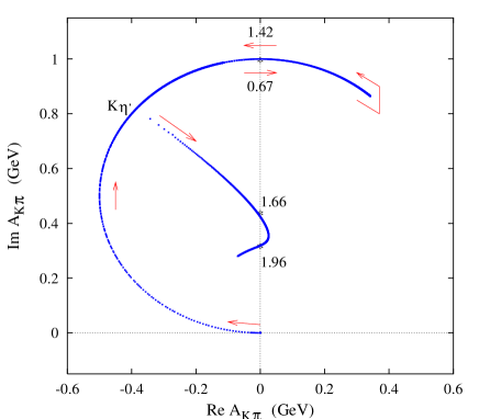
Figure 6: The phase $\delta_{K\pi}$ drops extremely quickly through $90^{o}$ at $E=670$ MeV, in correspondence with the unphysical state generated by the second crossing point in Fig. 5. It then rises through $90^{o}$ at $E=1420$ MeV, signalling the presence of a physical state, (the two points are labelled on the left hand plot). The phase $\delta_{K\eta^{\prime}}$ goes through $90^{o}$ twice (the two points are each labelled by a star on the right hand plot), the first time decreasing quickly from $180^{o}$ at $K\eta^{\prime}$ threshold, giving the third unphysical state, the second time while increasing again to larger values, and delivering the last physical state, as confirmed by the Wigner condition.

Figure 7: Argand plot of the amplitude $A_{K\pi}$: in the elastic region, Im$A_{K\pi}$ raises quickly clockwise and Re$A_{K\pi}$ reaches zero at $E=670$ MeV, corresponding to the first unphysical state. It then goes back anti-clockwise and Re$A_{K\pi}$ reaches zero again at $E=1420$ MeV, signalling the presence of the first physical state, the $K_{0}^{*}(1430)$ (indicated on the plot) by a star. The following unphysical and physical states, with BW masses of $1.66$ and $1.96$ GeV respectively, are situated in the inelastic region, well over the $K\eta^{\prime}$ threshold, and are also indicated on the plot by little stars.

5 The $I=0$ sector

This is the most complex and delicate sector, and drawing any kind of conclusion is particularly difficult: let’s see why. As discussed in the previous Sections, in the $I=1$ and $I=1/2$ sectors physical states originate from one “bare seed” only, either $n\overline{n}$ or $n\overline{s}$, and are then “dressed” by coupling to meson-meson channels. In contrast, in the $I=0$ case we already have two possible “bare seeds” to start with, $n\overline{n}$ and $s\overline{s}$, which not only get dressed but in fact do mix through hadronic loops. And mixing entangles the situation to such an extent that the one–to–one correspondence between the phase shift behaviour and the occurrence of physical states is lost: then the Wigner condition cannot be used to sort the physical states from the unphysical ones. Moreover, the couplings of the isoscalar bare seeds to the relative meson-meson channels, $\pi\pi$, $K\overline{K}$, $\eta\eta$ etc … are not calculated in a standard and unique way: there are several calculations in the literature, each of which is based on different (but in our opinion equally good or bad) assumptions (see for example Refs. [1] and [2]). So one has to make a choice of coupling scheme as well, and unfortunately the outcome strongly depends on this choice.

If we simply use for the parameters $\gamma$ and $m_{0}$ the same values as in Sections 3 and 4 and the coupling scheme as given by Tornqvist in Ref. [1] (with the $\eta\eta^{\prime}$ threshold coupling enhanced by a factor $\beta=1.6$) or by van Beveren et al. [2], we find scenarios in which multiple crossings do occur and many isoscalar states are generated. Unfortunately, we cannot tell them apart, because the phase shift behaviour does not help, especially in the region around and above $1$ GeV, where the mixing is maximal and the overlapping among resonances is crucial. And we cannot say which of them are physical states either, because the Wigner condition cannot be applied. Moreover, as we anticipated, the position and features of the crossing points are very strongly model dependent, and very different scenarios can be created by varying the coupling scheme, so that no robust model independent conclusion can be reached in this sector. For instance, if we apply purely $SU(3)$ pseudoscalar-pseudoscalar couplings, as presented in Refs. [1, 6] without enhancing the $\eta\eta^{\prime}$ threshold, only two resonant states are found.

Nevertheless, it is a fact that a number of states larger than two can be created starting from just two bare seeds. For certain parameter configurations and with certain coupling schemes, the $I=0$ experimental candidates can be accounted for. This shows that the dynamical generation of physical states is a possible solution to the problem of accounting for more scalar mesons than can fit in one nonet. Notice, though, that this is a “democratic” model, in which we cannot distinguish which are the intrinsic (or pre-existing) states as opposed to the dynamically generated ones (a discussion about this issue was raised by van Beveren et al. in a comment [15] on a paper by Shakin and Wang [16]).

6 Scattering amplitudes

To what extent are we free to change the parameters of the model to allow the double crossing to occur that generates the $a_{0}(1430)$ as well as the $a_{0}(980)$? This question is addressed by considering the relationship of the propagators in Eqs. (1,2,6,7) to the corresponding physical scattering amplitudes. As noted in Section 2, knowing the propagator of $s-$channel resonances determines a key part of the scattering amplitudes, Eqs. (7,9). For Tornqvist and Roos, this amplitude $A_{ij}$ is all there is to the hadronic scattering amplitude. However, $s-$channel dynamics is not all that controls the scattering. So while the amplitude $A$ defined in Eq. (7) respects unitarity, it is not the most general amplitude that achieves this, having its numerator and denominator related by the same couplings $G_{i}$ (see Eq. (4)). Knowing the structure of the propagator $P(s)$, Eq. (6), we can write in complete generality the full scattering amplitude as

$$T(s)=\frac{N(s)}{m^{2}(s)-s+\Pi(s)}\;,$$ (15)

where we drop the channel labels $ij$. The numerator $N(s)$ is an unknown complex function of the variable $s$, which can be re–expressed in terms of its modulus and phase as

$$N(s)=|N(s)|\,e^{i\alpha(s)}\;.$$ (16)

Imposing both elastic and inelastic unitarity one finds that

$$|N(s)|=[m^{2}(s)-s+{\rm Re}\Pi(s)]\sin\alpha(s)-{\rm Im}\Pi(s)e^{i\,\alpha(s)}\;,$$ (17)

which allows the most general hadronic amplitude to be written as

$$T(s)\,=\,A(s)\,e^{\,2i\,\alpha(s)}+\sin\alpha(s)\;e^{\,i\,\alpha(s)}$$ (18)

where $\alpha(s)$ is an unknown function of $s$ real along the right hand cut, and the second term in Eq. (18) can be regarded as a background contribution. It is important to note that if the phase-shift of the amplitude $A$ is $\omega$, then the phase-shift of the full amplitude $T$ is $\delta=\omega+\alpha$.
The model of Tornqvist and Roos is to set $\alpha=0$ everywhere.

In Ref. [17] we have improved on Tornqvist’s study by performing new fits to experimental data, based on the general amplitude $T(s)$ rather than the pole dominated amplitude $A(s)$. From this we conclude that very good solutions can be obtained by using relatively small values for the parameter $\alpha$ (we chose a constant value of $15^{o}$ as an example) and varying the $m_{0}$ and $\gamma$ parameters by a few hundred MeV. For instance, to fit $\pi K$ scattering data in terms of the pure pole amplitude $A$, Tornqvist requires the position of the Adler zero to be at $s_{A,\pi K}=-0.42$ GeV² far from its position in chiral perturbation theory (current algebra predicts $(m_{K}-m_{\pi})^{2}\leq s_{A,{\pi K}}\leq(m_{K}+m_{\pi})^{2}$ with an average value of $0.24$ GeV²). In contrast, by a simple choice of $\alpha$ of about $15^{0}$ we can fit these same data with the full hadronic amplitude $T$ which has the Adler zero at the position required by chiral dynamics.

This puts our attempts to generate extra states with the same quantum numbers by varying the free parameters of the model on more solid ground. We know that small changes in the value of $m_{0}$ and $\gamma$ can give equally good fits using the full hadronic amplitudes, $T$. This gives us confidence in our general conclusions. The fact that there is more to a scattering process than $s-$channel dynamics means that fitting data along the real axis cannot accurately determine the true pole position of a broad state without an analytic continuation, or a very specific model. This casts doubt on the determination of the position of the $\sigma-$pole by Tornqvist and Roos. Their fit to $\pi\pi$ data in terms of the amplitude $A$ gives quite different parameters than using the full amplitude $T$ of Eq. (18). That there is more to dynamics than $s$-channel resonances has been noted by Isgur and Speth in this same context [18].

7 Conclusions

The present work focusses on the study of the $I=1$ and $I=1/2$ sector of the light scalar meson spectroscopy. Previous papers from Tornqvist and Roos [1, 5] seemed to suggest that using a simple model based on the hadronic “dressing” of bare seeds, one could generate more than one, possibly a whole family of mesons, with the same quantum numbers, starting with one bare seed only. This is certainly a very interesting possibility, since we know that experiment has detected many more light scalar mesons that can be accomodated in one nonet. We started by investigating the $I=1$ sector, where two strong candidates have been found: the long known $a_{0}(980)$ and the heavier $a_{0}(1450)$, detected by the Crystal Barrel collaboration [19]. By slightly increasing two crucial parameters of the model, the overall coupling $\gamma$ and the bare mass $m_{0}$, we have shown that it is possible to find a picture in which both states can easily be generated starting from one bare $n\overline{n}$ seed only. Due to the structure of the vacuum polarization function, the heavier of the two states is automatically broader than the lighter one. Drawing conclusions on further, heavier states would require detailed treatment of heavier thresholds, which are not included here.

Encouraged by these results we then moved to the $I=1/2$ sector, to try and see whether we could also give a legitimate place to the controversial $\kappa$ meson. Due to the nature of the $n\overline{s}$ couplings to pseudoscalar-pseudoscalar channels, it turns out to be impossible to generate such a light $I=1/2$ scalar meson in our framework. Further heavier states can be generated, one of which has the right features to be identified with the $K_{0}^{*}(1430)$, whereas the others might only be an artifact of the poor treatment of heavy thresholds in the model. Again, only a more rigorous description of such heavier thresholds could enable us to rule out their existence or not.

To complete the study, we considered the $I=0$ sector: even though the heavily structured dynamics of the isoscalars make any clear–cut result far from robust, at least in the framework of our simple model, we can conclude that the multiple crossing mechanism is certainly active in this sector as well, and that dynamical generation of many states with the same quantum numbers but different masses can be a plausible explanation of the experimental occurence of many more $0^{++}$ states that can fit in one quark–model nonet.
We conclude that the detailed pole parameters of Ref. [5] are strongly model dependent, as previously suggested by the comments of Refs. [18].

As opposed to the work in Ref.[16], we cannot tell which are intrinsic states and which are dynamically generated, nor can we state that we have definitely found enough strong candidates to complete two full nonets as in Refs. [12, 2]: we can find no way to produce the light $\kappa$ meson and no precise assignment can be made for the isoscalar sector. As far as the isovector and isodoublet states are concerned, our picture is similar to that of Ref. [12], with the occurrence of two $a_{0}$ and two $K_{0}^{*}$ physical states and the possibility to produce a number of $f_{0}$’s, depending on the coupling scheme.

References

- [1] N.A. Tornqvist, Z. Phys. C 68, 647 (1995).
- [2] E. van Beveren and G. Rupp, Eur. Phys. J. C10, 468 (1999).
- [3] P. Geiger, N. Isgur, Phys. Rev D 47, 5050 (1993).
- [4] J.A. Oller, E. Oset, Phys. Rev. D 59, 074001, (1999).
- [5] N.A. Tornqvist and M. Roos, Phys. Rev. Lett. 76, 1575 (1996).
- [6] N.A. Tornqvist, Acta Phys. Pol. B16, 503 (1985).
- [7] D.E. Groom et al., Review of Particle Physics, Eur. Phys. J. C 15 (2000).
- [8] C. Amsler et al., Phys. Lett. B 333, 277 (1994); 342, 433 (1995); 353, 571 (1995).
- [9] N.N. Achasov, S.A. Devyanin and G.N. Shestakov, Phys. Lett. B 88, 367 (1979).
- [10] E.P. Wigner, Phys. Rev. 98, 145 (1955). See also H. Burkhardt, “Dispersion Relation Dynamics”, North Holland, 1969, p. 199.
- [11] D. Black, A. H. Fariborz, F. Sannino, J. Schecther, Phys. Rev. D 59, 074026 (1999).
- [12] W. Ochs, contribution to the proceedings of the IXth International Conference on Hadron Spectroscopy (HADRON 2001), Protvino, Russia, August 2001, hep-ph/0111309; P. Minkowski and W. Ochs, Eur. Phys. J. C 9, 283 (1999).
- [13] L.S. Celenza, Shun-fu Gao, Bo Huang, Huangsheng Wang, C.M. Shakin, Phys. Rev. C 61, 035201 (2000); C. M. Shakin, Huangsheng Wang, Phys. Rev. D 62, 114014 (2000); Phys. Rev. C 63, 025209 (2001).
- [14] E. van Beveren, T. A. Rijken, K. Metzger, C. Dullemond, G. Rupp and J. E. Ribeiro, Zeit. Phys. C 30 615 (1986).
- [15] E. van Beveren and G. Rupp, Phys. Rev. D 65, 078501, (2002).
- [16] C.M. Shakin and Huangsheng Wang, Phys. Rev. D 63, 014019 (2000).
- [17] M. Boglione, “A Study of Light Scalar Meson Spectroscopy”, PhD Thesis, University of Turin (Italy) and University of Durham (U.K.).
- [18] N. Isgur, J. Speth, Phys. Rev. Lett. 77, 2332 (1996).
- [19] C. Amsler et al., Phys. Lett. B 342, 433 (1995); Phys. Lett. B 353, 571 (1995); Phys. Lett. B 355, 425 (1995).