Hybrid adiabatic potentials in the QCD string model

Abstract

The short- and intermediate-distance behaviour of the hybrid adiabatic potentials is calculated in the framework of the QCD string model. The calculations are performed with the inclusion of Coulomb force. Spin-dependent force and the so-called string correction term are treated as perturbation at the leading potential-type regime. Reasonably good agreement with lattice measurements takes place for adiabatic curves excited with magnetic components of field strength correlators.

1 Introduction

Gluonic degrees of freedom in the nonperturbative region should manifest themselves as QCD bound states containing constituent glue, so one expects that purely gluonic hadrons (glueballs) should exist as well as hybrids where the glue is excited in the presence of $q\bar{q}$ pair. General agreement is that the lightest hybrids occur in the mass range between 1.3 and 1.9 GeV, so the absolute mass scale remains somewhat imprecise in the absence of exact analytic methods of nonperturbative QCD. Existing experimental data seem to point towards gluonic excitations being present, and prima facie candidates are identified [1], but the conclusive evidences have never been presented. There is no hope that in the nearest future data analyses could unambigiously pin-point the signatures for gluonic mesons and settle the issue of constituent glue. The state-of-art is that the predictions of different models on hadronic spectra and decays are involved in order to distinguish between gluonic mesons and conventional ones.

In such situation the lattice gauge calculations remain the only source of knowledge. Lattice calculations are now accurate enough to serve as a guide, so that the results of different QCD-motivated approaches can be compared and contrasted with lattice data. Of particular interest are the measurements of gluelump [2] and hybrid adiabatic potentials [3]. These simulations measure the spectrum of the glue in the presence of static source in the adjoint colour representation (gluelump) and in the presence of static quark and antiquark separated by some distance $R$. These systems are the simplest ones and play the role of hydrogen atom of soft glue studies, as, first, the gluonic effects are not obscured by light dynamical quarks, and, second, the problem of centre-of-mass motion separation is not relevant here.

The large distance limit of hybrid adiabatic potentials is important, as one expects the formation of confining string at large $R$. The short range limit is relevant to the heavy hybrid mass estimations. One expects that in the case of very heavy quarks the hybrid resides in the bottom of the potential well given by the adiabatic curve, which, in accordance with lattice results [3], is somewhere around 0.25 fm for lowest curves.

In the present paper we study hybrid adiabatic potentials in the so-called QCD string model [4]. This model deals with quarks and point-like gluons propagating in the confining QCD vacuum, and is derived from the Vacuum Background Correlators method. In the latter, the confining vacuum is parametrised by the set of gauge-invariant field strength correlators [5] responsible, among other phenomena, for the area law asymptotics. The basic assumption of the QCD string model is the minimal area law for the Wilson loop, so that the only nonperturbative input is the string tension $\sigma$.

The QCD string model describes the spectra of $q\bar{q}$ mesons with remarkable agreement [6],[7]. It is also quite successfull in describing glueballs [8], hybrids [9] and gluelump [10], as well as meson-hybrid-glueball mixing [11].

First studies of hybrid adiabatic potentials in the QCD string model were performed in [12], with special attention paid to the large-distance limit. It was shown that at large interquark distances two kinds of QCD string vibrations take place, the potential-type longitudinal and string-type transverse ones. Here we consider the short-distance behaviour of the excitation curves.

The paper is organised as follows. In Section 2 we briefly discuss the essentials of the QCD string approach for gluons. The effective Hamiltonian for a gluon bound by the static quark-antiquark pair is derived in Section 3. It is argued in Section 4 that at short and intermediate interquark distances the potential-type regime of string vibrations is adequate, and the lowest excitation curves are calculated. The spin-dependent forces and the so-called string corrections are considered in Section 5. Results and discussion are given in Section 6 together with conclusions and outlook. Appendices contain the details of our variational calculations.

2 Gluons in the confining background

The QCD string model for gluons is derived in the framework of perturbation theory in the nonperturbative confining background [13]. The main idea is to split the gauge field as

$$A_{\mu}=B_{\mu}+a_{\mu},$$ (1)

which allows to distinguish clearly between confining field configurations $B_{\mu}$ and confined valence gluons $a_{\mu}$. The valence gluons are treated as perturbation at the confining background.

We start with the Green function for the gluon propagating in the given external field $B_{\mu}$ [13]:

$$G_{\mu\nu}(x,y)=(D^{2}(B)\delta_{\mu\nu}+2igF_{\mu\nu}(B))^{-1},$$ (2)

where both covariant derivative $D_{\lambda}^{ca}$ and field strength $F_{\mu\nu}^{a}$ depend only on the field $B_{\mu}$:

$$D_{\lambda}^{ca}(B)=\delta^{ca}\partial_{\lambda}+gf^{cba}B^{b}_{\lambda},$$ (3)

$$F_{\mu\nu}^{a}(B)=\partial_{\mu}B^{a}_{\nu}-\partial_{\nu}B^{a}_{\mu}+gf^{abc}B^{b}_{\mu}B^{c}_{\nu}.$$ (4)

The term, proportional to $F_{\mu\nu}(B)$ in (2) is responsible for the gluon spin interaction. We neglect it for a moment, it will be considered in Section 5.

Now we use Feynman-Schwinger representation for the quark-antiquark-gluon Green function [9], which, for static quark and antiquark, is reduced to the form

$$G(x_{g},y_{g})=\int^{\infty}_{0}ds\int Dz_{g}\exp(-K_{g})\langle{\cal W}\rangle_{B},$$ (5)

where angular brackets mean averaging over background field. The quantity $K_{g}$ is the kinetic energy of gluon (to be specified below), and all the dependence on the vacuum background field is contained in the generalized Wilson loop $\cal W$, depicted in Fig.1, where the contours $\Gamma_{Q}$ and $\Gamma_{\bar{Q}}$ run over the classical trajectories of static quark and antiquark, and the contour $\Gamma_{g}$ runs over the gluon trajectory $z_{g}$ in (5).

Figure 1: Hybrid Wilson loop

The expression (5) is the starting point of the QCD string model, as, under the minimal area law assumption, the Wilson loop configuration takes the form

$$\langle{\cal W}\rangle_{B}=\frac{N_{c}^{2}-1}{2}\exp(-\sigma(S_{1}+S_{2})),$$ (6)

where $S_{1}$ and $S_{2}$ are the minimal areas inside the contours formed by quark and gluon and antiquark and gluon trajectories correspondingly.

3 Einbein field form of the gluonic Hamiltonian

To proceed further we are to fix the gauge in the reparametrization transformations group. For the case of static quark and antiquark sources the most natural way to do this is to identify the proper time $\tau$ of the Feynman-Schwinger representation with the laboratory time. Then the classical quark and antiquark trajectories are given by

$$z_{Q\mu}=(\tau,\frac{\mbox{\boldmath${\rm R}$}}{2})~{}~{},~{}~{}z_{\bar{Q}\mu}=(\tau,-\frac{\mbox{\boldmath${\rm R}$}}{2})~{}~{},$$ (7)

and the action of the system can be immediately obtained from the representation (5):

$$A=\int^{T}_{0}d\tau\left\{-\frac{\mu}{2}+\frac{\mu\dot{r}^{2}}{2}-\sigma\int^{1}_{0}d\beta_{1}\sqrt{(\dot{w}_{1}w_{1}^{\prime})^{2}-\dot{w}_{1}^{2}w^{{}^{\prime}2}_{1}}-\right.$$

$$\left.-\sigma\int^{1}_{0}d\beta_{2}\sqrt{(\dot{w}_{2}w_{2}^{\prime})^{2}-\dot{w}_{2}^{2}w^{{}^{\prime}2}_{2}}\right\}.$$ (8)

Here ${\rm r}$ is the three-dimensional gluonic coordinate, and the minimal surfaces $S_{1}$ and $S_{2}$ are parametrized by the coordinates $w_{i\mu}(\tau,\beta_{i}),~{}i=1,2,~{}\dot{w}_{i\mu}=\frac{\partial w_{i\mu}}{\partial\tau},~{}w^{\prime}_{i\mu}=\frac{\partial w_{i\mu}}{\partial\beta_{i}}.$ Choosing the straight-line ansatz for the minimal surfaces one has in the laboratory time gauge

$$w_{i0}=\tau,~{}~{}~{}\mbox{\boldmath${\rm w}$}_{1,2}=\pm(1-\beta)\frac{\mbox{\boldmath${\rm R}$}}{2}+\beta\mbox{\boldmath${\rm r}$}.$$ (9)

The kinetic energy in (8) is given in the so-called einbein field form [14]. The einbein field $\mu=\mu(\tau)$ is the auxiliary field introduced to deal with relativistic kinematics. Note that in the case of gluon one is forced to introduce it from the very beginning, as it provides the meaningful dynamics for the massless particle.

In order to pass to the Hamiltonian formulation it is convenient to get rid of Nambu-Goto square roots in (8), introducing continuous set of einbein fields $\nu_{i}=\nu_{i}(\tau,\beta_{i})$, as it was first suggested in [6]:

$$L=-\frac{\mu}{2}+\frac{\mu\dot{r}^{2}}{2}-\int^{1}_{0}d\beta_{1}\frac{\sigma^{2}r^{2}_{1}}{2\nu_{1}}-\int^{1}_{0}d\beta_{1}\frac{\nu_{1}}{2}(1-\beta_{1}^{2}l_{1}^{2})-$$

$$-\int^{1}_{0}d\beta_{2}\frac{\sigma^{2}r^{2}_{2}}{2\nu_{2}}-\int^{1}_{0}d\beta_{2}\frac{\nu_{2}}{2}(1-\beta_{2}l_{2}^{2}),$$

$$l^{2}_{1,2}=\dot{r}^{2}-\frac{1}{r^{2}_{1,2}}(\mbox{\boldmath${\rm r}$}_{1,2}\dot{\mbox{\boldmath${\rm r}$}})^{2},~{}~{}\mbox{\boldmath${\rm r}$}_{1,2}=\mbox{\boldmath${\rm r}$}\pm\frac{\mbox{\boldmath${\rm R}$}}{2}.$$ (10)

Note, that the Lagrangian (10) describes the constrained system. As no time derivatives of the einbeins enter it, the corresponding equations of motion play the role of second-class constraints [14].

The Hamiltonian $H=\mbox{\boldmath${\rm p}$}\dot{\mbox{\boldmath${\rm r}$}}-L$ is easily obtained from the Lagrangian (10):

$$H=H_{0}+\frac{\mu}{2}+\int^{1}_{0}d\beta_{1}\frac{\sigma^{2}r^{2}_{1}}{\nu_{1}}+\int^{1}_{0}d\beta_{2}\frac{\sigma^{2}r^{2}_{2}}{\nu_{2}}+\int^{1}_{0}d\beta_{1}\frac{\nu_{1}}{2}+\int^{1}_{0}d\beta_{2}\frac{\nu_{2}}{2},$$ (11)

$$H_{0}=\frac{p^{2}}{2(\mu+J_{1}+J_{2})}+$$

$$\frac{1}{2\Delta(\mu+J_{1}+J_{2})}\left\{\frac{(\mbox{\boldmath${\rm p}$}\mbox{\boldmath${\rm r}$}_{1})^{2}}{r^{2}_{1}}J_{1}(\mu+J_{1})+\frac{(\mbox{\boldmath${\rm p}$}\mbox{\boldmath${\rm r}$}_{2})^{2}}{r^{2}_{2}}J_{2}(\mu+J_{2})+\right.$$

$$\left.\frac{2J_{1}J_{2}}{r^{2}_{1}r^{2}_{2}}(\mbox{\boldmath${\rm r}$}_{1}\mbox{\boldmath${\rm r}$}_{2})(\mbox{\boldmath${\rm p}$}\mbox{\boldmath${\rm r}$}_{1})(\mbox{\boldmath${\rm p}$}\mbox{\boldmath${\rm r}$}_{2})\right\}$$ (12)

$$\Delta=(\mu+J_{1})(\mu+J_{2})-J_{1}J_{2}\frac{(\mbox{\boldmath${\rm r}$}_{1}\mbox{\boldmath${\rm r}$}_{2})^{2}}{r^{2}_{1}r^{2}_{2}},~{}~{}J_{i}=\int^{1}_{0}d\beta_{i}\beta_{i}^{2}\nu_{i}(\beta_{i}),~{}~{}i=1,2.$$

The Hamiltonian (11) together with the constraints

$$\frac{\partial H}{\partial\mu}=0,~{}~{}\frac{\delta H}{\delta\nu_{i}(\beta_{i})}=0$$ (13)

completely defines the dynamics of the system at the classical level. To quantize one should first find the extrema of einbeins from the equations (13) and substitute them back to the Hamiltonian (11). Then, the extremal values of einbeins would become the nonlinear operator functions of coordinate and momentum, and, in addition, the problem of operator ordering would arise. To avoid this complicated problem the approximate einbein field method is usually applied in the QCD string model calculations. Namely, einbeins are treated as $c$ number variational parameters: the eigenvalues of the Hamiltonian (11) are found as functions of $\mu$ and $\nu_{i}$, and minimized with respect to einbeins to obtain the physical spectrum. Such procedure, first suggested in [6], provides the accuracy of about 5-10% for the groud state (for the details see first entry in [7]).

4 Potential regime of the QCD string vibrations

The einbeins $\mu$ and $\nu_{i}(\beta_{i})$ play the role of constituent gluon mass and energy densities along two strings. Note that even with simplifying assumptions of the einbein field method these quantities are not introduced as model parameters, but are calculated in the formalism. It is clear from the form (12) of the kinetic energy that two kinds of motion compete to form the spectrum: the potential-type longitudinal with respect to ${\rm R}$ vibrations due to gluonic mass $\mu$ and string-type transverse ones due to the string inertia.

It was shown in [12] that for large interquark distances, $R\gg 1/\sqrt{\sigma}$, these two types of motion decouple, displaying the corrections to the leading $\sigma R$ behaviour proportional to $(\frac{\sigma}{R})^{1/3}$ in the case of longitudinal vibrations and proportional to $\frac{1}{R}$ for transverse ones.

On the contrary, for small $R$ one can neglect the terms $J_{i}$ responsible for string inertia in the kinetic energy (12). Then the Hamiltonian takes the form

$$H=\frac{p^{2}}{2\mu}+\frac{\mu}{2}+\int^{1}_{0}d\beta_{1}\frac{\sigma^{2}r^{2}_{1}}{2\nu_{1}}+\int^{1}_{0}d\beta_{2}\frac{\sigma^{2}r^{2}_{2}}{2\nu_{2}}+\int^{1}_{0}d\beta_{1}\frac{\nu_{1}}{2}+\int^{1}_{0}d\beta_{2}\frac{\nu_{2}}{2}.$$ (14)

The spectrum of the Hamiltonian (14) was found in [12]. At small $R$ it reads

$$E_{n}(R)=2^{3/2}\sigma^{1/2}\left(n+\frac{3}{2}\right)^{1/2}+\frac{\sigma^{3/2}R^{2}}{2^{3/2}(n+\frac{3}{2})^{1/2}}.$$ (15)

The extremal values of einbeins are given by

$$\mu_{n}(R)=2^{1/2}\sigma^{1/2}\left(n+\frac{3}{2}\right)^{1/2}-\frac{\sigma^{3/2}R^{2}}{2^{5/2}(n+\frac{3}{2})^{1/2}},$$ (16)

$$\nu_{1,2n}(R)=\frac{(n+\frac{3}{2})^{1/2}\sigma^{1/2}}{2^{1/2}}+\frac{3\sigma^{3/2}R^{2}}{2^{7/2}(n+\frac{3}{2})^{1/2}},$$ (17)

where $n$ is the number of oscillator quanta.

Figure 2: Einbein fields $\nu_{n}(R)$ (solid curve) and $\mu_{n}(R)$ (dashed curve) for $n=0,1,2,3$ and $\sigma=0.21$ GeV².

The expressions (16), (17) immediately yield $J_{1,2}/\mu\approx\frac{1}{6}$, so the neglect of string inertia is justified. The curves $\mu_{n}(R)$ and $\nu_{n}(R)$ for arbitrary $R$ from [12] are shown at Fig.2 for $n=0,1,2,3$ and $\sigma=0.21$ GeV. It is clear that the potential-type Hamiltonian can be employed at $R\leq 1$ fm for $n=0,1$ and at $R\leq 1.5$ fm for $n=2,3$, and the corrections due to string inertia can be taken into account perturbatively.

The form (14) allows to eliminate einbeins and arrive at the potential-type Hamiltonian

$$H=\sqrt{p^{2}}+\sigma r_{1}+\sigma r_{2}.$$ (18)

Nevertheless, as we are going to calculate the spin-dependent forces and string correction, we prefer to eliminate only einbeins $\nu_{i}$, treating the quantity $\mu$ in the framework of the einbein field method.

If only confining force is taken into account, the QCD string model predicts the oscillator potential (15) with the minimum at $R=0$. However, the minimum is shifted, if the long-range confining force is augmented by the short-range Coulomb potential,

$$V_{c}=-\frac{3\alpha_{s}}{2r_{1}}-\frac{3\alpha_{s}}{2r_{2}}+\frac{\alpha_{s}}{6R}.$$ (19)

The coefficients in (19) are in accordance with the colour content of the $Q\bar{Q}g$ system [15]. The $Q\bar{Q}$ Coulomb force in (19) is repulsive, and it is compatible with the behaviour of gluon energies [3] at small $R$. Note, that such behaviour comes out naturally in the QCD string model, as point-like gluon does carry colour quantum numbers.

The final form of our Hamiltonian reads

$$H=\frac{p^{2}}{2\mu}+\frac{\mu}{2}+\sigma r_{1}+\sigma r_{2}+V_{c}.$$ (20)

The angular momentum is not conserved in the Hamiltonian (20), but it is a good quantum number in the einbein field Hamiltonian (14). For the case of pure confining force we have compared the spectra of exact and einbein-field Hamiltonians, and have found that angular momentum is conserved within better than 5% accuracy. The same phenomenon is observed in the constituent gluon model [16], and seems to be a consequence of linear potential confinement embedded there.

The eigenvalue problem for the Hamiltonian (20) was solved variationally with wave functions

$$\vec{\Psi}_{jl\Lambda}(\mbox{\boldmath${\rm r}$})=\phi_{l}(r)\sum_{\mu_{1}\mu_{2}}C^{j\Lambda}_{l\mu_{1}1\mu_{2}}Y_{l\mu_{1}}(\frac{\mbox{\boldmath${\rm r}$}}{r})\vec{\chi}_{1\mu_{2}},$$ (21)

where $\vec{\chi}_{1\mu}$ is the spin 1 wave function, $\Lambda=\left|\frac{\mbox{\boldmath${\rm j}$}\mbox{\boldmath${\rm R}$}}{R}\right|$ is the projection of total angular momentum ${\rm j}$ onto $z$ axis, $\mbox{\boldmath${\rm z}$}\parallel\mbox{\boldmath${\rm R}$}$. The radial wave functions $\phi_{l}(r)$ were taken to be Gaussian, that is of the form $\exp(-\beta^{2}r^{2}/2)$ multiplied by the appropriate polynomials, with $\beta$ treated as variational parameter. The eigenvalues $E_{jl\Lambda}(\mu,R)\equiv\langle\vec{\Psi}_{jl\Lambda}|H(\mu,R)|\vec{\Psi}_{jl\Lambda}\rangle$ were found in such a way, and the resulting adiabatic potentials,

$$V^{0}_{jl\Lambda}(R)=E_{jl\Lambda}(\mu^{*}(R),R),$$ (22)

depend on the extremal value $\mu^{*}$ defined from the condition

$$\frac{\partial E_{jl\Lambda}(\mu,R)}{\partial\mu}=0.$$ (23)

The details of this variational procedure are given in the Appendix A.

In the QCD string model the gluon is effectively massive, and has three polarizations [8],[10]. Only two of them are excited with magnetic components of field strength correlators, used in lattice calculations. We list these states in Table 1, in terms of $j,l,\Lambda$ and standard notations borrowed from physics of diatomic molecules. For more details justifying such correspondence see [10].

Table 1: Quantum numbers of lowest levels

(a)	$j^{PC}=1^{+-}$	$j=1,~{}l=1,~{}\Lambda=0,1$	$\Sigma_{u}^{-},~{}\Pi_{u}$
(b)	$j^{PC}=1^{--}$	$j=1,~{}l=2,~{}\Lambda=0,1$	$\Sigma_{g}^{+},~{}\Pi_{g}$
(c)	$j^{PC}=2^{--}$	$j=2,~{}l=2,~{}\Lambda=0,1,2$	$\Sigma_{g}^{-},~{}\Pi_{g},~{}\Delta_{g}$
(d)	$j^{PC}=2^{+-}$	$j=2,~{}l=3,~{}\Lambda=0,1,2$	$\Sigma_{u}^{+},~{}\Pi_{u},~{}\Delta_{u}$

Fitting the ground lattice state with Coulomb+linear potential yields the values of parameters $\alpha_{s}=0.4$ and $\sigma=0.21$ GeV².

5 String correction and spin-dependent interaction

Now we turn to the calculations of corrections to the leading potential regime (22).

Let us first consider the correction due to string inertia. It corresponds to the terms in (12) linear in $J_{i}$:

$$H^{\mathrm{sc}}=-\frac{J_{1}+J_{2}}{2\mu^{2}}p^{2}+\frac{1}{2\mu^{2}}\left(\frac{(\mbox{\boldmath${\rm p}$}\mbox{\boldmath${\rm r}$}_{1})^{2}}{r_{1}^{2}}J_{1}+\frac{(\mbox{\boldmath${\rm p}$}\mbox{\boldmath${\rm r}$}_{2})^{2}}{r_{2}^{2}}J_{2}\right).$$ (24)

In the potential regime $\nu_{i}=\sigma r_{i}$, and $J_{i}=\sigma r_{i}/3$. So the string correction Hamiltonian takes the form

$$H^{\mathrm{sc}}=-\frac{\sigma}{6\mu^{2}}\left(\frac{1}{r_{1}^{2}}L_{1}^{2}+\frac{1}{r_{2}^{2}}L_{2}^{2}\right),$$ (25)

where

$$\mbox{\boldmath${\rm L}$}_{i}=\mbox{\boldmath${\rm r}$}_{i}\times\mbox{\boldmath${\rm p}$}.$$ (26)

The choice (26) solves the ordering problem in (25), as it assures the hermiticity of the operator $H^{\mathrm{sc}}$.

In actual calculations it is convenient to rewrite (25) as

$$H^{\mathrm{sc}}=-\frac{\sigma}{6\mu^{2}}\left\{\left(\frac{1}{r_{1}^{2}}+\frac{1}{r_{2}^{2}}\right)\left(L^{2}+\frac{R^{2}}{4}H_{1}\right)+\left(\frac{1}{r_{1}^{2}}-\frac{1}{r_{2}^{2}}\right)RH_{2}\right\},$$ (27)

where

$$H_{1}=-\left(\partial^{2}_{\rho}+\frac{1}{\rho}\,\partial_{\rho}+\frac{1}{\rho^{2}}\,\partial^{2}_{\phi}\right),$$ (28)

$$H_{2}=zH_{1}+\rho\,\partial_{\rho}\partial_{z}+\partial_{z}.$$ (29)

The adiabatic potentials of string correction are listed in the Appendix B.

The spin-dependent force originates from the term, proportional to $F_{\mu\nu}(B)$ in (2). This term generates the spin-dependent interaction, as

$$-iF_{ik}=(\mbox{\boldmath${\rm S}$}\mbox{\boldmath${\rm B}$})_{ik},$$ (30)

where spin operator ${\rm S}$ acts at the vector function $\vec{\Psi}$ as

$$\left(S_{i}\vec{\Psi}\right)_{j}=-i\epsilon_{ijk}\Psi_{k}.$$ (31)

One averages this term over the background, as it was done in [17], and, in our case, it gives

$$H^{\mathrm{LS}\,\mathrm{(np)}}=-\frac{\sigma}{2\mu^{2}}\left(\frac{1}{r_{1}}(\mbox{\boldmath${\rm L}$}_{1}\mbox{\boldmath${\rm S}$})+\frac{1}{r_{2}}(\mbox{\boldmath${\rm L}$}_{2}\mbox{\boldmath${\rm S}$})\right),$$ (32)

$$H^{\mathrm{LS}\,\mathrm{(p)}}=\frac{3\alpha_{s}}{4\mu^{2}}\left(\frac{1}{r_{1}^{3}}(\mbox{\boldmath${\rm L}$}_{1}\mbox{\boldmath${\rm S}$})+\frac{1}{r_{2}^{3}}(\mbox{\boldmath${\rm L}$}_{2}\mbox{\boldmath${\rm S}$})\right),$$ (33)

for nonperturbative and perturbative forces respectively. One easily recognizes the contribution of Thomas precession in (32), (33).

Figure 3: Taken with opposite sign potentials of string $-V^{\mathrm{sc}}(R)$ (dotted curves), spin-dependent perturbative $-V^{\mathrm{LS}\,(\mathrm{p})}(R)$ (dashed curves) and nonperturbative $-V^{\mathrm{LS}\,(\mathrm{np})}(R)$ (dashed-dotted curves) corrections along with their sum $-V^{\mathrm{sc}}(R)-V^{\mathrm{LS}\,(\mathrm{p})}(R)-V^{\mathrm{LS}\,(\mathrm{np})}(R)$ (solid curves), in GeV, for levels (a) and (b) of Table 1. $R$ is measured in fm.

Figure 4: The same as in Fig. 3, for levels (c) and (d).

The spin-dependent interaction is conveniently represented as

$$H^{\mathrm{LS}\,\mathrm{(np)}}=-\frac{\sigma}{2\mu^{2}}\left\{\left(\frac{1}{r_{1}}+\frac{1}{r_{2}}\right)(\mbox{\boldmath${\rm L}$}\mbox{\boldmath${\rm S}$})+\left(\frac{1}{r_{1}}-\frac{1}{r_{2}}\right)\frac{R}{2}H_{R}\right\},$$ (34)

$$H^{\mathrm{LS}\,\mathrm{(p)}}=\frac{3\alpha_{s}}{4\mu^{2}}\left\{\left(\frac{1}{r_{1}^{3}}+\frac{1}{r_{2}^{3}}\right)(\mbox{\boldmath${\rm L}$}\mbox{\boldmath${\rm S}$})+\left(\frac{1}{r_{1}^{3}}-\frac{1}{r_{2}^{3}}\right)\frac{R}{2}H_{R}\right\},$$ (35)

where

$$H_{R}=\frac{\mathrm{e}^{-i\phi}}{2}(-\partial_{\rho}+\frac{i}{\rho}\,\partial_{\phi})S_{+}+\frac{\mathrm{e}^{i\phi}}{2}(\partial_{\rho}+\frac{i}{\rho}\,\partial_{\phi})S_{-},$$ (36)

$$S_{\pm}=S_{x}\pm iS_{y}.$$

Spin-dependent potentials are given in the Appendix C.

We would like to stress here, that, in spite of apparently nonrelativistic form of the expressions (27) and (34), (35), these are not the nonrelativistic inverse mass expansion. The mass $\mu$ entering these expressions is replaced in matrix elements by the value $\mu^{*}$, obtained from stationary point equation (23). The latter plays the role of effective mass of the gluon, and is not large. The $R$-dependence of corrections is shown at Figs.3, 4.

6 Results and discussion

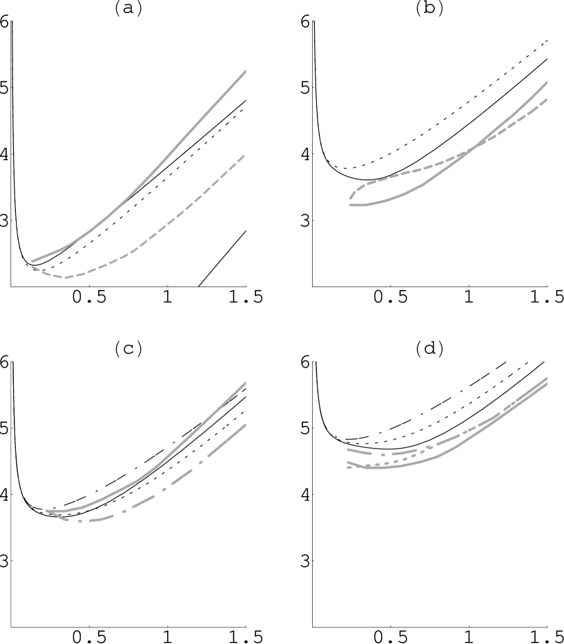
Figure 5: Hybrid potentials with corrections included (black curves) compared to lattice ones (thick grey curves) in units $1/r_{0}=$ 400 MeV ($r_{0}=2.5$ GeV^-1). $Q\bar{Q}$-distance $R$ is measured in $2r_{0}\approx$ 1 fm. States (a)–(d) are given in Table 1. Solid, dashed and dashed-dotted curves correspond to $\Lambda=1,2$ and 3. Solid line at right bottom corner of Fig.5(a) represents the Coulomb+linear potential with $\alpha_{s}=0.4$ and $\sigma=0.21$ GeV².

The results of full QCD string calculations are given at Fig.5 for the excitation curves listed in Table 1, together with the lattice data [3]. As it is seen from the Fig.5, at small distances the calculated curves are in good agreement with lattice results, with the accuracy better that 100 MeV. The level ordering is reproduced too, with the exception of $\Sigma^{-}_{g}$, $\Pi_{g}$ and $\Delta_{g}$ levels (Fig.5c). Note, that the lattice data claim only one $\Pi_{g}$ level, and its $R$-behaviour is rather peculiar (see dashed thick grey curve at Fig.5b). One expects that the curves should tend to form degenerate levels as the distance $R$ decreases, fulfilling the angular momentum conservation demands at $R=0$. This feature is made explicit in the QCD string model: our calculations reproduce the gluelump spectrum [10] for $R=0$ after subtracting the $Q\bar{Q}$ Coulomb force (last term in (19)) and with obvious replacement $2\sigma\rightarrow\sigma_{adj}=\frac{9}{4}\sigma$, $2\alpha_{s}\rightarrow\frac{9}{4}\alpha_{s}$.

Lattice data indeed seem to follow such tendency. Moreover, the curvatures of all potentials but $\Pi_{g}$ are compatible with the dominance of Coulomb force acting between static sources in octet colour representation. Thus one suspects [18], [19], that something goes wrong with the lattice $\Pi_{g}$ level, and its strange behaviour could be due to the presence of several levels, severely mixed and poorly resolved by present simulations.

The most pronounced feature of the QCD string approach is the following. It was already mentioned that the gluon here is effectively massive, and has three polarizations. As a consequence, the level ordering follows the increasing dimension of valence gluon operator, or, in other words, the increasing orbital momentum $l$. This is in contrast to the standard viewpoint of constituent glue studies, see [20] and realization of this idea in the framework of potential NRQCD [18]. The level ordering there is supposed to follow the increasing dimension of the operators $E_{i}$, $B_{i}$, $D_{i}B_{k}$ etc. The equations of motion, which relate different operators with the same quantum numbers, are involved to exclude spurios states in such picture.

In our approach, we expect an extra family of levels to appear, namely, $\Sigma^{+}_{g}$ and $\Pi_{g}$, and the corresponding gluelump limit achieved with $1^{--}$ quantum numbers. The wave functions of these states contain mostly the $l=0$ component, so these levels should be the lowest one-gluon ones. The search for this family, accessible only with electric field correlators, is of paramount importance both in gluelump and adiabatic potentials settings. The presence or absence of such states would allow to discriminate among models.

The flux-tube model [21], as well as its relativistic version [22], assumes that soft glue is string-like, with phonon-type effective degrees of freedom. These string phonons are colourless, so that the $Q\bar{Q}$ pair is in colour-singlet state. Thus the Coulomb $Q\bar{Q}$ interaction is to be attractive. Adiabatic potentials are calculated in [22], and, in order to improve the short-range behaviour of adiabatic curves, the Coulomb interquark repulsion was added, which obviously contradicts the general phylosophy of flux-tube. Without essential modifications of dynamical picture at small interquark distances, the flux-tube-type models seem to be ruled out by lattice data [3]. A rather elaborated constituent gluon model [16], based on field-theoretical Hamiltonian approach, agrees with lattice data on hybrid potentials at short and intermediate interquark distances only under rather confusing assumption of gluon parity taken to be positive.

The gluelump spectrum, as well as small $R$-limit of hybrid adiabatic potentials, is successfully calculated in the bag model [23]. The lowest bag-model gluelump state is $1^{+-}$, and the $\Sigma-\Pi$ splitting at small interquark distances is in accordance with lattice data. In this regard we stress once more the importance of lattice measurements with electric field correlators. If the ground state $\Sigma^{+}_{g}-\Pi_{g}$ family is not found, then, with above-mentioned drawbacks of flux-tube and constituent-gluon pictures, it would mean that soft glue is bag-like rather than string-like or point-like.

To conclude, we have presented full QCD string calculations of hybrid adiabatic potentials. The results are in general agreement with lattice data. We outline the problems, connected with restricted set of gluonic operators used in lattice simulations, and call for further studies of excitation curves with electric field operators.

We are grateful to Yu.A.Simonov for numerous stimulating discussions. The financial support of RFFI grants 00-02-17836 and 00-15-96786, and INTAS OPEN 2000-110, 2000-366 is acknowledged.

Appendix A Variational calculations of adiabatic potentials

In this Appendix we derive the explicit variational equations for adiabatic potentials (22).

The average momentum for oscillatory wave finction with orbital momentum $l$ is given as

$$\left<p^{2}\right>_{l}=\frac{2l+3}{2}\beta^{2},$$ (A.1)

where $\beta$ is the variational parameter with dimension of mass. Thus the calculation of extremum over $\mu$ (23) leads to expression

$$\mu^{*}=\beta\sqrt{\frac{2l+3}{2}}.$$ (A.2)

Due to the symmetry of wave functions,

$$\left<r_{1}\right>=\left<r_{2}\right>,~{}~{}\left<\frac{1}{r_{1}}\right>=\left<\frac{1}{r_{2}}\right>.$$ (A.3)

Let us introduce the dimensionless variables

$$x=\beta\,\frac{R}{2}~{}\mbox{ }~{}\tilde{r}_{1}=\beta r_{1}$$ (A.4)

and define the dimensionless averages

$$\left<\tilde{r}_{1}\right>\equiv f(x),~{}~{}\left<\frac{1}{\tilde{r}_{1}}\right>\equiv g(x).$$ (A.5)

For the energy levels we will get

$$E(\beta,x)=\frac{1}{\beta}\,2\sigma f(x)+\beta\left(\sqrt{\frac{2l+3}{2}}-3\alpha_{s}g(x)+\frac{\alpha_{s}}{12x}\right).$$

Let us perform now the extremum of the last equation over $\beta$ provided that $x$ is the function of $\beta$ and $\partial f(x(\beta))/\partial\beta=f^{\prime}(x)x/\beta$. So we find that

$$\beta^{2}(x)=\frac{2\sigma(f(x)-xf^{\prime}(x))}{\displaystyle\sqrt{\frac{2l+3}{2}}-3\alpha_{s}(g(x)+xg^{\prime}(x))},$$ (A.6)

$$E(x)=\frac{2\sigma}{\beta(x)}f(x)+\beta(x)\left(\sqrt{\frac{2l+3}{2}}-3\alpha_{s}g(x)+\frac{\alpha_{s}}{12x}\right),$$ (A.7)

$$R(x)=\frac{2x}{\beta(x)}.$$ (A.8)

The equations (A.7), (A.8), along with calculated functions $f(x),~{}g(x),~{}\beta(x)$ define explicitly adiabatic potentials (22). Note that all expressions for the averages contain the error function

$$\mathrm{erf}(x)=\frac{2}{\sqrt{\pi}}\int_{0}^{x}dt\,\mathrm{e}^{-t^{2}}.$$ (A.9)

We present them below for the levels of Table 1.

$$\rule{0.0pt}{28.45274pt}\left<\tilde{r}_{1}\right>_{110} = x\left\{\mathrm{erf}(x)\left(1+\frac{1}{x^{2}}-\frac{1}{4x^{4}}\right)+\frac{\mathrm{e}^{-x^{2}}}{\sqrt{\pi}\,x}\left(1+\frac{1}{2x^{2}}\right)\right\}$$

$$\left<\frac{1}{\tilde{r}_{1}}\right>_{110} = \frac{1}{x}\left\{\mathrm{erf}(x)\left(1-\frac{1}{2x^{2}}\right)+\frac{\mathrm{e}^{-x^{2}}}{\sqrt{\pi}\,x}\right\}$$ (A.10)

$$\beta_{110}^{2} = \frac{\displaystyle\frac{4\sigma}{x}\left\{\mathrm{erf}(x)\left(1-\frac{1}{2x^{2}}\right)+\frac{\mathrm{e}^{-x^{2}}}{\sqrt{\pi}\,x}\right\}}{\displaystyle\sqrt{\frac{5}{2}}-\frac{3\alpha_{s}}{x^{3}}\left(\mathrm{erf}(x)-\frac{2x\,\mathrm{e}^{-x^{2}}}{\sqrt{\pi}\,}\right)}$$

$$\rule{0.0pt}{45.5244pt}\left<\tilde{r}_{1}\right>_{111} = x\left\{\mathrm{erf}(x)\left(1+\frac{3}{4x^{2}}+\frac{1}{8x^{4}}\right)+\frac{\mathrm{e}^{-x^{2}}}{\sqrt{\pi}\,x}\left(1-\frac{1}{4x^{2}}\right)\right\}$$

$$\left<\frac{1}{\tilde{r}_{1}}\right>_{111} = \frac{1}{x}\left\{\mathrm{erf}(x)\left(1+\frac{1}{4x^{2}}\right)-\frac{\mathrm{e}^{-x^{2}}}{\sqrt{\pi}}\left(x+\frac{1}{2x}\right)\right\}$$ (A.11)

$$\beta_{111}^{2} = \frac{\displaystyle\frac{2\sigma}{x}\left\{\frac{1}{2}\mathrm{erf}(x)\left(3+\frac{1}{x^{2}}\right)-\frac{\mathrm{e}^{-x^{2}}}{\sqrt{\pi}}\left(x+\frac{1}{x}\right)\right\}}{\displaystyle\sqrt{\frac{5}{2}}-\frac{3\alpha_{s}}{x^{3}}\left(-\frac{1}{2}\mathrm{erf}(x)+\frac{x\,\mathrm{e}^{-x^{2}}}{\sqrt{\pi}}\left(1+2x^{2}+2x^{4}\right)\right)}$$

$$\rule{0.0pt}{45.5244pt}\left<\tilde{r}_{1}\right>_{120} = x\left\{\mathrm{erf}(x)\left(1+\frac{14}{15x^{2}}+\frac{9}{20x^{4}}\right)+\frac{\mathrm{e}^{-x^{2}}}{\sqrt{\pi}\,x}\left(\frac{11}{15}-\frac{9}{10x^{2}}\right)\right\}$$

$$\left<\frac{1}{\tilde{r}_{1}}\right>_{120} = \frac{1}{x}\left\{\mathrm{erf}(x)\left(1+\frac{7}{10x^{2}}\right)-\frac{x\,\mathrm{e}^{-x^{2}}}{5\sqrt{\pi}\,}\left(\frac{8x^{2}}{3}+\frac{28}{3}+\frac{7}{x^{2}}\right)\right\}$$ (A.12)

$$\beta_{120}^{2} = \frac{\displaystyle\frac{2\sigma}{5x}\left\{\mathrm{erf}(x)\left(\frac{28}{3}+\frac{9}{x^{2}}\right)-\frac{2\,\mathrm{e}^{-x^{2}}}{\sqrt{\pi}\,x}\left(9+\frac{22x^{2}}{3}+\frac{4x^{4}}{3}\right)\right\}}{\displaystyle\sqrt{\frac{7}{2}}-\frac{3\alpha_{s}}{5x^{3}}\left(-7\mathrm{erf}(x)+\frac{2x\,\mathrm{e}^{-x^{2}}}{\sqrt{\pi}\,}\left(7+\frac{22x^{2}}{3}+\frac{16x^{4}}{3}+\frac{8x^{6}}{3}\right)\right)}$$

$$\rule{0.0pt}{45.5244pt}\left<\tilde{r}_{1}\right>_{121} = x\left\{\mathrm{erf}(x)\left(1+\frac{77}{60x^{2}}-\frac{9}{40x^{4}}\right)+\frac{\,\mathrm{e}^{-x^{2}}}{5\sqrt{\pi}\,x}\left(\frac{14}{3}+\frac{9}{4x^{2}}\right)\right\}$$

$$\left<\frac{1}{\tilde{r}_{1}}\right>_{121} = \frac{1}{x}\left\{\mathrm{erf}(x)\left(1-\frac{7}{20x^{2}}\right)+\frac{\,\mathrm{e}^{-x^{2}}}{5\sqrt{\pi}\,}\left(\frac{7}{2x}-\frac{7x}{3}-\frac{2x^{3}}{3}\right)\right\}$$ (A.13)

$$\beta_{121}^{2} = \frac{\displaystyle\frac{2\sigma}{5x}\left\{\frac{1}{2}\mathrm{erf}(x)\left(\frac{77}{3}-\frac{9}{x^{2}}\right)+\frac{\mathrm{e}^{-x^{2}}}{\sqrt{\pi}\,x}\left(9-\frac{11x^{2}}{3}-\frac{2x^{4}}{3}\right)\right\}}{\displaystyle\sqrt{\frac{7}{2}}-\frac{3\alpha_{s}}{5x^{3}}\left(\frac{7}{2}\mathrm{erf}(x)+\frac{x\,\mathrm{e}^{-x^{2}}}{\sqrt{\pi}}\left(-7+\frac{2x^{2}}{3}+\frac{8x^{4}}{3}+\frac{4x^{6}}{3}\right)\right)}$$

$$\rule{0.0pt}{45.5244pt}\left<\tilde{r}_{1}\right>_{220} = x\left\{\mathrm{erf}(x)\left(1+\frac{1}{x^{2}}+\frac{3}{4x^{4}}-\frac{3}{2x^{6}}\right)+\frac{\mathrm{e}^{-x^{2}}}{\sqrt{\pi}\,x}\left(1+\frac{1}{2x^{2}}+\frac{3}{x^{4}}\right)\right\}$$

$$\left<\frac{1}{\tilde{r}_{1}}\right>_{220} = \frac{1}{x}\left(1+\frac{2}{x^{2}}\right)\left\{\mathrm{erf}(x)\left(1-\frac{3}{2x^{2}}\right)+\frac{3\,\mathrm{e}^{-x^{2}}}{\sqrt{\pi}\,x}\right\}$$ (A.14)

$$\beta_{220}^{2} = \frac{\displaystyle\frac{2\sigma}{x}\left\{\mathrm{erf}(x)\left(2+\frac{3}{x^{2}}-\frac{9}{x^{4}}\right)+\frac{6\,\mathrm{e}^{-x^{2}}}{\sqrt{\pi}\,x}\left(1+\frac{3}{x^{2}}\right)\right\}}{\displaystyle\sqrt{\frac{7}{2}}-\frac{3\alpha_{s}}{x^{3}}\left\{\mathrm{erf}(x)\left(-1+\frac{12}{x^{2}}\right)-\frac{2\,\mathrm{e}^{-x^{2}}}{\sqrt{\pi}\,x}\left(12+7x^{2}+2x^{4}\right)\right\}}$$

$$\rule{0.0pt}{45.5244pt}\left<\tilde{r}_{1}\right>_{221} = x\left\{\mathrm{erf}(x)\left(1+\frac{13}{12x^{2}}-\frac{1}{8x^{4}}+\frac{1}{x^{6}}\right)+\frac{\mathrm{e}^{-x^{2}}}{\sqrt{\pi}\,x}\left(\frac{2}{3}-\frac{13}{12x^{2}}-\frac{2}{x^{4}}\right)\right\}$$

$$\left<\frac{1}{\tilde{r}_{1}}\right>_{221} = \frac{1}{x}\left\{\mathrm{erf}(x)\left(1+\frac{1}{4x^{2}}+\frac{2}{x^{4}}\right)-\frac{\mathrm{e}^{-x^{2}}}{\sqrt{\pi}}\left(\frac{2x^{3}}{3}+\frac{7x}{3}+\frac{19}{6x}+\frac{4}{x^{3}}\right)\right\}$$ (A.15)

$$\beta_{221}^{2} = \frac{\displaystyle\frac{2\sigma}{x}\left\{\mathrm{erf}(x)\left(\frac{13}{6}-\frac{1}{2x^{2}}+\frac{6}{x^{4}}\right)-\frac{\mathrm{e}^{-x^{2}}}{\sqrt{\pi}}\left(\frac{2x^{3}}{3}+\frac{11x}{3}+\frac{7}{x}+\frac{12}{x^{3}}\right)\right\}}{\displaystyle\sqrt{\frac{7}{2}}-\frac{3\alpha_{s}}{x^{3}}\left\{-\mathrm{erf}(x)\left(\frac{1}{2}+\frac{8}{x^{2}}\right)+\frac{\mathrm{e}^{-x^{2}}}{\sqrt{\pi}\,x}\left(16+\frac{35x^{2}}{3}+6x^{4}+\frac{8x^{6}}{3}+\frac{4x^{8}}{3}\right)\right\}}$$

$$\rule{0.0pt}{45.5244pt}\left<\tilde{r}_{1}\right>_{222} = x\left\{\mathrm{erf}(x)\left(1+\frac{4}{3x^{2}}-\frac{1}{4x^{4}}-\frac{1}{4x^{6}}\right)+\frac{\mathrm{e}^{-x^{2}}}{\sqrt{\pi}\,x}\left(1+\frac{5}{6x^{2}}+\frac{1}{2x^{4}}\right)\right\}$$

$$\left<\frac{1}{\tilde{r}_{1}}\right>_{222} = \frac{1}{x}\left\{\mathrm{erf}(x)\left(1-\frac{1}{2x^{2}}-\frac{1}{2x^{4}}\right)+\frac{\mathrm{e}^{-x^{2}}}{\sqrt{\pi}\,x}\left(\frac{5}{3}+\frac{1}{x^{2}}\right)\right\}$$ (A.16)

$$\beta_{222}^{2} = \frac{\displaystyle\frac{2\sigma}{x}\left\{\mathrm{erf}(x)\left(\frac{8}{3}-\frac{1}{x^{2}}-\frac{3}{2x^{4}}\right)+\frac{\mathrm{e}^{-x^{2}}}{\sqrt{\pi}\,x}\left(4+\frac{3}{x^{2}}\right)\right\}}{\displaystyle\sqrt{\frac{7}{2}}-\frac{3\alpha_{s}}{x^{3}}\left\{\mathrm{erf}(x)\left(1+\frac{2}{x^{2}}\right)-\frac{2\,\mathrm{e}^{-x^{2}}}{\sqrt{\pi}\,x}\left(2+\frac{7x^{2}}{3}+\frac{2x^{4}}{3}\right)\right\}}$$

$$\rule{0.0pt}{45.5244pt}\left<\tilde{r}_{1}\right>_{230} = x\left\{\mathrm{erf}(x)\left(1+\frac{81}{70x^{2}}+\frac{33}{70x^{4}}+\frac{39}{28x^{6}}\right)-\frac{\mathrm{e}^{-x^{2}}}{\sqrt{\pi}\,x}\left(\frac{4x^{2}}{35}+\frac{1}{35}+\frac{14}{5x^{2}}+\frac{39}{14x^{4}}\right)\right\}$$

$$\left<\frac{1}{\tilde{r}_{1}}\right>_{230} = \frac{1}{x}\left\{\mathrm{erf}(x){\textstyle\left(1-\frac{36}{35x^{2}}+\frac{33}{14x^{4}}\right)}-\frac{x\,\mathrm{e}^{-x^{2}}}{\sqrt{\pi}}{\textstyle\left(\frac{33}{7x^{4}}+\frac{26}{5x^{2}}+\frac{26}{7}+\frac{44x^{2}}{35}+\frac{8x^{4}}{35}\right)}\right\}$$ (A.17)

$$\beta_{230}^{2} = \frac{\frac{2\sigma}{7x}\left\{\mathrm{erf}(x)\left(\frac{81}{5}+\frac{66}{5x^{2}}+\frac{117}{2x^{4}}\right)-\frac{\mathrm{e}^{-x^{2}}}{\sqrt{\pi}}\left(\frac{117}{x^{3}}+\frac{522}{5x}+\frac{278x}{5}+\frac{68x^{3}}{5}+\frac{8x^{5}}{5}\right)\right\}}{\frac{3}{\sqrt{2}}-\frac{3\alpha_{s}}{7x^{3}}\left\{-6\mathrm{erf}(x)\left(\frac{12}{5}+\frac{11}{x^{2}}\right)-\frac{4\,\mathrm{e}^{-x^{2}}}{\sqrt{\pi}\,x}\left(33+\frac{146x^{2}}{5}+\frac{76x^{4}}{5}+\frac{32x^{6}}{5}+\frac{12x^{8}}{5}+\frac{4x^{10}}{5}\right)\right\}}$$

$$\rule{0.0pt}{45.5244pt}\left<\tilde{r}_{1}\right>_{231} = x\left\{\mathrm{erf}(x)\left(1+\frac{93}{70x^{2}}+\frac{22}{35x^{4}}-\frac{13}{14x^{6}}\right)+\frac{\,\mathrm{e}^{-x^{2}}}{7\sqrt{\pi}\,}\left(\frac{13}{x^{5}}-\frac{2}{15x^{3}}+\frac{23}{5x}-\frac{4x}{15}\right)\right\}$$

$$\left<\frac{1}{\tilde{r}_{1}}\right>_{231} = \frac{1}{x}\left\{\mathrm{erf}(x){\textstyle\left(1+\frac{18}{35x^{2}}-\frac{11}{7x^{4}}\right)}+\frac{\,\mathrm{e}^{-x^{2}}}{7\sqrt{\pi}\,}{\textstyle\left(\frac{22}{x^{3}}+\frac{112}{15x}-\frac{98x}{15}-\frac{44x^{3}}{15}-\frac{8x^{5}}{15}\right)}\right\}$$ (A.18)

$$\beta_{231}^{2} = \frac{\frac{2\sigma}{7x}\left\{\mathrm{erf}(x)\left(\frac{93}{5}+\frac{88}{5x^{2}}-\frac{39}{x^{4}}\right)-\frac{4\,\mathrm{e}^{-x^{2}}}{\sqrt{\pi}\,}\left(\frac{39}{2x^{3}}+\frac{21}{5x}-\frac{107x}{30}-\frac{17x^{3}}{15}-\frac{2x^{5}}{15}\right)\right\}}{\frac{3}{\sqrt{2}}-\frac{12\alpha_{s}}{7x^{3}}\left\{\mathrm{erf}(x)\left(-\frac{9}{5}+\frac{11}{x^{2}}\right)+\frac{2\,\mathrm{e}^{-x^{2}}}{\sqrt{\pi}\,x}\left(-11-\frac{83x^{2}}{15}-\frac{14x^{4}}{15}+\frac{8x^{6}}{15}+\frac{2x^{8}}{5}+\frac{2x^{10}}{15}\right)\right\}}$$

$$\rule{0.0pt}{45.5244pt}\left<\tilde{r}_{1}\right>_{232} = x\left\{\mathrm{erf}(x)\left(1+\frac{129}{70x^{2}}-\frac{121}{140x^{4}}+\frac{13}{56x^{6}}\right)+\frac{\mathrm{e}^{-x^{2}}}{\sqrt{\pi}\,x}\left(1+\frac{149}{105x^{2}}-\frac{13}{28x^{4}}\right)\right\}$$

$$\left<\frac{1}{\tilde{r}_{1}}\right>_{232} = \frac{1}{x}\left\{\mathrm{erf}(x)\left(1-\frac{36}{35x^{2}}+\frac{11}{28x^{4}}\right)+\frac{\mathrm{e}^{-x^{2}}}{\sqrt{\pi}}\left(-\frac{11}{14x^{3}}+\frac{23}{15x}+\frac{8x}{105}\right)\right\}$$ (A.19)

$$\beta_{232}^{2} = \frac{\displaystyle\frac{2\sigma}{7x}\left\{\mathrm{erf}(x)\left(\frac{129}{5}-\frac{121}{5x^{2}}+\frac{39}{4x^{4}}\right)+\frac{\mathrm{e}^{-x^{2}}}{\sqrt{\pi}}\left(-\frac{39}{2x^{3}}+\frac{177}{5x}+\frac{16x}{15}\right)\right\}}{\displaystyle\frac{3}{\sqrt{2}}-\frac{6\alpha_{s}}{7x^{3}}\left\{\mathrm{erf}(x)\left(\frac{36}{5}-\frac{11}{2x^{2}}\right)+\frac{\mathrm{e}^{-x^{2}}}{\sqrt{\pi}\,x}\left(11-\frac{106x^{2}}{15}-\frac{52x^{4}}{15}-\frac{8x^{6}}{15}\right)\right\}}$$

Appendix B String corrections

The string correction potentials, $V^{\mathrm{sc}}_{jl\Lambda}=\left<\vec{\Psi}_{jl\Lambda}|H^{\mathrm{sc}}|\vec{\Psi}_{jl\Lambda}\right>$, have the following form:

$$V^{\mathrm{sc}}_{110} = -\frac{4\sigma x}{15\beta}\left\{\mathrm{erf}(x)\left(1+\frac{2}{x^{2}}-\frac{11}{4x^{4}}\right)+\frac{\mathrm{e}^{-x^{2}}}{\sqrt{\pi}\,x}\left(1+\frac{11}{2x^{2}}\right)\right\},$$ (B.1)

$$V^{\mathrm{sc}}_{111} = -\frac{\sigma x}{15\beta}\left\{3\mathrm{erf}(x)\left(1+\frac{3}{2x^{2}}-\frac{13}{6x^{4}}\right)+\frac{\mathrm{e}^{-x^{2}}}{\sqrt{\pi}\,x}\left(5+\frac{13}{x^{2}}\right)\right\},$$ (B.2)

$$V^{\mathrm{sc}}_{120} = -\frac{2\sigma x}{105\beta}\left\{\mathrm{erf}(x)\left(\frac{28}{3}+\frac{67}{3x^{2}}-\frac{3}{2x^{4}}\right)+\right.$$ (B.3)

$$\left.+\frac{\mathrm{e}^{-x^{2}}}{\sqrt{\pi}}\left(\frac{3}{x^{3}}-\frac{32}{3x}-16x-\frac{16x^{3}}{3}\right)\right\},$$

$$V^{\mathrm{sc}}_{121} = -\frac{2\sigma x}{210\beta}\left\{\mathrm{erf}(x)\left(\frac{77}{3}+\frac{139}{6x^{2}}+\frac{3}{2x^{4}}\right)+\right.$$ (B.4)

$$\left.+\frac{\mathrm{e}^{-x^{2}}}{\sqrt{\pi}}\left(-\frac{3}{x^{3}}+\frac{47}{3x}-8x-\frac{8x^{3}}{3}\right)\right\},$$

$$V^{\mathrm{sc}}_{220} = -\frac{2\sigma x}{21\beta}\left\{\mathrm{erf}(x)\left(2+\frac{2}{x^{2}}-\frac{3}{2x^{4}}+\frac{9}{2x^{6}}\right)+\frac{\mathrm{e}^{-x^{2}}}{\sqrt{\pi}}\left(-\frac{9}{x^{5}}-\frac{3}{x^{3}}+\frac{2}{x}\right)\right\},$$ (B.5)

$$V^{\mathrm{sc}}_{221} = -\frac{2\sigma x}{21\beta}\left\{\mathrm{erf}(x)\left(\frac{13}{6}+\frac{59}{12x^{2}}+\frac{3}{4x^{4}}-\frac{3}{x^{6}}\right)+\right.$$ (B.6)

$$\left.+\frac{\mathrm{e}^{-x^{2}}}{\sqrt{\pi}}\left(\frac{6}{x^{5}}+\frac{5}{2x^{3}}-\frac{17}{6x}-4x-\frac{4x^{3}}{3}\right)\right\},$$

$$V^{\mathrm{sc}}_{222} = -\frac{2\sigma x}{21\beta}\left\{\mathrm{erf}(x)\left(\frac{8}{3}+\frac{5}{3x^{2}}+\frac{3}{4x^{6}}\right)+\frac{\mathrm{e}^{-x^{2}}}{\sqrt{\pi}}\left(-\frac{3}{2x^{5}}-\frac{1}{x^{3}}+\frac{8}{3x}\right)\right\},$$ (B.7)

$$V^{\mathrm{sc}}_{230} = -\frac{2\sigma x}{27\beta}\left\{\mathrm{erf}(x)\left(\frac{81}{35}+\frac{237}{70x^{2}}+\frac{87}{70x^{4}}-\frac{9}{4x^{6}}\right)+\right.$$ (B.8)

$$\left.+\frac{\mathrm{e}^{-x^{2}}}{\sqrt{\pi}\,x}\left(\frac{9}{2x^{4}}+\frac{18}{35x^{2}}+\frac{131}{35}+\frac{8x^{2}}{7}+\frac{8x^{4}}{35}\right)\right\},$$

$$V^{\mathrm{sc}}_{231} = -\frac{2\sigma x}{27\beta}\left\{\mathrm{erf}(x)\left(\frac{93}{35}+\frac{277}{70x^{2}}-\frac{1}{5x^{4}}+\frac{3}{2x^{6}}\right)+\right.$$ (B.9)

$$\left.+\frac{\mathrm{e}^{-x^{2}}}{\sqrt{\pi}\,x}\left(-\frac{3}{x^{4}}-\frac{8}{5x^{2}}+\frac{53}{21}+\frac{8x^{2}}{2}1+\frac{8x^{4}}{105}\right)\right\},$$

$$V^{\mathrm{sc}}_{232} = -\frac{2\sigma x}{27\beta}\left\{\mathrm{erf}(x)\left(\frac{129}{35}+\frac{41}{10x^{2}}-\frac{59}{140x^{4}}-\frac{3}{8x^{6}}\right)+\right.$$ (B.10)

$$\left.+\frac{\mathrm{e}^{-x^{2}}}{\sqrt{\pi}\,x}\left(\frac{3}{4x^{4}}+\frac{47}{35x^{2}}+\frac{53}{15}\right)\right\}.$$

Appendix C Spin-orbit corrections

Nonperturbative spin-orbit potentials, given as $V^{\mathrm{LS}\,(\mathrm{np})}_{jl\Lambda}=\left<\vec{\Psi}_{jl\Lambda}|H^{\mathrm{LS}\,(\mathrm{np})}|\vec{\Psi}_{jl\Lambda}\right>$, are

$$V^{\mathrm{LS}\,(\mathrm{np})}_{110} = \frac{2\sigma}{5\beta x}\left\{\mathrm{erf}(x)\left(1-\frac{1}{2x^{2}}\right)+\frac{\mathrm{e}^{-x^{2}}}{\sqrt{\pi}\,x}\right\},$$ (C.1)

$$V^{\mathrm{LS}\,(\mathrm{np})}_{111} = \frac{\sigma}{5\beta x}\left\{\mathrm{erf}(x)\left(1+\frac{1}{2x^{2}}\right)-\frac{\mathrm{e}^{-x^{2}}}{\sqrt{\pi}\,x}\right\},$$ (C.2)

$$V^{\mathrm{LS}\,(\mathrm{np})}_{120} = \frac{18\sigma}{35\beta x}\left\{\mathrm{erf}(x)\left(1+\frac{1}{2x^{2}}\right)-\frac{\mathrm{e}^{-x^{2}}}{\sqrt{\pi}\,x}\left(1+\frac{8x^{2}}{9}\right)\right\},$$ (C.3)

$$V^{\mathrm{LS}\,(\mathrm{np})}_{121} = \frac{3\sigma}{35\beta x}\left\{\mathrm{erf}(x)\left(7-\frac{3}{2x^{2}}\right)+\frac{\mathrm{e}^{-x^{2}}}{\sqrt{\pi}\,x}\left(3-\frac{4x^{2}}{3}\right)\right\},$$ (C.4)

$$V^{\mathrm{LS}\,(\mathrm{np})}_{220} = \frac{2\sigma}{7\beta x}\left(1+\frac{2}{x^{2}}\right)\left\{\mathrm{erf}(x)\left(1-\frac{3}{2x^{2}}\right)+\frac{3\,\mathrm{e}^{-x^{2}}}{\sqrt{\pi}\,x}\right\},$$ (C.5)

$$V^{\mathrm{LS}\,(\mathrm{np})}_{221} = \frac{2\sigma}{7\beta x}\left\{\mathrm{erf}(x)\left(\frac{2}{3}-\frac{1}{2x^{2}}+\frac{2}{x^{4}}\right)-\frac{x\,\mathrm{e}^{-x^{2}}}{\sqrt{\pi}}\left(\frac{2}{3}+\frac{5}{3x^{2}}+\frac{4}{x^{4}}\right)\right\},$$ (C.6)

$$V^{\mathrm{LS}\,(\mathrm{np})}_{222} = \frac{2\sigma}{7\beta x}\left\{\mathrm{erf}(x)\left(\frac{1}{3}+\frac{1}{2x^{2}}-\frac{1}{2x^{4}}\right)+\frac{\mathrm{e}^{-x^{2}}}{\sqrt{\pi}\,x}\left(-\frac{1}{3}+\frac{1}{x^{2}}\right)\right\},$$ (C.7)

$$V^{\mathrm{LS}\,(\mathrm{np})}_{230} = \frac{2\sigma}{63\beta x}\left\{{\textstyle\mathrm{erf}(x)\left(16+\frac{54}{5x^{2}}+\frac{21}{x^{4}}\right)}-\frac{4\,\mathrm{e}^{-x^{2}}}{\sqrt{\pi}\,}{\textstyle\left(\frac{21}{4x^{3}}+\frac{31}{5x}+4x+\frac{4x^{3}}{5}\right)}\right\},$$ (C.8)

$$V^{\mathrm{LS}\,(\mathrm{np})}_{231} = \frac{4\sigma}{9\beta x}\left\{\mathrm{erf}(x)\left(\frac{26}{21}+\frac{3}{5x^{2}}-\frac{1}{x^{4}}\right)+\right.$$ (C.9)

$$\left.+\frac{2\,\mathrm{e}^{-x^{2}}}{\sqrt{\pi}\,}\left(\frac{1}{x^{3}}+\frac{1}{15x}-\frac{16x}{35}-\frac{8x^{3}}{105}\right)\right\},$$

$$V^{\mathrm{LS}\,(\mathrm{np})}_{232} = \frac{2\sigma}{9\beta x}\left\{{\textstyle\mathrm{erf}(x)\left(\frac{64}{21}-\frac{69}{35x^{2}}+\frac{1}{2x^{4}}\right)}+\frac{\mathrm{e}^{-x^{2}}}{\sqrt{\pi}}{\textstyle\left(-\frac{1}{x^{3}}+\frac{344}{105x}-\frac{8x}{105}\right)}\right\}.$$ (C.10)

Perturbative spin-dependent potentials, $V^{\mathrm{LS}\,(\mathrm{p})}_{jl\Lambda}=\left<\vec{\Psi}_{jl\Lambda}|H^{\mathrm{LS}\,(\mathrm{p})}|\vec{\Psi}_{jl\Lambda}\right>$, read as

$$V^{\mathrm{LS}\,(\mathrm{p})}_{110} = -\frac{3\alpha_{s}\beta}{5x^{3}}\left\{\mathrm{erf}(x)+\frac{2x\,\mathrm{e}^{-x^{2}}}{\sqrt{\pi}\,}\right\},$$ (C.11)

$$V^{\mathrm{LS}\,(\mathrm{p})}_{111} = \frac{3}{5}\alpha_{s}\beta\left\{\frac{\mathrm{erf}(x)}{2x^{3}}-\frac{\mathrm{e}^{-x^{2}}}{\sqrt{\pi}}\left(2+\frac{1}{x^{2}}\right)\right\},$$ (C.12)

$$V^{\mathrm{LS}\,(\mathrm{p})}_{120} = \frac{3}{7}\alpha_{s}\beta\left\{\frac{3\mathrm{erf}(x)}{5x^{3}}-\frac{2\,\mathrm{e}^{-x^{2}}}{5\sqrt{\pi}\,}\left(6+\frac{3}{x^{2}}+8x^{2}\right)\right\},$$ (C.13)

$$V^{\mathrm{LS}\,(\mathrm{p})}_{121} = -\frac{3}{7}\alpha_{s}\beta\left\{\frac{3\mathrm{erf}(x)}{10x^{3}}+\frac{\,\mathrm{e}^{-x^{2}}}{5\sqrt{\pi}\,}\left(6-\frac{3}{x^{2}}+4x^{2}\right)\right\},$$ (C.14)

$$V^{\mathrm{LS}\,(\mathrm{p})}_{220} = \frac{3}{7}\alpha_{s}\beta\left\{-\frac{\mathrm{erf}(x)}{x^{3}}\left(1+\frac{6}{x^{2}}\right)+\frac{2\,\mathrm{e}^{-x^{2}}}{\sqrt{\pi}\,}\left(2+\frac{5}{x^{2}}+\frac{6}{x^{4}}\right)\right\},$$ (C.15)

$$V^{\mathrm{LS}\,(\mathrm{p})}_{221} = \frac{3}{7}\alpha_{s}\beta\left\{\frac{4\mathrm{erf}(x)}{x^{5}}-\frac{4\,\mathrm{e}^{-x^{2}}}{3\sqrt{\pi}\,}\left(2+\frac{5}{x^{4}}+\frac{4}{x^{2}}+x^{2}\right)\right\},$$ (C.16)

$$V^{\mathrm{LS}\,(\mathrm{p})}_{222} = \frac{3}{7}\alpha_{s}\beta\left\{\frac{\mathrm{erf}(x)}{x^{3}}\left(1-\frac{1}{x^{2}}\right)-\frac{\mathrm{e}^{-x^{2}}}{\sqrt{\pi}}\left(\frac{4}{3}+\frac{2}{3x^{2}}-\frac{2}{x^{4}}\right)\right\},$$ (C.17)

$$V^{\mathrm{LS}\,(\mathrm{p})}_{230} = \frac{8}{21}\alpha_{s}\beta\left\{\frac{\mathrm{erf}(x)}{x^{3}}\left(1+\frac{9}{4x^{2}}\right)-\frac{\mathrm{e}^{-x^{2}}}{\sqrt{\pi}}\left(\frac{18}{5}+\frac{9}{2x^{4}}+\frac{5}{x^{2}}+\frac{12x^{2}}{5}+\frac{8x^{4}}{5}\right)\right\},$$ (C.18)

$$V^{\mathrm{LS}\,(\mathrm{p})}_{231} = \frac{4}{21}\alpha_{s}\beta\left\{\frac{\mathrm{erf}(x)}{x^{3}}\left(1-\frac{3}{x^{2}}\right)+\frac{2\,\mathrm{e}^{-x^{2}}}{\sqrt{\pi}\,}\left(-\frac{14}{15}+\frac{3}{x^{4}}+\frac{1}{x^{2}}-\frac{4x^{2}}{3}-\frac{8x^{4}}{15}\right)\right\},$$ (C.19)

$$V^{\mathrm{LS}\,(\mathrm{p})}_{232} = \frac{2}{21}\alpha_{s}\beta\left\{\frac{\mathrm{erf}(x)}{x^{3}}\left(-4+\frac{3}{2x^{2}}\right)+\frac{\mathrm{e}^{-x^{2}}}{\sqrt{\pi}}\left(\frac{4}{15}-\frac{3}{x^{4}}+\frac{6}{x^{2}}-\frac{8x^{2}}{15}\right)\right\}.$$ (C.20)

References

• [1] A.Donnachie ans Yu.S.Kalashnikova, Phys.Rev. D60, 114011 (1999)
• [2] M.Foster and C.Michael, Phys.Rev. D59, 094509 (1999)
• [3] K.J.Juge, J.Kuti and C.J.Morningstar, in Proc. LATTICE 98, Nucl.Phys.Proc.Suppl. 73, 590 (1999)
K.J.Juge, J.Kuti and C.J.Morningstar, Phys.Rev.Lett. 82, 4400 (1999)
K.J.Juge, J.Kuti and C.Morningstar, hep-lat/0103008
• [4] Yu.A. Simonov, Lectures at the XVII Int. School of Physics, Lisbon (1999), hep-ph/9911237
• [5] A.Di Giacomo, H.G.Dosch, V.I.Shevchenko, Yu.A.Simonov, hep-ph/0007223
• [6] A.Yu.Dubin, A.B.Kaidalov and Yu.A.Simonov, Phys.Lett. B323, 41 (1994)
• [7] V.L.Morgunov, A.V.Nefediev and Yu.A.Simonov, Phys.Lett. B459, 653 (1999)
Yu.S.Kalashnikova and A.V.Nefediev, Phys.Lett. B492, 91 (2000)
Yu.S.Kalashnikova, A.V.Nefediev and Yu.A.Simonov, Phys.Rev. D64, 014037 (2001)
A.M.Badalian, B.L.G.Bakker, hep-ph/0202246
• [8] A.B.Kaidalov and Yu.A.Simonov, Phys.Atom.Nucl. 63, 1428 (2000)
A.B.Kaidalov and Yu.A.Simonov, Phys.Lett B477, 163 (2000)
• [9] Yu.A.Simonov Nucl.Phys.B (proc. Suppl) 23, 283 (1990)
Yu.S.Kalashnikova, Yu.B.Yufryakov, Phys.Lett. B359, 175 (1995)
Yu.S.Kalashnikova, Yu.B.Yufryakov, Phys.Atom.Nucl. 60, 307 (1997)
• [10] Yu.A.Simonov, Nucl.Phys. B592, 350 (2001)
• [11] Yu.A.Simonov, Phys.Atom.Nucl. 64, 1876 (2001)
• [12] Yu.S.Kalashnikova, D.S.Kuzmenko, Phys.Atom.Nucl. 64, 1716 (2001)
• [13] Yu.A.Simonov, Phys.Atom.Nucl. 58, 107 (1995)
• [14] Yu.S.Kalashnikova and A.V.Nefediev, Phys.Atom.Nucl. 60, 1389 (1997)
Yu.S.Kalashnikova and A.V.Nefediev, Phys.Atom.Nucl. 61, 785 (1998
• [15] D.Horn and J.Mandula, Phys.Rev. D17, 898 (1978)
• [16] E.S.Swanson and A.P.Szczepaniak, Phys.Rev. D59, 014035 (1999)
• [17] Yu.A.Simonov, Nucl.Phys. B324, 67 (1989)
A.M.Badalian and Yu.A.Simonov, Phys.Atom.Nucl. 59, 2164 (1996)
• [18] N.Brambilla, A.Pineda, J.Soto, A.Vairo, Nucl.Phys. B566, 275 (2000)
• [19] G.S.Bali, Phys.Rept. 343, 1 (2001)
• [20] R.L.Jaffe, K.Johnson and Z.Ryzak, Ann.Phys. 168, 344 (1986)
• [21] N.Isgur and J.Paton, Phys.Rev. D31, 2910 (1985)
• [22] T.J.Allen, M.G.Olsson, S.Veseli, Phys.Lett. B434, 110 (1998)
• [23] G.Karl and J.Paton, Phys.Rev. D60, 034015 (1999)