Instantons and $\langle A^{2}\rangle$ Condensate

Abstract

We argue that the $<A_{\rm OPE}^{2}>$ condensate found in the Landau gauge on lattices, when an Operator Product Expansion of Green functions is performed, might be explained by instantons. We use cooling to estimate the instanton contribution and extrapolate back the result to the thermalised configuration. The resulting $<A_{\rm inst}^{2}>$ is similar to $<A_{\rm OPE}^{2}>$.

I Introduction

Lattice calculations of the gluon propagator and three-point Green function in the Landau gauge indicate that the expected perturbative behaviour at large momentum $p$ has to be corrected by a $O(1/p^{2})$ contribution sizeable up to 10 GeV [1, 2, 3, 4, 5]. An understanding of this contribution as the effect of an $A^{2}\equiv A_{\mu}^{a}A_{a}^{\mu}$ condensate (in the Landau gauge $A^{2}$ is the only mass dimension-two operator liable to have a v.e.v.) has been gained by verifying that two independent Green functions could be described by the perturbative contribution corrected by the effect of one common value of $<A^{2}_{\rm OPE}>$, as expected from OPE. The physical origin of this condensate is an important question, possibly involving the non-trivial topology of the QCD vacuum. In particular, instantons provide an interesting insight into a wide range of low energy QCD properties ([6] and refs therein). They have been put into evidence on the lattice using different cooling procedures. In this letter we claim that instantons provide for $<A^{2}>$ a value close to what is needed for the OPE fit to Green functions.

We propose a method to identify instantons from the cooled gauge configuration, count them and measure their radii; we also check that these results are compatible with the instanton number deduced from the two-point correlation function of an instanton. We then estimate $<A_{\rm inst}^{2}>$, the contribution of the instantons to $<A^{2}>$ in cooled configurations, extrapolate back to the thermalised configurations (zero cooling sweeps) and finally, compare the outcome with the OPE estimate.

II Cooling and instanton counting by shape recognition

A cooling

In order to study the influence of the underlying classical properties of a given lattice configuration, the first step will be to isolate these structures from UV modes. The method we use is due to Teper [7]; it consists in replacing each link by a unitary matrix proportional to the staple. A cooling sweep is performed after replacing all the links of the lattice. This procedure introduces largely discussed biases, such as UV instanton disappearance and instanton–anti-instanton pair annihilations, that increase with the number of cooling sweeps; alternative cooling methods have been proposed (see for example [8] and refs. therein) to cure these diseases. We will try to reduce them by identifying the instantons after a few cooling sweeps and extrapolating back to the thermalised gauge configuration.

B Instantons

Instantons (anti-instantons) are classical solutions [9] of the equations of motion. We work in the Landau gauge which is defined on the lattice by minimizing $\sum_{x}A_{\mu}(x)^{2}$. For an instanton solution this prescription leads to the singular Landau gauge, where the gauge field is[9]

$$A^{(I)a}_{\mu}=\frac{2\overline{\eta}^{a}_{\mu\nu}x_{\nu}\rho^{2}}{x^{2}\left(x^{2}+\rho^{2}\right)}\ ,$$ (1)

$\rho$ being the instanton radius. The instanton has been chosen centered at the origin with a conventional color orientation. These solutions have $Q=\pm 1$ topological charge,

$$Q\equiv\frac{g^{2}}{32\pi^{2}}\int d^{4}xF^{\mu\nu}_{a}\widetilde{F}^{a}_{\mu\nu}=\pm\frac{g^{2}}{32\pi^{2}}\int d^{4}xF^{\mu\nu}_{a}{F}^{a}_{\mu\nu}\ ,$$ (2)

where $\widetilde{F}_{\mu\nu}=\frac{1}{2}\epsilon_{\mu\nu\rho\sigma}F^{\rho\sigma}$. From eq. (1) the topological charge density is:

$$Q_{\rho}(x)=\pm\frac{6}{\pi^{2}\rho^{4}}\left(\frac{\rho^{2}}{x^{2}+\rho^{2}}\right)^{4}\ ,$$ (3)

On the lattice, the topological charge density will be computed as

$$Q_{\rm latt}(x)\ =\ \frac{1}{2^{9}\pi^{2}}\sum_{\pm 1}^{\pm 4}\widetilde{\epsilon}_{\mu\nu\rho\sigma}Tr[\Pi_{\mu\nu}(x)\Pi_{\rho\sigma}(x)]\ ,$$ (4)

with $\Pi_{\mu\nu}(x)=U_{\mu}(x)U_{\nu}(x+\mu\hat{a})U^{\dagger}_{\mu}(x+\mu\hat{a}+\nu\hat{a})U^{\dagger}_{\nu}(x+\nu\hat{a})$, and $\widetilde{\epsilon}_{\mu\nu\rho\sigma}$ the antisymmetric tensor, with an extra minus sign for each negative index.

C identification of instantons

A common belief is that an instanton liquid gives a fair description of important features of the QCD vacuum. Along this line we will try a desciption of our cooled gauge configuration as an ensemble of non-interacting instantons with random positions and color orientations. We hence also neglect the interaction-induced instanton deformations and correlations. Although the instanton ensemble for the QCD vacuum cannot be considered as a dilute gas [6, 7, 8, 9, 10, 11, 12], this crude assumption allows a qualitatively reasonable picture, especially near the instanton center.

Many enlightening works have studied the instanton properties from lattice gauge configurations, among which [13, 14, 15, 16]. As for us, we start by searching regions where the topological charge density looks like that of Eq.(3). Starting from each local maximum or minimum of $Q_{\rm latt}(x)$ we integrate over all neighbouring points with $|Q_{\rm latt}(x)|\geq\alpha|Q_{\rm latt}(x_{max})|$, for different values of $\alpha$ ranging from $0.8$ to $0.4$. A local extremum is accepted to be an (anti-)instanton if the ratio $\epsilon$ between the lattice integral and its theoretical counterpart, $Q_{\rho}(x)$,

$$\epsilon\ =\ \left(1-3\alpha^{1/2}+2\alpha^{3/4}\right)^{-1}\ \int_{{x}/\ |Q({x})|\geq\alpha|Q(0)|}d^{4}x\ Q_{\rm latt}(x)$$ (5)

shows a plateau when $\alpha$ is varied. Indeed for a theoretical (anti-)instanton $\epsilon=1$ ($\epsilon=-1$) for any $\alpha\in[0,1]$. As a cross-check of self-duality, this instanton shape recognition (ISR) procedure is applied on the lattice to both expressions for $Q$ introduced in eq. (2).

D Instanton numbers and radii

The ISR method resolves the semiclassical structure on the lattice with only $\sim 5$ cooling sweeps. This early recognition reduces the possible cooling-induced bias.

Whenever this method succeeds, we measure the radius of the accepted instanton in two separate ways: from the maximum value of $Q$, written $Q_{\rm latt}^{\rm max}$, at the center of the instanton, and from the number $N_{\alpha}$ of lattice points in the volume $\int_{{x}/\ |Q({x})|\geq\alpha|Q(0)|}d^{4}x$. We find:

$$\rho/a\ =\sqrt[4]{\frac{6}{\pi^{2}Q_{\rm latt}^{\rm max}}}=\frac{1}{\sqrt{\alpha^{-1/4}-1}}\sqrt[4]{\frac{2N_{\alpha}}{\pi^{2}}}\ ,$$ (6)

These two measures of the radius agree within $10\%$.

III gluon propagator

A The instanton gauge-field correlation function

The classical gauge-field two-point correlation function verifies, for any position and color orientation,

$$\frac{1}{8}\sum_{a}\overline{G}_{\mu\nu}^{aa}\ \equiv\frac{1}{8V}\sum_{a}\left(A^{(I)a}_{\mu}(k)A^{(I)a}_{\nu}(-k)\right)\ =\overline{G}^{(2)}(k^{2})\ \left(\delta_{\mu\nu}-\frac{k_{\mu}k_{\nu}}{k^{2}}\right)\ \ ,$$ (7)

where $V$ is the volume in the euclidean four-dimensional space and $A^{(I)a}_{\mu}(k)$ is the Fourier Transform of Eq.(1). The resulting scalar form factor is:

$$\overline{G}^{(2)}(k^{2})\ =\ \frac{32\pi^{4}}{Vk^{6}}\left(1-\frac{(k\rho)^{2}}{2}K_{2}(k\rho)\right)^{2}\ ,$$ (8)

$K_{2}$ being a Bessel function [17]. Eq. (8) equally applies to instantons and anti-instantons.

In a perfect gas approximation for an ensemble of $n_{I}$ ($n_{A}$) (anti-)instantons of radius $\rho$, the classical gauge-field correlation function is simply given by Eq.(8) times the number of instantons and anti-instantons, $n_{I}+n_{A}$. This correlation function is the contribution of the background field to the gluon propagator. We expect this formula to describe the behaviour of the lattice gluon propagator once the effect of quantum UV fluctuations is removed by the cooling procedure [7]. The effect of instanton interactions is known [10, 11] to modify the instanton shape far from its center, in the IR region. But the large $k^{2}$ behaviour should be appropriately given by Eq.(8) i.e. $\propto 1/k^{6}$. This is shown in Fig.1.a for one generic lattice gauge field configuration.

The theoretical lines in that plot are generated by Eq.(8) using the average radius $\rho$ and $n_{I}+n_{A}$ computed from the ISR method. Note that the matching improves with the number of cooling sweeps. This agrees with the expectation that decreasing the instanton density reduces the instanton deformation and that quantum fluctuations are damped by cooling. Reversely, if we know the average radius from the ISR method, we can compute $n_{I}+n_{A}$ from the fit to the measured propagator.

B The hard gluon propagator

Let us now consider a hard gluon of momentum $p_{\mu}$ propagating in an instanton gas background. The gluon interacts with the instanton gauge field. This can be computed with Feynman graphs and it is easy to see that when the instanton modes $k_{\mu}$ verifies $k_{\mu}\sim 1/\rho\ll p_{\mu}$, the dominant contribution is an $O(1/p^{2})$ correction to the perturbative gluon. This correction is equal to the standard OPE Wilson coefficient [2, 3] times $<A^{2}_{\rm inst}(0)>\equiv 1/V\int d^{4}x\left(A^{(I)}\right)^{2}(x)$. We will now proceed to estimate this instanton-induced condensate.

IV $<A^{2}>$ condensate

A $<A^{2}>$ in instantons

From Eq.(1) we get

$$<A_{\rm inst}^{2}(n_{c})>\equiv\frac{n_{I}+n_{A}}{V}\ \int d^{4}x\sum_{\mu,a}A^{(I)a}_{\mu}A^{(I)a}_{\mu}\ =\ 12\pi^{2}\rho^{2}\frac{n_{I}+n_{A}}{V}\ .$$ (9)

where $\rho$ is the average instanton radius in the considered cooled configuration and $n_{c}$ is the number of cooling sweeps.

We use an ensemble of 10 independent gauge configurations at $\beta=6.0$ on a $24^{4}$ lattice. Each configuration has been cooled and after 5,7,10,15,30 and 100 cooling sweeps transformed into the Landau gauge. Using the ISR method on each gauge configuration, we obtain the results of Tab.I. In this table we also present the number of (anti-)instantons and the corresponding value for $<A^{2}(n_{c})>$ computed by a Correlation Function Fit (CFF) i.e. a fit of the lattice propagators to the instanton correlation function, Eq.(8). The CFF method is expected to be affected differently from the ISR method by systematic uncertainties: instanton interactions, deformations and quantum fluctuations (as we can see in Fig.1.a, at low momentum), and we therefore consider as quite encouraging the qualitative agreement - becoming quantitative at large $n_{c}$ - between ISR and CFF results. We have, for simplicity, translated our lattice results into physical units using, for all values of $n_{c}$, the $n_{c}=0$ inverse lattice spacing, $a^{-1}(n_{c}=0)=1.996$ GeV (at $\beta=6.0$). This simple recipe overlooks the effect of cooling on the lattice spacing (see ref. [15] and refs. therein) but this simplification becomes harmless after extrapolating back our results to $n_{c}=0$.

B $<A_{\rm inst}^{2}(n_{c})>$ at zero cooling.

The instanton number depends on the number of cooling sweeps. This result may imply that the cooling procedure destroys not only quantum UV fluctuations but something else from the semiclassical background of gauge fields. To lessen this problem we take advantage of the early recognition of the instanton content in a gauge configuration ensured by the ISR method and perform an extrapolation [19] to $n_{c}=0$ of the ISR results for $<A^{2}_{\rm inst}(n_{c})>$ in the table. We then obtain (see fig.1.b):

$$<A^{2}_{\rm inst}(n_{c}=0)>=1.76(23)\;{\rm GeV}^{2}\ .$$ (10)

We have used a form $a/(b+n_{c})$ to fit and extrapolate. We have also varied a little this functional form to check the stability of the extrapolation. We take this result as indicative of the non-perturbative instanton contribution to the $<A^{2}>$ condensate. If we applied other lattice estimates of instanton gas parameters taken from the available literature to Eq.(9), the value of $<A^{(I)^{2}}>$ would range  from 1 to 2 GeV². On the other hand, parameters from instanton liquid based phenomenology[6] yield estimates of the order of 0.5 GeV². As the quoted error in Eq.(10) is only statistical, this last range somehow estimates a certain systematic uncertainty.

$n_{c}$	$\rho$ (fm)	$n_{I}+n_{A}$	$<A^{2}>$  (GeV2)
5 7 10 15 30 100	ISR 0.329(2) 0.361(2) 0.394(4) 0.417(5) 0.452(9) 0.53(1)	ISR CFF 87(2) 93(10) 74(2) 59(1) 60(1) 38(1) 43(1) 28(1) 26(1) 19(1) 10(1) 9(1)	ISR CFF 1.38(3) 0.9(8) 1.42(5) 1.12(2) 1.36(4) 0.86(2) 1.11(4) 0.72(2) 0.80(6) 0.57(3) 0.43(3) 0.37(3)

TABLE I.: Estimates of $<A^{2}_{\rm inst}(n_{c})>$.

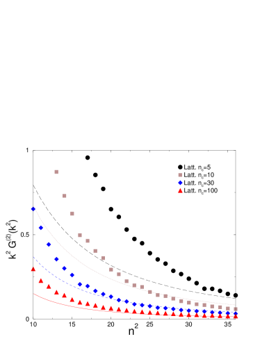
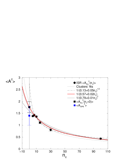
FIG. 1.: In fig. (a) (left) we present the lattice gluon propagators after several number of cooling sweeps (points) and the corresponding theoretical instanton gauge-field correlation functions (lines) in the perfect instanton gas approximation, Eq.(8), plotted as a function of $n^{2}$ ($n_{\mu}\equiv L/(2\pi)\ k_{\mu}$, $L$ being the lattice length). In fig. (b) (right), we show the extrapolation at zero cooling of $<A^{2}(n_{c})>$ in physical units (for three different trial functions).

C Comparison with $<A^{2}>$ from OPE.

Our instanton estimate of $\langle A^{2}\rangle$ is a semiclassical one, deprived of the necessary UV fluctuations, and therefore not directly comparable with [2] $\langle A^{2}_{\rm OPE}\rangle(10{\rm GeV})=2.4(5)~{}$GeV². There is of course no exact recipe to compare both estimates, since the separation between the semiclassical non perturbative domain and the perturbative one cannot be exact. We may appeal to the fact that at the renormalisation point $\mu$, the radiative corrections are minimised; therefore a semiclassical estimate must best correspond to $\langle A^{2}_{\rm OPE}\rangle$ at some reasonable $\mu$. In the example of $\phi^{2}$ vacuum expectation in the spontaneously broken $\phi^{4}$ model given in [21], one finds indeed that it equals the classical estimate for $\mu$ around the spontaneously generated mass. In our problem, one could guess that the corresponding scale should typically be around $1/\rho\simeq 0.7$ GeV, or some gluonic mass, a very low scale anyway. We cannot run $\langle A^{2}_{\rm OPE}\rangle(10{\rm GeV})$ down to such a low scale [2],

$$A^{2}_{R,\mu}=A^{2}_{R,\mu_{0}}\ \left(1+\frac{35}{44}\ \ln{\frac{\mu}{\mu_{0}}}\ /\ \ln{\frac{\mu}{\Lambda_{\rm MOM}}}\right)\ .$$ (11)

we therefore stop arbitrarily $\mu\sim 2.6$ GeV, where the OPE corrected perturbative running of the Green functions fails to correctly describe their behaviour. This scale of 2.6 GeV turns out to be of the same order[2] as the critical mass[22] for the gluon propagator. At this scale, we obtain:

$$<A^{2}_{\rm OPE}(2.6\ {\rm GeV})>=1.4(3)(3)\;{\rm GeV}^{2}\ ,$$ (12)

where the first quoted error just propagates the uncertainty from the OPE determination of $<A^{2}>$ and the second one takes into account, in the way proposed in ref. [4], higher orders in $\alpha_{s}$ for running.

V Discussion and conclusions

We are aware that our method of comparison of $<A^{2}_{\rm inst}(n_{c}=0)>$ and $<A^{2}_{\rm OPE}>$ suffers from a lot of arbitrariness and approximations (such as the perfect gas approximation, possible errors in the instanton identification, the uncertainty in the extrapolation to zero cooling sweeps, etc.). We have taken care to crosscheck our estimates by comparing different methods at each step of the computation, in particular the ISR and CFF (see Fig.1.a and Tab. I). A comparison with direct “measurements” of the $\langle A^{2}\rangle$ condensate from cooled lattice configurations could be thought as an additional crosscheck. Qualitative agreement is found for a large enough number of cooling sweeps, but this agreement is manifestly destroyed by UV fluctuations already for $n_{c}\sim 30$. Of course, by using ISR and instanton gas approximation we sharply separate UV fluctuations from the semiclassical background. All these imprecisions seem anyway inherent to the subject.

With this in mind, we nevertheless take the fair agreement between Eqs. (10) and (12) as a convincing indication that the $A^{2}$ condensate receives a significant instantonic contribution. In other words, the instanton liquid picture might yield the explanation for the $1/p^{2}$ corrections to the perturbative behaviour of Green functions computed with thermalised configurations on the lattice.

REFERENCES

- [1] Ph. Boucaud et al., JHEP 0004, 006 (2000) [arXiv:hep-ph/0003020].
- [2] Ph. Boucaud, A. Le Yaouanc, J. P. Leroy, J. Micheli, O. Pene and J. Rodriguez-Quintero, Phys. Lett. B 493, 315 (2000) [arXiv:hep-ph/0008043].
- [3] Ph. Boucaud, A. Le Yaouanc, J. P. Leroy, J. Micheli, O. Pene and J. Rodriguez-Quintero, Phys. Rev. D 63, 114003 (2001) [arXiv:hep-ph/0101302].
- [4] D. Becirevic, Ph. Boucaud, J. P. Leroy, J. Micheli, O. Pene, J. Rodriguez-Quintero and C. Roiesnel, Phys. Rev. D 60, 094509 (1999). Phys. Rev. D 61, 114508 (2000);
- [5] F. De Soto and J. Rodriguez-Quintero, Phys. Rev. D 64, 114003 (2001) [arXiv:hep-ph/0105063].
- [6] T. Schafer and E. V. Shuryak, Rev. Mod. Phys. 70 (1998) 323.
- [7] M. Teper, Phys. Lett. B 162, 357 (1985); Phys. Lett. B 171 (1986) 86.
- [8] M. Garcia Perez, O. Philipsen and I. O. Stamatescu, Nucl. Phys. B 551, 293 (1999) [arXiv:hep-lat/9812006].
- [9] G. ’t Hooft, Phys. Rev. D 14 (1976) 3432 [Erratum-ibid. D 18 (1976) 2199].
- [10] D. Diakonov and V. Y. Petrov, Nucl. Phys. B 245 (1984) 259.
- [11] J. J. Verbaarschot, Nucl. Phys. B 362 (1991) 33 [Erratum-ibid. B 386 (1991) 236].
- [12] M. Hutter, arXiv:hep-ph/0107098.
- [13] M. C. Chu, J. M. Grandy, S. Huang and J. W. Negele, Phys. Rev. D 49, 6039 (1994) [arXiv:hep-lat/9312071].
- [14] P. de Forcrand, M. Garcia Perez and I. O. Stamatescu, Nucl. Phys. B 499, 409 (1997) [arXiv:hep-lat/9701012].
- [15] D. A. Smith and M. J. Teper [UKQCD collaboration], Phys. Rev. D 58 (1998) 014505; [arXiv:hep-lat/9801008].
- [16] C. Michael and P. S. Spencer, Phys. Rev. D 52, 4691 (1995);
- [17] I.S. Gradshteyn, I.M. Ryzhiz, ”Table of Integrals, Series, and Products” (5th edition) Academic Press (1994).
- [18] W. Broniowski, private communication.
- [19] J. W. Negele, Nucl. Phys. Proc. Suppl. 73, 92 (1999) [arXiv:hep-lat/9810053].
- [20] P. de Forcrand, M. García Pérez, J. E. Hetrick, I-O. Stamatescu, in “31st International Symposium Ahrenshoop on the Theory of Elementary Particles, Buckow, September 2-6, 1997” [arXiv:hep-lat/9802017]
- [21] V. A. Novikov, M.A. Shifman, A.I. Vainshtein, V.I. Zakharov, Nucl. Phys. B249 (1985) 445;
- [22] V. A. Novikov, M. A. Shifman, A. I. Vainshtein and V. I. Zakharov, Nucl. Phys. B 191, 301 (1981).
- [23]