Photonuclear interaction of high energy muons and tau-leptons

E.V. Bugaev, Yu.V. Shlepin

Institute for Nuclear Research, the Academy of Sciences of Russia, Moscow, Russia

Abstract General formalism for the two-component description of the inelastic lepton-nucleon scattering in the diffractive region is proposed. Nonperturbative contribution to electromagnetic structure functions of a nucleon is described by the modified generalized vector dominance model containing special cut-off factors restricting the phase volume of the initial $\stackrel{{\scriptstyle\,~{}-}}{{qq}}$-pairs of virtual photon’s fluctuations. Perturbative QCD contribution is described by the phenomenological model suggested (in nonunitarized form) by Forshaw, Kerley and Shaw.

Formulae needed for a numerical calculation of photonuclear cross sections integrated over $Q^{2}$ are presented. It is argued that in the case of the photonuclear cross sections at superhigh energies of leptons ($E\gtrsim 10^{5}GeV$), integrated over $Q^{2}$, the following two-component scheme is good enough: the nonperturbative contribution is approximated by the old parameterization of Bezrukov and Bugaev, and perturbative one is described by the model of Forshaw, Kerley and Shaw with parameters determined from DESY data. Corresponding results of numerical calculations of the perturbative part, for the cases of $\mu A$ and $\tau A$ scattering at superhigh energies, are given.

PACS number(s): 13.60.-r, 12.40.Vv

1.Introduction

The photonuclear interaction of leptons is , by definition, the process of the inelastic lepton-nucleon or lepton-nucleus scattering,

$$l+N~{}\to~{}l+(hadrons).$$

This process goes through a virtual photon exchange. In the particular case when the four-momentum transferred from the lepton to hadrons is large ($\sqrt{-q^{2}}>>1GeV$) the process (1.1) is called the deep inelastic scattering; we are interested in the present work in the diffractive region of the kinematic variables (any $q^{2}\leqslant 0$, transferred energy $\nu(=-q_{0})$ is large, such that $x_{Bj}\sim q^{2}/2q_{0}$ is small). This region is especially important for applications in cosmic ray physics and neutrino astrophysics. The typical problem requiring a knowledge of the photonuclear cross section is the study of muon and tau propagation through thick layers of matter [1]. High energy muons produced in collisions of cosmic primaries in atmosphere (the process is $Z_{CR}+Z_{Atm}\to\pi\to\mu$) are detected and studied by modern large underground (and underwater) telescopes. As for taus, they can be produced in the Earth by extragalactic high energy $\tau-$neutrinos (such neutrinos must always present in an extragalactic neutrino flux, due to $\nu_{\mu}\longleftrightarrow\nu_{\tau}$ oscillations).

The process (1.1) is reduced to the absorption of the virtual photon by the nucleon,

$$\gamma^{\ast}+N\to(hadrons),$$

and, by optical theorem, is connected with the Compton scattering of a virtual photon,

$$\gamma^{\ast}+N\to\gamma^{\ast}+N.$$

The Compton scattering in the diffractive region is described by the vacuum exchange which, in turn, is modelled in QCD by the exchange of two or more gluons in a colour singlet state. It becomes possible because, in laboratory system, the interaction region has a large longitudinal size, and the photon developes an internal structure due to its coupling to quark fields. In the diffractive region, i.e. at small $x_{Bj}$, the diffractive $\gamma^{\ast}N-$scattering is dominant in the Compton amplitude, as compared to the direct contribution due to a photon’s bare component (although, the direct process cannot be neglected absolutely, especially at high energies of leptons).

These general statements (about diffractive, hadron-like, nature of $\gamma^{\ast}N-$ interaction and even about the two-gluon exchange) are not enough for a quantitative calculation of the Compton amplitude or $\gamma^{\ast}N$ total cross section. One must know also the photon wave function or, by other words, the spectrum of hadron-like constituents of the photon and, besides, the amplitudes of the scattering of these constituents on a nucleon. In pre-QCD era these problems were considered, almost exclusively, in terms of vector dominance models. These models use a hadronic basis for a description of the spectrum of photon’s constituents. It is well known, however, that they can describe the main features of the $\gamma^{\ast}N-$interaction (e.g., the Bjorken scaling) only by using rather unnatural assumptions on hadronic amplitudes (see, e.g., [2]). With advent of QCD it became clear that the description of the photon wave function in terms of purely hadronic constituents is not consistent: the $\stackrel{{\scriptstyle\,~{}-}}{{qq}}$-component interacting with a target perturbatively must be added. Such a picture arises due to inherent QCD properties (asymptotic freedom, colour transparency).

The aim of the present work is twofold. In the first part of the work we formulate the two-component model of the electromagnetic structure functions of a nucleon separating, in the general form, the nonperturbative part which is described by a generalized vector dominance model. The difference with previous works on the subject [3,4] consists just in the use in our approach the generalized vector dominance, without limiting oneself by low-mass vector mesons ($\rho,\omega,\phi$) only. At the second part of the work we consider the perturbative component and carry out the concrete calculations of photonuclear cross sections for leptons of superhigh energies.

The paper is organized as follows. In sec.2 the general formulas for the two-component structure functions are derived. The hard (nonperturbative) component of the structure functions is considered, in a framework of the colour dipole model, in Sec.3. In Sec.4. we show how the existing widely used formula [5] for the photonuclear cross section must be modified to take into account the contribution of the hard component. Results of numerical calculations and conclusions are presented in the last section.

2.Two-component model of structure functions

A.Two-step picture of the Compton scattering

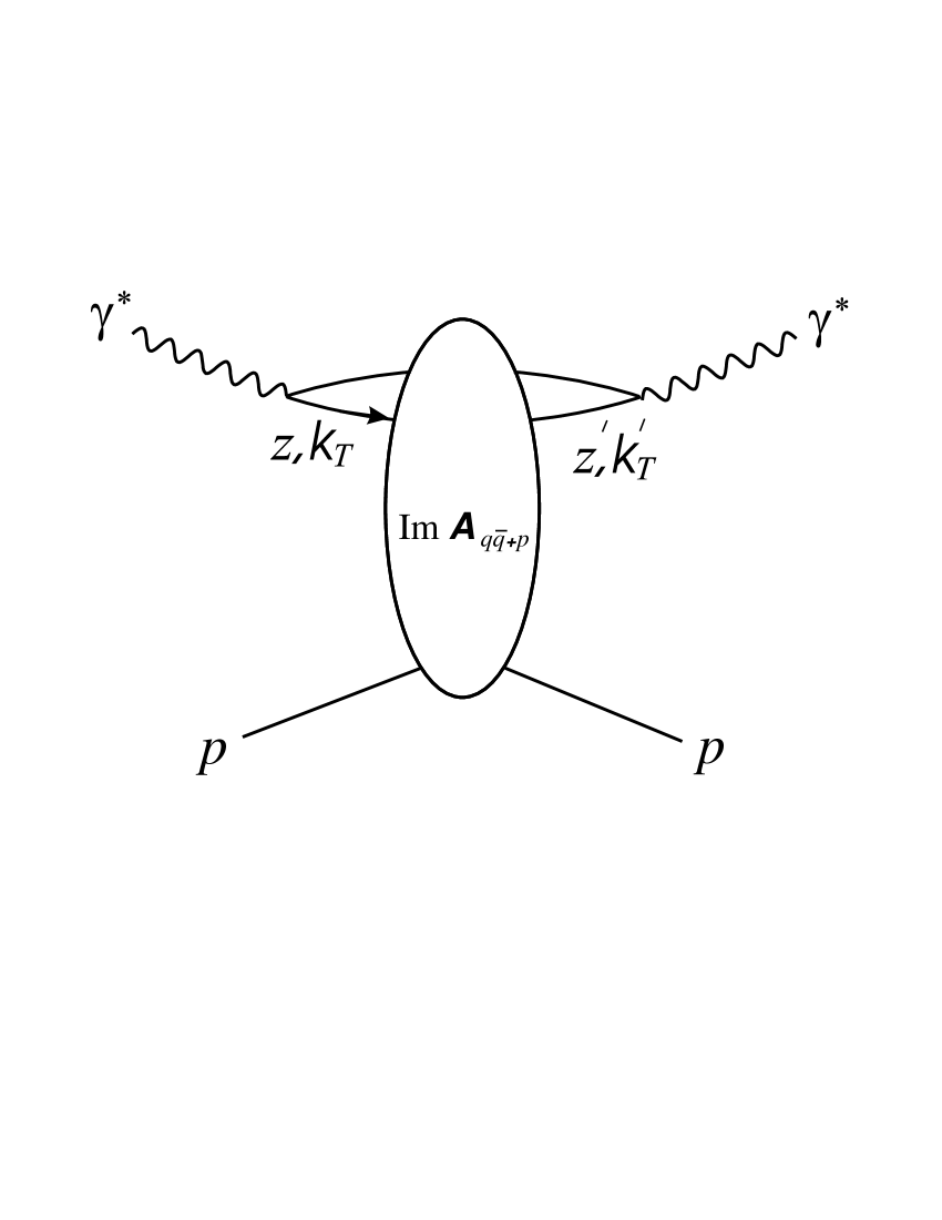
Figure 1: The diagram representing schematically the contribution of $\stackrel{{\scriptstyle\,~{}-}}{{qq}}$-channel in the imaginary part of the Compton forward scattering amplitude.

The starting point of our consideration is the expression based on the perturbative QCD and the two-step picture of the $\gamma^{\ast}p$ interaction: the first step is the $\gamma^{\ast}\rightarrow\stackrel{{\scriptstyle\,~{}-}}{{qq}}$ conversion, and the second step is an interaction of the $\stackrel{{\scriptstyle\,~{}-}}{{qq}}$-pair with the target proton. The total $\gamma^{\ast}p$ interaction cross section ( summed over all possible final hadronic states) is given by the contribution of the $\stackrel{{\scriptstyle\,~{}-}}{{qq}}$-channel in the imaginary part of the Compton forward scattering amplitude ( fig.1):

$$\sigma_{T,L}(Q^{2},s)=\frac{1}{16\pi^{3}}\sum\limits_{f}\sum\limits_{r,r^{\prime}}\int dz\int d^{2}k_{\bot}\int dz^{\prime}\int d^{2}k^{\prime}_{\bot}\times$$

$$\times{\psi^{T,L}_{\gamma(r,r^{\prime})}}^{\ast}(\stackrel{{\scriptstyle\to}}{{k}}^{\prime}_{\bot},z^{\prime},Q^{2})\frac{1}{s}\mathcal{A}_{\stackrel{{\scriptstyle\,~{}-}}{{qq}}+p}(\stackrel{{\scriptstyle\to}}{{k}}^{\prime}_{\bot},z^{\prime},\stackrel{{\scriptstyle\to}}{{k}}_{\bot},z;s)\psi^{T,L}_{\gamma(r,r^{\prime})}(\stackrel{{\scriptstyle\to}}{{k}}_{\bot},z,Q^{2}).$$

In this expression $\mathcal{A}_{\stackrel{{\scriptstyle\,~{}-}}{{qq}}+p}$ is the imaginary part of the $(\stackrel{{\scriptstyle\,~{}-}}{{qq}})p$ forward scattering amplitude, $Q^{2}$ and $\sqrt{s}$ are a virtuality of the photon and a $\gamma^{\ast}p$ center-of-mass energy, $\psi_{\gamma(r,r^{\prime})}$ is the light cone wave function of $\stackrel{{\scriptstyle\,~{}-}}{{qq}}$-fluctuations of a virtual photon with transverse or longitudinal polarization. This wave function depends on quark and antiquark helicities $(r,r^{\prime})$, quark mass $(m_{f})$ and quark momentum variables $z,k_{\bot}$ ($z=k_{+}/q_{+}$ is the fraction of the photon light cone momentum carried by the quark, $k_{\bot}$ is the transverse momentum of the incoming quark). In the following we will need the expressions for the squares of these wave functions summed over the quark helicities:

$$\sum\limits_{r,r^{\prime}}{\psi^{T}_{\gamma(r,r^{\prime})}}^{\ast}(\stackrel{{\scriptstyle\to}}{{k}}^{\prime}_{\bot},z,Q^{2})\psi^{T}_{\gamma(r,r^{\prime})}(\stackrel{{\scriptstyle\to}}{{k_{\bot}}},z,Q^{2})=2N_{c}\frac{e_{f}^{2}(\stackrel{{\scriptstyle\to}}{{k^{\prime}_{\bot}}}\stackrel{{\scriptstyle\to}}{{k_{\bot}}}[z^{2}+{(1-z)}^{2}]+m_{f}^{2})}{(M^{2}+Q^{2})({M^{\prime}}^{2}+Q^{2})z^{2}{(1-z)}^{2}},$$

$$\sum\limits_{r,r^{\prime}}{\psi^{L}_{\gamma(r,r^{\prime})}}^{\ast}(\stackrel{{\scriptstyle\to}}{{k}}^{\prime}_{\bot},z,Q^{2})\psi^{L}_{\gamma(r,r^{\prime})}(\stackrel{{\scriptstyle\to}}{{k_{\bot}}},z,Q^{2})=8N_{c}\frac{e_{f}^{2}Q^{2}}{(M^{2}+Q^{2})({M^{\prime}}^{2}+Q^{2})}.$$

In these formulas $M$ and $M^{\prime}$ are invariant masses of the incoming and outcoming $\stackrel{{\scriptstyle\,~{}-}}{{qq}}$-pairs,

$$M^{2}=\frac{k_{\bot}^{2}+m^{2}_{f}}{z(1-z)},~{}~{}{M^{\prime}}^{2}=\frac{{k^{\prime}}^{2}_{\bot}+m^{2}_{f}}{z(1-z)}.$$

B.Two gluon exchange approximation

We suppose, further, that the forward scattering amplitude in Eq.(2.1) can be written in the form

$$\frac{1}{s}\mathcal{A}_{\stackrel{{\scriptstyle\,~{}-}}{{qq}}+p}(\stackrel{{\scriptstyle\to}}{{k}}^{\prime}_{\bot},z^{\prime},\stackrel{{\scriptstyle\to}}{{k}}_{\bot},z;s)=\{\delta(\stackrel{{\scriptstyle\to}}{{k}}^{\prime}_{\bot}-\stackrel{{\scriptstyle\to}}{{k_{\bot}}})\int d^{2}l^{\prime}_{\bot}B({l^{\prime}}^{2}_{\bot},s)-B(l^{2}_{\bot},s)\}\delta(z^{\prime}-z),$$

$$\stackrel{{\scriptstyle\to}}{{l}}_{\bot}=\stackrel{{\scriptstyle\to}}{{k}}^{\prime}_{\bot}-\stackrel{{\scriptstyle\to}}{{k_{\bot}}}.$$

Such a form of the $(\stackrel{{\scriptstyle\,~{}-}}{{qq}})p$ amplitude is suggested by the model of the structure functions [6] based on the two-gluon exchange approximation of perturbative QCD [7-10]. The first term in Eq.(2.4) corresponds to the diagonal transition when $M^{2}={M^{\prime}}^{2}$; the delta-function factor in this term arises due to zero transverse momentum transfer to the quark ( at high energies the value of $z$ is frozen during the scattering process, and the interaction can, in a general case, change only the transverse momentum of $\stackrel{{\scriptstyle\,~{}-}}{{qq}}$ pair’s particles ). In the case of nondiagonal transitions ( the second term in Eq.(2.4)) the scattering amplitude depends on the square of the transverse momentum, $\stackrel{{\scriptstyle\to}}{{l}}_{\bot}=\stackrel{{\scriptstyle\to}}{{k}}^{\prime}_{\bot}-\stackrel{{\scriptstyle\to}}{{k_{\bot}}}$, transferred to the quark.

In spite of the fact that the expressions (2.1), (2.4) are based on the perturbation theory, they can be used for an approximated calculation of the photoabsorption cross section and electromagnetic structure functions of a nucleon at low $Q^{2}$, where nonperturbative effects are important. It is assumed in such an approach that the perturbative fluctuation of the $\gamma^{\ast}$ into a $\stackrel{{\scriptstyle\,~{}-}}{{qq}}$ pair is the dominant process and the subsequent colour singlet exchange is realized by two gluons only. The problem of the inclusion of higher Fock states (i.e., $\stackrel{{\scriptstyle\,~{}-}}{{qq}}g$ ) in the photon wave function was discussed in the third work of ref.[6]. As for the two-gluon exchange appoximation for a description of the elastic $(\stackrel{{\scriptstyle\,~{}-}}{{qq}})p$ - amplitude, the nonperturbative effects are approximately taken into account by introducing an effective mass of the gluons and an effective quark-gluon coupling constant. The description of soft hadronic processes via the exchange of two effective gluons was suggested many years ago in the works [7,8].

Below we will use the simple ansatz for the function $B(l^{2}_{\bot},s)$ at small $l^{2}_{\bot}$:

$$B(l^{2}_{\bot},s)=\frac{\sigma_{0}(s)}{l^{2}_{\bot}}.$$

The $l_{\bot}$ dependence of this type is obtained in the models of refs.[6-10] if, in addition to the two-gluon exchange, a constituent quark model of the target nucleon is used. More exactly, in this case one has [6]

$$B(l^{2}_{\bot},s)=\frac{V(\stackrel{{\scriptstyle\to}}{{l_{\bot}}})}{{(l^{2}_{\bot}+\mu_{G})}^{2}},$$

where $V(\stackrel{{\scriptstyle\to}}{{l_{\bot}}})$ is the GGNN-vertex function,

$$V(\stackrel{{\scriptstyle\to}}{{l_{\bot}}})\cong 1-e^{-\frac{l^{2}_{\bot}}{2<r^{2}_{N}>}},$$

$\mu_{G}$ is the effective mass of the gluon, $<r^{2}_{N}>$ is the mean square radius of a nucleon. If $\mu_{G}$ is small, there is the region,

$$\mu^{2}_{G}<<l^{2}_{\bot}\stackrel{{\scriptstyle<}}{{~{}}}\frac{1}{<r^{2}_{N}>},$$

in which $B(l^{2}_{\bot},s)\sim 1/l^{2}_{\bot}$, as in Eq.(2.5).

In purely perturbative QCD (colour dipole picture of the interaction [6,10-12], leading $\alpha_{s}ln\frac{1}{x}$ approximation) one obtains for the $B(l^{2}_{\bot},s)$ function:

$$B(l^{2}_{\bot},s)\cong\frac{4\pi}{3}f(x^{\prime},l^{2}_{\bot})\alpha_{s}(l^{2}_{\bot})\frac{1}{l^{4}_{\bot}},$$

$$x^{\prime}=\frac{Q^{2}+M^{2}}{s}.$$

Here, $f(x,l^{2}_{\bot})$ is the unintegrated gluon distribution in a proton. One can conclude, comparing Eqs.(2.5) and (2.9), that the ansatz(2.5) is not justified by the perturbative QCD calculation.

C.Separation of perturbative and nonperturbative parts

Below, in this section, we use the general expressions (2.1-2.4) for a separation of soft (nonperturbative) and hard (perturbative) contributions in the structure functions.

A nature of the $(\stackrel{{\scriptstyle\,~{}-}}{{qq}})p$ interaction is connected with a transverse size of the $\stackrel{{\scriptstyle\,~{}-}}{{qq}}$-pair: only for a small $r_{\bot}$ this nature is, due to the asymptotic freedom, perturbative while the pairs with a large enough $r_{\bot}$ interact nonperturbatively. An average transverse separation between particles of the pair is

$$\stackrel{{\scriptstyle-}}{{r}}_{\bot}=v_{\bot,relative}\tau,$$

where $v_{\bot,relative}$ is an relative velocity in the transverse direction,

$$v_{\bot,relative}=\frac{1}{2}(\frac{k_{\bot}}{E}+\frac{k_{\bot}}{E^{\prime}}),$$

$$E=\sqrt{zk_{\gamma}+k^{2}_{\bot}+m^{2}_{f}},~{}E^{\prime}=\sqrt{(1-z)k_{\gamma}+k^{2}_{\bot}+m^{2}_{f}},$$

and $\tau$ is the lifetime of the $\stackrel{{\scriptstyle\,~{}-}}{{qq}}$-fluctuation,

$$\tau=\frac{1}{\sqrt{k^{2}_{\gamma}+M^{2}}-\sqrt{k^{2}_{\gamma}-Q^{2}}}\cong\frac{2k_{\gamma}}{M^{2}+Q^{2}},$$

where $k_{\gamma}$ is the virtual photon’s three-momentum.

If follows from Eqs.(2.10-2.12) that

$$\stackrel{{\scriptstyle-}}{{r}}_{\bot}\cong\frac{1}{k_{\bot}(1+\frac{Q^{2}}{M^{2}})}.$$

We use the following criterion of the nonperturbative nature of the interaction: the $(\stackrel{{\scriptstyle\,~{}-}}{{qq}})p$ interaction is nonperturbative if

$$\stackrel{{\scriptstyle-}}{{r}}_{\bot}\geqslant r_{\bot 0}\equiv\frac{1}{k_{\bot 0}},$$

where $k_{\bot 0}$ is some parameter. This criterion, together with Eqs.(2.3) (where the approximation $m_{f}=0$ is used) and Eq.(2.13), leads to the corresponding constraint for the variable $z$,

$$z(1-z)\leqslant\frac{k^{2}_{\bot 0}M^{2}}{(M^{2}+Q^{2})^{2}}=\begin{cases}\frac{k^{2}_{\bot 0}}{M^{2}},~{}Q^{2}<<M^{2}\\ ~{}~{}~{}~{}~{}~{}~{}~{}~{}~{}~{}~{}~{}~{}~{}~{}~{}~{}~{}~{}~{}\\ \frac{k^{2}_{\bot 0}M^{2}}{Q^{4}},~{}Q^{2}>>M^{2},\end{cases}$$

according to which the $(\stackrel{{\scriptstyle\,~{}-}}{{qq}})p$ interaction is nonperturbative if the $\stackrel{{\scriptstyle\,~{}-}}{{qq}}$-pair is asymmetric [13], i.e., $E\ll E^{\prime}$ or $E^{\prime}\ll E$. In turn, the high degree of asymmetry corresponds (in accordance with Eqs.(2.3)), at a given value of $M$, to a small $k_{\bot}$ of pair’s particles and to their alignment in the direction of the virtual photon (the ”aligned jet” conjecture had been suggested in the work [14]).

D.Hard component

It is convenient, for considering the structure functions in the perturbative domain, to use the impact parameter representation. The resulting formula for $\sigma_{T,L}(Q^{2},s)$, which follows from Eqs.(2.1-2.4), is well known [6]:

$$\sigma_{T,L}(Q^{2},s)=\int dz\int d^{2}r_{\bot}\sigma(r_{\bot},s){\mid\psi^{T,L}_{\gamma}(\stackrel{{\scriptstyle\to}}{{r}}_{\bot},z,Q^{2})\mid}^{2}.$$

The squares of the photon wave functions in impact parameter space summed over helicities are given by the expressions

$$\mid\psi^{T}_{\gamma}(r_{\bot},z,Q^{2})\mid^{2}=\frac{3\alpha}{2\pi^{2}}\sum\limits_{f}{(\frac{e_{f}}{e})}^{2}\{[z^{2}+{(1-z)}^{2}]\stackrel{{\scriptstyle-~{}}}{{Q^{2}}}K^{2}_{1}(\stackrel{{\scriptstyle-}}{{Q}}r_{\bot})+m^{2}_{f}K^{2}_{0}(\stackrel{{\scriptstyle-}}{{Q}}r_{\bot})\},$$

$$\mid\psi^{L}_{\gamma}(r_{\bot},z,Q^{2})\mid^{2}=\frac{3\alpha}{2\pi^{2}}\sum\limits_{f}{(\frac{e_{f}}{e})}^{2}4z^{2}{(1-z)}^{2}Q^{2}K^{2}_{0}(\stackrel{{\scriptstyle-}}{{Q}}r_{\bot})\},$$

$$\stackrel{{\scriptstyle-~{}}}{{Q^{2}}}\equiv Q^{2}z(1-z)+m^{2}_{f}.$$

The factor $\sigma(r_{\bot},s)$ in Eq.(2.15) is a total cross section of the interaction of the $\stackrel{{\scriptstyle\,~{}-}}{{qq}}$-pair of the transverse size $r_{\bot}$ with a target proton,

$$\sigma(r_{\bot},s)=\int d^{2}l_{\bot}(1-e^{-i\stackrel{{\scriptstyle\to}}{{l}}_{\bot}\stackrel{{\scriptstyle\to}}{{r}}_{\bot}})B(l^{2}_{\bot},s).$$

Using Eq.(2.9) for $B(l^{2}_{\bot},s)$, one obtains (for small values of $r_{\bot}$)

$$\sigma(r_{\bot},s)\approx\frac{\pi^{2}}{3}r^{2}_{\bot}\alpha_{s}(\frac{1}{r^{2}_{\bot}})x^{\prime}_{eff}G(x^{\prime}_{eff},\frac{1}{r^{2}_{\bot}}),$$

where $xG(x,Q^{2})$ is the gluon structure function of a proton. Approximately one has

$$x^{\prime}_{eff}\approx\frac{{(k^{2}_{\bot})}_{eff}}{s}\sim\frac{1}{r^{2}_{\bot}s},$$

and[12]

$$\sigma(r_{\bot},s)\approx\frac{\pi^{2}}{3}r^{2}_{\bot}\alpha_{s}(\frac{1}{r^{2}_{\bot}}){[xG(x,\frac{1}{r^{2}_{\bot}})]}_{x=\frac{1}{r^{2}_{\bot}s}}.$$

Below we will use, instead of Eq.(2.20), the phenomenological model [15] for $\sigma(r_{\bot},s)$, containing except the colour transparency factor $r^{2}_{\bot}$ also the cut-off factor at large $r_{\bot}$ (which is necessary for a separation of the perturbative part of the structure functions). In such models one has

$$\sigma(r_{\bot},s)\sim r^{2}_{\bot}e^{-\frac{r_{\bot}}{r^{0}_{\bot}}}(r^{2}_{\bot}s)^{\lambda_{H}}.$$

Note, that $s$-variable enters the r.h.s. of Eq.(2.21) in combination with $r_{\bot}^{2}$ only, i.e., in the same manner as in the formula (2.20) obtained in perturbative QCD.

E.Soft component

For considering the nonperturbative part of $\sigma_{T,L}(Q^{2},s)$ we rewrite Eq.(2.1) in a form of the double dispersion relation. For this aim we perform the following change of variables:

$$\int dz\int d^{2}k_{\bot}\int d^{2}k^{\prime}_{\bot}=$$

$$=\pi\int dzz^{2}(1-z)^{2}\int dM^{2}\int d{M^{\prime}}^{2}\int\frac{{dl^{\ast}_{\bot}}^{2}}{2MM^{\prime}\sqrt{1-cos^{2}\phi}},$$

$$cos^{2}\phi=\frac{1}{4M^{2}{M^{\prime}}^{2}}(M^{2}+{M^{\prime}}^{2}-{l^{\ast}_{\bot}}^{2}),$$

$${l^{\ast}_{\bot}}^{2}\equiv\frac{l^{2}_{\bot}}{z(1-z)},~{}~{}~{}~{}~{}~{}~{}~{}(M-M^{\prime})^{2}\leq{l^{\ast}_{\bot}}^{2}\leq(M+M^{\prime})^{2}.$$

Using this change of variables and the expressions (2.2) for the squares of the photon wave functions we have, instead of Eq.(2.1),

$$\sigma_{T,L}(Q^{2},s)=\sum\limits_{f}\int\frac{dM^{2}}{M^{2}+Q^{2}}\times$$

$$\times\int\frac{d{M^{\prime}}^{2}}{{M^{\prime}}^{2}+Q^{2}}\int dz\rho_{T,L}(z)\frac{1}{s}ImA^{T,L}_{\stackrel{{\scriptstyle\,~{}-}}{{qq}}+p}(M^{2},{M^{\prime}}^{2},s),$$

$$\rho_{T}(z)=\frac{3}{2}[z^{2}+(1-z)^{2}],$$

$$\rho_{L}(z)=\frac{3}{2}4z(1-z).$$

The functions $\rho_{T,L}(z)$ are normalized densities of $\stackrel{{\scriptstyle\,~{}-}}{{qq}}$ states in the $z$-space. Imaginary parts of the forward $(\stackrel{{\scriptstyle\,~{}-}}{{qq}})p$ scattering amplitudes $A^{T,L}_{\stackrel{{\scriptstyle\,~{}-}}{{qq}}+p}(M^{2},{M^{\prime}}^{2},s)$ are obtained using Eqs.(2.4,2.5):

$$\frac{1}{s}ImA^{T}_{\stackrel{{\scriptstyle\,~{}-}}{{qq}}+p}(M^{2},{M^{\prime}}^{2},s)=\frac{1}{12\pi^{2}}N_{c}e^{2}_{f}\{M^{2}\delta(M^{2}-{M^{\prime}}^{2})[\int d^{2}l^{\prime}_{\bot}B({l^{\prime}}^{2}_{\bot},s)]-$$

$$-\int\frac{d{l^{\ast}_{\bot}}^{2}}{2\sqrt{1-cos^{2}\phi}}B({l^{\ast}_{\bot}}^{2},s)\},$$

$$\frac{1}{s}ImA^{L}_{\stackrel{{\scriptstyle\,~{}-}}{{qq}}+p}(M^{2},{M^{\prime}}^{2},s)=\frac{Q^{2}}{MM^{\prime}}\frac{1}{s}ImA^{T}_{\stackrel{{\scriptstyle\,~{}-}}{{qq}}+p}(M^{2},{M^{\prime}}^{2},s).$$

For convenience we included the factor $\frac{Q^{2}}{MM^{\prime}}$ in the definition of a longitudinal $(\stackrel{{\scriptstyle\,~{}-}}{{qq}})p$ amplitude $A_{L}$.

It is important to underline that for the derivation of Eqs.(2.23-2.24) the expression (2.5) for the function $B(l^{2}_{\bot},s)$ was used. The factorization of a $z$-dependence and the simple form of this dependence given by the functions of Eqs.(2.23a,b) became possible just due to the assumption that $B(l_{\bot}^{2},s)\sim l_{\bot}^{-2}$. The use of this assumption is leqitimate if we consider the nonperturbative component of the structure functions.

Now, for the separation of the nonperturbative contribution in the double dispersion relation (2.23) one must take into account the restriction of the $\stackrel{{\scriptstyle\,~{}-}}{{qq}}$ pair’s phase space due to the constraint (2.14a). After such a restriction the nonperturbative part of $\sigma_{T,L}(Q^{2},s)$ can be written in the form

$$\sigma_{T,L}(Q^{2},s)=\sum\limits_{f}\int\frac{dM^{2}}{M^{2}+Q^{2}}\times$$

$$\times\int\frac{d{M^{\prime}}^{2}}{{M^{\prime}}^{2}+Q^{2}}\eta_{T,L}(M^{2},{M^{\prime}}^{2},k_{\bot 0}^{2})\frac{1}{s}ImA^{T,L}_{\stackrel{{\scriptstyle\,~{}-}}{{qq}}+p}(M^{2},{M^{\prime}}^{2},s).$$

The cut-off functions $\eta_{T,L}(M^{2},{M^{\prime}}^{2},k_{\bot 0}^{2})$ are obtained in the Appendix A. In the region $M^{2},{M^{\prime}}^{2}>>k_{\bot 0}^{2},Q^{2}$ they are given by the simple expressions:

$$\eta_{T}(M^{2},{M^{\prime}}^{2},k_{\bot 0}^{2})\sim 3\frac{k_{\bot 0}^{2}}{MM^{\prime}};~{}~{}~{}~{}~{}\eta_{L}(M^{2},{M^{\prime}}^{2},k_{\bot 0}^{2})\sim 6\frac{k_{\bot 0}^{4}}{M^{2}{M^{\prime}}^{2}}.$$

The dispersion relation (2.25) can be rewritten by introducing (somewhat artificially) the discrete basis for a description of invariant mass spectra of $\stackrel{{\scriptstyle\,~{}-}}{{qq}}$ pairs:

$$\sigma_{T,L}(Q^{2},s)=\sum\limits_{f}\int\frac{M^{2}dM^{2}}{M^{2}+Q^{2}}\times$$

$$\times\int\frac{{M^{\prime}}^{2}d{M^{\prime}}^{2}}{{M^{\prime}}^{2}+Q^{2}}\rho_{T,L}(M^{2},{M^{\prime}}^{2},k_{\bot 0}^{2})\frac{1}{s}ImA^{T,L}_{\stackrel{{\scriptstyle\,~{}-}}{{qq}}+p}(M^{2},{M^{\prime}}^{2},s),$$

$$\rho_{T,L}(M^{2},{M^{\prime}}^{2},k_{\bot 0}^{2})=\sum\limits_{n,n^{\prime}}\eta_{T,L}(M^{2},{M^{\prime}}^{2},k_{\bot 0}^{2})\delta(M^{2}-M_{n}^{2})\delta({M^{\prime}}^{2}-M_{n^{\prime}}^{2}).$$

Here, $\rho_{T,L}(M^{2},{M^{\prime}}^{2},k_{\bot 0}^{2})$ are spectral functions giving densities of $\stackrel{{\scriptstyle\,~{}-}}{{qq}}$ - states of definite masses.

F.Generalized vector dominance approach for the soft component

For a quantitative calculation of the nonperturbative contribution to the structure functions we use the approach based on generalized vector dominance (GVD) ideas [16,17]. According to hte GVD approach, a $\stackrel{{\scriptstyle\,~{}-}}{{qq}}$-pair’s quantum state which is modified by strong interactions of quark and antiquark can be presented by the sum of hadronic (vector meson) states with fixed masses,

$$\mid\stackrel{{\scriptstyle\,~{}-}}{{qq}}^{free},M>~{}~{}\rightarrow~{}~{}\mid\stackrel{{\scriptstyle\,~{}-}}{{qq}}^{int.},M>=\sum\limits_{n}\frac{e}{f_{n}}M^{2}_{n}\delta(M^{2}-M^{2}_{n})\mid V_{n},M_{n}>.$$

Further, it is assumed that the vector mesons are those observed in $e^{+}e^{-}$ annihilation process and, correspondingly, the photon-meson coupling constants $\frac{e}{f_{n}}$ (i.e., the coefficients in the sum in Eq.(2.29)) are expressed through the vector meson’s leptonic widths.

Following the experience of vector dominance models [18,19], we will distinguish vector mesons of different polarizations. We assume that the meson’s polarization correlates with a polarization of the initial virtual photon.

We can write now the basic double dispersion relation of GVDM [16,17], in which the cut variables, $M$ and $M^{\prime}$, are the masses of the incoming and outgoing vector meson states in the quasi-elastic forward amplitudes $T^{T,L}$ of the vector meson-proton scattering:

$$\sigma_{T,L}(Q^{2},s)=\int\frac{M^{2}dM^{2}}{M^{2}+Q^{2}}\int\frac{{M^{\prime}}^{2}d{M^{\prime}}^{2}}{{M^{\prime}}^{2}+Q^{2}}\times$$

$$\times\rho^{GVD}_{T,L}(M^{2},{M^{\prime}}^{2},s)\frac{e}{f(M^{2})}\frac{e}{f({M^{\prime}}^{2})}\frac{1}{s}ImT^{T,L}(M^{2},{M^{\prime}}^{2},s),$$

and the spectral function $\rho^{GVD}_{T,L}$ is a density of the vector meson states. The connection between transverse and longitudinal amplitudes is

$$\frac{1}{s}ImT^{L}(M^{2},{M^{\prime}}^{2},s)=\xi\frac{Q^{2}}{MM^{\prime}}\frac{1}{s}ImT^{T}(M^{2},{M^{\prime}}^{2},s),$$

where parameter $\xi$ takes into account the possible difference in interactions of vector mesons with different polarizations. The normalization of these amplitudes is given by the relations

$$\frac{1}{s}ImT^{T}(M_{n}^{2},M_{n}^{2},s)=\sigma_{V_{n}p}(s),$$

$$\frac{1}{s}ImT^{L}(M_{n}^{2},M_{n}^{2},s)=\frac{Q^{2}}{M_{n}^{2}}\xi\sigma_{V_{n}p}(s).$$

One must note that the introducing of the factor $\xi$ in Eq.(2.31) is at variance (if $\xi<1$) with the initial two-step formula (2.1) based on the assumption that there is the strict factorization (i.e., independence of a $(\stackrel{{\scriptstyle\,~{}-}}{{qq}})p$ amplitude on the virtual photon’s polarization ).

The crucial assumption of our GVD approach consists in the following: the $M^{2}$- and ${M^{\prime}}^{2}$- dependencies of the spectral functions $\rho^{GVD}_{T,L}$ and $\rho_{T,L}$ (Eq.(2.28)) are the same, i.e.,

$$\rho^{GVD}_{T,L}(M^{2},{M^{\prime}}^{2},s)=\rho_{T,L}(M^{2},{M^{\prime}}^{2},k_{\bot 0}^{2}).$$

The physical sense of this equality is evident: the hadronic basis is applicable for a description of the spectrum of virtual photon fluctuations if (and only if) $\stackrel{{\scriptstyle\,~{}-}}{{qq}}$ pairs produced in the $\gamma^{*}\to\stackrel{{\scriptstyle\,~{}-}}{{qq}}$ transition interact with the target proton nonperturbatively. The separation of the nonperturbative component leads to the restriction of the phase space of $\stackrel{{\scriptstyle\,~{}-}}{{qq}}$ pairs and, in turn, to the corresponding constraint on the spectral function, i.e., on the density of the vector meson states.

Inserting Eq.(2.33) into Eq.(2.30) one finally obtains

$$\sigma_{T,L}(Q^{2},s)=\sum\frac{e^{2}}{f_{n}f_{n}^{\prime}}\frac{M_{n}^{2}}{M_{n}^{2}+Q^{2}}\frac{M^{2}_{n^{\prime}}}{M^{2}_{n^{\prime}}+Q^{2}}\eta_{T,L}(M_{n}^{2},M^{2}_{n^{\prime}},k_{\bot 0}^{2})\frac{1}{s}ImT^{T,L}_{n,n^{\prime}}(s).$$

This expression differs from a standard GVDM formula only by the presence of the cut-off factors $\eta_{T,L}(M_{n}^{2},{M}^{2}_{n^{\prime}},k_{\bot 0}^{2})$, the expressions for which are given above. These cut-off factors, and the nonperturbative contribution to the structure functions given by Eq.(2.34), depend on the parameter $r_{\bot 0}(\equiv 1/{k_{\bot 0}})$.

In contrast with the two-component models developed in the works [3,4] our treatment of the nonperturbative part contains no restrictions on the vector meson mass spectrum: the masses of vector mesons may be arbitrarily large. At the same time, due to a presence of the cut-off factors, it needs no special cancellation mechanism (consisting, e.g.,in an introducing of unphysically large nondiagonal terms ) for ensuring a convergence of the sums in Eq.(2.34) [2].

The further consistent developing of the two-component model outlined here (first of all, the concrete realization of the modified GVDM based on Eq.(2.34)) is a subject of the next work of the present authors. Below, in Sec.5, we suggest the simplified approach for practical calculations of photonuclear cross sections at very high lepton energies ($\gtrsim 10^{5}GeV$), integrated over $Q^{2}$, in which the nonperturbative component of the structure functions is appoximated by the known formulae based on the standard (nondiagonal) GVDM working rather well at lepton energies $\lesssim 10^{5}GeV$.

3.Hard component

For numerical caculations of the hard component we use the analytical form for the function $\sigma(r_{\bot},s)$ suggested in ref.[15]. Namely,

$$\sigma(r_{\bot},s)=(a_{1}r_{\bot}+a_{2}r_{\bot}^{2}+a_{3}r_{\bot}^{3})^{2}e^{-\frac{r_{\bot}}{{r_{\bot}^{0}}}}(r_{\bot}^{2}s)^{\lambda_{H}}.$$

The numerical values of the coefficients $a_{1},a_{2},a_{3},r_{\bot}^{0},\lambda_{H}$ were found by authors of work [15] by fitting the ZEUS data. The main practical aim of our work is the calculation of the cross section of the inelastic lepton (muon and tau) scattering at extremely high energies (up to $10^{9}GeV$). Correspondingly, we need structure functions $\sigma(Q^{2},s)$ at very low values of Bjorken variable $x\cong Q^{2}/s$ and, therefore, need extrapolation of HERA data to these values. The Regge-type $s$-dependence of $\sigma(r_{\bot},s)$ in Eq.(3.1) is definitely incorrect at very high energies due to the unitarity constraint. So, we are forced to use additional assumptions connected with an unitarization procedure. The simplest way of the unitarization is the following (see, e.g., [20]). An amplitude for the elastic scattering of a $\stackrel{{\scriptstyle\,~{}-}}{{qq}}$-pair in impact parameter space which is connected with the cross section $\sigma(r_{\bot},s)$ by the relation

$$\sigma(r_{\bot},s)=2\int d^{2}b_{\bot}Ima(r_{\bot},b_{\bot},s),$$

is, by assumption, purely imaginary at high energies and can be expressed through the opacity function $\Omega$:

$$a(r_{\bot},b_{\bot},s)=i\{1-e^{\frac{1}{2}\Omega(r_{\bot},b_{\bot},s)}\}.$$

The $b_{\bot}$-dependence of the opacity function $\Omega$ cannot be determined without a concrete model. We assume the form [20]

$$\Omega(r_{\bot},b_{\bot},s)=\sigma(r_{\bot},s)S(b_{\bot}^{2}),$$

where the profile function $S(b_{\bot}^{2})$ is given by the formula [20]

$$S(b_{\bot}^{2})=\frac{1}{\pi R^{2}}e^{-\frac{b_{\bot}^{2}}{R^{2}}},$$

$$R^{2}\cong 10GeV^{2}.$$

The unitarized cross section is given by the integral

$$\sigma^{unit}(r_{\bot},s)=2\int d^{2}b_{\bot}(1-e^{-\frac{1}{2}\Omega(r_{\bot},b_{\bot},s)})=$$

$$=2\pi R^{2}\left\{ln\frac{\sigma(r_{\bot},s)}{2\pi R^{2}}+C-Ei(-\frac{\sigma(r_{\bot},s)}{2\pi R^{2}})\right\},$$

where $C=0.577$.

Asymptotically

$$Ei(-x)\mid_{x\to\infty}\sim\frac{1}{x}e^{-x},$$

so, in the limit of high energies

$$\sigma^{unit}(r_{\bot},s)\sim 2\pi R^{2}\lambda_{H}lns,$$

if the $s$-dependence of $\sigma(r_{\bot},s)$ is $\sim s^{\lambda_{H}}.$

4.Cross section of photonuclear interaction

The differential cross section of the inelastic lepton-nucleon scattering is expressed through the electromagnetic structure functions $W_{1},W_{2}$ of nucleons:

$$\frac{d^{2}\sigma}{d\nu dQ^{2}}=\frac{2\pi\alpha^{2}}{Q^{4}}\frac{1}{E^{2}}\{(Q^{2}-2m^{2}_{l})W_{1}(Q^{2},\nu)+$$

$$+(2E(E-\nu)-\frac{Q^{2}}{2})W_{2}(Q^{2},\nu)\},$$

where $E$ is an lepton energy in laboratory system and $m_{l}$ is the lepton mass. The variable $\nu$ in Eq.(4.1) is related with the $\gamma^{\ast}p$ center-of-mass energy $\sqrt{s}$ used above,

$$\nu=\frac{Q^{2}}{2M_{p}}x_{Bj}^{-1}=\frac{s+Q^{2}-M^{2}_{p}}{2M_{p}}\approx\frac{s}{2M_{p}}.$$

The functions $W_{1},W_{2}$ are connected with the structure functions $\sigma_{T,L}$ by the simple relations:

$$\sigma_{T}(Q^{2},\nu)=\frac{4\pi^{2}\alpha}{K}W_{1}(Q^{2},\nu),$$

$$\sigma_{T}(Q^{2},\nu)+\sigma_{L}(Q^{2},\nu)=\frac{4\pi^{2}\alpha}{K}\frac{Q^{2}+\nu^{2}}{Q^{2}}W_{2}(Q^{2},\nu),$$

$$K=\nu-\frac{Q^{2}}{2M_{p}}\approx\nu.$$

For problems of cosmic ray physics and high energy particle physics one needs the lepton-nucleon inelastic scattering cross section integrated over $Q^{2}$. Introducing the new variable $v=\frac{\nu}{E}$ (which is the fraction of the lepton energy transferred to newly produced particles) we obtain

$$v\frac{d\sigma}{dv}(E,v,m_{l})=\frac{\alpha}{2\pi}\int\limits^{Q_{max}^{2}}_{Q^{2}_{min}}\frac{dQ^{2}}{Q^{2}}\times\frac{1-\frac{Q^{2}}{2M_{p}vE}}{1+\frac{Q^{2}}{(vE)^{2}}}\times$$

$$\times\left\{v^{2}\sigma_{T}[1+\frac{Q^{2}}{(vE)^{2}}](1-\frac{2m^{2}_{l}}{Q^{2}})+2(1-v)(\sigma_{T}+\sigma_{L})\right\},$$

$$Q^{2}_{min}\simeq\frac{m^{2}_{l}v^{2}}{1-v},~{}~{}~{}~{}~{}~{}Q_{max}^{2}=2M_{p}vE.$$

As it follows from Eq.(4.3), in the region of small $x_{Bj}$

$$\sigma_{L}(Q^{2},\nu)+\sigma_{T}(Q^{2},\nu)\sim\nu W_{2}(Q^{2},\nu)\frac{1}{Q^{2}}\sim\frac{1}{Q^{2}},$$

therefore the contribution of small $Q^{2}$ (near $Q^{2}_{min}$) dominates in the integral in Eq.(4.4). So, as far as we are interested in $Q^{2}-$integrated values (it is just the case of cosmic ray physics) we can safely use for a theoretical prediction of the structure functions $\sigma_{T,L}(Q^{2},\nu)$ the models working well just in the small $Q^{2}-$region. In particular, the structure functions $\sigma_{T,L}(Q^{2},\nu)$ at small $Q^{2}$ and not very large $\nu$ (i.e., in the region where the perturbative component can be neglected) are well described by the nondiagonal GVDM [21-23].The sums over vector meson states in this model (analogous those in r.h.s. of Eq.(2.34)) contain no cut-off functions, and, instead, the convergence of these sums is provided by large cancellations between the diagonal and nondiagonal transitions. This model, being essentially nonperturbative, did not describe properly the region of very small $x_{Bj}$ values and therefore must be used in combination with models describing the hard component of structure functions.

The very simple and convenient for applications parameterization of numerical calculations of the structure functions within the framework of the nondiagonal GVDM was suggested in the paper [5]. The corresponding formulae are given in the Appendix B.The simplicity of these parameterizations for the structure functions allows for the appoximate analytical integration in the right-hand-side of Eq.(4.4). The result is:

$${v\frac{d\sigma}{dv}(E,v,m_{l})\mid}_{nonpert}\cong\frac{\alpha}{2\pi}A\sigma_{\gamma p}(\nu)v^{2}\{0.75G_{sh}(x)[\varkappa ln(1+\frac{m^{2}_{1}}{Q^{2}_{min}})-\frac{\varkappa m^{2}_{1}}{m^{2}_{1}+Q^{2}_{min}}-$$

$$-\frac{2m^{2}_{l}}{Q^{2}_{min}}\frac{m_{1}^{2}+2Q_{min}^{2}}{m_{1}^{2}+Q_{min}^{2}}+\frac{4m_{l}^{2}}{m_{1}^{2}}ln(1+\frac{m_{1}^{2}}{Q_{min}^{2}})]+0.25[(\varkappa+\frac{2m_{l}^{2}}{m_{2}^{2}})ln(1+\frac{m^{2}_{2}}{Q^{2}_{min}})-$$

$$-\frac{2m^{2}_{l}}{Q^{2}_{min}}]+\frac{2\xi m^{2}_{l}}{Q^{2}_{min}}[0.75G_{sh}(x)\frac{m^{2}_{1}}{m^{2}_{1}+Q^{2}_{min}}+0.25\frac{m^{2}_{2}}{Q^{2}_{min}}ln(1+\frac{Q^{2}_{min}}{m^{2}_{2}})]\},$$

$$\varkappa\equiv 1-\frac{2}{v}+\frac{2}{v^{2}}.$$

This expression is written for a nuclear target. For the case of a nucleon target one must put $A=1,~{}~{}G_{sh}=1$. The values of $m_{1}^{2},m_{2}^{2},$, and the definition of the function $G_{sh}(x)$ are given in the Appendix B.

The formula (4.6) differs from the corresponding result of ref.[5] only by several new terms which are proportional to ratios $\frac{m_{l}^{2}}{m_{1}^{2}}$ and $\frac{m_{l}^{2}}{m_{2}^{2}}$. These new terms are negligibly small in the case of the muon projectile, but become noticeable in the taon’s case, especially in the limit of large $v$.

The perturbative part of $v\frac{d\sigma}{dv}$ is obtained by substitution in the integral in Eq.(4.4) the structure functions given by Eqs.(2.15,2.16) with $(\stackrel{{\scriptstyle\,~{}-}}{{qq}})p$ cross section $\sigma(r_{\bot},s)$ given by Eq.(3.1) (we use the framework of the colour dipole model in the variant elaborated in [15]) or, in unitarized form, by Eq.(3.6).

If the nonunitarized form of $\sigma(r_{\bot},s)$ is used (supposing that the gluon saturation effects are small through the whole region of lepton energies considered in the present work (i.e., up to $10^{9}GeV$)), the energy dependence of $v\frac{d\sigma}{dv}$ is approximately factorized:

$${v\frac{d\sigma}{dv}(E,v,m_{l})\mid}_{QCD}\simeq f(v,m_{l})E^{\lambda_{H}}.$$

Here, $\lambda_{H}$ is the parameter entering the expressions (2.21,3.1). Correspondingly, in this case there is the power law rise with a lepton energy of the QCD part of the energy loss coefficient $b(E,m_{l})$ defined by the integral

$$b(E,m_{l})=N_{A}\int\limits^{1}_{0}v\frac{d\sigma}{dv}(E,v,m_{l})dv\sim E^{\lambda_{H}}.$$

The relative magnitude of the unitarization effects depends, in our phenomenological approach, on the several model parameters, first of all on parameter $R$ which is supposed to be of the order of target size (see Eq.(3.5a)). The smaller parameter $R$, the sooner logarithmic regime of the energy dependence sets in.

The sum of two contributions given in Eqs.(4.6) and (4.7) is, by terminology of cosmic ray physicists, the cross section of the photonuclear interaction:

$${v\frac{d\sigma}{dv}(E,v,m_{l})=v\frac{d\sigma}{dv}(E,v,m_{l})\mid}_{nonpert}+{v\frac{d\sigma}{dv}(E,v,m_{l})\mid}_{QCD}.$$

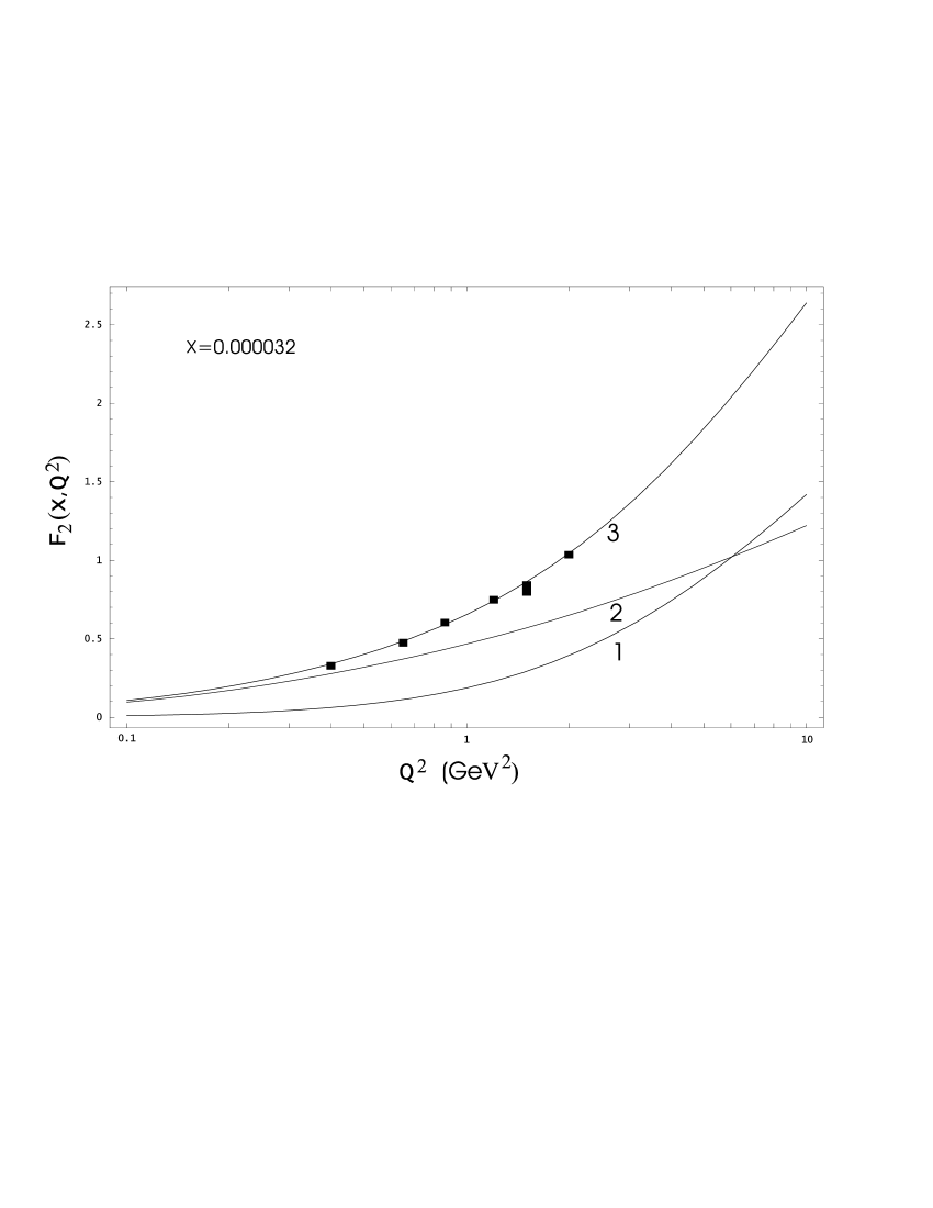
Figure 2: The proton structure function $F_{2}$, for the fixed value of $x_{Bj}$, as a function of $Q^{2}$. 1: hard component (the set of parameters, given by Eq.(4.10), is used); 2: GVDM part (formulae (B1) and (B2) are used); 3: summary curve. Experimental points are taken from ref.[24].

The values of parameters in the expression (3.1) for the cross section $\sigma(r_{\bot},s)$ must be determined from the comparison of our model predictions with experimental data for small $x_{Bj}$. The example of such a comparison for the particular value $x_{Bj}=0.000032$ is shown on fig.2. It is seen from this figure that our GVDM prediction for $F_{2}(x_{Bj},Q^{2})$ is clearly at variance with data even in the region of relatively low values of $Q^{2}$, if $x_{Bj}$ is small enough. At the same time, one can see that even at very small $x_{Bj}$ there is a $Q^{2}$-region, in which the hard component is negligibly small and GVDM works well.

The set of parameter values in Eq.(3.1) found from this comparison and used for numerical calculations is the following:

$$~{}~{}~{}a_{1}=0.99,~{}~{}~{}a_{2}=0.7GeV,~{}~{}~{}a_{3}=-6.23GeV^{2},$$

$$r_{\bot}^{0}=0.219GeV^{-1},~{}~{}~{}~{}\lambda_{H}=0.387.$$

This set differs from that obtaned in ref.[15] only by the smaller value of the parameter $r_{\bot}^{0}$.

5.Results of calculations

We performed calculations of the photonuclear cross section and energy loss coefficient for muons and tau-leptons.

As is mentioned in the Introduction, muons and taus of super high energies ($\gtrsim 10^{5}GeV$) are of natural origin: they appear as a result of interactions of superhigh energy cosmic rays in atmosphere (muons) and as a result of $\nu_{\mu}$( or $\nu_{e}$ )$\to\nu_{\tau}$ oscillations of extragalactic neutrinos on their way to the Earth with their subsequent interaction somewhere near the (underground) detector (taus). Therefore, we need, in practice, in the case of superhigh energies of leptons, the cross section of the inelastic lepton scattering on a nuclear target rather than on a nucleon one.

In the nonperturbative part of the cross section the nuclear shadowing effects are taken into account (formula (4.6)). As for the perturbative piece, the problem of the nuclear shadowing requires a special investigation which will be performed in a separate work. Qualitatively, the shadowing effects are small if the exponential term in the integral in the expression for the $(\stackrel{{\scriptstyle\,~{}-}}{{qq}})Z$ interaction cross section,

$$\sigma_{\stackrel{{\scriptstyle\,~{}-}}{{qq}}+Z}(r_{\bot},s)=2\int d^{2}b\{1-exp[-\sigma(r_{\bot},s)T(\stackrel{{\scriptstyle\to}}{{b}})/2]\},$$

is close to 1. In this formula $T(\stackrel{{\scriptstyle\to}}{{b}})$ is an optical thickness of the target nucleus at an impact parameter $\stackrel{{\scriptstyle\to}}{{b}}$,

$$T(\stackrel{{\scriptstyle\to}}{{b}})=\int\rho_{A}(b,z)dz.$$

The shadowing effects are small if

$$\sigma^{2}(r_{\bot},s)\frac{T^{2}(\stackrel{{\scriptstyle\to}}{{b}})}{8}<<\sigma(r_{\bot},s)\frac{T(\stackrel{{\scriptstyle\to}}{{b}})}{2},$$

or

$$\sigma_{max}(r_{\bot},s)<<\frac{4}{T(\stackrel{{\scriptstyle\to}}{{b}})}\lesssim\frac{4}{2R_{A}\rho_{A}}\sim\frac{8r^{2}_{0}}{A^{1/3}}.$$

Here, $\sigma_{max}$ is the maximum value of the $(\stackrel{{\scriptstyle\,~{}-}}{{qq}})p$ interaction cross section, $r_{0}\simeq 1.2$fm. If $A=22$ (it is the value which we use in all numerical calculations in the present paper), Eq.(5.4) gives the condition

$$\sigma_{max}(r_{\bot},s)<<40mb.$$

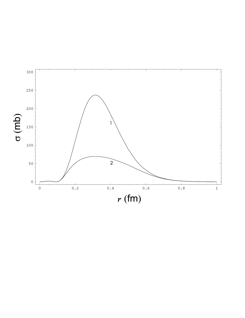
Figure 3: The total cross section of an interaction of the $\stackrel{{\scriptstyle\,~{}-}}{{qq}}$-pair of the transverse size $r_{\bot}$ with a target proton, $\sigma(r_{\bot},s)$. 1: Eq.(3.1); 2: the unitarized cross section (Eq.(3.6)). $s=10^{8}GeV^{2}$ in both cases.

The example of the calculation of $\sigma(r_{\bot},s)$ is shown on fig.3, and it is seen that the condition (5.5) is violated only at very high values of $s$, $s>10^{8}GeV^{2}$. It corresponds to typical lepton energies $E=\nu/v\sim s/(2M_{p}\cdot 0.1)\sim 10^{9}GeV$. Besides, the condition (5.5) is unnecessarily strong and can be weakened by taking into account that the nuclear shadowing effect in perturbative part of $\sigma^{A}_{T,L}$ strongly depends on $Q^{2}$ because, due to properties of Bessel functions in the expressions for photon wave functions (Eqs. 2.16), one has

$$\stackrel{{\scriptstyle-}}{{Q}}r_{\bot}\lesssim 1,$$

and, correspondingly,

$$r^{2}_{\bot char}\lesssim\frac{1}{Q^{2}},$$

where $r_{\bot char}$ is some characteristic value of a transverse size of the $\stackrel{{\scriptstyle\,~{}-}}{{qq}}$-pair in the nonperturbative interaction. The integral over $Q^{2}$ determining the photonuclear cross section $v\frac{d\sigma}{dv}$ is dominated by $Q^{2}$ values near $Q^{2}_{min}$ and, therefore, the role of $\stackrel{{\scriptstyle\,~{}-}}{{qq}}$-pairs with large $r_{\bot}$, for which the cross section $\sigma(r_{\bot},s)$ is relatively small, is, due to Eq.(5.7), sufficient.Accordingly, shadowing effects cannot be too large.

Note that the value of $r_{\bot}$ at which the cross section $\sigma(r_{\bot},s)$ has a maximum value does not coincide (even approximately) with a value of the parameter $r_{\bot}^{0}$ in the formula (3.1) (it is due to a large value of the parameter $a_{3}$, leading to a fast reveal of the $a_{3}r^{3}$-term). So, the typical pair’s transverse size corresponding to the perturbative interaction is determined, in the parameterization of ref.[15], by the combination of two parameters, $a_{3}$ and $r_{\bot}^{0}$.

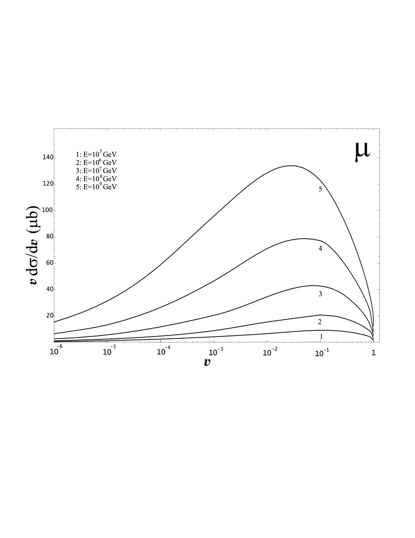
Figure 4: The perturbative part of the differential photonuclear ($\mu A$) cross section for $A=22$ (integrated over $Q^{2}$), as a function of $v$, the fraction of the muon energy transferred to hadrons, for several values of an initial energy of the muon. The expressions (4.4), (2.15), (2.16), (3.6), and the set of parameters (4.10) are used for the calculation.

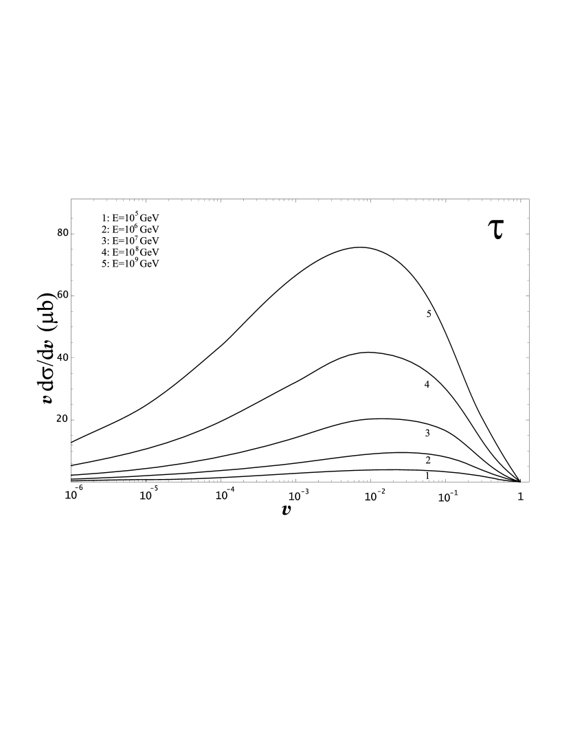
Figure 5: The same as fig.4, except the change $\mu\to\tau$.

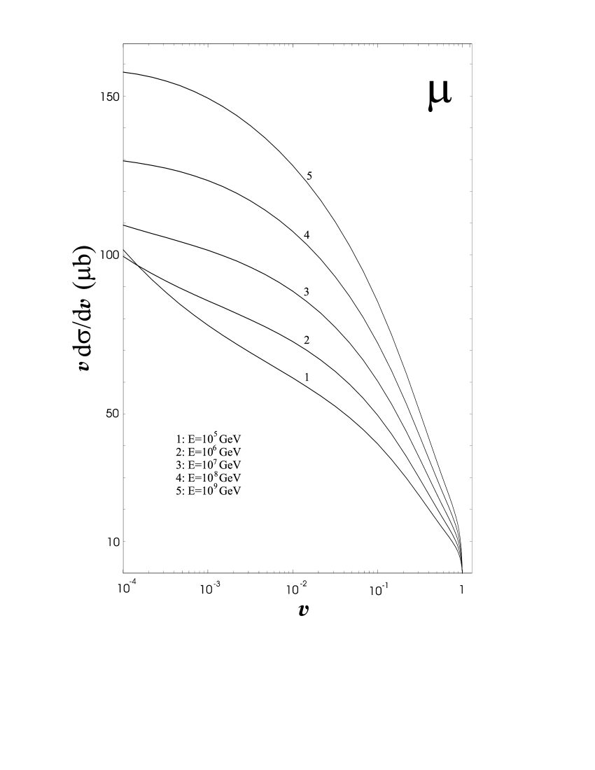
Figure 6: The nonperturbative part of the differential photonuclear ($\mu A$) cross section calculated using Eq.(4.6), for $A=22$.

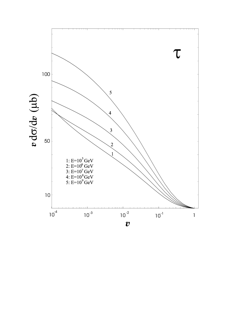
Figure 7: The same as fig.6, except the change $\mu\to\tau$.

The results of our calculation of the perturbative part of $v\frac{d\sigma}{dv}$ are shown on figs.4,5(for $\mu A$ and $\tau A$ interactions). These results can be used, together with the corresponding nonperturbative parts (given by Eq.(4.6)), for calculations of a $\mu$ and $\tau$ propagation through thick layers of matter and for calculations of detection probabilities of superhigh energy leptons passing through large underground telescopes. For completeness, we present on figs.6,7 also the nonperturbative parts of $v\frac{d\sigma}{dv}$. All calculations on figs.4-7 are done for standard rock, $A=22$.

For a rough estimate of the photonuclear range of leptons in matter it is useful to know the energy loss coefficients,

$$-\frac{1}{E}\frac{dE}{dx}=b(E,m_{l})=\frac{N_{A}}{A}\int v\frac{d\sigma}{dv}(E,v,m_{l}),$$

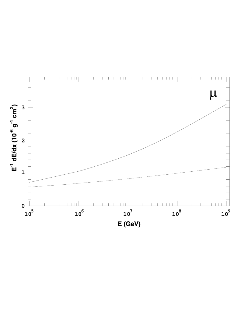
Figure 8: The energy loss coefficient for a muon, as a function of its energy, for standard rock($A=22$). The solid line is the total coefficient, the dashed line is the nonperturbative part calculated using BB formulae [5].

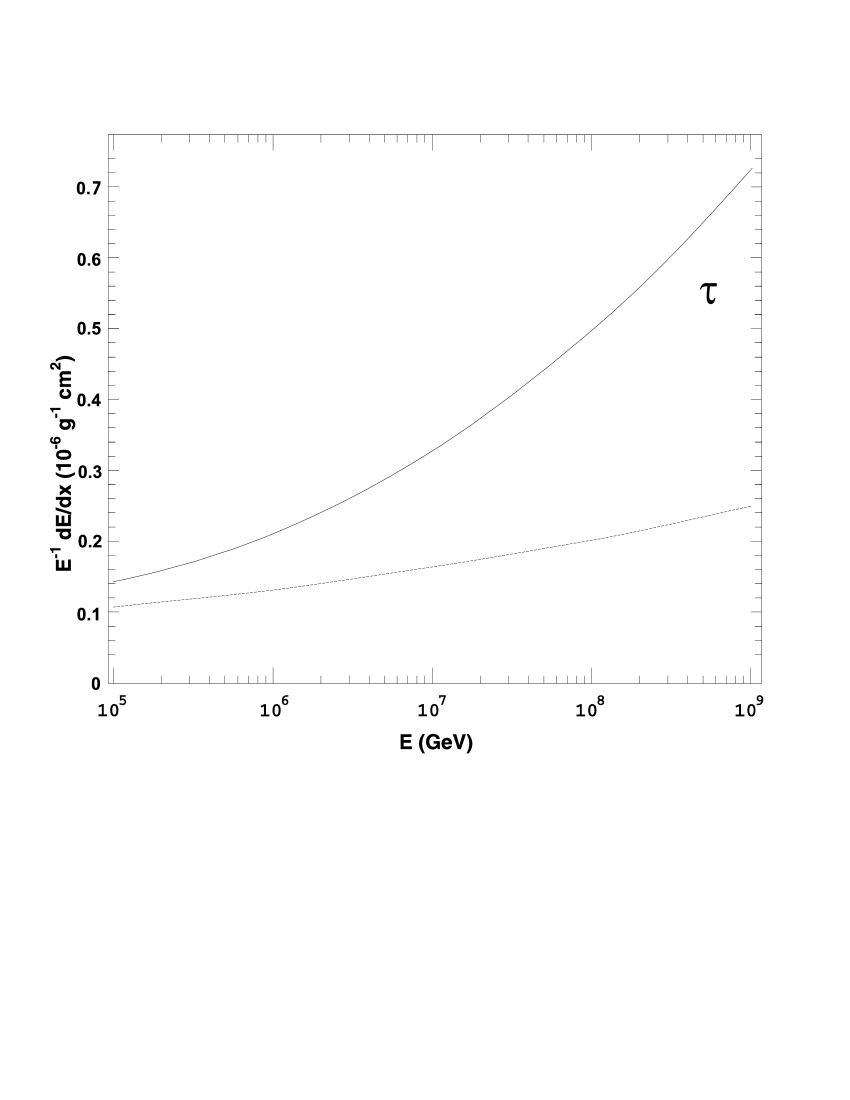
Figure 9: The same as fig.8, except the change $\mu\to\tau$.

(in a case of the perturbative part, if there is no shadowing, $v\frac{d\sigma}{dv}\sim A$ and we return to Eq.(4.8)). On figs.8,9 we show the results of calculations of such coefficients for standard rock. It is seen that at energies $E\sim 10^{8}-10^{9}GeV$ the contribution of the perturbative QCD part of the total photonuclear interaction in the lepton photonuclear energy losses is dominant ($\sim 70\%$).

The quantitatively similar results for the photonuclear energy loss coefficients $b(E,m_{l})$ were obtained in ref.[1], authors of which used for the description of the structure functions ALLM[25] parameterization (based on the Regge approach), and in ref.[26], for smaller energy interval ($E<10^{6}~{}GeV$) and only for muons (authors of [26] used for $\sigma_{T,L}$ the predictions of CKMT[27] model (also of Regge type)). Needless to say, that the theoretical approaches of refs.[25,27] are completely different from the one presented here.

Appendix A: The cut-off functions

In the case of transversely polarized virtual photons the criterion (2.14) and Eqs.(2.3) lead to the change (in the approximation $m_{f}=0$; $\Theta(x)$ is the step function )

$$\frac{3}{2}\int\limits^{1}_{0}dz[z^{2}+(1-z)^{2}]\longrightarrow\frac{3}{2}\int\limits^{1}_{0}dz[z^{2}+(1-z)^{2}\times$$

$$\times\Theta(\frac{k_{\bot 0}^{2}}{M^{2}(1+\frac{Q^{2}}{M^{2}})^{2}}-z(1-z))\Theta(\frac{k_{\bot 0}^{2}}{{M^{\prime}}^{2}(1+\frac{Q^{2}}{{M^{\prime}}^{2}})^{2}}-z(1-z))\equiv$$

$$\equiv\eta_{T}(M^{2},{M^{\prime}}^{2},k_{\bot 0}^{2}).$$

In diagonal approximation one obtains

$$\eta_{T}(M^{2},M^{2},k_{\bot 0}^{2})\equiv\eta_{T}(M^{2},k_{\bot 0}^{2})=3z_{0}-3z^{2}_{0}+2z^{3}_{0},$$

$$z_{0}=\frac{1}{2}-\sqrt{\frac{1}{4}-\frac{k_{\bot 0}^{2}}{M^{2}(1+\frac{Q^{2}}{M^{2}})^{2}}}.$$

If $M^{2}>>k_{\bot 0}^{2}$ one has

$$z_{0}\cong\frac{k_{\bot 0}^{2}}{M^{2}(1+\frac{Q^{2}}{M^{2}})^{2}},~{}~{}\eta_{T}(M^{2},k_{\bot 0}^{2})\cong 3\frac{k_{\bot 0}^{2}}{M^{2}(1+\frac{Q^{2}}{M^{2}})^{2}}.$$

Having in mind that nonperturbative $(\stackrel{{\scriptstyle\,~{}-}}{{qq}})p$ interaction amplitudes are essentially diagonal (it is known that, in the black disc limit, at least, the cross sections of nondiagonal diffractive processes should be small), we can approximate $\eta_{T}(M^{2},{M^{\prime}}^{2},k_{\bot 0}^{2})$ by the formula

$$\eta_{T}(M^{2},{M^{\prime}}^{2},k_{\bot 0}^{2})\cong\sqrt{\eta_{T}(M^{2},k_{\bot 0}^{2})\eta_{T}({M^{\prime}}^{2},k_{\bot 0}^{2})}.$$

In the case of longitudinally polarized photons the analogue of Eq.(A1) is

$$\frac{3}{2}\int\limits^{1}_{0}dz4z(1-z)\longrightarrow\frac{3}{2}\int\limits^{1}_{0}dz4z(1-z)\Theta(\frac{k_{\bot 0}^{2}}{M^{2}(1+\frac{Q^{2}}{M^{2}})^{2}}-z(1-z))\times$$

$$\times\Theta(\frac{k_{\bot 0}^{2}}{{M^{\prime}}^{2}(1+\frac{Q^{2}}{{M^{\prime}}^{2}})^{2}}-z(1-z))\equiv\eta_{L}(M^{2},{M^{\prime}}^{2},k_{\bot 0}^{2}),$$

and, in diagonal approximation ,

$$\eta_{L}(M^{2},M^{2},k_{\bot 0}^{2})\equiv\eta_{L}(M^{2},k_{\bot 0}^{2})=6z^{2}_{0}-4z^{3}_{0}.$$

Similarly with the previous case we approximate $\eta_{L}(M^{2},{M^{\prime}}^{2},k_{\bot 0}^{2})$ by the formula

$$\eta_{L}(M^{2},{M^{\prime}}^{2},k_{\bot 0}^{2})\cong\sqrt{\eta_{L}(M^{2},k_{\bot 0}^{2})\eta_{L}({M^{\prime}}^{2},k_{\bot 0}^{2})}.$$

1 Appendix B: Parameterization of structure functions in GVDM

In the GVDM version of ref.[5], the electromagnetic structure functions of a proton are well parameterized by the following expressions:

$$\sigma_{T}(Q^{2},\nu)=\sigma_{\gamma p}(\nu)\left\{0.75\frac{m^{4}_{1}}{(m^{2}_{1}+Q^{2})^{2}}+0.25\frac{m^{2}_{2}}{m^{2}_{2}+Q^{2}}\right\},$$

$$\sigma_{L}(Q^{2}.\nu)=\xi\sigma_{\gamma p}(\nu)\{0.75\frac{m^{2}_{1}Q^{2}}{(m^{2}_{1}+Q^{2})^{2}}+$$

$$+0.25[\frac{m^{2}_{2}}{Q^{2}}ln(1+\frac{Q^{2}}{m^{2}_{2}})-\frac{m^{2}_{2}}{m^{2}_{2}+Q^{2}}]\},$$

$$m^{2}_{1}=0.54~{}GeV^{2},~{}~{}m^{2}_{2}=1.8~{}GeV^{2},~{}~{}\xi=0.25.$$

In these formulae $\sigma_{\gamma p}(\nu)$ is the total photoproduction cross section for a real photon of energy $\nu$, which was parametrized by the equation [5]

$$\sigma_{\gamma p}(\nu)=114.3+1.647ln^{2}(0.0213\nu)~{}\mu b$$

($\nu$ is in units of $GeV$). The parameterization (B1,B2) works rather well in the small $Q^{2}-$region ($Q^{2}\lesssim 1~{}GeV^{2}$) and in the region of not very small $x_{Bj}$ ($10^{-3}<x_{Bj}<10^{-1}$), and does not contradict with the most recent H1 and ZEUS data.

The generalization of Eqs.(B1,B2) for nuclear targets is the following [5]: one must introduce the common factor $A$ and multiply the first term in figure brackets in right-hand-sides in Eqs.(B1,B2) by the shadowing function $G_{sh}(x)$ defined by the relation

$$G_{sh}(x)=\frac{3}{x^{3}}(\frac{x^{2}}{2}-1+e^{-x}(1+x)),$$

$$x\equiv 0.00282A^{1/3}\sigma_{\gamma p}(\nu).$$

As a result, one obtains

$$\sigma^{A}_{T}(Q^{2},\nu)=A\sigma_{\gamma p}(\nu)\{0.75\frac{m^{4}_{1}}{(m^{2}_{1}+Q^{2})^{2}}G_{sh}(x)+0.25\frac{m^{2}_{2}}{m^{2}_{2}+Q^{2}}\},$$

$$\sigma^{A}_{L}(Q^{2},\nu)=A\sigma_{\gamma p}(\nu)\xi\{0.75\frac{m^{2}_{1}Q^{2}}{(m^{2}_{1}+Q^{2})^{2}}G_{sh}(x)+$$

$$+0.25[\frac{m^{2}_{2}}{Q^{2}}ln(1+\frac{Q^{2}}{m^{2}_{2}})-\frac{m^{2}_{2}}{m^{2}_{2}+Q^{2}}]\}.$$

References

- [1] S. I. Dutta, M. H. Reno, I. Sarcevic, and D. Seckel, Phys. Rev. D63, 094020 (2001).
- [2] E.V.Bugaev, B.V.Mangazeev, Yu.V.Shlepin, hep-ph/9912384.
- [3] E. Gotsman, E. M. Levin, and U. Maor, Eur. Phys. J. C5, 303 (1998).
- [4] A. D. Martin, M. G. Ryskin, and A. M. Stasto, Eur. Phys. J. C7, 643 (1999).
- [5] L. B. Bezrukov and E. V. Bugaev, Sov. J. Nucl. Phys. 33, 635 (1981).
- [6] N. N. Nikolaev and B. G. Zakharov, Z. Phys. C49, 607 (1991); Z. Phys. C53, 331 (1992); Z. Phys. C64, 631 (1994).
- [7] F. E. Low, Phys. Rev. D12, 163 (1975).
- [8] S. Nussinov, Phys. Rev. Lett. 34, 1286 (1975).
- [9] J. Gunion and D. Soper, Phys. Rev. D15, 2617 (1977).
- [10] E. M. Levin and M. G. Ryskin, Yad. Fiz. 34, 1114 (1981); Sov. J. Nucl. Phys. 45, 150 (1987).
- [11] A. H. Mueller, Nucl. Phys. B335, 115 (1990); Nucl. Phys. B415, 373 (1994).
- [12] L. Frankfurt, G. A. Miller, and M. I. Strikman, Phys. Lett. B304, 1 (1993).
- [13] L. Frankfurt and M. I. Strikman, Nucl. Phys. B316, 340 (1989).
- [14] J. D. Bjorken, Proc. of the Int. Symp. on Electron and Photon Interactions at High Energies, Cornell University (1971).
- [15] J. R. Forshaw, G. Kerley, and G. Shaw, Phys. Rev. D60, 074012 (1999).
- [16] V. N. Gribov, Sov. Phys. JETP, 30, 709 (1970).
- [17] J. J. Sakurai and D. Schildknecht, Phys. Lett. 40B, 121 (1972).
- [18] J. J. Sakurai, Phys. Rev. Lett. 22, 981 (1969).
- [19] T. H. Bauer, R. D. Spital, D. K. Yennie and F. M. Pipkin, Rev. Mod. Phys. 50, 261 (1978).
- [20] A. L. Ayala, M. B. Gay Ducati, and E. M. Levin, Phys. Lett. B388, 188 (1996).
- [21] H. Fraas, B. J. Read, and D. Schildknecht, Nucl. Phys. B86, 346 (1975).
- [22] P. Ditsas and G. Shaw, Nucl. Phys. B113, 246 (1976).
- [23] L. B. Bezrukov and E. V. Bugaev, Sov. J. Nucl. Phys. 32, 847 (1980).
- [24] Particle Data Group, Eur. Phys. J. C15, 220 (2000).
- [25] H. Abramowicz et al, Phys. Lett. B269, 465 (1991).
- [26] A. V. Butkevich and S. P. Mikheyev, hep-ph/0109060.
- [27] A. Capella et al, Phys. Lett. B337, 358 (1994).