A study of semi-inclusive charmless $B\to\pi X$ decays

Abstract

We study semi-inclusive charmless decays $B\to\pi X$ in detail, such as $\overline{B}^{0}\to\pi^{\pm(0)}X$, $B^{0}\to\pi^{\pm(0)}X$, $B^{\pm}\to\pi^{\pm(0)}X$, where $X$ does not contain a charm (anti)quark. We find that the process $\overline{B}^{0}\to\pi^{-}X$ ($B^{0}\to\pi^{+}X$) can be particularly useful for determination of the CKM matrix element $|V_{ub}|$. We calculate and present the branching ratio (BR) of $\overline{B}^{0}\to\pi^{-}X$ as a function of $|V_{ub}|$, with an estimate of possible uncertainties. It is expected that the BR is an order of $10^{-4}$. Our estimation indicates that one can phenomenologically determine $|V_{ub}|$ with reasonable accuracy by measuring the BR of $\overline{B}^{0}\to\pi^{-}X$ ($B^{0}\to\pi^{+}X$).

I Introduction

The source of CP violation in the Standard Model (SM) with three generations is a phase in the Cabibbo-Kobayashi-Maskawa (CKM) matrix [1]. A precise measurement of the CKM matrix elements is one of the key issues in the study of $B-$mesons and $B-$factory experiments. In particular, the accurate determination of $V_{ub}$ is one of the most challenging problems in $B$ physics. Its non-vanishing value is a necessary condition for CP violation to occur in the SM and its accurate value can put strong constraints even on the unitarity triangle: for instance, on the magnitude of the CP violating phase $\beta(\equiv\phi_{1})$.

Theoretical and experimental studies for probing $V_{ub}$ have been mostly focused on the semileptonic $B-$meson decays. The present best experimental data for $V_{ub}$ come from measurements of the exclusive decay $B\to\rho l\bar{\nu}$ and the inclusive decay $B\to X_{u}l\bar{\nu}$, but these measurements suffer from large uncertainties due to model-dependence and other theoretical errors. For example, the CLEO result obtained using the exclusive semileptonic decay $B\to\rho l\bar{\nu}$ [2] :

$$|V_{ub}|=(3.25\pm 0.14(\rm stat.)^{+0.21}_{-0.29}(\rm syst.)\pm 0.55(\rm model))\times 10^{-3}~{}.$$ (1)

The OPAL data obtained using the inclusive decay $B\to X_{u}l\bar{\nu}$ [3] :

$$|V_{ub}|=(4.00\pm 0.65(\rm stat.)^{+0.67}_{-0.76}(\rm syst.)\pm 0.19(\rm HQE))\times 10^{-3}~{}.$$ (2)

The method using the exclusive semileptonic decays involves hadronic form factors, such as $F^{B\to\pi}$ or $A^{B\to\rho}$, whose values are heavily model-dependent and cause large uncertainties. The difficulty of using the inclusive charmless decay $B\to X_{u}l\bar{\nu}$ is in discriminating this process from the dominant background $B\to X_{c}l\nu$ decay [4], whose branching ratio is more than 50 times larger than that of $B\to X_{u}l\bar{\nu}$.

Although traditional difficulties with the understanding of non-leptonic $B$ decays have prevented their use in determination of the CKM matrix elements, the possibility of measuring $|V_{ub}|$ via non-leptonic decays of $B-$mesons to exclusive or inclusive final states has been also theoretically explored [5, 6, 7, 8].

In this work we study semi-inclusive charmless decays $B\to\pi X$ and investigate the possibility of extracting $|V_{ub}|$ from these processes. Compared to the exclusive decays, these semi-inclusive decays are generally expected to have less hadronic uncertainties and larger branching ratios. There are several possible processes in $B\to\pi X$ type decays, such as $\overline{B}^{0}\to\pi^{\pm(0)}X$, $B^{0}\to\pi^{\pm(0)}X$, $B^{\pm}\to\pi^{\pm(0)}X$, where $X$ does not contain a charm (anti)quark. The class of nonleptonic two-body decay modes and their advantages within general arguments were previously discussed in Ref. [9], and semi-inclusive two-body decays within the QCD factorization were also studied in Ref. [10].

In Sec. II we first classify all those $B\to\pi X$ processes, and we identify a certain mode, $\overline{B}^{0}\to\pi^{-}X$, whose analysis is theoretically clean and which can be used for determining $|V_{ub}|$. Then, in Sec. III we study the mode $\overline{B}^{0}\to\pi^{-}X$ in detail and propose a method to extract $|V_{ub}|$. That is, we calculate the branching ratio (BR) of this mode using the full effective Hamiltonian in the framework of the generalized factorization, and present the result as a function of $|V_{ub}|$ with an estimation of possible uncertainties. We also consider the $B^{0}-\overline{B}^{0}$ mixing effect through $\overline{B}^{0}\to B^{0}\to\pi^{-}X$. The conclusions are in Sec. IV.

II Classification of Semi-inclusive charmless $B\to\pi X$ decays

Among the semi-inclusive charmless $B\to\pi X$ decays, let us first consider the mode $\overline{B}^{0}\to\pi^{-}X$. Contributions for the decay amplitude of this mode arise from the color-favored tree ($b\to u\bar{u}d$) diagram and the $b\to d$ penguin diagram (see Fig. 1), and the tree diagram contribution dominates.

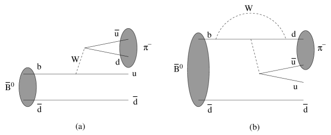
FIG. 1.: Feynman diagrams of $\overline{B}^{0}\to\pi^{-}X$ decay: (a) the color-favored tree diagram, and (b) the $b\to d$ penguin diagram.

The charged pion $\pi^{-}$ in the final state can be produced via $W-$boson emission at tree level and is expected to be energetic ($E_{\pi^{-}}\sim m_{B}/2$). The decay amplitude can be approximated as

$$A(\overline{B}^{0}\to\pi^{-}X)\simeq A(b\to\pi^{-}u)\cdot h(u\bar{d}\to X(u\bar{d}))\approx A(b\to\pi^{-}u)~{},$$ (3)

where $h$ denotes a hadronization function describing the combination of the $u\bar{d}$ pair to make the final state $X$. To obtain the decay rate, $X(u\bar{d})$ should be summed over all the possible states, such as $\pi^{+}\pi^{0}$, $\pi^{+}\pi^{+}\pi^{-}$ etc, so this process is effectively a two-body decay process of $b\to\pi^{-}u$ in the parton model approximation. Thus, in this specific mode, no hadronic form factors (except the pion decay constant $f_{\pi}$) are involved, and as a result the model-dependence does not appear to be severe. We note that the energetic charged pion $\pi^{-}$ in the final state can be a characteristic signal for this mode. We will show in Fig. 3 the decay distribution, $d\Gamma\over dE_{\pi}$, for $\overline{B}^{0}\to\pi^{-}X$ as a function of the charged pion energy $E_{\pi}$. (For a detailed explanation, see Sec. III.) Like a two-body decay, a peak appears around $E_{\pi^{-}}=m_{B}/2$.

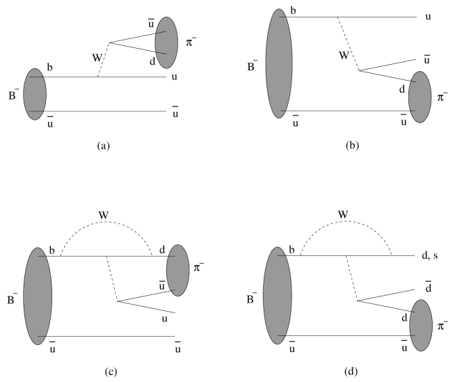
FIG. 2.: Feynman diagrams of $B^{-}\to\pi^{-}X$ decay: (a) the color-favored tree diagram, (b) the color-suppressed tree diagram, (c) the $b\to d$ penguin diagram, and (d) the $b\to d$ and $b\to s$ penguin diagram.

Now let us consider the mode $B^{-}\to\pi^{-}X$. As shown in Fig. 2, various contributions are responsible for this process: the color-favored tree diagram, the color-suppressed tree diagram, the $b\to d$ and $b\to s$ penguin diagrams. The color-favored tree contribution (Fig. 2(a)) and $b\to d$ penguin contributions (Fig. 2(c)) are similar to those in $\overline{B}^{0}\to\pi^{-}X$, which are effectively two-body type ($b\to\pi^{-}u$) processes. However, the color-suppressed tree (Fig. 2(b)) and other penguins (Fig. 2(d)) differ from those in $\overline{B}^{0}\to\pi^{-}X$. In fact, these two diagrams correspond to effectively a three-body decay process of $B^{-}\to\pi^{-}u\bar{u}$ (or $\pi^{-}d\bar{d}$) in the parton model approximation, with the decay amplitude

$$A(B^{-}\to\pi^{-}X)\simeq A(B^{-}\to\pi^{-}u\bar{u})\cdot h(u\bar{u}\to X(u\bar{u}))\approx A(B^{-}\to\pi^{-}u\bar{u})~{}.$$ (4)

In Figs. 2(b) and 2(d), the charged pion $\pi^{-}$ in the final state contains the spectator antiquark $\bar{u}$. So the analysis involves the hadronic form factor for the $B\to\pi$ transition which is highly model-dependent. Furthermore, the $b\to s$ penguin contribution (Fig. 2(d)) is not suppressed compared to the tree contributions, but dominant in this mode. The decay distribution, $d\Gamma\over dE_{\pi}$, for $B^{-}\to\pi^{-}X$ will be shown in Fig. 4, as a function of the charged pion energy $E_{\pi}$. The three-body type contribution from the $b\to s$ penguin is the dominant one. Therefore, compared to the case of $\overline{B}^{0}\to\pi^{-}X$, the analysis of this mode is much more complicated and involves larger uncertainties.

Other modes of the type $B\to\pi X$ can be similarly classified. For instance, in the mode $B^{0}\to\pi^{-}X$, the color-favored tree ($\bar{b}\to\bar{u}u\bar{d}$ and $\bar{b}\to\bar{u}u\bar{s}$) diagrams and the $b\to d$ and $b\to s$ penguin diagrams are responsible for the decay process. In this case, the charged pion $\pi^{-}$ contains the spectator quark $d$ so that the process is effectively a three-body decay $B^{0}\to\pi^{-}u\bar{d}~{}(\bar{s})$ and the hadronic form factor for the $B\to\pi$ transition is involved. Other processes are basically a combination of the two-body decay process ($b\to\pi q$) and the three-body decay process ($B^{-}\to\pi^{-}q\bar{q}^{\prime}$).

III Analysis of $\overline{B}^{0}\to\pi^{-}X$ decay

In the previous section, we have seen that the process $\overline{B}^{0}\to\pi^{-}X$ is particularly interesting, because it is effectively the two-body decay process $b\to\pi^{-}u$ in the parton model approximation, and no uncertainty from hadronic form factors is involved. Thus, its theoretical analysis is expected to be quite clean.

The relevant $\Delta B=1$ effective Hamiltonian for hadronic $B$ decays can be written as

$$H_{eff}^{q} = {G_{F}\over\sqrt{2}}\left[V_{ub}V^{*}_{uq}(c_{1}O^{q}_{1u}+c_{2}O^{q}_{2u})+V_{cb}V^{*}_{cq}(c_{1}O^{q}_{1c}+c_{2}O^{q}_{2c})\right.$$ (5)

$$- \left.\sum_{i=3}^{10}\left(V_{ub}V^{*}_{uq}c_{i}^{u}+V_{cb}V^{*}_{cq}c_{i}^{c}+V_{tb}V^{*}_{tq}c_{i}^{t}\right)O_{i}^{q}\right]$$ (6)

$$+ H.C.~{},$$ (7)

where $O^{q}_{i}$’s are defined as

$$O^{q}_{1f} = \bar{q}\gamma_{\mu}Lf\bar{f}\gamma^{\mu}Lb,\ \ O^{q}_{2f}=\bar{q}_{\alpha}\gamma_{\mu}Lf_{\beta}\bar{f}_{\beta}\gamma^{\mu}Lb_{\alpha}~{},$$ (8)

$$O^{q}_{3(5)} = \bar{q}\gamma_{\mu}Lb\sum_{q^{\prime}}\bar{q}^{\prime}\gamma^{\mu}L(R)q^{\prime},\ \ O^{q}_{4(6)}=\bar{q}_{\alpha}\gamma_{\mu}Lb_{\beta}\sum_{q^{\prime}}\bar{q}^{\prime}_{\beta}\gamma^{\mu}L(R)q^{\prime}_{\alpha}~{},$$ (9)

$$O^{q}_{7(9)} = {3\over 2}\bar{q}\gamma_{\mu}Lb\sum_{q^{\prime}}e_{q^{\prime}}\bar{q}^{\prime}\gamma^{\mu}R(L)q^{\prime},\ \ O^{q}_{8(10)}={3\over 2}\bar{q}_{\alpha}\gamma_{\mu}Lb_{\beta}\sum_{q^{\prime}}e_{q^{\prime}}\bar{q}^{\prime}_{\beta}\gamma^{\mu}R(L)q^{\prime}_{\alpha}~{},$$ (10)

where $L(R)=(1\mp\gamma_{5})$, $f$ can be $u$ or $c$ quark, $q$ can be $d$ or $s$ quark, and $q^{\prime}$ is summed over $u$, $d$, $s$, and $c$ quarks. $\alpha$ and $\beta$ are the color indices. $c_{i}$’s are the Wilson coefficients (WC’s), and we use the effective WC’s for the process $b\to d\bar{q}q^{\prime}$ from Ref.[11]. The regularization scale is taken to be $\mu=m_{b}$. The operators $O_{1}$, $O_{2}$ are the tree level and QCD corrected operators, $O_{3-6}$ are the gluon induced strong penguin operators, and finally $O_{7-10}$ are the electroweak penguin operators due to $\gamma$ and $Z$ exchange, and the box diagrams at loop level.

Now we calculate the decay amplitude for the semi-inclusive decay $\overline{B}^{0}\to\pi^{-}X$, where $X$ can contain an up quark and a down antiquark. In the generalized factorization approximation, the decay amplitude is given by

$${\cal M} = \langle\pi^{-}X|H_{eff}|\overline{B}^{0}\rangle~{},$$ (11)

$$= i{G_{F}\over\sqrt{2}}f_{\pi}\langle X|\bar{u}\left[r(1+\gamma^{5})+l(1-\gamma^{5})\right]b|\overline{B}^{0}\rangle~{},$$ (12)

where we have defined the followings:

$$r = m_{b}w_{1}~{},$$ (13)

$$l = -m_{u}w_{1}-{m_{\pi}^{2}\over m_{d}+m_{u}}w_{2}~{},$$ (14)

$$w_{1} = V_{ub}V^{*}_{ud}\left({c_{1}\over N_{c}}+c_{2}\right)+{A_{3}\over N_{c}}+A_{4}+{A_{9}\over N_{c}}+A_{10}~{},$$ (15)

$$w_{2} = -2\left({A_{5}\over N_{c}}+A_{6}+{A_{7}\over N_{c}}+A_{8}\right)~{}.$$ (16)

Here $N_{c}$ denotes the effective number of color and

$$A_{i} = -\sum_{q=u,c,t}V_{qb}V^{*}_{qd}c^{q}_{i}\ .$$ (17)

We have used the relations

$$\langle\pi^{-}|\bar{d}\gamma^{\mu}\gamma^{5}u|0\rangle = -if_{\pi}p^{\mu}_{\pi}~{},$$ (18)

$$\langle\pi^{-}|\bar{d}\gamma^{5}u|0\rangle = -i{f_{\pi}m^{2}_{\pi}\over m_{d}+m_{u}}~{},$$ (19)

where $f_{\pi}$ and $p^{\mu}_{\pi}$ are the decay constant and the momentum of pion, respectively, and $m_{\pi}~{}(m_{i})$ is the mass of pion ($i$ quark). In Eq. (19) the free quark equation of motion has been used.

Then,

$$|{\cal M}|^{2} = {G_{F}^{2}\over 2}f_{\pi}^{2}\sum_{X}\left|\langle X|\bar{u}\left[r(1+\gamma^{5})+l(1-\gamma^{5})\right]b|\overline{B}^{0}\rangle\right|^{2}(2\pi)^{4}\delta^{4}(p_{B}-p_{\pi}-p_{X})$$ (20)

$$= {G_{F}^{2}\over 2}f_{\pi}^{2}\sum_{X}\langle\overline{B}^{0}|J|X\rangle\langle X|J^{\dagger}|\overline{B}^{0}\rangle(2\pi)^{4}\delta^{4}(p_{B}-p_{\pi}-p_{X})~{},$$ (21)

where

$$J^{\dagger}=\bar{u}\left[r(1+\gamma^{5})+l(1-\gamma^{5})\right]b~{}.$$ (22)

In the parton model approximation we take the leading order term in the product of the above matrix elements, which corresponds to interpretation of the above process as $b(p_{b})\rightarrow\pi^{-}(p_{\pi})+u(p_{u})$ [12]. Then, $|{\cal M}|^{2}$ can be expressed as

$$|{\cal M}|^{2} = 2G_{F}^{2}f_{\pi}^{2}\left[(|r|^{2}+|l|^{2})(p_{u}\cdot p_{b})+2Re(rl^{*})m_{u}m_{b}\right]$$ (23)

$$= |V_{ub}|^{2}{\cal M}_{2}+|V_{ub}|{\cal M}_{1}+{\cal M}_{0}~{},$$ (24)

where

$${\cal M}_{2} = 2G_{F}^{2}f_{\pi}^{2}|V_{ud}^{*}|^{2}\{|c^{ut}|^{2}{\cal X}+4|\tilde{c}^{ut}|^{2}{\cal Y}+2Re[(c^{ut})(\tilde{c}^{ut})^{*}]{\cal Z}\}~{},$$ (25)

$${\cal M}_{1} = 2G_{F}^{2}f_{\pi}^{2}|V_{ud}V_{cb}V_{cd}^{*}|\{2Re[e^{i\gamma}(c^{ct})(c^{ut})^{*}]{\cal X}+8Re[e^{i\gamma}(\tilde{c}^{ct})(\tilde{c}^{ut})^{*}]{\cal Y}$$ (26)

$$+ 2Re[e^{i\gamma}(c^{ct})(\tilde{c}^{ut})^{*}+e^{-i\gamma}(c^{ut})(\tilde{c}^{ct})^{*}]{\cal Z}\}~{},$$ (27)

$${\cal M}_{0} = 2G_{F}^{2}f_{\pi}^{2}|V_{cb}V_{cd}^{*}|^{2}\{|c^{ct}|^{2}{\cal X}+4|\tilde{c}^{ct}|^{2}{\cal Y}+2Re[(c^{ct})(\tilde{c}^{ct})^{*}]{\cal Z}\}~{},$$ (28)

and

$${\cal X} = (m_{b}^{2}+m_{u}^{2})(p_{b}\cdot p_{u})-2m_{b}^{2}m_{u}^{2}~{},$$ (29)

$${\cal Y} = {m_{\pi}^{4}\over(m_{d}+m_{u})^{2}}(p_{b}\cdot p_{u})~{},$$ (30)

$${\cal Z} = {2m_{u}m_{\pi}^{2}\over m_{d}+m_{u}}(p_{b}\cdot p_{u}-m_{b}^{2})~{},$$ (31)

$$c^{ut} = \left({c_{1}\over N_{c}}+c_{2}\right)-{1\over N_{c}}(c_{3}^{u}-c_{3}^{t})-(c_{4}^{u}-c_{4}^{t})-{1\over N_{c}}(c_{9}^{u}-c_{9}^{t})-(c_{10}^{u}-c_{10}^{t})~{},$$ (32)

$$c^{ct} = -{1\over N_{c}}(c_{3}^{c}-c_{3}^{t})-(c_{4}^{c}-c_{4}^{t})-{1\over N_{c}}(c_{9}^{c}-c_{9}^{t})-(c_{10}^{c}-c_{10}^{t})~{},$$ (33)

$$\tilde{c}^{qt} = {1\over N_{c}}(c_{5}^{q}-c_{5}^{t})+(c_{6}^{q}-c_{6}^{t})+{1\over N_{c}}(c_{7}^{q}-c_{7}^{t})+(c_{8}^{q}-c_{8}^{t})\ \ \ (q=u,c)~{}.$$ (34)

Here we have used the usual definition of the phase angle,

$$\gamma(\equiv\phi_{3})=Arg[-(V_{ud}V^{*}_{ub})/(V_{cd}V^{*}_{cb})]~{}.$$ (35)

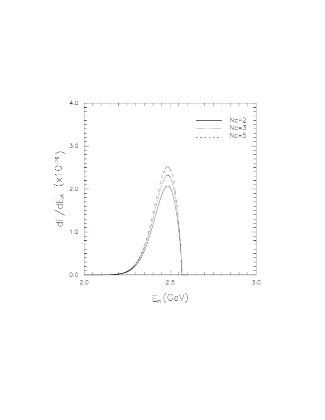
FIG. 3.: $d\Gamma\over dE_{\pi}$ (in units of $10^{-16}$) versus $E_{\pi}$ for $\overline{B}^{0}\to\pi^{-}X$ decay. The solid, dotted, and dashed lines correspond to $N_{c}=2,~{}3,~{}5$, respectively.

FIG. 4.: $d\Gamma\over dE_{\pi}$ (in units of $10^{-16}$) versus $E_{\pi}$ for $B^{-}\to\pi^{-}X$ decay. The solid, dotted, and dashed lines correspond to $N_{c}=2,~{}3,~{}5$, respectively. Here, ‘2body_u’ stands for the two-body type ($b\to\pi^{-}u)$ processes (see Fig. 2(a,c)), and ‘3body_ds’ stands for the three-body type processes from the color-suppressed tree and the $b\to d$ and $b\to s$ penguins (Fig. 2(b,d)), while ‘3body_d’ stands for the three-body type process from the $b\to d$ penguin only (Fig. 2(d)).

We first calculate the decay distribution in the $b$ quark rest frame and boost it to the $B-$meson rest frame. In the $b$ quark rest frame, the decay distribution is given by

$$\left.{d\Gamma\over dE_{\pi}}\right|_{b}={1\over 16\pi}|{\cal M}|^{2}{p_{\pi}\over m_{b}E_{u}}\delta(m_{b}-E_{\pi}-E_{u})~{}.$$ (36)

In the $B-$meson rest frame, the $b$ quark is in motion and has the energy $E_{b}$ satisfying the relation: $E_{b}=m_{B}-E_{u}~{}$, where $E_{i}=\sqrt{p^{2}+m^{2}_{i}}$. $E_{i}$ and $m_{i}$ denote the energy and the mass of $i$ quark inside the $B-$meson, respectively. The 3-momentum $p$ is defined by $p=|\vec{p}_{b}|=|\vec{p}_{u}|$. Thus, the $b$ quark mass is now a function of $p$ given by

$$m_{b}^{2}(p)=m_{B}^{2}+m_{u}^{2}-2m_{B}\sqrt{p^{2}+m_{u}^{2}}~{}.$$ (37)

The decay distribution in the $B$ rest frame can be calculated by

$${d\Gamma\over dE_{\pi}}=\int^{p_{max}}_{0}dp\;p^{2}\phi(p)\left.{d\Gamma\over dE_{\pi}}\right|_{b}~{},$$ (38)

where $p_{max}=(m_{B}^{2}-m_{u}^{2})/(2m_{B})$. We have used the ACCMM model [13] using the $B-$meson wave function:

$$\phi(p)={4\over\sqrt{\pi p_{{}_{F}}^{3}}}e^{-p^{2}/p_{{}_{F}}^{2}}~{},$$ (39)

with the normalization $\int_{0}^{\infty}p^{2}\phi(p)dp=1$.

TABLE I.: The branching ratio (BR) of $\overline{B}^{0}\to\pi^{-}X$ for fixed $\gamma=65^{0}$. Here ${\cal B}$ denotes the BR calculated for $|V_{ub}|=0.004$.

$N_{c}$	${\cal B}\times 10^{4}$	${\cal B}_{2}\times 10^{4}$	${\cal B}_{1}\times 10^{4}$	${\cal B}_{0}\times 10^{4}$
2	1.05	0.89	0.14	0.016
3	1.17	0.98	0.17	0.019
4	1.24	1.03	0.19	0.020
5	1.27	1.06	0.19	0.021

The Fermi momentum $p_{{}_{F}}=0.3{\rm GeV}$ has been used. In Figs. 3 and 4 we show the decay distributions for $\overline{B}^{0}\to\pi^{-}X$ and $B^{-}\to\pi^{-}X$ as a function of the charged pion energy $E_{\pi}$. For $\overline{B}^{0}\to\pi^{-}X$ decay, the distribution has a peak at $E_{\pi}\simeq m_{B}/2$. This is a characteristic of a two-body decay. Because the $b$ quark inside the $\overline{B}^{0}$ is in motion, the distribution has some width shown in Fig. 3. For $B^{-}\to\pi^{-}X$, the decay distribution is a mixture of three-body type decay distributions and a two-body type decay distribution. Figure 4 shows that the dominant contribution arises from a three-body type decay (the $b\to s$ penguin process), as explained in Sec. II.

The BR of $\overline{B}^{0}\to\pi^{-}X$ can be expressed as a polynomial of $|V_{ub}|$:

$${\cal B}(\overline{B}^{0}\to\pi^{-}X)=\left|{V_{ub}\over 0.004}\right|^{2}\cdot{\cal B}_{2}+\left|{V_{ub}\over 0.004}\right|\cdot{\cal B}_{1}+{\cal B}_{0}~{},$$ (40)

where for convenience we have scaled $|V_{ub}|$ by the factor 0.004 (the central value of the OPAL data). Tables I and II show the BR of $\overline{B}^{0}\to\pi^{-}X$ for fixed $\gamma(\equiv\phi_{3})=65^{\circ}$ and $N_{c}=3$, respectively, with a fixed input value of $|V_{ub}|=0.004$. We note that the term ${\cal B}_{2}$ is the dominant contribution ($\sim 10^{-4}$) to ${\cal B}$, while the contribution from the term ${\cal B}_{0}$ is very small ($\sim 10^{-6}$). This is due to the fact (see Fig. 1) that ${\cal B}_{2}$ corresponds to mostly the tree contribution ($b\to u\bar{u}d$), while ${\cal B}_{0}$ corresponds to the pure $b\to d$ penguin contribution which is very small compared to the tree contribution, and ${\cal B}_{1}$ corresponds to the interference between them. We see that the BR of $\overline{B}^{0}\to\pi^{-}X$ is about $10^{-4}$ for different values of $\gamma(\equiv\phi_{3})$ and $N_{c}$.

FIG. 5.: The branching ratio (in units of $10^{-4}$) versus the effective number of color, $N_{c}$, for $\overline{B}^{0}\to\pi^{-}X$ decay. $B_{tot}(\equiv{\cal B})$ has been calculated using $|V_{ub}|=0.004$ and is denoted by the bold solid line. The solid, dotted, and dashed lines correspond to $\gamma=65^{\circ},~{}85^{\circ},~{}110^{\circ}$, respectively. For light quark masses, $m_{u}=5$ MeV and $m_{d}=7$ MeV have been used.

TABLE II.: The branching ratio of $\overline{B}^{0}\to\pi^{-}X$ for fixed $N_{c}=3$. Here ${\cal B}$ denotes the BR calculated for $|V_{ub}|=0.004$.

$\gamma$	${\cal B}\times 10^{4}$	${\cal B}_{2}\times 10^{4}$	${\cal B}_{1}\times 10^{4}$	${\cal B}_{0}\times 10^{4}$
60	1.18	0.98	0.18	0.019
70	1.16	0.98	0.16	0.019
80	1.14	0.98	0.14	0.019
90	1.11	0.98	0.11	0.019
100	1.07	0.98	0.072	0.019
110	1.04	0.98	0.037	0.019

FIG. 6.: The branching ratio (in units of $10^{-4}$) versus the CP phase, $\gamma$, for $\overline{B}^{0}\to\pi^{-}X$ decay. $B_{tot}(\equiv{\cal B})$ has been calculated using $|V_{ub}|=0.004$ and is denoted by the bold solid line. The solid, dotted, and dashed lines correspond to $N_{c}=2,~{}5,~{}10$, respectively. $m_{u}=5$ MeV and $m_{d}=7$ MeV have been used.

FIG. 7.: The branching ratio (in units of $10^{-4}$) versus $|V_{ub}|$ for $\overline{B}^{0}\to\pi^{-}X$ decay. The solid and the dotted lines correspond to the smallest and the largest value of ${\cal B}$ in the given parameter space, respectively. For light quark masses, $m_{u}=(1.5-5)$ MeV and $m_{d}=(3-9)$ MeV have been used.

In Fig. 5, we present the BR of $\overline{B}^{0}\to\pi^{-}X$ as a function of $N_{c}$ for three different values of $\gamma(\equiv\phi_{3})=65^{\circ},~{}85^{\circ},~{}110^{\circ}$. As one can see from Eqs. (24, 28, 40) and from Table 2 and Fig. 6, ${\cal B}_{2}$ and ${\cal B}_{0}$ are independent of $\gamma(\equiv\phi_{3})$, and only ${\cal B}_{1}$ depends on $\gamma(\equiv\phi_{3})$. Three different lines for ${\cal B}_{1}$ correspond to the relevant values of $\gamma(\equiv\phi_{3})$, respectively. It is clearly shown that ${\cal B}_{2}$ is dominant. A representative value of ${\cal B}$ for $|V_{ub}|=0.004$ and $\gamma(\equiv\phi_{3})=85^{\circ}$ is shown as the bold solid line in the figure. The value of ${\cal B}$ does not vary much as $N_{c}$ varies.

Similarly, Figure 6 shows the BR of $\overline{B}^{0}\to\pi^{-}X$ as a function of $\gamma(\equiv\phi_{3})$ for three different values of $N_{c}=2,~{}5,~{}10$. The solid line corresponds to the case $N_{c}=2$, and the dotted line and the dashed line are for $N_{c}=5$ and $N_{c}=10$, respectively. The ${\cal B}_{2}$, ${\cal B}_{1}$ and ${\cal B}_{0}$ increase as $N_{c}$ increases. However, since the dominant term ${\cal B}_{2}$ does not change much when $N_{c}$ is varied, the BR does not change much either. In Fig. 6, a representative value of ${\cal B}$ for $|V_{ub}|=0.004$ and $N_{c}=5$ is shown as the bold solid line.

Finally we summarize our result in Fig. 7. The BR of $\overline{B}^{0}\to\pi^{-}X$ is presented as a function of $|V_{ub}|$. For light quark masses, we use $m_{u}=(1.5-5)$ MeV and $m_{d}=(3-9)$ MeV. We also vary the value of $N_{c}$ and $\gamma(\equiv\phi_{3})$ in a reasonable range: from $N_{c}=2$ to $10$, and from $\gamma(\equiv\phi_{3})=60^{\circ}$ to $110^{\circ}$. The solid and the dotted lines correspond to the smallest and the largest value of ${\cal B}$ in the given parameter space, respectively. For the given $|V_{ub}|$, the BR is estimated with a relatively small error ($<20\%$), as can be seen. Reversely, for the given (i.e., experimentally measured) BR, the value of $|V_{ub}|$ can be determined with a reasonably small error ($\sim 15\%$). (Of course, since in practice the BR would be measured with some errors, $|V_{ub}|$ could be determined with larger error: e.g., for ${\cal B}=(1.0\pm 0.1)\times 10^{-4}$, our result suggests $|V_{ub}|=\simeq(3.7\pm 0.59)\times 10^{-3}$.)

TABLE III.: The branching ratio of $B^{0}\to\pi^{-}X$ for fixed $\gamma=65^{\circ}$ and $N_{c}=3$. Here ${\cal B}$ denotes the BR calculated for $|V_{ub}|=0.004$ and $2.32{\rm GeV}<E_{\pi}<2.56{\rm GeV}$.

$\gamma=65^{\circ}$			$N_{c}=3$
$N_{c}$	${\cal B}\times 10^{4}$		$\gamma$	${\cal B}\times 10^{4}$
2	0.95		60	1.06
3	1.05		80	1.04
4	1.11		100	1.01
5	1.14		110	0.99

In order to use the decay process $\overline{B}^{0}\to\pi^{-}X$, one may need to consider the $B^{0}-\overline{B}^{0}$ mixing effect: $\overline{B}^{0}\to B^{0}\to\pi^{-}X$. The neutral $\overline{B}^{0}$ has about $18\%$ probability of decaying as the opposite flavor $B^{0}$ [14]. Thus, including the $B^{0}-\overline{B}^{0}$ mixing effect, the decay rate $\Gamma_{0}$ for $\overline{B}^{0}$ decay to $\pi^{-}X$ can be expressed as

$$\Gamma_{0}=(0.82)\cdot\Gamma(\overline{B}^{0}\to\pi^{-}X)+(0.18)\cdot\Gamma(B^{0}\to\pi^{-}X)~{},$$ (41)

where $\Gamma(\overline{B}^{0}(B^{0})\to\pi^{-}X)$ denotes the decay rate for $\overline{B}^{0}(B^{0})$ decay directly to $\pi^{-}X$. The BR of $B^{0}$ decay directly to $\pi^{-}X$ is about $90\%$ of the BR of $\overline{B}^{0}$ decay directly to $\pi^{-}X$ with the energy cut, $2.32{\rm GeV}<E_{\pi}<2.56{\rm GeV}$, as can be seen from Table III. Even though the theoretical estimate for the mode $B^{0}\to\pi^{-}X$ would include a somewhat larger uncertainty, which mainly arises from the relevant hadronic form factor, the total error of $\Gamma_{0}$ would not increase much. For example, if the estimate of $\Gamma(B^{0}\to\pi^{-}X)$ in Eq. (41) includes an error of $30\%$, then its actual contribution to the final error of $\Gamma_{0}$ is less than $5\%$. Therefore, even after considering the effect from the $B^{0}-\overline{B}^{0}$ mixing, our result holds with reasonable accuracy.

IV Conclusions

We have studied semi-inclusive charmless decays of $B-$mesons to $\pi X$ in the final state, such as $\overline{B}^{0}\to\pi^{\pm(0)}X$, $B^{0}\to\pi^{\pm(0)}X$, $B^{\pm}\to\pi^{\pm(0)}X$, where $X$ does not contain a charm (anti)quark. Among these $B\to\pi X$ decays, we have found that the mode $\overline{B}^{0}\to\pi^{-}X$ ($B^{0}\to\pi^{+}X$) is particularly interesting and can be used to determine of the CKM matrix element $|V_{ub}|$ in phenomenological studies.

In $\overline{B}^{0}\to\pi^{-}X$ decay, the charged pion in the final state can be produced via $W-$boson emission at tree level and is expected to be energetic ($E_{\pi}\simeq m_{B}/2$). Thus, the energetic charged pion in the final state can be a characteristic signal for this mode. This process is basically a two-body decay process of $b\to\pi^{-}u$. As a result, in this mode, the model-dependence does not appear to be severe.

We have calculated the BR of $\overline{B}^{0}\to\pi^{-}X$ and presented it as a function of $|V_{ub}|$. It is expected that its BR is an order of $10^{-4}$. (In this analysis, higher-order QCD corrections have not been considered; instead we analyzed within the QCD improved general factorization framework. So, a further study on this process would be very interesting.) We have also estimated the possible uncertainty due to $B^{0}-\overline{B}^{0}$ mixing effects via the decay chain $\overline{B}^{0}\to B^{0}\to\pi^{-}X$. Other theoretical uncertainties, such as those arising from the WC’s and the CKM elements, could affect our results in some extent. However, as soon as the relevant results from the experiments become available, one can use them to reduce theoretical uncertainties in turn. Thus, in the viewpoint of phenomenological studies, our results can be used to determine $|V_{ub}|$ with reasonable accuracy by measuring the BR of $\overline{B}^{0}\to\pi^{-}X$. Therefore, the process $\overline{B}^{0}\to\pi^{-}X$ ($B^{0}\to\pi^{+}X$) can play an important role in measuring $|V_{ub}|$ at $B-$factories.

ACKNOWLEDGEMENTS

We thank F. Krueger and Y. Kwon for their valuable comments. The work of C.S.K was supported by Grant No. 2001-042-D00022 of the KRF. The work of J.L. was supported by Grant No. R03-2001-00010 of the KOSEF. The work of S.O was supported by CHEP-SRC Program, Grant No. 20015-111-02-2 and Grant No. R02-2002-000-00168-0 from BRP of the KOSEF. The work of D.Y.K., H.S.K, and J.S.H was supported by the BSRI Program of MOE, Project No. 99-015-D10032.

REFERENCES

[1] N. Cabibbo, Phys. Rev. Lett. 10, 531 (1963);
M. Kobayashi and T. Maskawa, Prog. Theor. Phys. 49,
652 (1973).
[2] B.H. Behrens et al. (CLEO Collaboration),
Phys. Rev. D 61, 052001 (2000).
[3] G. Abbiendi et al. (OPAL Collaboration),
Eur. Phys. J. C 21, 399 (2001).
[4] V.D. Barger, C.S. Kim and R.J.N. Phillips,
Phys. Lett. B 251, 629 (1990);
C.S. Kim, Nucl. Phys. Proc. Suppl. 59, 114 (1997);
K.K. Jeong, C.S. Kim and Y.G. Kim, Phys. Rev. D 63, 014005 (2001).
[5] Y. Koide, Phys. Rev. D 39, 3500 (1989).
[6] D. Choudhury, D. Indumati, A. Soni, and S.U. Sankar,
Phys. Rev. D 45, 217 (1992);
I. Dunietz and J.L. Rosner, CERN-TH-5899-90, unpublished;
D.-S. Du and C. Liu, Phys. Rev. D 50, 4558 (1994).
[7] C.S. Kim, Y. Kwon, Jake Lee, and W. Namgung,
Phys. Rev. D 63, 094506 (2001);
C.S. Kim, Y. Kwon, Jake Lee and W. Namgung, hep-ph/0108004 (2001).
[8] R. Alecksan, et al., Phys. Rev. D 62, 093017 (2000);
A.F. Falk and A.A. Petrov, Phys. Rev. D 61, 033003 (2000).
[9] D. Atwood and A. Soni, Phys. Rev. Lett. 81, 3324 (1998);
hep-ph/9809387.
[10] H.-Y. Cheng and A. Soni, Phys. Rev. D 64, 114013 (2001).
[11] N.G. Deshpande, B. Dutta and S. Oh, Phys. Rev. D 57,
5723 (1998);
N. G. Deshpande, B. Dutta and S. Oh, Phys. Lett. B 473, 141 (2000).
[12] T.E. Browder, A. Datta, X.-G. He, and S. Pakvasa,
Phys. Rev. D 57, 6829 (1998);
X.-G. He, C. Jin and J.P. Ma, Phys. Rev. D 64, 014020 (2001).
[13] G. Altarelli, N. Cabibbo, G. Corbo, L. Maiani, and G.
Martinelli, Nucl. Phys. B208 365 (1982).