SLAC-PUB-9146

Precision Measurements and Fermion Geography in the Randall-Sundrum Model Revisited

J.L. Hewett, F.J. Petriello and T.G. Rizzo Stanford Linear Accelerator Center

Stanford University

Stanford CA 94309, USA

We re-examine the implications of allowing fermion fields to propagate in the five-dimensional bulk of the Randall-Sundrum (RS) localized gravity model. We find that mixing between the Standard Model top quark and its Kaluza Klein excitations generates large contributions to the $\rho$ parameter and consequently restricts the fundamental RS scale to lie above 100 TeV. To circumvent this bound we propose a ‘mixed’ scenario which localizes the third generation fermions on the TeV brane and allows the lighter generations to propagate in the full five-dimensional bulk. We show that this construction naturally reproduces the observed $m_{c}/m_{t}$ and $m_{s}/m_{b}$ hierarchies. We explore the signatures of this scenario in precision measurements and future high energy collider experiments. We find that the region of parameter space that addresses the hierarchies of fermion Yukawa couplings permits a Higgs boson with a mass of 500 GeV and remains otherwise invisible at the LHC. However, the entire parameter region consistent with electroweak precision data is testable at future linear colliders. We briefly discuss possible constraints on this scenario arising from flavor changing neutral currents.

1 Introduction

The Randall-Sundrum (RS) model [1] offers a new approach to the hierarchy problem. This scheme proposes that our four-dimensional world is embedded in a five-dimensional spacetime described by the metric

$$ds^{2}=e^{-2\sigma(y)}\eta_{\mu\nu}dx^{\mu}dx^{\nu}-dy^{2}\,,$$ (1)

where $\sigma(y)=k|y|$, and with the $5^{th}$ dimensional coordinate $y=r_{c}\phi$ being compactified on an $S^{1}/Z_{2}$ orbifold bounded by branes of opposite tension at the fixed points $y=0$ (known as the Planck brane) and $y=\pi r_{c}$ (TeV-brane). The parameter $k$ describes the curvature of the space (with the five-dimensional curvature invariant being given by ${\cal R}=-20k^{2}$) and is of order the five-dimensional Planck scale, $M_{5}$, so that no additional hierarchy exists. Self-consistency of the classical theory requires [1] that $|{\cal R}|\leq M_{5}^{2}$ so that quantum gravitational effects can be neglected. The space between the two branes is $AdS_{5}$ and their separation, $\pi r_{c}$, can be naturally stabilized [2] with $kr_{c}\simeq 11-12$; we employ $kr_{c}=11.27$ in the numerical results that follow. For such values of $kr_{c}$ any mass of order the Planck scale on the $y=0$ brane appears to be suppressed by an amount $e^{-\pi kr_{c}}\sim 10^{-15}$ on the TeV brane. The presence of the exponential warp factor $e^{-\sigma(y)}$ thus naturally generates the hierarchy between the Planck and electroweak (EW) scales. The scale of physics on the TeV-brane is given by $\Lambda_{\pi}=\overline{M}_{Pl}e^{-kr_{c}\pi}\sim TeV$, where $\overline{M}_{Pl}$ is the reduced Planck scale. Integration over the extra dimension of the five dimensional RS action yields the relationship between the 4-dimensional Planck scale and the scales $k$ and $M_{5}$:

$$\overline{M}_{Pl}^{2}=M_{5}^{3}/k\,.$$ (2)

Together, this relation and the inequality $|{\cal R}|\leq M_{5}^{2}$ imply that the ratio $k/\overline{M}_{Pl}$ cannot be too large, and suggests that $k/\overline{M}_{Pl}\mathrel{\mathchoice{\lower 3.01385pt\vbox{\halign{$\matth\displaystyle\hfil#\hfil$\cr<\crcr\sim\crcr}}}{\lower 3.01385pt\vbox{\halign{$\matth\textstyle\hfil#\hfil$\cr<\crcr\sim\crcr}}}{\lower 3.01385pt\vbox{\halign{$\matth\scriptstyle\hfil#\hfil$\cr<\crcr\sim\crcr}}}{\lower 3.01385pt\vbox{\halign{$\matth\scriptscriptstyle\hfil#\hfil$\cr<\crcr\sim\crcr}}}}0.1-1$.

In the original RS framework, gravity propagates freely throughout the bulk while the Standard Model (SM) fields are constrained to the TeV-brane. The graviton KK states have non-trivial wave functions in the extra dimension due to the warp factor, and have masses given by $m_{n}=x_{n}ke^{-\pi kr_{c}}$, where the $x_{n}$ are the unequally spaced roots of the Bessel function $J_{1}$ and $n$ labels the KK excitation level. The first graviton excitation thus naturally has a mass of order a TeV. The $n>0$ KK states couple to fields on the TeV-brane with a strength of $\Lambda_{\pi}^{-1}$. The graviton KK states can thus be produced in colliders as TeV-scale resonances with TeV^-1-size couplings to matter [3].

For additional freedom in model building, the original RS model has been extended to allow various subsets of the SM fields to reside in the bulk in the limit that the back-reaction on the metric can be neglected. This possibility allows for new techniques to address gauge coupling unification, supersymmetry breaking, the neutrino mass spectrum, and the fermion mass hierarchy. Placing the gauge fields of the SM alone in the bulk is problematic [4, 5, 6], as all of the gauge KK excitations then have large couplings to the remaining fields on the TeV-brane; these couplings take on the value $\sqrt{2\pi kr_{c}}\,g\simeq 8.4\,g$, where $g$ is the corresponding SM gauge coupling. EW precision data then constrain the masses of the first KK gauge states to be in excess of 25-30 TeV, thus requiring $\Lambda_{\pi}$ to be in excess of 100 TeV [4]. This introduces a new hierarchy between $\Lambda_{\pi}$ and the EW scale, and therefore this scenario is highly disfavored. It was subsequently shown that these constraints can be softened by also placing the SM fermions in the bulk [7, 8] and giving them a common five-dimensional mass $m=k\nu$. This leads to further model building possibilities provided $\nu$ is in the range $-0.8\mathrel{\mathchoice{\lower 3.01385pt\vbox{\halign{$\matth\displaystyle\hfil#\hfil$\cr<\crcr\sim\crcr}}}{\lower 3.01385pt\vbox{\halign{$\matth\textstyle\hfil#\hfil$\cr<\crcr\sim\crcr}}}{\lower 3.01385pt\vbox{\halign{$\matth\scriptstyle\hfil#\hfil$\cr<\crcr\sim\crcr}}}{\lower 3.01385pt\vbox{\halign{$\matth\scriptscriptstyle\hfil#\hfil$\cr<\crcr\sim\crcr}}}}\nu\mathrel{\mathchoice{\lower 3.01385pt\vbox{\halign{$\matth\displaystyle\hfil#\hfil$\cr<\crcr\sim\crcr}}}{\lower 3.01385pt\vbox{\halign{$\matth\textstyle\hfil#\hfil$\cr<\crcr\sim\crcr}}}{\lower 3.01385pt\vbox{\halign{$\matth\scriptstyle\hfil#\hfil$\cr<\crcr\sim\crcr}}}{\lower 3.01385pt\vbox{\halign{$\matth\scriptscriptstyle\hfil#\hfil$\cr<\crcr\sim\crcr}}}}-0.3$ [9]; for larger values of $\nu$ the former strong coupling regime is again entered, while for smaller values potential problems with perturbation theory can arise [10]. In the absence of fine-tuning, these scenarios require that the Higgs field which breaks the symmetry of the SM remains on the TeV brane, as when bulk Higgs fields are employed, the experimentally observed pattern of $W$ and $Z$ masses cannot be reproduced. In this case, the $W$ and $Z$ obtain a common KK mass in addition to the usual contribution from the Higgs vev. It is then impossible to simultaneously maintain the two tree-level SM relationships $M_{Z}\cos\theta_{w}=M_{W}$ and $e=g\sin\theta_{w}$ [5, 8, 9].

In this paper we re-examine the possibility of allowing the SM fermions to propagate in the RS bulk. We show that if the third generation of fermions resides in the bulk, then large mixing between the fermion zero modes and their KK tower states is induced by the SM Higgs vev and the large top Yukawa coupling. This mixing results in contributions to $\delta\rho$ or $T$ [11] which greatly exceeds the bound set by current precision EW measurements [12]. The only way to circumvent this problem is to raise the mass of the first KK gauge state above 25 TeV for any value of $\nu$ in its viable range, which again implies a higher value of $\Lambda_{\pi}$. Unless we are willing to fine tune $\Lambda_{\pi}$, we must then require the third generation fields to remain on the TeV-brane so that they have no KK excitations. If we treat the three generations symmetrically we must localize all of the fermions on the TeV-brane, and also confine the SM gauge sector to the TeV brane as discussed in the previous paragraph. We instead propose here a ‘mixed’ scenario which places the first two generations of fermions in the bulk and localizes the third on the wall. We find that mixing of the KK towers of these lighter generations with their zero modes does not yield a dangerously large value of $\delta\rho$ provided that $\nu\mathrel{\mathchoice{\lower 3.01385pt\vbox{\halign{$\matth\displaystyle\hfil#\hfil$\cr>\crcr\sim\crcr}}}{\lower 3.01385pt\vbox{\halign{$\matth\textstyle\hfil#\hfil$\cr>\crcr\sim\crcr}}}{\lower 3.01385pt\vbox{\halign{$\matth\scriptstyle\hfil#\hfil$\cr>\crcr\sim\crcr}}}{\lower 3.01385pt\vbox{\halign{$\matth\scriptscriptstyle\hfil#\hfil$\cr>\crcr\sim\crcr}}}}-0.6$. Furthermore, we show that values of $\nu$ near $-0.4$ to $-0.5$ may help explain the mass hierarchies $m_{c}/m_{t}$ and $m_{s}/m_{b}$. We explore the possible signatures of this scenario at the LHC and future linear colliders,as well as in precision measurements and flavor changing neutral currents (FCNC); we find that the same parameter space which addresses the fermion mass hierarchies also allows a Higgs boson with a mass of 500 GeV, and is otherwise invisible at the LHC.

The outline of this paper is as follows. In Section II we give a brief overview of the mechanics of the RS model which we will need for subsequent calculations. In Section III we examine the contributions to the $\rho$ parameter when the third generation is in the bulk and show that this scenario is highly disfavored. We examine the present bounds on the KK mass spectrum in our mixed scenario that arise from precision EW data in Section IV. We demonstrate that SM Higgs masses as large as 500 GeV are now allowed by the electroweak fit since these contributions can be partially ameliorated from those of the KK states. Section V explores the implications of this scenario for the LHC, while Section VI examines the signatures at a future $e^{+}e^{-}$ linear collider and at GigaZ. In particular, we show that the KK states in this model lie outside the kinematically limited range of the LHC but yield observable indirect effects at a linear collider. Finally, we discuss constraints from FCNC in Section VII, and present our conclusions in Section VIII.

2 The Standard Model Off the Wall

We present here a cursory formulation of the RS model in the case where the SM gauge and fermion fields propagate in the bulk; we refer the reader to [9] for a thorough introduction.

We begin by considering a $SU$(N) gauge theory defined by the action

$$S_{A}=-\frac{1}{4}\int d^{5}x\sqrt{-G}\,G^{MK}G^{NL}F_{KL}F_{MN}\,\,,$$ (3)

where $G^{\alpha\beta}=e^{-2\sigma}\left(\eta^{\alpha\beta}+\kappa_{5}h^{\alpha\beta}\right)$, $\sqrt{-G}\equiv|det(G_{MN})|^{1/2}=e^{-4\sigma}$, with $\kappa_{5}=2M_{5}^{-3/2}$, $\eta_{\alpha\beta}$ being the Minkowski metric with signature -2, and $h_{\alpha\beta}$ represents the graviton fluctuations. $F_{MN}$ is the 5-dimensional field strength tensor given by

$$F_{MN}=\partial_{M}A_{N}-\partial_{N}A_{M}+ig_{5}\,[A_{M},A_{N}]\,\,,$$ (4)

and $A_{M}$ is the matrix valued 5-dimensional gauge field and $g_{5}$ is the corresponding 5-dimensional gauge coupling. We impose the gauge condition $A_{5}=0$; this is consistent with 5-dimensional gauge invariance [4], and with the $Z_{2}$-odd parity assigned to $A_{5}$ to remove its zero mode from the TeV-brane action. To derive the effective 4-dimensional theory we expand $A_{\mu}$ as

$$A_{\mu}(x,\phi)=\sum_{n=0}^{\infty}A_{\mu}^{(n)}\frac{\chi^{(n)}(\phi)}{\sqrt{r_{c}}}\,\,,$$ (5)

and require that the bulk wavefunctions $\chi^{(n)}$ satisfy the orthonormality constraint

$$\int_{-\pi}^{\pi}d\phi\,\chi^{(m)}\chi^{(n)}=\delta^{mn}\,\,.$$ (6)

We obtain a tower of massive KK gauge fields $A^{(n)}_{\mu}$, with $n\geq 1$, and a massless zero mode $A^{(0)}_{\mu}$. The KK masses $m^{A}_{n}$ are determined by the eigenvalue equation

$$-\frac{1}{r_{c}^{2}}\frac{d}{d\phi}\left(e^{-2\sigma}\frac{d}{d\phi}\chi^{(n)}\right)=\left(m_{n}^{A}\right)^{2}\chi^{(n)}\,\,.$$ (7)

This yields $m^{A}_{n}=x^{A}_{n}ke^{-kr_{c}\pi}$ on the TeV-brane, where the $x_{n}^{A}$ are given in [4], with the first few numerical values being given by $x^{A}_{1}\simeq 2.45$, $x^{A}_{2}\simeq 5.57$, $x^{A}_{3}\simeq 8.70$. Explicit expressions for the bulk wavefunctions $\chi^{(n)}$ also contain the first order Bessel functions $J_{1}$ and $Y_{1}$, and can be found in [4, 9]; we note here only that the zero mode wavefunction is $\phi$ independent with $\chi^{(0)}=1/\sqrt{2\pi}$.

We now add a fermion field charged under this gauge group, and able to propagate in the bulk. The action for this field is

$$S_{F}=\int d^{4}x\int dy\sqrt{-G}\left[V^{M}_{n}\left(\frac{i}{2}\bar{\Psi}\gamma^{n}\stackrel{{\scriptstyle\leftrightarrow}}{{D}}_{M}\Psi+{\rm h.c.}\right)-{\rm sgn}(y)\,m\bar{\Psi}\Psi\right]\,\,,$$ (8)

where h.c. denotes the hermitian conjugate, $V^{M}_{\mu}=e^{\sigma}\delta^{M}_{\mu}$, $V^{5}_{5}=-1$, $\gamma^{n}=(\gamma^{\mu},i\gamma_{5})$, $D_{M}$ is the covariant derivative, and $m$ is the 5-dimensional Dirac mass parameter. This 5-dimensional fermion is necessarily vector-like; we wish to obtain a chiral zero mode from its KK expansion. We follow [7] and expand the chiral components of the 5-dimensional field as

$$\Psi_{L,R}(x,\phi)=\sum_{n=0}^{\infty}\psi^{(n)}_{L,R}(x)\frac{e^{2\sigma}}{\sqrt{r_{c}}}f^{(n)}_{L,R}(\phi)\,\,,$$ (9)

and require the orthonormality conditions

$$\int_{-\pi}^{\pi}e^{\sigma}f^{(m)*}_{L}f^{(n)}_{L}=\int_{-\pi}^{\pi}e^{\sigma}f^{(m)*}_{R}f^{(n)}_{R}=\delta^{mn}\,\,.$$ (10)

The $Z_{2}$ symmetry of the 5-dimensional mass term in the action forces $f^{(n)}_{L}$ and $f^{(n)}_{R}$ to have opposite $Z_{2}$ parity; we choose $f^{(n)}_{L}$ to be $Z_{2}$ even and $f^{(n)}_{R}$ to be $Z_{2}$ odd. As shown in [7], this removes $f^{(0)}_{R}$ from the TeV-brane action, and we obtain the chiral zero mode $f^{(0)}_{L}$ necessary for construction of the SM. The KK states form a tower of massive vector fermions. The zero mode wavefunction is

$$f^{(0)}_{L}=\frac{e^{\nu\sigma}}{N^{L}_{0}}\,\,,$$ (11)

where $\nu=m/k$ and is expected to be of order unity, and $N^{L}_{0}$ is determined from the orthonormality constraint of Eq. 10. Explicit expressions for the KK fermion masses and wavefunctions are given in [9]; we note here that $m_{n}^{F}=m_{n}^{A}$ when $\nu=-0.5$, and that $m_{n}^{F}>m_{n}^{A}$ for all other values of $\nu$.

Inserting the KK expansions of both the gauge and fermion fields into the covariant derivative term in Eq. 8, we find that the ratios of fermion-gauge KK couplings to the corresponding 4-dimensional coupling are

$$C^{mnq}_{f\bar{f}A}=\sqrt{2\pi}\int_{-\pi}^{\pi}d\phi\,e^{\sigma}f^{(m)}_{L}f^{(n)}_{L}\chi^{(q)}\,\,,$$ (12)

where $m,n,q$ label the excitation state. The coefficients $C^{00n}_{f\bar{f}A}$ and $C^{01n}_{f\bar{f}A}$ are shown in Fig. 1 for $n=1,\ldots,4$ as functions of $\nu$. Notice that $C^{001}_{f\bar{f}A}$ vanishes at $\nu=-0.5$ and remains small for $\nu<-0.5$; this fact will be crucial in our later analysis.

In addition, the ratios of the KK triple gauge couplings (TGCs) to the TGC of the 4-dimensional theory are given by

$$C^{mnq}_{AAA}=\frac{g^{(mnq)}}{g}=\sqrt{2\pi}\int_{-\pi}^{\pi}d\phi\,\chi^{(m)}\chi^{(n)}\chi^{(q)}\,\,,$$ (13)

where we have identified $g=g_{5}/\sqrt{2\pi r_{c}}$. Using the zero mode wavefunction $\chi^{(0)}=1/\sqrt{2\pi}$ and the orthonormality constraint of Eq. 6, we find that $C^{n00}_{AAA}=0$ when $n>0$; no coupling exists between two zero mode gauge particles and a KK gauge state.

  

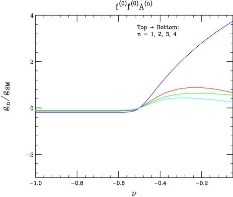
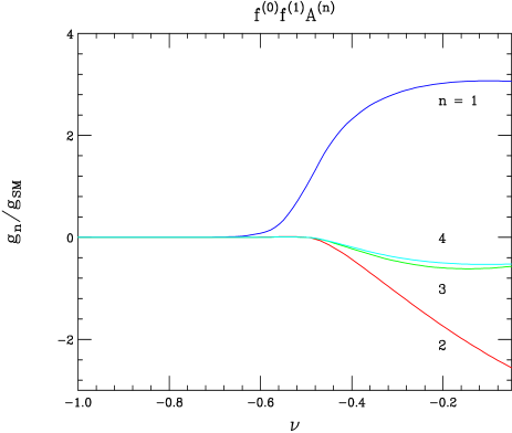
Figure 1: The coefficients $C^{00n}_{f\bar{f}A}$ (left) and $C^{01n}_{f\bar{f}A}$ (right) for $n=1,\ldots,4$ as functions of the fermion bulk mass parameter $\nu$.

We will also require the couplings between gauge KK states and the fermion fields which are localized on the TeV-brane [4]. The relevant action is

$$S_{F}=\int d^{4}x\int d\phi\sqrt{-G}\left[V^{M}_{n}\left(\frac{i}{2}\bar{\psi}\gamma^{n}\stackrel{{\scriptstyle\leftrightarrow}}{{D}}_{M}\psi+{\rm h.c.}\right)\right]\delta\left(\phi-\pi\right)\,\,.$$ (14)

Inserting the expansion of Eq. 5 into this expression, letting $\psi\rightarrow e^{3\sigma/2}\psi$, and setting $g=g_{5}/\sqrt{2\pi r_{c}}$, we find that the ratio of the n^th KK gauge coupling to localized fermions relative to the corresponding SM coupling is

$$C^{n}_{f\bar{f}A}=\frac{\chi^{(n)}(\pi)}{\chi^{(0)}(\pi)}\,\,.$$ (15)

Utilizing the approximate expressions for the KK gauge wavefunctions in [9], these become

$$C^{n}_{f\bar{f}A}\approx\left(-1\right)^{n+1}\sqrt{2\pi kr_{c}}\,\,.$$ (16)

We now consider the final ingredient required for construction of the SM, the Higgs boson. As discussed in the introduction, the Higgs field must be confined to the TeV-brane to correctly break the electroweak symmetry. Its action can therefore be expressed as

$$S_{H}=\int d^{4}x\int dy\sqrt{-G}\left\{G^{MN}D_{M}H\left(D_{N}H\right)^{\dagger}-V(H)\right\}\delta(y-r_{c}\pi)\,\,,$$ (17)

where $V(H)$ is the Higgs potential and $D_{M}$ the covariant derivative. To properly normalize the Higgs field kinetic term we must rescale $H\rightarrow e^{\sigma}H$; we then expand $H$ around its vev, $v$, insert the expansion of Eq. 5 into the covariant derivative, and identify $g=g_{5}/\sqrt{2\pi r_{c}}$. We find the gauge field mass terms

$$S_{H,mass}=\frac{1}{2}\sum_{m,n=0}^{\infty}a_{mn}\int d^{4}x\,m_{A,0}^{2}\,A^{(m)}_{\mu}A^{(n),\mu}\,\,,$$ (18)

where $m_{A,0}$ is the gauge field mass of the 4-dimensional theory corresponding to the zero-mode of the gauge KK tower, and

$$a_{mn}=2\pi\chi^{(m)}(\pi)\chi^{(n)}(\pi)\,\,.$$ (19)

We must diagonalize the full mass matrix, including the contributions arising from the KK reduction, to obtain the physical spectrum; we will do so for the SM gauge fields in a later section.

We now examine the mixing between fermion KK states induced by the Higgs field. When fermion fields are confined to the TeV-brane, no such mixing occurs; we therefore consider only the case where the fermions propagate in the bulk. The coupling between the Higgs and KK fermions is

$$S_{f\bar{f}H}=\frac{\lambda^{{}^{\prime}}}{k}\int d^{4}x\int dy\sqrt{-G}\left\{H^{\dagger}\Psi_{D}\Psi^{c}_{S}+{\rm h.c.}\right\}\delta\left(y-r_{c}\pi\right)\,\,,$$ (20)

where $\lambda^{{}^{\prime}}$ is the 5-dimensional Yukawa coupling, and $k$ has been introduced to make $\lambda^{{}^{\prime}}$ dimensionless. Both $\Psi_{D}$ and $\Psi^{c}_{S}$ are left-handed Weyl fermions; we have introduced the subscripts $D$ and $S$ for these fields to indicate that in the SM, the Higgs couples $SU(2)_{L}$ doublets to $SU(2)_{L}$ singlets. After diagonalization of the mass matrix, the hermitian conjugates of the singlet fields will combine with the appropriate doublets to form Dirac fermions. Since, for our analysis, we are interested only in the contributions to the fermion masses arising from this action, we again rescale the Higgs field by $e^{\sigma}$, set the Higgs field equal to its vev and expand the left-handed fermion wavefunctions as in Eq. 9. Identifying

$$\lambda=\frac{\lambda^{{}^{\prime}}\left(f^{(0)}_{L}(\pi)\right)^{2}e^{kr_{c}\pi}}{kr_{c}}$$ (21)

as the 4-dimensional Yukawa coupling, we find the fermion mass terms

$$S_{f,mass}=\sum_{m,n=0}^{\infty}b_{mn}\int d^{4}x\left\{m_{f,0}\psi^{(m)}_{D}\psi^{c,(n)}_{S}+{\rm h.c.}\right\}\,\,,$$ (22)

where $m_{f,0}$ is the zero mode mass obtained when the KK states decouple, and

$$b_{mn}=\frac{f^{(m)}_{L}(\pi)f^{(n)}_{L}(\pi)}{\left(f^{(0)}_{L}(\pi)\right)^{2}}\,\,.$$ (23)

Since $f^{(n)}_{L}(\pi)$ is approximately the same function for all $n\geq 1$, we will set $b_{0n}=\sqrt{f}$ and $b_{mn}=f$, with $m\neq n\neq 0$, in our analysis, where $f$ is a $\nu$ dependent quantity that measures the strength of the mixing. This parameter is explicitly given by

$$f=2{1-e^{-k\pi r_{c}(1+2\nu)}\over 1+2\nu}\,.$$ (24)

These mass terms must be diagonalized in conjunction with the contributions from the KK reduction of Eq. 8; we will do so for the SM $b$ and $t$ quarks in the next section.

To complete our discussion of the RS model, we must briefly discuss the KK gravitons it contains. We parameterize the 5-dimensional metric as

$$G_{\alpha\beta}=e^{-2\sigma}\left(\eta_{\alpha\beta}+\kappa_{5}h_{\alpha\beta}\right)\,\,,$$ (25)

where $\kappa_{5}=2M_{5}^{-3/2}$, $\eta_{\alpha\beta}$ is the Minkowski metric with signature -2, and the fluctuations of the bulk radius have been neglected. We then expand the graviton field $h_{\alpha\beta}$ as

$$h_{\alpha\beta}(x,\phi)=\sum_{n=0}^{\infty}h^{(n)}_{\alpha\beta}(x)\frac{\chi^{n}_{G}(\phi)}{\sqrt{r_{c}}}\,\,,$$ (26)

and impose the orthonormality constraint

$$\int_{-\pi}^{\pi}d\phi\,e^{-2\sigma}\chi^{(m)}_{G}\chi^{(n)}_{G}=\delta^{mn}\,\,.$$ (27)

The explicit forms of the KK graviton wavefunctions contain the second order Bessel functions $J_{2}$ and $Y_{2}$, and can be found in [3, 9]. Expressing the graviton masses as $m^{G}_{n}=x^{G}_{n}ke^{-kr_{c}\pi}$, we find the numerical values $x^{G}_{1}\simeq 3.83$, $x^{G}_{2}\simeq 7.02$, $x^{G}_{3}\simeq 10.17$ for the first few states which are given by $J_{1}(x_{n}^{G})=0$; notice that $m^{G}_{n}>m^{A}_{n}$. The couplings of the KK gravitons to fermions are given by

$$C^{mnq}_{f\bar{f}G}=\int_{-\pi}^{\pi}d\phi\frac{e^{\sigma}f^{(m)}f^{(n)}\chi^{(q)}_{G}}{\sqrt{kr_{c}}}\,\,.$$ (28)

The $C^{00n}_{f\bar{f}G}$ are presented in Fig. 2 as functions of $\nu$. These couplings are relatively small, particularly when $\nu\leq-0.5$; this, and their large mass, render the KK gravitons unimportant in our analysis.

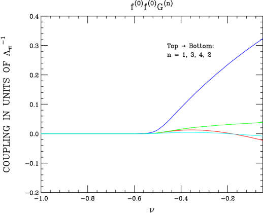
Figure 2: The coupling strengths $C^{00n}_{f\bar{f}G}$ for $n=1,\ldots,4$ as functions of the fermion bulk mass parameter $\nu$ in units of $\Lambda_{\pi}$.

We now have the tools necessary to build the SM within the RS framework. In the next section we will discuss the diagonalization of the $t$ and $b$ quark mass matrices, and the KK contributions to the $\rho$ parameter. To whet the reader’s appetite, we note that the off-diagonal mass matrix elements $b_{mn}$, with $m,n\neq 1$ and $m\neq n$, range from $\approx 10$ when $\nu=-0.4$ to $\approx 700$ when $\nu=-0.6$. This induces large mixing between the zero mode top quark and its KK tower, and creates couplings between the zero mode $b$ quark and the top quark KK states. The large mass splitting between these states results in drastic alterations of $\rho$, and renders the placement of third generation quarks in the bulk inconsistent with EW measurements for a wide range of KK masses.

3 Fermion Mixing and the $\rho$ Parameter

Since the top quark is quite heavy, with a mass $m_{t}\approx 175$ GeV, we expect the mixing between it and its KK tower to be stronger than that for the lighter fermions, and we focus here upon it and its isodoublet partner, the bottom quark. As mentioned previously, after performing the KK reduction of the 5-dimensional fermion field we obtain a chiral zero mode and a vector-like KK tower; this spectrum is presented pictorially for the top quark in Table 1.

Doublet		Singlet
⋮	⋮	⋮	⋮
$T^{(2)}_{L}$	$T^{(2)}_{R}$	$t^{(2)}_{L}$	$t^{(2)}_{R}$
$T^{(1)}_{L}$	$T^{(1)}_{R}$	$t^{(1)}_{L}$	$t^{(1)}_{R}$
$T^{(0)}_{L}$	$X$	$X$	$t^{(0)}_{R}$

Table 1: Abbreviated list of the top quark KK states. The subscripts $L$ and $R$ denote left-handed and right-handed fields. $SU(2)_{L}$ doublets are denoted by capital $T$ and singlets by lower case $t$. An $X$ at a location in the table indicates that the state does not exist due to the orbifold symmetry.

We have exchanged the left-handed $SU(2)_{L}$ Weyl singlets introduced in the preceding section for their right-handed conjugates, but the reader should remember that these states are still described by the 5-dimensional wavefunctions $f^{(n)}_{L}(\phi)$. The top quark mass matrix receives two distinct contributions: the diagonal KK couplings between the doublet tower states and the singlet tower states, and off-diagonal mixings between the left-handed doublets and right-handed singlets arising from the Higgs coupling on the TeV-brane. We present below the mass matrix with only the zero modes and the first two KK levels included; the infinite-dimensional case can be obtained by a simple generalization. Working in the weak eigenstate basis defined by the vectors $\Psi^{t}_{L}=\left(T^{(0)}_{L},T^{(1)}_{L},t^{(1)}_{L},T^{(2)}_{L},t^{(2)}_{L}\right)$ and $\Psi^{t}_{R}=\left(t^{(0)}_{R},t^{(1)}_{R},T^{(1)}_{R},t^{(2)}_{R},T^{(2)}_{R}\right)$, we find

$${\cal M}_{t}=\left(\begin{array}[]{ccccc}m_{t,0}&\sqrt{f}m_{t,0}&0&-\sqrt{f}m_{t,0}&0\\ \sqrt{f}m_{t,0}&fm_{t,0}&m_{1}&-\sqrt{f}m_{t,0}&0\\ 0&m_{1}&0&0&0\\ -\sqrt{f}m_{t,0}&-fm_{t,0}&0&fm_{t,0}&m_{2}\\ 0&0&0&m_{2}&0\end{array}\right)\,\,.$$ (29)

$m_{t,0}$ is the mass of the zero mode in the infinite KK mass limit, and $m_{1}$ and $m_{2}$ are the masses of the first two KK fermion states in the limit of vanishing Higgs couplings; $f$ is the mixing strength introduced in the previous section. We fix $m_{t,0}$ by demanding that the lowest lying eigenvalue of this matrix reproduce the measured top quark mass, $m_{t}=174.3$ GeV. Due to the large values of the off-diagonal elements, we diagonalize this mass matrix numerically, rather than analytically to ${\cal O}(m_{t,0}/m_{1})$. We must necessarily truncate the KK expansion at some level; we have performed our analysis twice, once including only the first KK level and once keeping the first two levels, and have checked that adding more states only strengthens our conclusions. We examine the parameter region $-0.3\mathrel{\mathchoice{\lower 3.01385pt\vbox{\halign{$\matth\displaystyle\hfil#\hfil$\cr>\crcr\sim\crcr}}}{\lower 3.01385pt\vbox{\halign{$\matth\textstyle\hfil#\hfil$\cr>\crcr\sim\crcr}}}{\lower 3.01385pt\vbox{\halign{$\matth\scriptstyle\hfil#\hfil$\cr>\crcr\sim\crcr}}}{\lower 3.01385pt\vbox{\halign{$\matth\scriptscriptstyle\hfil#\hfil$\cr>\crcr\sim\crcr}}}}\nu\mathrel{\mathchoice{\lower 3.01385pt\vbox{\halign{$\matth\displaystyle\hfil#\hfil$\cr>\crcr\sim\crcr}}}{\lower 3.01385pt\vbox{\halign{$\matth\textstyle\hfil#\hfil$\cr>\crcr\sim\crcr}}}{\lower 3.01385pt\vbox{\halign{$\matth\scriptstyle\hfil#\hfil$\cr>\crcr\sim\crcr}}}{\lower 3.01385pt\vbox{\halign{$\matth\scriptscriptstyle\hfil#\hfil$\cr>\crcr\sim\crcr}}}}-0.55$; the range $\nu>-0.3$ is strongly constrained by contact interaction searches at LEP [9], and the values $\nu\mathrel{\mathchoice{\lower 3.01385pt\vbox{\halign{$\matth\displaystyle\hfil#\hfil$\cr<\crcr\sim\crcr}}}{\lower 3.01385pt\vbox{\halign{$\matth\textstyle\hfil#\hfil$\cr<\crcr\sim\crcr}}}{\lower 3.01385pt\vbox{\halign{$\matth\scriptstyle\hfil#\hfil$\cr<\crcr\sim\crcr}}}{\lower 3.01385pt\vbox{\halign{$\matth\scriptscriptstyle\hfil#\hfil$\cr<\crcr\sim\crcr}}}}-0.55$ are prohibited by extrapolation of the results obtained below. This is essentially the same region studied in [13, 14], where it was shown that the LHC will be able to probe the shift in the $Zt\bar{t}$ coupling for fermion KK mass values $m_{1}\mathrel{\mathchoice{\lower 3.01385pt\vbox{\halign{$\matth\displaystyle\hfil#\hfil$\cr<\crcr\sim\crcr}}}{\lower 3.01385pt\vbox{\halign{$\matth\textstyle\hfil#\hfil$\cr<\crcr\sim\crcr}}}{\lower 3.01385pt\vbox{\halign{$\matth\scriptstyle\hfil#\hfil$\cr<\crcr\sim\crcr}}}{\lower 3.01385pt\vbox{\halign{$\matth\scriptscriptstyle\hfil#\hfil$\cr<\crcr\sim\crcr}}}}15$ TeV. We will find that the region where $\nu\leq-0.3$ and $m_{1}\mathrel{\mathchoice{\lower 3.01385pt\vbox{\halign{$\matth\displaystyle\hfil#\hfil$\cr<\crcr\sim\crcr}}}{\lower 3.01385pt\vbox{\halign{$\matth\textstyle\hfil#\hfil$\cr<\crcr\sim\crcr}}}{\lower 3.01385pt\vbox{\halign{$\matth\scriptstyle\hfil#\hfil$\cr<\crcr\sim\crcr}}}{\lower 3.01385pt\vbox{\halign{$\matth\scriptscriptstyle\hfil#\hfil$\cr<\crcr\sim\crcr}}}}30-100$ TeV is already disfavoured by current measurements.

The Lagrangian containing the top quark mass terms and its interactions with the $Z$ and $W^{\pm}$ gauge bosons is

$${\cal L} = \left(\bar{\Psi}^{t}_{L}{\cal M}_{t}\Psi^{t}_{R}+{\rm h.c.}\right)+\bar{\Psi}^{t}_{L}\not\!{Z}C^{Z}_{t,L}\Psi^{t}_{L}+\bar{\Psi}^{t}_{R}\not\!{Z}C^{Z}_{t,R}\Psi^{t}_{R}$$ (30)

$$+\bar{\Psi}^{t}_{L}\not\!{W}^{-}C^{W}_{L}\Psi^{b}_{L}+\bar{\Psi}^{t}_{R}\not\!{W}^{-}C^{W}_{R}\Psi^{b}_{R}+\,...+{\rm h.c.}\,\,.$$

We have introduced the basis $\Psi^{b}_{L}$ and $\Psi^{b}_{R}$ for the bottom quark in analogy with those for the top quark. The $C^{i}_{j}$ are matrices containing the couplings of the various top quark states to the $Z$ and $W^{\pm}$; letting $g$ denote the SM electroweak coupling, $c_{W}$ the cosine of the weak mixing angle, and $g_{L}$ and $g_{R}$ the couplings of the usual left-handed and right-handed SM fermions to the $Z$ boson, we find

$$C^{Z}_{t,L} = \frac{g}{c_{W}}\,{\rm diag}\left(g_{L},g_{L},g_{R},g_{L},g_{R}\right)\,\,,$$

$$C^{Z}_{t,R} = \frac{g}{c_{W}}\,{\rm diag}\left(g_{R},g_{R},g_{L},g_{R},g_{L}\right)\,\,,$$

$$C^{W}_{L} = \frac{g}{\sqrt{2}}\,{\rm diag}\left(1,1,0,1,0\right)\,\,,$$

$$C^{W}_{R} = \frac{g}{\sqrt{2}}\,{\rm diag}\left(0,0,1,0,1\right)\,\,.$$ (31)

In obtaining these matrices we have treated the $T^{(n)}_{R}$ as $SU(2)_{L}$ doublets and the $t^{(n)}_{L}$ as singlets as denoted in Table 1. We diagonalize ${\cal M}_{t}$ with the two unitary matrices $U^{t}_{L}$ and $U^{t}_{R}$,

$${\cal M}^{D}_{t}=U^{t}_{L}{\cal M}_{t}\left(U^{t}_{R}\right)^{\dagger}\,\,.$$ (32)

Diagonalization of the matrix ${\cal M}_{t}{\cal M}^{\dagger}_{t}$ determines $U^{t}_{L}$ up to an overall phase matrix, while diagonalization of ${\cal M}^{\dagger}_{t}{\cal M}_{t}$ similarly fixes $U^{t}_{R}$. The mass eigenstate basis is obtained by multiplication of the weak eigenstate basis by the appropriate transformation matrix:

$$\Psi^{t}_{L}\rightarrow U^{t}_{L}\Psi^{t}_{L}\,\,\,\,,\Psi^{t}_{R}\rightarrow U^{t}_{R}\Psi^{t}_{R}\,\,.$$ (33)

The coupling matrices undergo a similar shift,

$$C^{Z}_{t,L} \rightarrow U^{t}_{L}C^{Z}_{t,L}\left(U^{t}_{L}\right)^{\dagger}\,\,,$$

$$C^{Z}_{t,R} \rightarrow U^{t}_{R}C^{Z}_{t,R}\left(U^{t}_{R}\right)^{\dagger}\,\,,$$

$$C^{W}_{L} \rightarrow U^{t}_{L}C^{W}_{L}\left(U^{b}_{L}\right)^{\dagger}\,\,,$$

$$C^{W}_{R} \rightarrow U^{t}_{R}C^{W}_{R}\left(U^{b}_{R}\right)^{\dagger}\,\,.$$ (34)

We have also implicitly performed an identical diagonalization of the bottom quark mass matrix.

This procedure induces off-diagonal elements in both the $Z$ and $W^{\pm}$ coupling matrices; consequently, fermions of widely varying masses enter the vacuum polarization graphs contributing to the $Z$ and $W^{\pm}$ self energies. Such a scenario typically generates unacceptable contributions to the $\rho$ parameter [15], defined as

$$\rho=\frac{\Pi_{W}\left(q^{2}=0\right)}{M_{W}^{2}}-\frac{\Pi_{Z}\left(q^{2}=0\right)}{M_{Z}^{2}}\,\,,$$ (35)

where $\Pi_{X}\left(q^{2}\right)$ is the $X$ boson self energy function. We set $\Delta\rho=\rho-\rho_{SM}$, where $\rho_{SM}$ is the contribution from the SM $(t,b)$ doublet, and calculate $\rho$ for our two cases: once including the shifted top and bottom quark zero modes and the first KK level only, and once including the zero modes and the first two KK states. $\Delta\rho$ is then a measure of the deviation from the SM prediction. The results are presented in Fig. 3 as functions of $\nu$ for several choices of $m_{1}$. The 95% CL exclusion limit [16] of $\Delta\rho\mathrel{\mathchoice{\lower 3.01385pt\vbox{\halign{$\matth\displaystyle\hfil#\hfil$\cr<\crcr\sim\crcr}}}{\lower 3.01385pt\vbox{\halign{$\matth\textstyle\hfil#\hfil$\cr<\crcr\sim\crcr}}}{\lower 3.01385pt\vbox{\halign{$\matth\scriptstyle\hfil#\hfil$\cr<\crcr\sim\crcr}}}{\lower 3.01385pt\vbox{\halign{$\matth\scriptscriptstyle\hfil#\hfil$\cr<\crcr\sim\crcr}}}}2\times 10^{-3}$ is also indicated. Notice that $\Delta\rho$ increases when we add the second KK level in our analysis; thus adding more states only increases $\Delta\rho$ further, and our neglect of these higher modes is justified. It is clear from the lower graph in Fig. 3 that consistency with the 95% CL exclusion limit restricts $m_{1}$ to the range $m_{1}\mathrel{\mathchoice{\lower 3.01385pt\vbox{\halign{$\matth\displaystyle\hfil#\hfil$\cr>\crcr\sim\crcr}}}{\lower 3.01385pt\vbox{\halign{$\matth\textstyle\hfil#\hfil$\cr>\crcr\sim\crcr}}}{\lower 3.01385pt\vbox{\halign{$\matth\scriptstyle\hfil#\hfil$\cr>\crcr\sim\crcr}}}{\lower 3.01385pt\vbox{\halign{$\matth\scriptscriptstyle\hfil#\hfil$\cr>\crcr\sim\crcr}}}}25$ TeV for all values of $\nu$ in the previously allowed range, and requires $m_{1}\mathrel{\mathchoice{\lower 3.01385pt\vbox{\halign{$\matth\displaystyle\hfil#\hfil$\cr>\crcr\sim\crcr}}}{\lower 3.01385pt\vbox{\halign{$\matth\textstyle\hfil#\hfil$\cr>\crcr\sim\crcr}}}{\lower 3.01385pt\vbox{\halign{$\matth\scriptstyle\hfil#\hfil$\cr>\crcr\sim\crcr}}}{\lower 3.01385pt\vbox{\halign{$\matth\scriptscriptstyle\hfil#\hfil$\cr>\crcr\sim\crcr}}}}100$ TeV when $\nu\leq-0.4$. When $\nu<-0.5$, including the range $\nu\leq-0.55$ that we have not presented, the corrections to $\rho$ are so large that the perturbative definition of the $Z$ and $W^{\pm}$ gauge bosons is no longer valid. We stress that these restrictions are lower bounds on the actual constraints as including more KK levels in our analysis will only strengthen these results. These results imply $\Lambda_{\pi}\mathrel{\mathchoice{\lower 3.01385pt\vbox{\halign{$\matth\displaystyle\hfil#\hfil$\cr>\crcr\sim\crcr}}}{\lower 3.01385pt\vbox{\halign{$\matth\textstyle\hfil#\hfil$\cr>\crcr\sim\crcr}}}{\lower 3.01385pt\vbox{\halign{$\matth\scriptstyle\hfil#\hfil$\cr>\crcr\sim\crcr}}}{\lower 3.01385pt\vbox{\halign{$\matth\scriptscriptstyle\hfil#\hfil$\cr>\crcr\sim\crcr}}}}100$ TeV [4], with the exact choice depending on the value of $\nu$, to avoid unacceptable contributions to $\Delta\rho$; the resulting hierarchy between the EW scale and the fundamental RS scale thus strongly disfavors allowing the third generation quarks to propagate in the bulk.

This restriction applies only to the top and bottom quarks; the first and second generations are much less massive, and the large mixing induced above by the top quark Yukawa coupling does not appear when considering these states. We have numerically checked that the contributions of bulk first and second generation quarks are consistent with the constraints on $\Delta\rho$, and hence the placement of the first two generations in the bulk is still allowed. But, is such a setup motivated? Does any interesting physics result from this construction? The answer to both questions is unequivocally yes, as we will demonstrate in the next section.

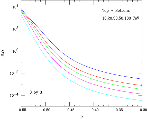
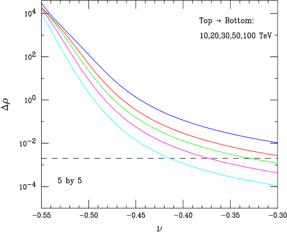
Figure 3: Contributions to $\Delta\rho$ from the zero modes and first KK level (top), and from the zero modes and first two KK levels (bottom). The dashed black line indicates where $\Delta\rho=2\times 10^{-3}$. The various curves correspond to when the masses of the first fermion KK excitation is taken to be $m_{1}=10,20,30,50,100$ TeV, from top to bottom.

4 The Third Generation On the Wall and the EW Precision Observables

A handful of authors have attempted to construct models explaining the quark and neutrino mass matrices within the framework of the RS model [7, 8]. These ideas generically require the placement of fermions at different locations in the 5-dimensional bulk. We have already shown that the third generation quarks must lie on the TeV-brane; if we permit the first two generations to propagate in the bulk, can we explain the hierarchy between the Yukawa coupling of the top quark and those of the lighter quarks?

We consider first the coupling of the Higgs to a fermion field confined to the TeV-brane; the relevant action is

$$S^{wall}_{f\bar{f}H}=\lambda^{wall}\int d^{4}x\int dy\sqrt{-G}\left\{H^{\dagger}\psi_{D}\psi^{c}_{S}+{\rm h.c.}\right\}\delta\left(y-r_{c}\pi\right)\,\,,$$ (36)

where $\lambda^{wall}$ is the Yukawa coupling of the localized fermion, chosen to be of ${\cal O}(1)$. To derive the 4-dimensional action we must rescale $\psi\rightarrow e^{3\sigma/2}\psi$ and $H\rightarrow e^{\sigma}H$ as before. The mass of this field is then $m^{wall}=\lambda^{wall}v/\sqrt{2}$. We have shown in Eq. 21 that the 4-d Yukawa coupling that determines the zero-mode mass of a bulk fermion is

$$\lambda^{bulk}=\frac{\lambda^{{}^{\prime}}\left(f^{(0)}_{L}(\pi)\right)^{2}e^{kr_{c}\pi}}{kr_{c}}\,\,.$$ (37)

We now assume that the fundamental coupling that enters the 5-d bulk fermion action, $\lambda^{{}^{\prime}}$, is also of order unity as is $\lambda^{wall}$. The factor $\left(f^{(0)}_{L}\right)^{2}e^{kr_{c}\pi}/kr_{c}$ then suppresses $\lambda^{bulk}$ with respect to $\lambda^{wall}$; we find $\lambda^{bulk}\approx\left(10^{-1}-10^{-2}\right)\lambda^{wall}$ when $-0.55\mathrel{\mathchoice{\lower 3.01385pt\vbox{\halign{$\matth\displaystyle\hfil#\hfil$\cr<\crcr\sim\crcr}}}{\lower 3.01385pt\vbox{\halign{$\matth\textstyle\hfil#\hfil$\cr<\crcr\sim\crcr}}}{\lower 3.01385pt\vbox{\halign{$\matth\scriptstyle\hfil#\hfil$\cr<\crcr\sim\crcr}}}{\lower 3.01385pt\vbox{\halign{$\matth\scriptscriptstyle\hfil#\hfil$\cr<\crcr\sim\crcr}}}}\nu\mathrel{\mathchoice{\lower 3.01385pt\vbox{\halign{$\matth\displaystyle\hfil#\hfil$\cr<\crcr\sim\crcr}}}{\lower 3.01385pt\vbox{\halign{$\matth\textstyle\hfil#\hfil$\cr<\crcr\sim\crcr}}}{\lower 3.01385pt\vbox{\halign{$\matth\scriptstyle\hfil#\hfil$\cr<\crcr\sim\crcr}}}{\lower 3.01385pt\vbox{\halign{$\matth\scriptscriptstyle\hfil#\hfil$\cr<\crcr\sim\crcr}}}}-0.35$, using the zero mode wavefunction given in Eq. 11. Choosing a value of $\nu$ in this region, ameliorates the hierarchy between the second and third generation quark Yukawa couplings. To be more explicit, with the top quark on the TeV brane and $\lambda^{wall}$ of order unity, we expect a top mass near its experimental value. On the other hand, for the charm quark in the bulk, we expect a much smaller mass even if the bulk Yukawa coupling $\lambda^{\prime}$ is also of order unity. As an example, assuming $\lambda^{\prime}=\lambda^{wall}$ and taking $\nu=-0.5$ one obtains $m_{t}/m_{c}\simeq 2\pi kr_{c}\simeq 70$ which is within a factor of 2 to 3 of the experimental value. A similar argument applies to the $m_{b}/m_{s}$ ratio. The localization of the third generation on the TeV brane while keeping the first two in the bulk may thus help explain the fermion mass hierarchy. We do not attempt here to build a more detailed flavor model incorporating the off-diagonal CKM matrix elements, but instead examine the consequences of this simple situation. We focus on the region $-0.6\leq\nu\leq-0.3$, extending slightly for completeness the range preferred by the quark Yukawa hierarchy. We study next the effects of KK gauge boson mixing on the EW precision observables; we will find that large mixing similar to that appearing in the top quark mass matrix relaxes the upper bound on the Higgs boson mass obtained in the standard EW fit [17].

The mass terms for the $W^{\pm}$ and $Z$ can be obtained using Eq. 18 as a template; we find

$$S_{mass}=\sum_{m,n=0}^{\infty}a_{mn}\int d^{4}x\left(m_{W,0}^{2}W^{+(m)}_{0}W^{-(n)}_{0}+\frac{1}{2}m_{Z,0}^{2}Z^{(m)}_{0}Z^{(n)}_{0}\right)\,\,,$$ (38)

where the $a_{mn}$ are given by Eq. 19 and we have for notational simplicity omitted the Lorentz indices of the gauge fields. The resulting $W^{\pm}$ mass matrix is

$${\cal M}_{W}^{2}=m_{1}^{2}\left(\begin{array}[]{cccc}a_{11}x_{W}&a_{12}x_{W}&a_{13}x_{W}&\ldots\\ a_{12}x_{W}&b_{1}^{2}+a_{22}x_{W}&a_{23}x_{W}&\ldots\\ a_{13}x_{W}&a_{23}x_{W}&b_{2}^{2}+a_{33}x_{W}&\ldots\\ \vdots&\vdots&\vdots&\end{array}\right)\,\,,$$ (39)

where $m_{1}$ is the first KK gauge mass, $x_{W}=m_{W,0}^{2}/m_{1}^{2}$, and $b_{i}=m_{i}/m_{1}$ is the ratio of the $i$th KK mass to the first. The mass matrix for the $Z$ is obtained by substituting $m_{W,0}\rightarrow m_{Z,0}$. The subscripts on the fields $W^{\pm}_{0}$ and $Z_{0}$, and on the masses $m_{W,0}$ and $m_{Z,0}$, indicate that these are not the physical fields and masses; they are the zero-mode fields and masses in the infinite KK limit. To obtain the physical spectrum we must diagonalize the mass matrices while respecting the appropriate constraints; these are the same as those developed for the interpretation of precision measurements at the $Z$-pole [18]. This prescription states that the following quantities are inputs to radiative corrections and to fits to the precision EW data: $\alpha$ as measured in Thomson scattering, $G_{F}$ as defined by the muon lifetime, $M_{Z}$ as determined from the $Z$ line shape, $m_{t}$ as measured at the Tevatron, and $m_{H}$, which is currently a free parameter. All other observables, such as the $W^{\pm}$ mass, $M_{W}$, and the width for the decay $Z\rightarrow l^{+}l^{-}$, $\Gamma_{l}$, are derived from these measured quantities; we must compare the RS model predictions for these parameters with the values obtained by experiment.

We examine the six relatively uncorrelated observables $M_{W}$, ${\rm sin}^{2}\theta_{\rm eff}$, $\Gamma_{l}$, $R_{b}$, $R_{c}$, and ${\rm sin}^{2}\theta_{\rm\nu N}$, and discuss in detail our procedure for deriving the RS model predictions for these quantities and then compare these predictions to the measured values. We consider tree level KK and loop level SM contributions to these observables, and assume that contributions from KK loops are higher order and therefore negligible. Our analysis differs slightly from those performed in models with KK gauge bosons arising from ${\rm TeV}^{-1}$-sized extra dimensions [19, 20]. Here, the parameters $a_{mn}$ of Eq. 19 which enter the mass matrices are rather large; the $a_{1n}$, with $n>1$, have the approximate value $\sqrt{2\pi kr_{c}}\approx 8.4$, while the elements $a_{mn}$, with $m,n>1$ and $m\neq n$, have the approximate value $2\pi kr_{c}\approx 71$. Although the ratios $x_{W(Z)}=m_{W,0(Z,0)}^{2}/m_{1}^{2}$ that appear in the mass matrices may be small, they are multiplied by these large coefficients, and to avoid errors we diagonalize the matrices and handle shifts of the precision observables numerically to all orders in $x_{W,Z}$, rather than performing the analysis analytically to ${\cal O}(x_{W,Z})$. This necessitates a truncation of the mass matrices; we work with $30\times 30$ matrices, and have verified that increasing the size to $60\times 60$ produces a negligible change in our results.

We first determine the parameter $m_{Z,0}$ by diagonalizing the $Z$ mass matrix and demanding that the lowest eigenvalue reproduce the measured $Z$ mass, $M_{Z}$ . Armed with $m_{Z,0}$, we consider next the muon lifetime, through which the input parameter $G_{F}$ is defined. The relevant decay is $\mu^{-}\rightarrow e^{-}\nu_{e}\bar{\nu}_{\mu}$. In the SM this proceeds at tree level through $W$ exchange; it proceeds here through the exchange of the entire $W^{(n)}$ KK tower. $G_{F}$ therefore becomes

$$\frac{G_{F}}{\sqrt{2}}=\frac{g^{2}}{8M_{W}^{2}}+\frac{g_{0}^{2}}{8}\sum_{n}\frac{c_{n}}{m_{n}^{2}}\,\,,$$ (40)

where the first term arises from the exchange of the zero mode and the second term from the higher KK states, and the $c_{n}$ encapsulate the couplings of the KK gauge states to zero mode leptons. Some clarification of this expression is required. $g$ is the coupling of the physical $W$ obtained after diagonalization, whereas $g_{0}$ is the coupling that appears in the Lagrangian before diagonalization. To make this distinction explicit we express $g$ as

$$g=g_{0}\left\{1-G(m_{W,0})\right\}\,\,,$$ (41)

where $G(m_{W,0})$ accounts for the admixture of KK states in the physical $W^{(0)}$ boson. After EW symmetry breaking, $g_{0}^{2}=4\pi\alpha/s_{w,0}^{2}$, where $s_{w,0}$ is the sine of the weak mixing angle obtained before including mixing effects: $s_{w,0}^{2}=1-m_{W,0}^{2}/m_{Z,0}^{2}$. Substituting these relations into Eq. 40, we arrive at the condition

$$1=\frac{\pi\alpha}{\sqrt{2}G_{F}\,M_{W}^{2}s_{w,0}^{2}}\left\{1-G(m_{W,0})\right\}^{2}+\frac{\pi\alpha}{\sqrt{2}s_{w,0}^{2}}H(m_{W,0})\,\,,$$ (42)

where we have introduced the dimensionless quantity

$$H(m_{W,0})=\frac{1}{G_{F}}\sum_{n}\frac{c_{n}}{m_{n}^{2}}\,\,.$$ (43)

In the SM, after radiative corrections are included,

$$\frac{\pi\alpha}{\sqrt{2}G_{F}}\rightarrow\frac{\pi\alpha}{\sqrt{2}G_{F}\left(1-\Delta r\right)}=m_{W,SM}^{2}\left[1-\frac{m_{W,SM}^{2}}{M_{Z}^{2}}\right]\,\,.$$ (44)

To incorporate radiative corrections in our analysis, we make this substitution in Eq. 42, and use the $m_{W,SM}$ calculated by ZFITTER [21] using $M_{Z}$ as an input. We find the relation

$$1=\frac{m_{W,SM}^{2}\left[1-\frac{m_{W,SM}^{2}}{M_{Z}^{2}}\right]}{M_{W}^{2}\left[1-\frac{M_{W}^{2}}{M_{Z}^{2}}\right]}\left\{1-G(m_{W,0})\right\}^{2}+\frac{\pi\alpha}{\sqrt{2}\left(1-\frac{m_{W,0}^{2}}{m_{Z,0}^{2}}\right)}H(m_{W,0})\,\,.$$ (45)

The only unknown quantity in this equation is $m_{W,0}$; the physical $W^{\pm}$ mass, $M_{W}$, is derived from $m_{W,0}$ through diagonalization of the $W^{\pm}$ mass matrix. We now scan over $m_{W,0}$ until we find a solution to this equation; the $m_{W,0}$ that furnishes this solution also predicts a $M_{W}$ that can be compared with experiment.

We next compute the KK contributions to the effective coupling ${\rm sin}^{2}\theta_{eff}$, which appears in the dressed $Zl^{+}l^{-}$ vertex [21]. In the SM,

$${\rm sin}^{2}\theta_{eff,SM}=\kappa^{Z}{\rm sin}^{2}\theta_{w,SM}\,\,,$$ (46)

where $\theta_{w}$ is the on-shell weak mixing angle, ${\rm sin}^{2}\theta_{w,SM}=1-m_{W,SM}^{2}/M_{Z}^{2}$, and $\kappa^{Z}$ contains a subset of the radiative corrections to the decay $Z\rightarrow l^{+}l^{-}$. In the RS model, the weak mixing angle that appears in the $Zl^{+}l^{-}$ vertex is $s_{w,0}$; this is unaffected by diagonalization because $s_{w,0}$ enters the coupling of every KK excitationstate. The RS model expression for ${\rm sin}^{2}\theta_{eff}$ is

$${\rm sin}^{2}\theta_{eff}=\kappa^{Z}s_{w,0}^{2}={\rm sin}^{2}\theta_{eff,SM}\left(\frac{1-\frac{m_{W,0}^{2}}{m_{Z,0}^{2}}}{1-\frac{m_{W,SM}^{2}}{M_{Z}^{2}}}\right)\,\,,$$ (47)

where in the last step we have incorporated the ZFITTER predictions for ${\rm sin}^{2}\theta_{eff,SM}$ and $m_{W,SM}$ to correctly account for the SM radiative corrections.

The shifts of the remaining observables occur in a similar fashion as in the two examples given above, and hence we discuss them only briefly here. The width of the decay $Z\rightarrow\bar{f}f$ is

$$\Gamma_{f}=\frac{g^{2}M_{Z}}{96\pi c_{w}^{2}}C_{f}\left\{\left[1-4|Q_{f}|{\rm sin}^{2}\theta_{eff}+8Q_{f}^{2}{\rm sin}^{4}\theta_{eff}\right]\left(1+\frac{2m_{f}^{2}}{M_{Z}^{2}}\right)-3\frac{m_{f}^{2}}{M_{Z}^{2}}\right\}\,\,,$$ (48)

where $C_{f}$ encapsulates kinematic factors, color sums for final state quarks, and factorizable radiative corrections [21]. This formula is valid in both the SM and the RS model, with the proviso that in the RS case $g$ describes the coupling of the $Z^{(0)}$ obtained after diagonalization, $c_{w}\rightarrow c_{w,0}$ and ${\rm sin}^{2}\theta_{eff}$ is given by that described in the previous paragraph. Our previous results can be adapted to compute the shift in $\Gamma_{l}$. The change in the ratio of the $Z\rightarrow\bar{c}c$ width to the total hadronic width, $R_{c}=\Gamma_{c}/\Gamma_{h}$, can also be computed by following the outline presented for calculating the $\Gamma_{l}$ shift. The derivation of the shift in $R_{b}=\Gamma_{b}/\Gamma_{h}$ proceeds similarly, except that the couplings of the higher gauge KK modes to the brane localized bottom quarks are those presented in Eqs. 15 and 16. Finally, ${\rm sin}^{2}\theta_{\rm\nu N}$ is determined experimentally through the measurement of $R$, which is the following ratio of neutrino-nucleon neutral and charged current scattering events:

$$R=\frac{\sigma^{\nu}_{NC}-\sigma^{\bar{\nu}}_{NC}}{\sigma^{\nu}_{CC}-\sigma^{\bar{\nu}}_{CC}}\,\,.$$ (49)

It becomes

$$R=\frac{1}{2}-{\rm sin}^{2}\theta_{\nu N}$$ (50)

at tree level in the SM, where the $W^{\pm}$ and $Z$ coupling constants have cancelled in the ratio. When RS corrections are included, the gauge boson couplings no longer cancel because of different mixing effects in the $W^{\pm}$ and $Z$ mass matrices, and ${\rm sin}^{2}\theta_{\nu N}\rightarrow s_{w,0}^{2}$. Again, these corrections to ${\rm sin}^{2}\theta_{\rm\nu N}$ can be easily obtained from our above results.

Having computed these corrections, we can now compare the RS model predictions for the precision observables with the values actually measured. We perform a $\chi^{2}$ fit to the data, with the Higgs boson mass $m_{H}$ and the first KK gauge mass $m_{1}$ as free parameters. The LEP Electroweak Working Group has quoted an upper limit on the Higgs mass in the SM of $m_{H}<222$ GeV at the 95% confidence level [22], which we find corresponds to $\chi^{2}=23.3$. Following [20], we normalize our results by choosing this $\chi^{2}$ value as our benchmark; we claim that the predictions are disfavoured at the 95% CL if $\chi^{2}>23.3$, and that the model fits the precision data otherwise. We use the input parameter values

$$M_{Z} = 91.1875\,\,{\rm GeV}\,\,,$$

$$G_{F} = 1.16637\times 10^{-5}\,\,{\rm GeV}^{-2}\,\,,$$

$$\alpha(m_{e}) = 1/137.036\,\,,$$ (51)

and the experimental observable values and errors

$$M_{W} = 80.451\pm 0.033\,\,{\rm GeV}\,\,,$$

$${\rm sin}^{2}\theta_{eff} = 0.23152\pm 0.00017\,\,,$$

$$\Gamma_{l} = 83.991\pm 0.087\,\,{\rm MeV}\,\,,$$

$$R_{b} = 0.21646\pm 0.00065\,\,,$$

$$R_{c} = 0.1719\pm 0.0031\,\,,$$

$${\rm sin}^{2}\theta_{\rm\nu N} = 0.2277\pm 0.0016\,\,,$$ (52)

as presented in [12, 22]. The results of these fits are presented in Fig. 4 as functions of both $m_{H}$ and $m_{1}$, and for four representative values of the fermion bulk mass parameter $\nu$. We have allowed $m_{H}$ to range from 115 GeV to 1 TeV; higher Higgs masses are inconsistent with perturbative unitarity. This bound is modified slightly by KK gauge boson and graviton exchanges, but we have neglected these effects here. The six observables contribute to the fit with widely varying strengths; ${\rm sin}^{2}\theta_{eff}$ is very sensitive to deviations arising from RS physics throughout the entire $m_{H}$, $m_{1}$ region, while $R_{c}$ does not significantly affect the $\chi^{2}$ value for any choice of parameters. $R_{b}$ is drastically altered when $\nu\leq-0.5$, where the light fermion couplings to KK gauge states either vanish or become small, but is less affected for larger values of $\nu$. $M_{W}$, $\Gamma_{l}$, and ${\rm sin}^{2}\theta_{\rm\nu N}$ are somewhat less sensitive than ${\rm sin}^{2}\theta_{eff}$, and vary in relative importance as $m_{H}$ and $m_{1}$ are changed. The allowed values of $m_{H}$ vary with $\nu$, but it is clear from Fig. 4 that for $\nu\geq-0.5$ Higgs masses in the range $300-600$ GeV are permitted for $n=1$ KK gauge masses of $11\sim 15$ TeV. A heavy Higgs has the effect of decreasing $M_{W}$, while the RS mixing effects increase it, and this compensation allows the predicted values of $M_{W}$, ${\rm sin}^{2}\theta_{eff}$, and $\Gamma_{l}$ to be brought into good agreement with the measured values by tuning $m_{1}$. Shifts in $R_{b}$ arising from the confinement of the third generation quarks to the TeV-brane prevent larger values of $m_{H}$ from providing a good fit to the EW precision data. For each choice of $\nu$ and $m_{H}$ there exists a range of allowed $m_{1}$ values that fits the EW precision data; the lowest allowed value of $m_{1}$ as a function of $\nu$ is presented in Fig. 5 for several choices of $m_{H}$. The drastic difference between the $m_{H}=300$ and $400$ GeV curves arises from the sharp distinction between allowed and disallowed KK masses imposed by the cut at $\chi^{2}=23.3$. The sharp rise for lower $\nu$ values and higher Higgs masses is due almost entirely to $R_{b}$. We present in Table 2 a summary of the allowed $m_{1}$ ranges for various choices of $\nu$ and $m_{H}$.

	$\nu=-0.6$	$-0.5$	$-0.4$	$-0.3$
$m_{H}=115$ GeV	$>13.7$ TeV	$>13.9$ TeV	$>14.8$ TeV	$>15.8$ TeV
300 GeV	$12.1-19.8$ TeV	$12.0-21.1$ TeV	$11.6-26.0$ TeV	$12.0-29.3$ TeV
500 GeV	$X$	$X$	$11.3-11.8$ TeV	$11.2-15.1$ TeV

Table 2: Table of $m_{1}$ ranges allowed by the EW precision data for several representative values of $\nu$ and $m_{H}$. An $X$ denotes that the parameter choice corresponding to that location is not allowed.

This relaxation of the upper bound on $m_{H}$ is akin to that observed in [20]; the factors of 8.4 and 71 that appear in the off-diagonal elements of the $W^{\pm}$ and $Z$ mixing matrices here allow the effect to occur for much larger KK masses. At this point the reader may wonder whether these high $m_{1}$ values can be probed at future colliders. We will show in the next section that they are indeed invisible at the LHC; however, the large KK gauge boson couplings to third generation quarks produces observable effects over most of the allowed parameter space at future $e^{+}e^{-}$ colliders.

  

  

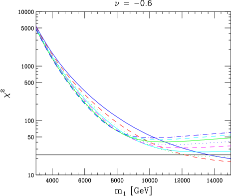
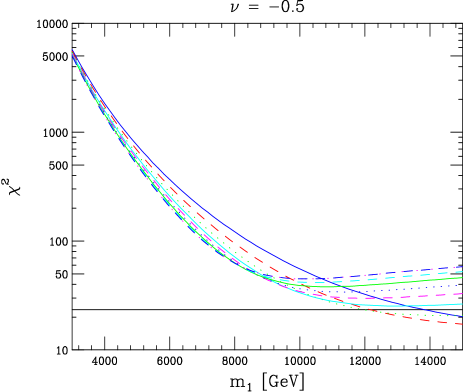
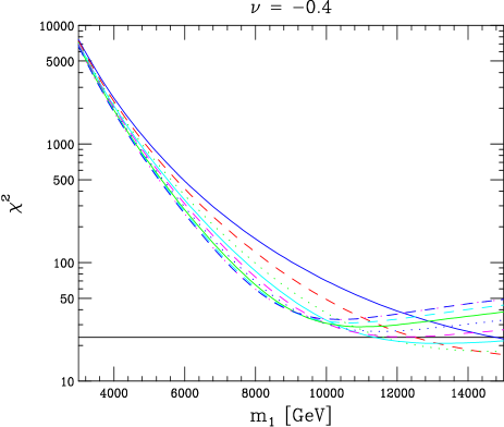
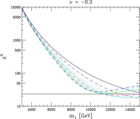
Figure 4: $\chi^{2}$ values obtained in the fit to the EW precision data as a function of $m_{1}$ for four choices of $\nu$, the fermion bulk mass parameter. The solid black line indicates where $\chi^{2}=23.3$, the value at which the 95% CL is reached. The colored curves are the RS model fit results for different Higgs boson masses; from top to bottom, on the left of each plot, the lines indicate $m_{H}=115$, $200$, $300$, …, $1000$ GeV.

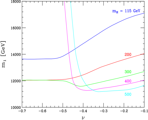
Figure 5: Lowest value of $m_{1}$ that fits the EW data as a function of $\nu$, for five representative choices of $m_{H}$.

5 Searches at the LHC

We now discuss the prospects for detecting the gauge KK states which are consistent with our EW fit at the LHC. The primary discovery mode for new heavy gauge bosons at hadron colliders is high invariant mass Drell-Yan lepton pair production; at the LHC the relevant processes are $pp\rightarrow\gamma^{(1)},Z^{(1)}\rightarrow\mu^{+}\mu^{-}$, $e^{+}e^{-}$. The contributing parton level processes are $q\bar{q}\rightarrow\mu^{+}\mu^{-}$, $e^{+}e^{-}$. We present $d\sigma/dm_{ll}$ for this process (with $m_{ll}$ being the invariant mass of the final state lepton pair) in Fig. 6 for the parameter choices $\nu=-0.6,-0.5,-0.4,-0.3$ and $m_{1}=8,10$ TeV. These values are representative of the allowed region for $\nu$, but the gauge KK masses are lighter than those allowed by the EW fit. If the rates are unobservable at these points in parameter space, then the RS effects are undetectable for all interesting cases. The resonances are wide in this case primarily because of the large couplings of the KK gauge states to top and bottom quarks. With the $100\,{\rm fb}^{-1}$ of integrated luminosity envisioned for the LHC, the KK contributions to Drell-Yan production are indeed invisible. We present the expected number of excess events including both the $\mu^{+}\mu^{-}$ and $e^{+}e^{-}$ channels for this value of integrated luminosity and for the two choices of $\nu$ which produce the largest cross section in Table 3. Here, we have integrated over the invariant mass bins in which there is an excess of events over the SM predictions; this corresponds to the cuts $m_{ll}\mathrel{\mathchoice{\lower 3.01385pt\vbox{\halign{$\matth\displaystyle\hfil#\hfil$\cr>\crcr\sim\crcr}}}{\lower 3.01385pt\vbox{\halign{$\matth\textstyle\hfil#\hfil$\cr>\crcr\sim\crcr}}}{\lower 3.01385pt\vbox{\halign{$\matth\scriptstyle\hfil#\hfil$\cr>\crcr\sim\crcr}}}{\lower 3.01385pt\vbox{\halign{$\matth\scriptscriptstyle\hfil#\hfil$\cr>\crcr\sim\crcr}}}}5$ TeV when $m_{1}=8$ TeV and $\nu=-0.3$, $m_{ll}\mathrel{\mathchoice{\lower 3.01385pt\vbox{\halign{$\matth\displaystyle\hfil#\hfil$\cr>\crcr\sim\crcr}}}{\lower 3.01385pt\vbox{\halign{$\matth\textstyle\hfil#\hfil$\cr>\crcr\sim\crcr}}}{\lower 3.01385pt\vbox{\halign{$\matth\scriptstyle\hfil#\hfil$\cr>\crcr\sim\crcr}}}{\lower 3.01385pt\vbox{\halign{$\matth\scriptscriptstyle\hfil#\hfil$\cr>\crcr\sim\crcr}}}}6.5$ TeV when $m_{1}=8$ TeV and $\nu=-0.4$, $m_{ll}\mathrel{\mathchoice{\lower 3.01385pt\vbox{\halign{$\matth\displaystyle\hfil#\hfil$\cr>\crcr\sim\crcr}}}{\lower 3.01385pt\vbox{\halign{$\matth\textstyle\hfil#\hfil$\cr>\crcr\sim\crcr}}}{\lower 3.01385pt\vbox{\halign{$\matth\scriptstyle\hfil#\hfil$\cr>\crcr\sim\crcr}}}{\lower 3.01385pt\vbox{\halign{$\matth\scriptscriptstyle\hfil#\hfil$\cr>\crcr\sim\crcr}}}}6$ TeV when $m_{1}=10$ TeV and $\nu=-0.3$, and $m_{ll}\mathrel{\mathchoice{\lower 3.01385pt\vbox{\halign{$\matth\displaystyle\hfil#\hfil$\cr>\crcr\sim\crcr}}}{\lower 3.01385pt\vbox{\halign{$\matth\textstyle\hfil#\hfil$\cr>\crcr\sim\crcr}}}{\lower 3.01385pt\vbox{\halign{$\matth\scriptstyle\hfil#\hfil$\cr>\crcr\sim\crcr}}}{\lower 3.01385pt\vbox{\halign{$\matth\scriptscriptstyle\hfil#\hfil$\cr>\crcr\sim\crcr}}}}8$ TeV when $m_{1}=10$ TeV and $\nu=-0.4$. We have not attempted to study the depletion of events at lower $m_{ll}$ because the event rates at the affected invariant masses are too low. Two effects are hindering the detection of the KK contributions: the small couplings of zero mode fermions to KK gauge states for $\nu\leq-0.5$, and the high KK masses which require the parton subprocesses to occur at energies where the quark distribution functions are small. Even with an order of magnitude increase in integrated luminosity, the production of the first gauge KK excitation that is consistent with the EW precision data is unobservable.

	$\nu=-0.4$	$-0.3$
$m_{1}=8$ TeV	$6.4\times 10^{-4}$	$8.8\times 10^{-2}$
$10$ TeV	$4.9\times 10^{-6}$	$3.2\times 10^{-3}$

Table 3: Table of expected Drell-Yan events at the LHC for various parameter choices $L=100\,{\rm fb}^{-1}$. Both the $\mu^{+}\mu^{-}$ and $e^{+}e^{-}$ channels have been included.

Another possible production mechanism for the KK gauge bosons at the LHC is $W^{+}W^{-}$ fusion, $pp\rightarrow WW+2$ jets$\rightarrow V^{(1)}+2$ jets. The relevant triple gauge couplings, $W^{+(0)}W^{-(0)}\gamma^{(1)}$ and $W^{+(0)}W^{-(0)}Z^{(1)}$, are induced by mixing effects. We present the strengths of these vertices normalized to the SM couplings $W^{+}W^{-}\gamma$ and $W^{+}W^{-}Z$ in Fig. 7. Very slight $\nu$ and $m_{H}$ dependences enter these vertices; here we fix $\nu=-0.3$ and $m_{H}=115$ GeV, which maximizes their strength. For $m_{1}\geq 11$ TeV, these couplings are a fraction, $\leq 10^{-3}$, of their SM strengths. This, and the fact that the $W^{+}W^{-}$ fusion process is higher order in the EW coupling constant, render this a poor place in which to search for KK effects.

The only remaining possibility for detecting the KK states at the LHC is via deviations in top and bottom quark production. These processes are dominated at high energies by gluon initiated interactions; however, these do not receive any modifications from gluon KK states since $g^{(0)}g^{(0)}g^{(n)}$ couplings do not exist. We thus only examine top quark production, which receives a larger contribution from quark initiated processes, and where the large couplings of the KK gauge states to third generation quarks enter. The invariant mass distribution is presented in Fig. 8 for $m_{1}=10$ TeV and $\nu=-0.4$. Since the KK couplings to wall fermions do not decrease with KK level, we have checked that the contributions from including multiple states in the KK tower does not significantly enhance the effect. In fact, summing the first five KK contributions slightly decreases the cross section from that where only the first level is included due to the factor of $(-1)^{n}$ that enters the coupling of the $n$th KK level to top quarks. The expected number of excess events at the LHC is $\approx 0.14$, assuming a cut on the invariant mass of the final state top quarks of $m_{tt}\mathrel{\mathchoice{\lower 3.01385pt\vbox{\halign{$\matth\displaystyle\hfil#\hfil$\cr>\crcr\sim\crcr}}}{\lower 3.01385pt\vbox{\halign{$\matth\textstyle\hfil#\hfil$\cr>\crcr\sim\crcr}}}{\lower 3.01385pt\vbox{\halign{$\matth\scriptstyle\hfil#\hfil$\cr>\crcr\sim\crcr}}}{\lower 3.01385pt\vbox{\halign{$\matth\scriptscriptstyle\hfil#\hfil$\cr>\crcr\sim\crcr}}}}3.5$ TeV. As in the previous case of Drell-Yan production, this event rate is undetectable even with an order of magnitude increase in integrated luminosity. The slight depletion of events at lower invariant masses is similarly unobservable. We must therefore conclude that the KK excitations which relax the precision EW upper bound on the Higgs mass are invisible at the LHC.

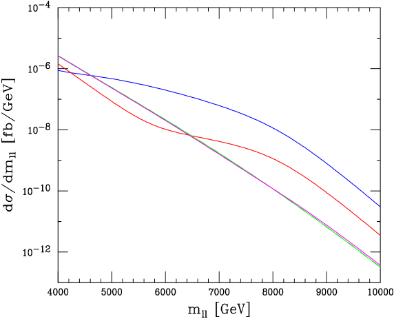
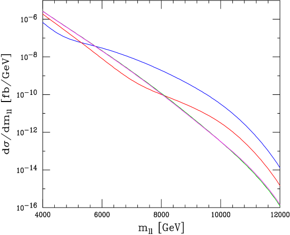
Figure 6: Cross sections for the process $pp\rightarrow\mu^{+}\mu^{-}$ for $m_{1}=8$ TeV (top) and $m_{1}=10$ TeV (bottom) as functions of the final state lepton pair invariant mass. The upper blue curves are for $\nu=-0.3$, the slightly lower red curves represent $\nu=-0.4$, and the three nearly degenerate straight lines correspond to $\nu=-0.5,-0.6$, and the SM. K-factors and a rapidity cut $|\eta|<2.5$ have been included.

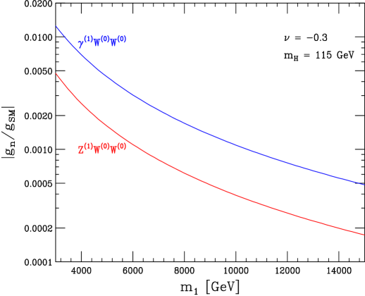
Figure 7: Couplings of $W^{\pm,{(0)}}$ to $\gamma^{(1)}$ and $Z^{(1)}$, normalized to the SM couplings of $W^{\pm}$ to $\gamma$ and $Z$, as functions of $m_{1}$. The parameter values $\nu=-0.3$ and $m_{H}=115$ GeV have been assumed.

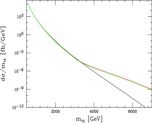
Figure 8: Invariant mass distributions for $pp\rightarrow t\bar{t}$ at the LHC including only the first KK state (top red line) and summing the first five KK gauge bosons (bottom green line), for $m_{1}=10$ TeV. The black line is the SM prediction.

6 Searches at Future TeV-scale Linear Colliders

We examine here whether KK gauge boson exchanges can be observed at a future $e^{+}e^{-}$ collider with $\sqrt{s}=500-1000$ GeV and $L=500-1000\,{\rm fb}^{-1}$. Since the anticipated center-of-mass energies are well below the 11 TeV KK gauge mass defining the lower edge of the allowed range from the EW fit, we study the off-resonance modification of fermion pair production, $e^{+}e^{-}\rightarrow f\bar{f}$. $Z$ pair production receives no KK gauge contribution, while the $\gamma^{(1)}$ and $Z^{(1)}$ exchanges in $e^{+}e^{-}\rightarrow W^{+}W^{-}$ suffer from the weak triple gauge vertices displayed in Fig. 7. We perform a $\chi^{2}$ fit to the total rate, binned angular distribution, and binned ${\cal A}_{LR}$ for fermion pair production to estimate the search reaches possible at TeV-scale linear colliders. We assume an 80% electron beam polarization, a $10^{\circ}$ angular cut, statistical errors and a 0.1% luminosity error. We also use the following reconstructions efficiencies: a 100% $\tau$ efficiency, a 70% $b$ quark efficiency, a 50% $t$ quark efficiency, and a 40% $c$ quark efficiency. The $\chi^{2}$ values obtained in this analysis are shown in Fig. 9 for several choices of $\sqrt{s}$ and $L$.

We see from Fig. 9 that the effects of KK exchange exceed the 95% CL exclusion limit for all $\nu$ values in the allowed region and for $m_{1}\leq 15$ TeV; the modifications when $\nu\geq-0.4$ reach the $5\sigma$ discovery limit. The parameter space $\nu\leq-0.5$ and $m_{1}>15$ TeV, part of which provides a good fit to the EW precision data, falls below the exclusion limit. It is possible that this difficulty can be alleviated with the inclusion of more observables. We note that a small hierarchy between the EW scale and $\Lambda_{\pi}$ begins to develop in this region, and it is consequently not as favored as the $m_{1}\leq 15$ TeV range. We note that the ordering of the $\nu=-0.6$ and $-0.5$ curves in the lower figure of Fig. 9 is correct.

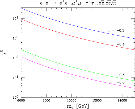
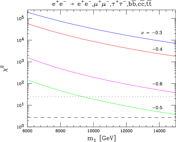
Figure 9: $\chi^{2}$ values obtained by fitting the RS model predictions for fermion pair production to the SM for $\nu=-0.6,-0.5,-0.4,-0.3$, as functions of $m_{1}$. The upper figure assumes $\sqrt{s}=500$ GeV and $L=500\,{\rm fb}^{-1}$, while the lower assumes $\sqrt{s}=1000$ GeV and $L=1000\,{\rm fb}^{-1}$. The dashed line indicates the $\chi^{2}$ necessary for exclusion of the model at the 95% CL, and the dotted line illustrates the $\chi^{2}$ required for a $5\sigma$ discovery. The polarizations and reconstruction efficiencies assumed are presented in the text.

We now subject this model to future high precision tests. Planned $e^{+}e^{-}$ colliders are designed for operation on the $Z$-pole for a period sufficient to collect $10^{9}$ $Z$ events. This program, known as GigaZ, will reduce the error in ${\rm sin}^{2}\theta_{eff}$ to the $10^{-5}$ level and the error in $R_{b}$ by a factor of 5 [23]. A phase of operation on the $W^{\pm}$ pair production threshold is also planned, which will reduce the error in the measurement of $M_{W}$ to 6 MeV. We now return to our analysis of EW precision data and study the effects of this error reduction, keeping the central values for the observables unchanged from the present and focusing on ${\rm sin}^{2}\theta_{eff}$, $M_{W}$, and $R_{b}$. Figures 10 and 11 display our results in the ${\rm sin}^{2}\theta_{eff}$ versus $M_{W}$ plane and the ${\rm sin}^{2}\theta_{eff}$ versus $R_{b}$ plane for $\nu=-0.5$ and $-0.4$. These figures show the current and expected experimental precisions, SM predictions, and RS model results for several different Higgs masses and $m_{1}$ choices.

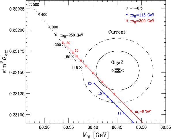
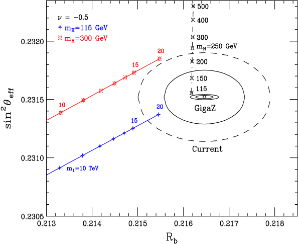
Figure 10: The planes ${\rm sin}^{2}\theta_{eff}$ versus $M_{W}$ (top) and ${\rm sin}^{2}\theta_{eff}$ versus $R_{b}$ (bottom) showing current and future sensitivities, SM predictions, and RS model predictions. The diamonds show the current measured values of the observables. The large solid and dashed ellipses represent respectively the 68% and 95% CL regions from current sensitivities, while the smaller solid ellipses anticipate the same after operation of GigaZ. The black dashdot lines show the SM predictions for different Higgs boson masses as labeled, while the solid colored lines show the RS model results for varying $m_{1}$ for two Higgs masses satisfying the current EW constraints.

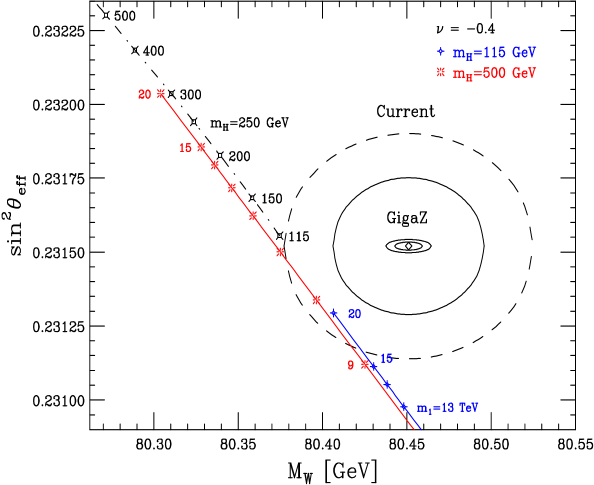
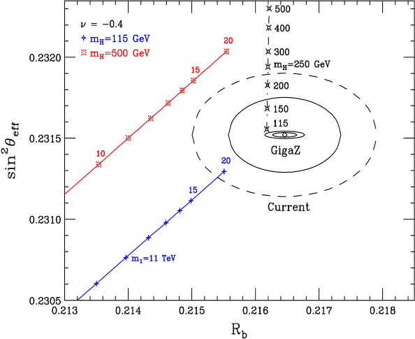
Figure 11: Same as the previous figure for $\nu=-0.4$, and different $m_{H}$ choices.

It is difficult to predict what the status of fits to the EW precision data will be after the GigaZ program concludes, as a small shift in the experimental central values assisted by the small anticipated errors can drastically alter the current situation. If the central values remain unchanged, it is clear from these figures that the improved precision in the measurement of $R_{b}$ will disfavor the heavier Higgs solutions, and require a large value of $m_{1}$, which reintroduces a hierarchy between $\Lambda_{\pi}$ and the EW scale. However, the RS predictions for ${\rm sin}^{2}\theta_{eff}$ and $M_{W}$ match experiment better than the SM results and can accommodate a heavy Higgs, and the global fit to the EW observables may prefer this solution. Whatever scenario is realized, it is certainly true that the entire parameter space, including the region inaccessible in off-resonance fermion pair production, can be probed at GigaZ.

7 Constraints from FCNCs

The placement of fermions in different locations in extra dimensions, on the TeV brane or in the bulk, leads to potentially dangerous FCNC since the Glashow-Weinberg-Paschos conditions [24, 25] for the natural absence of FCNC are no longer satisfied. These conditions are violated automatically whenever fermions of different generations are treated asymmetrically by some form of new physics and mixing occurs between the relevant states. Within the RS scenario that we have constructed, these FCNC can arise from a number of potential sources, not all of which present the same level of danger. A detailed analysis of FCNC effects is certainly beyond the scope of this paper and requires a specific flavor model as input; we simply outline the potential sources of FCNC and provide a few estimates of their size.

The most obvious sources of FCNC are from the exchanges of gauge bosons. The states in the gauge KK towers can feel the different fermion generation localities, and through intergenerational mixing can then induce FCNC. Furthermore, the couplings of the wall fields to the KK gauge states are enhanced by a factor of $\approx\sqrt{2\pi kr_{c}}$. Since zero mode KK gauge states in the limit of vanishing mixing are constrained by construction to have the same couplings to fermions as do the SM gauge bosons, such fields can only induce FCNC through the small admixture of KK weak eigenstates introduced by mixing. These effects are suppressed by small mixing angles, and are not as important as those arising from the KK towers themselves. We therefore expect that the KK gauge state contributions represent the greatest source of potentially dangerous FCNC.

Graviton KK towers can also probe the different locations of the SM fermion generations and induce FCNC-like couplings. However, in this case the potentially dangerous contributions are much smaller since ($i$) graviton-induced FCNC take the form of dimension-8 operators, in contrast to the dimension-6 KK gauge contributions, and lead to amplitudes which are suppressed by factors of order $m_{K,D,B}^{2}/\Lambda_{\pi}^{2}$. This is an enormous degree of suppression since we have shown that $\Lambda_{\pi}\mathrel{\mathchoice{\lower 3.01385pt\vbox{\halign{$\matth\displaystyle\hfil#\hfil$\cr>\crcr\sim\crcr}}}{\lower 3.01385pt\vbox{\halign{$\matth\textstyle\hfil#\hfil$\cr>\crcr\sim\crcr}}}{\lower 3.01385pt\vbox{\halign{$\matth\scriptstyle\hfil#\hfil$\cr>\crcr\sim\crcr}}}{\lower 3.01385pt\vbox{\halign{$\matth\scriptscriptstyle\hfil#\hfil$\cr>\crcr\sim\crcr}}}}10$ TeV in the scenario presently under consideration. ($ii$) Unlike KK gauge fields, the graviton KK couplings to wall fields are not enhanced by the factor $\sqrt{2\pi kr_{c}}$.

How large are the KK gauge tower contributions? The answer depends upon which gauge boson we are examining. We neglect in this analysis the small mixing between the first and second generation fermions and their KK towers. Let $g_{L,R}^{a}$ represent the couplings of a particular fermion with electric charge $Q$ to one of the neutral SM gauge bosons labeled by the index $a$. We write the fermion couplings to KK gauge states as $g_{L,R}^{a}c^{n}(\nu_{i})$, where $\nu_{i}$ is the $i$th generation bulk mass parameter and $n$ labels the gauge KK tower level. Note that the functions $c^{n}$ in the present model are independent of chirality and the gauge boson under consideration. The fact that the $c^{n}(\nu_{i})$ are different for each $i$ generates the FCNC terms when we transform to the mass eigenstate basis. Let $U_{L,R}$ represent the matrices performing the bi-unitary transformation required to diagonalize the appropriate fermion mass matrix. The off-diagonal couplings in the mass eigenstate basis are then given by

$$(Q^{n}_{L,R})^{a}_{ij}=g_{L,R}^{a}\sum_{k}(U_{ik})_{L,R}c^{n}(\nu_{k})(U^{\dagger}_{kj})_{L,R}\,.$$ (53)

For the specific model discussed in the previous sections we have $c^{n}(\nu_{1})=c^{n}(\nu_{2})\neq c^{n}(\nu_{3})$, and we use the unitarity of the $U$’s to rewrite these couplings as

$$(Q^{n}_{L,R})^{a}_{ij}=g_{L,R}^{a}[c^{n}(\nu_{3})-c^{n}(\nu_{1})](U_{i3}U^{\dagger}_{3j})_{L,R}\,.$$ (54)

With the third generation on the wall and the first and second in the bulk in the region $-0.6\leq\nu_{1}\leq-0.3$, it is clear that $|c^{n}(\nu_{3})-c^{n}(\nu_{1})|\simeq\sqrt{2\pi kr_{c}}$ for all $n$; at worst, the size of the off-diagonal couplings in our model is given by

$$(Q^{n}_{L,R})^{a}_{ij}=\sqrt{2\pi kr_{c}}\,g_{L,R}^{a}(U_{i3}U^{\dagger}_{3j})_{L,R}\,,$$ (55)

which is independent of $n$. The $U_{ij}$ arise from some complete theory of flavor that must reproduce the experimentally measured CKM matrix $V_{ij}$. We therefore expect $U_{ij}\simeq V_{ij}$ and ee adopt this approximation in our estimates below.

The most stringent constraints on FCNC arise from low energy processes such as meson-antimeson mixing and rare decays [26]; we present here our estimate for $K-\bar{K}$ mixing. The above interaction generates a coupling which can be symbolically written as

$${\cal L}=2\pi kr_{c}\sum_{a}\sum_{n}(J^{a}_{L}+J^{a}_{R})^{2}/m_{n}^{2}\,,$$ (56)

where $J^{a}_{L,R}=g_{L,r}^{a}V_{i3}V^{\dagger}_{3j}\bar{f}_{i}\gamma_{\mu}P_{L,R}f_{j}$, $m_{n}$ is the mass of the $n$th KK gauge state, and we have summed all KK contributions. Recalling the lore that we can accurately approximate the matrix element of the two currents in the vacuum insertion approximation, we see that the KK gluon towers do not contribute. This is due to the fact that these states only couple to currents with non-zero color while both the meson and the vacuum are color singlets. Thus we need to consider only the $Z$ and $\gamma$ tower exchanges. Using $\sum_{n}m_{n}^{-2}\simeq 1.5m_{1}^{-2}$ [4], $V_{13}V^{\dagger}_{32}\simeq A^{2}(1-\rho)^{2}\lambda^{5}$ in the Wolfenstein parameterization and

$$<K|J_{L}J_{R}|\bar{K}>=\Omega_{K}<K|J_{L}J_{L}|\bar{K}>=\Omega_{K}<K|J_{R}J_{R}|\bar{K}>\,,$$ (57)

with $\Omega_{K}\simeq 7$ [27] for the current-current matrix element, we arrive at

$${{\Delta m_{KK}^{RS}}\over{\Delta m_{KK}^{SM}}}\simeq 0.0098[1+0.73\Omega_{K}]\left(11TeV\over{m_{1}}\right)^{2}\simeq 0.06\,,$$ (58)

which is within the uncertainty of the SM result [28]. From this estimate we see that, at least for the $K-\bar{K}$ system, the RS FCNC contributions are rather small. We have also studied $B-\bar{B}$ mixing and obtain similar results.

Once a realistic theory of flavor within this RS model context is constructed, we can perform a more detailed and quantitative analysis of the potential impact of FCNC. It will be interesting to examine if existing bounds can provide further constraints on the RS model parameters within such a framework.

8 Discussions and Conclusions

In this paper we have re-examined the placement of SM fermions in the full 5-dimensional bulk of the Randall-Sundrum spacetime. We have found that mixing between the top quark zero mode and its KK tower, induced by the large top quark mass, yields shifts in the $\rho$ parameter that are inconsistent with current measurements. To obviate these bounds we must take the fundamental RS scale $\Lambda_{\pi}\mathrel{\mathchoice{\lower 3.01385pt\vbox{\halign{$\matth\displaystyle\hfil#\hfil$\cr>\crcr\sim\crcr}}}{\lower 3.01385pt\vbox{\halign{$\matth\textstyle\hfil#\hfil$\cr>\crcr\sim\crcr}}}{\lower 3.01385pt\vbox{\halign{$\matth\scriptstyle\hfil#\hfil$\cr>\crcr\sim\crcr}}}{\lower 3.01385pt\vbox{\halign{$\matth\scriptscriptstyle\hfil#\hfil$\cr>\crcr\sim\crcr}}}}100$ TeV, reintroducing the hierarchy between the Planck and EW scales and thus destroying the original motivation for the RS model. We instead proposed a mixed scenario which localizes the third generation of quarks, and presumably leptons, on the TeV-brane and allows the lighter two generations to propagate in the RS bulk. For values of the bulk mass parameter in the region $-0.55\mathrel{\mathchoice{\lower 3.01385pt\vbox{\halign{$\matth\displaystyle\hfil#\hfil$\cr<\crcr\sim\crcr}}}{\lower 3.01385pt\vbox{\halign{$\matth\textstyle\hfil#\hfil$\cr<\crcr\sim\crcr}}}{\lower 3.01385pt\vbox{\halign{$\matth\scriptstyle\hfil#\hfil$\cr<\crcr\sim\crcr}}}{\lower 3.01385pt\vbox{\halign{$\matth\scriptscriptstyle\hfil#\hfil$\cr<\crcr\sim\crcr}}}}\nu\mathrel{\mathchoice{\lower 3.01385pt\vbox{\halign{$\matth\displaystyle\hfil#\hfil$\cr<\crcr\sim\crcr}}}{\lower 3.01385pt\vbox{\halign{$\matth\textstyle\hfil#\hfil$\cr<\crcr\sim\crcr}}}{\lower 3.01385pt\vbox{\halign{$\matth\scriptstyle\hfil#\hfil$\cr<\crcr\sim\crcr}}}{\lower 3.01385pt\vbox{\halign{$\matth\scriptscriptstyle\hfil#\hfil$\cr<\crcr\sim\crcr}}}}-0.35$, the same values allowed by both contact interaction searches and $\rho$ parameter constraints arising from the first two generations, the fermions mass hierarchies $m_{c}/m_{t}$ and $m_{s}/m_{b}$ are naturally reproduced.

We next explored the consequences of this proposal for current precision EW measurements. We studied modifications of the electroweak observables caused by both mixing of the SM gauge bosons with their corresponding KK towers and the exchanges of higher KK states; we found that with KK masses $m_{1}\approx 11$ TeV and bulk mass parameters $\nu\approx-0.5,-0.4$ a Higgs boson with mass $m_{H}\mathrel{\mathchoice{\lower 3.01385pt\vbox{\halign{$\matth\displaystyle\hfil#\hfil$\cr<\crcr\sim\crcr}}}{\lower 3.01385pt\vbox{\halign{$\matth\textstyle\hfil#\hfil$\cr<\crcr\sim\crcr}}}{\lower 3.01385pt\vbox{\halign{$\matth\scriptstyle\hfil#\hfil$\cr<\crcr\sim\crcr}}}{\lower 3.01385pt\vbox{\halign{$\matth\scriptscriptstyle\hfil#\hfil$\cr<\crcr\sim\crcr}}}}500$ GeV can provide a good fit to the precision electroweak data. An analysis of the fit showed that the large couplings between the zero mode bottom quark and KK gauge bosons induced large shifts in $R_{b}$ that prevented a heavier Higgs from being consistent with the precision data.

We then examined the signatures of this scenario at future high energy colliders. We found that the parameter region consistent with the precision electroweak data does not lead to any new physics signatures at the LHC; the expected event excess in both Drell-Yan and gauge boson fusion processes are statistically insignificant with the envisioned integrated luminosities, and the predicted modification of the $t\bar{t}$ production cross section is similarly unobservably small. The only new physics that the LHC would possibly observe is a Higgs boson apparently heavier than that allowed by the SM electroweak fits. By contrast, the parameter range $m_{1}\mathrel{\mathchoice{\lower 3.01385pt\vbox{\halign{$\matth\displaystyle\hfil#\hfil$\cr<\crcr\sim\crcr}}}{\lower 3.01385pt\vbox{\halign{$\matth\textstyle\hfil#\hfil$\cr<\crcr\sim\crcr}}}{\lower 3.01385pt\vbox{\halign{$\matth\scriptstyle\hfil#\hfil$\cr<\crcr\sim\crcr}}}{\lower 3.01385pt\vbox{\halign{$\matth\scriptscriptstyle\hfil#\hfil$\cr<\crcr\sim\crcr}}}}15$ TeV and $\nu\mathrel{\mathchoice{\lower 3.01385pt\vbox{\halign{$\matth\displaystyle\hfil#\hfil$\cr<\crcr\sim\crcr}}}{\lower 3.01385pt\vbox{\halign{$\matth\textstyle\hfil#\hfil$\cr<\crcr\sim\crcr}}}{\lower 3.01385pt\vbox{\halign{$\matth\scriptstyle\hfil#\hfil$\cr<\crcr\sim\crcr}}}{\lower 3.01385pt\vbox{\halign{$\matth\scriptscriptstyle\hfil#\hfil$\cr<\crcr\sim\crcr}}}}-0.3$ can be probed in fermion pair production processes at a future $e^{+}e^{-}$ collider with center-of-mass energy of $500-1000$ GeV, while the region $m_{1}\mathrel{\mathchoice{\lower 3.01385pt\vbox{\halign{$\matth\displaystyle\hfil#\hfil$\cr<\crcr\sim\crcr}}}{\lower 3.01385pt\vbox{\halign{$\matth\textstyle\hfil#\hfil$\cr<\crcr\sim\crcr}}}{\lower 3.01385pt\vbox{\halign{$\matth\scriptstyle\hfil#\hfil$\cr<\crcr\sim\crcr}}}{\lower 3.01385pt\vbox{\halign{$\matth\scriptscriptstyle\hfil#\hfil$\cr<\crcr\sim\crcr}}}}25-30$ TeV and $\nu\mathrel{\mathchoice{\lower 3.01385pt\vbox{\halign{$\matth\displaystyle\hfil#\hfil$\cr<\crcr\sim\crcr}}}{\lower 3.01385pt\vbox{\halign{$\matth\textstyle\hfil#\hfil$\cr<\crcr\sim\crcr}}}{\lower 3.01385pt\vbox{\halign{$\matth\scriptstyle\hfil#\hfil$\cr<\crcr\sim\crcr}}}{\lower 3.01385pt\vbox{\halign{$\matth\scriptscriptstyle\hfil#\hfil$\cr<\crcr\sim\crcr}}}}-0.3$ is testable at GigaZ. For larger KK first excitation masses, we reintroduce the hierarchy between $\Lambda_{\pi}$ and the electroweak scale.

Finally, we considered the possible constraints on this scenario arising from low energy FCNC. The asymmetric treatment of the three fermion generations allows KK $Z$-boson exchanges to mediate FCNC interactions. We estimated the contributions of such effects to meson-antimeson mixing, and found that their size is within the theoretical errors inherent to meson mixing. However, a detailed analysis of FCNC effects requires a full model of flavor, which we have not constructed.

In summary, we have found that the experimental restrictions on placing SM matter in the RS bulk lead naturally to a very interesting region of parameter space. This parameter region provides a geometrical origin for the fermion Yukawa hierarchies, and allows a heavy Higgs boson to be consistent with precision measurements while remaining otherwise invisible at the LHC. We believe that such features render this model worthy of further study.

Acknowledgements

F.P. would like to thank K. Melnikov for discussions. The work of F.P. was supported in part by the National Science Foundation Graduate Research Program.

References

- [1] L. Randall and R. Sundrum, Phys. Rev. Lett. 83, 3370 (1999) [arXiv:hep-ph/9905221]; Phys. Rev. Lett. 83, 4690 (1999) [arXiv:hep-th/9906064].
- [2] W. D. Goldberger and M. B. Wise, Phys. Rev. Lett. 83, 4922 (1999) [arXiv:hep-ph/9907447]; W. D. Goldberger and M. B. Wise, Phys. Lett. B 475, 275 (2000) [arXiv:hep-ph/9911457]; C. Csaki, M. Graesser, L. Randall and J. Terning, Phys. Rev. D 62, 045015 (2000) [arXiv:hep-ph/9911406]; C. Csaki, M. L. Graesser and G. D. Kribs, Phys. Rev. D 63, 065002 (2001) [arXiv:hep-th/0008151]; T. Tanaka and X. Montes, Nucl. Phys. B 582, 259 (2000) [arXiv:hep-th/0001092].
- [3] H. Davoudiasl, J. L. Hewett and T. G. Rizzo, Phys. Rev. Lett. 84, 2080 (2000) [arXiv:hep-ph/9909255].
- [4] H. Davoudiasl, J. L. Hewett and T. G. Rizzo, Phys. Lett. B 473, 43 (2000) [arXiv:hep-ph/9911262].
- [5] A. Pomarol, Phys. Lett. B 486, 153 (2000) [arXiv:hep-ph/9911294].
- [6] C. Csaki, J. Erlich and J. Terning, arXiv:hep-ph/0203034; S. J. Huber, C. A. Lee and Q. Shafi, Phys. Lett. B 531, 112 (2002) [arXiv:hep-ph/0111465].
- [7] Y. Grossman and M. Neubert, Phys. Lett. B 474, 361 (2000) [arXiv:hep-ph/9912408].
- [8] S. Chang, J. Hisano, H. Nakano, N. Okada and M. Yamaguchi, Phys. Rev. D 62, 084025 (2000) [arXiv:hep-ph/9912498]; R. Kitano, Phys. Lett. B 481, 39 (2000) [arXiv:hep-ph/0002279]; T. Gherghetta and A. Pomarol, Nucl. Phys. B 586, 141 (2000) [arXiv:hep-ph/0003129]; S. J. Huber and Q. Shafi, Phys. Rev. D 63, 045010 (2001) [arXiv:hep-ph/0005286]; Phys. Lett. B 498, 256 (2001) [arXiv:hep-ph/0010195]; Phys. Lett. B 512, 365 (2001) [arXiv:hep-ph/0104293].
- [9] H. Davoudiasl, J. L. Hewett and T. G. Rizzo, Phys. Rev. D 63, 075004 (2001) [arXiv:hep-ph/0006041].
- [10] H. Davoudiasl, J. L. Hewett and T. G. Rizzo, Phys. Lett. B 493, 135 (2000) [arXiv:hep-ph/0006097].
- [11] M. E. Peskin and T. Takeuchi, Phys. Rev. Lett. 65, 964 (1990).
- [12] For a recent summary of experimental measurements, see D. Charlton, arXiv:hep-ex/0110086. For the latest results from NuTeV, see G. P. Zeller et al. [NuTeV Collaboration], arXiv:hep-ex/0110059.
- [13] F. del Aguila and J. Santiago, Phys. Lett. B 493, 175 (2000) [arXiv:hep-ph/0008143].
- [14] F. del Aguila and J. Santiago, arXiv:hep-ph/0011143.
- [15] M. J. Veltman, Nucl. Phys. B 123, 89, 1977.
- [16] P. Langacker, in Proc. of the APS/DPF/DPB Summer Study on the Future of Particle Physics (Snowmass 2001) ed. R. Davidson and C. Quigg, arXiv:hep-ph/0110129.
- [17] For a comparison of other scenarios which relax the constraint on the Higgs boson mass obtained by the standard EW fit, see, M. E. Peskin and J. D. Wells, Phys. Rev. D 64, 093003 (2001) [arXiv:hep-ph/0101342].
- [18] G. Altarelli, R. Kleiss and C. Verzegnassi, Geneva, Switzerland: CERN (1989) 453 p. CERN Geneva - CERN 89-08 (89,rec.Dec.) 453 p.
- [19] M. Masip and A. Pomarol, Phys. Rev. D 60, 096005 (1999) [arXiv:hep-ph/9902467].
- [20] T. G. Rizzo and J. D. Wells, Phys. Rev. D 61, 016007 (2000) [arXiv:hep-ph/9906234].
- [21] D. Y. Bardin, P. Christova, M. Jack, L. Kalinovskaya, A. Olchevski, S. Riemann and T. Riemann, Comput. Phys. Commun. 133, 229 (2001) [arXiv:hep-ph/9908433].
- [22] The LEP Electroweak Working Group (The LEP and SLD Collaborations), LEPEWWG/2001-02, December 2001.
- [23] J. A. Aguilar-Saavedra et al. [ECFA/DESY LC Physics Working Group Collaboration], arXiv:hep-ph/0106315.
- [24] S. L. Glashow and S. Weinberg, Phys. Rev. D 15, 1958 (1977).
- [25] E. A. Paschos, Phys. Rev. D 15, 1966 (1977).
- [26] D. E. Groom et al. [Particle Data Group Collaboration], Eur. Phys. J. C 15, 1 (2000).
- [27] See, for example, G. Beall, M. Bander and A. Soni, Phys. Rev. Lett. 48, 848 (1982).
- [28] For a review of the SM contributions to mixing, see A. J. Buras, arXiv:hep-ph/0101336.