FERMI–PUB–02/045-T

BUHEP-01-09

March, 2003

Strong Dynamics and Electroweak
Symmetry Breaking

Christopher T. Hill¹
and

Elizabeth H. Simmons^2,3

¹Fermi National Accelerator Laboratory
P.O. Box 500, Batavia, IL, 60510

² Dept. of Physics, Boston University
590 Commonwealth Avenue, Boston, MA, 02215

³ Radcliffe Institute for Advanced Study and
Department of Physics, Harvard University
Cambridge, MA, 02138

Abstract

The breaking of electroweak symmetry, and origin of the associated “weak scale,” $v_{weak}=1/\sqrt{2\sqrt{2}G_{F}}=175$ GeV, may be due to a new strong interaction. Theoretical developments over the past decade have led to viable models and mechanisms that are consistent with current experimental data. Many of these schemes feature a privileged role for the top quark, and third generation, and are natural in the context of theories of extra space dimensions at the weak scale. We review various models and their phenomenological implications which will be subject to definitive tests in future collider runs at the Tevatron, and the LHC, and future linear $e^{+}e^{-}$ colliders, as well as sensitive studies of rare processes.

1 Introduction

1.1 Lessons from QCD

The early days of accelerator-based particle physics were largely explorations of the strong interaction scale, associated roughly with the proton mass, of order 1 GeV. Key elements were the elaboration of the hadron spectroscopy; the measurements of cross-sections; the elucidation of spontaneously broken chiral symmetry, with the pion as a Nambu-Goldstone phenomenon [1, 2, 3]; the evolution of the flavor symmetry $SU(3)$ and the quark model [4, 5, 6]; the discovery of scaling behavior in electroproduction; [7, 8, 9]; and the observation of quarks and gluons as partons. Eventually, this work culminated in Quantum Chromodynamics (QCD): a description of the strong scale based upon the elegant symmetry principle of local gauge invariance, and the discovery of the Yang-Mills gauge group $SU(3)$ of color [10, 11]. Today we recognize that the strong scale is a well-defined quantity, $\Lambda_{QCD}\sim 100$ MeV, the infrared scale at which the perturbatively defined running coupling constant of QCD blows up, and we are beginning to understand how to perform detailed nonperturbative numerical computations of the associated phenomena.

There are several lessons in the discovery of QCD which illuminate our present perspective on nature. First, it took many years to get from the proton, neutron, and pions, originally thought to be elementary systems, to the underlying theory of QCD. From the perspective of a physicist of the 1930’s, knowing only the lowest-lying states, or one of the 1950’s seeing the unfolding of the resonance spectroscopy and new quantum numbers, such as strangeness, it would have seemed astonishing that those disparate elements came from a single underlying Yang-Mills gauge theory [12]. Second, the process of solving the problem of the strong interactions involved a far-ranging circumnavigation of all of the ideas that we use in theoretical physics today. For example, the elaboration of the resonance spectrum and Regge behavior of QCD led to the discovery of string theory! QCD embodies a rich list of phenomena, including confinement, perturbative asymptotic freedom [13, 14], topological fluctuations, and, perhaps most relevant for our present purposes, a BCS-like [15, 16] mechanism leading to chiral symmetry breaking [1, 2, 3]. Finally, the strong interactions are readily visible in nature for what might be termed “contingent” reasons: the nucleon is stable, and atomic nuclei are abundant. If a process like $p\rightarrow e^{+}+\gamma$ occured with a large rate, so that protons were short-lived, then the strong interactions would be essentially decoupled from low energy physics, for $\sqrt{s}<2m_{\pi}$. A new strong dynamics, if it exists, presumably does not have an analogous stable sector (else we would have seen it), and this dynamics must be largely decoupled below threshold.

QCD provides direct guidance for this review because of the light it may shed on the scale of electroweak symmetry breaking (EWSB). The origin of the scale $\Lambda_{QCD}$, and the “hierarchy” between the strong and gravitational scales is, in principle, understood within QCD in a remarkable and compelling way. If a perturbative input for $\alpha_{s}$ is specified at some high energy scale, e.g., the Planck scale, then the logarithmic renormalization group running of $\alpha_{s}$ naturally produces a strong-interaction scale $\Lambda_{QCD}$ which lies far below $M_{Planck}$. The value of scale $\Lambda_{QCD}$ does not derive directly from the Planck scale, e.g. through multiplication by some ratio of coupling constants. Rather $\Lambda_{QCD}$ arises naturally and elegantly from quantum mechanics itself, through dimensional transmutation [17]. Hence, QCD produces the large hierarchy of scales without fine-tuning. The philosophy underlying theories of dynamical EWSB is that the “weak scale” has a similar dynamical and natural origin.

1.2 The Weak Scale

We have mentioned two of the fundamental mass scales in nature, the strong-interaction scale $\Lambda_{QCD}$ and the scale of gravity, $M_{Planck}=(\sqrt{G_{N}})^{-1}\approx 10^{19}$ GeV. The mass scale, which will figure most directly in our discussion, is the scale of weak physics, $v_{weak}=(\sqrt{2\sqrt{2}G_{F}})^{-1}=175$ GeV. The weak scale first entered physics, approximately 70 years ago, when Enrico Fermi constructed the current-current interaction description of $\beta$-decay and introduced the constant, $G_{F}$, into modern physics [18]. The Standard Model [19, 20, 21] identifies $v_{weak}$ with the vacuum expectation value (VEV) of a fundamental, isodoublet, “Higgs” scalar field. Both the gravitational and weak scales are associated with valid low energy effective theories. In the case of $M_{Planck}$ we have classical General Relativity; In the case of $v_{weak}$ we have the Standard Model.

The Standard Model is predictive and enjoys spectacular success in almost all applications to the analysis of existing experimental data. This hinges upon its renormalizability: it is a valid quantum theory. Now that current experiments are sensitive to electroweak loop effects, these two aspects have become closely entwined. In almost all channels, experiment continues simply to confirm the Standard Model’s predictions; those processes which are sensitive to loop contributions are starting to constrain the mass of the Higgs Boson. Combining all experimental data sensitive to electroweak loop corrections yields an upper bound on the Standard Model Higgs boson’s mass of order $200$ GeV [22].

Beyond this fact, however, we know nothing in detail about the Higgs boson, or whether or not it actually exists as a fundamental particle in nature. If new dynamics were assumed to be present at the TeV scale, the Higgs boson could be a bound state and the upper bound on the composite Higgs mass would rise to $\sim$ 1 TeV [24]. Certain models we will describe in this review, such as the Top Quark Seesaw scheme, predict a composite Higgs boson with a mass $m_{H}\sim 1$ TeV and are otherwise in complete agreement with electroweak constraints (see Section 4).

In considering the Higgs sector, the foremost question is that of motive: “why should nature provide a unique elementary particle simply for the purpose of breaking a symmetry?” Other issues involve naturalness, i.e., the degree of fine-tuning required to provide the scale of the mass of the putative Higgs boson [25, 26, 27]. Certainly, when compared to the completely natural origin of $\Lambda_{QCD}$ relative to $M_{Planck}$, the origin of a Higgs boson mass, $m_{H}\sim 200$ GeV in the Standard Model is a complete mystery. These questions hint at the need for a more general mechanism or some enveloping symmetries that do the equivalent job of, or provide a rationalization for, the Higgs Boson. Therefore, it is fair to say that the true mechanism of EWSB in nature is unknown.

The paradigm we will explore in the present review is that the EWSB physics, in analogy to the strong interactions of QCD, arises from novel strong dynamics. We emphasize at the outset that new strong dynamics (NSD) is incompatable with a completely perturbative view of physics near the electroweak scale – but does not exclude the possibility of a low-scale Supersymmetry (SUSY). For the most part in this review, our discussion will focus on the nature and implications of the new strong dynamics itself, and not on the additional possible presence of SUSY.

In focusing this review in this direction, we should consider what we hope to learn by looking beyond the more popular supersymmetric theories. Certainly, SUSY is an elegant extension of the Lorentz group that fits naturally into string theory, our best candidate for a quantum theory of gravity. SUSY, moreover, gives us an intriguing raison d’etre for the existence of fundamental scalar particles: If we look at the fermionic content of a model, such as the Minimal Supersymmetric Standard Model (MSSM) we see that Higgs bosons can be viewed as superpartners of new vector-like leptons (i.e., a pair of left-handed leptonic isodoublets, one with $Y=1$ and the other with $Y=-1$ in the MSSM). As additional rewards we find that: (i) the hierarchy, while not explained, is protected by the chiral symmetries of the fermions; (ii) the resulting theory can be weakly coupled and amenable to perturbative studies; and (iii) there is reasonably precise unification of the gauge coupling constants.

On the other hand, SUSY offers fairly limited insight into why there occurs EWSB, since the Higgs sector is essentially added by hand, just as the original Higgs boson was added to the Standard Model, to accomodate the phenomenon. The significance of the successful unification of the gauge coupling constants [28, 29, 30], which is certainly one of the more tantalizing aspects of the MSSM, is nevertheless inconclusive because the unification condition that obtains in nature remains unknown. For example, higher dimension operators associated with the Planck or GUT scales can modify the naive unification condition, thus permitting unification in models that might otherwise be rejected [31, 32]. Moreover, new Strong Dynamical Models (NSD’s) of EWSB can in principle unify. However, because the primary dynamical issues in models of new strong dynamics arise at the weak scale and because complete NSD models are few in number, unification of NSD models has not been developed very far.

We believe that the central problem facing particle physics today is to explain the origin of the electroweak mass scale, or equivalently, EWSB: What causes the scale $v_{weak}\propto(G_{F})^{-1/2}$ in nature? Theories of new strong dynamics offer new insights into possible mechanisms of electroweak symmetry breaking. We recall that before QCD was understood to be a local gauge theory with its intrinsic rich dynamics, speculation about what lay beyond the strong interaction scale was systematically flawed. Thus, while many of the fundamental symmetries controlling the known forces in nature are understood, speculation as to what lies on energy scales well above $v_{weak}$ should be viewed as tentative. Let us therefore focus on physics at the weak scale.

We will begin by providing an introductory tutorial survey of the elementary physical ingredients of dynamical symmetry breaking. In Section 1.3, we will consider a sequence of “five easy pieces,” or illustrative models which successively incorporate the key elements of the electroweak Standard Model. This is complemented by a discussion of the full Standard Model, including oblique radiative corrections, in 1.4, 3.2, and Appendix A, and by a discussion of a toy model of strong dynamics, the Nambu–Jona-Lasinio model, in Appendix B. Issues related to naturalness in the QCD and electroweak sectors of the Standard Model are discussed in Section 1.4. These are intended to provide newcomers or non-specialists with the collected ideas and a common language to make the rest of the review accessible. The arrangement of our discussion of modern theories and phenomenology of dynamical EWSB is given in Section 1.5.

A reader who may wish to “cut to the chase” is advised to skip directly to Section 1.5.

1.3 Superconductors, Chiral Symmetries, and Nambu-Goldstone Bosons

A particle physicist’s definition of an ordinary electromagnetic superconductor is a “vacuum” or groundstate in which the photon becomes massive. For example, when a block of lead (Pb) is cooled to $3^{o}K$ in the laboratory, photons impinging on the material acquire a mass of about $1$ eV, and the associated phenomena of superconductivity arise (e.g. expulsion of magnetic field lines, low-resistance flow of electric currents, etc.). The vacuum of our Universe, the groundstate of the Standard Model, is likewise an “electroweak superconductor” in which the masses of the $W^{\pm}$ and $Z^{0}$ gauge bosons are nonzero, while the photon remains massless. Moreover there occurs in QCD the phenomenon of “chiral symmetry breaking,” [1, 2, 3], analogous to BCS superconductivity [15, 16] , in which the very light up, down and strange quarks develop condensates in the vacuum from which they acquire larger “constituent quark masses,” in analogy to the “mass gap” of a BCS superconductor.

In what follows, we will develop an understanding of chiral symmetry breaking and dynamical mass generation in the more familiar context of electrodynamics and the Landau-Ginzburg model of superconductivity. To accomplish this, we examine the following sequence of toy models: (i) the free superconductor in which the longitudinal photon is a massless spin-$0$ field and manifest gauge invariance is preserved; (ii) a massless fermion; (iii) the simple $U(1)_{L}\times U(1)_{R}$ fermionic chiral Lagrangian in which the fermion acquires mass spontaneously and a massless Nambu-Goldstone boson appears; (iv) the Abelian Higgs model (also known as the Landau-Ginzburg superconductor); and putting it all together, (v) the Abelian Higgs model together with the fermionic chiral Lagrangian in which the Nambu-Goldstone boson has become the longitudinal photon. We will then indicate how the discussion generalizes to our main subject of interest in Section 1.4, the electroweak interactions as described by the Standard Model.

1.3(i) Superconductor $\leftrightarrow$ A Massive Photon

The defining principle of electrodynamics is local $U(1)$ gauge invariance. Can a massive photon be consistent with the gauge symmetry? After all, a photon mass term like ${\textstyle{{1\over{2}}}}M^{2}A_{\mu}A^{\mu}$ appears superficially not to be invariant under the gauge transformation $A_{\mu}\rightarrow A_{\mu}+\partial_{\mu}\chi$. It can be made manifestly gauge invariant, however, if we provide an additional ingredient in the spectrum of the theory: a massless spinless (scalar) mode, $\phi$, coupled longitudinally to the photon. The Lagrangian of pure QED together with such a mode may then be written:

$${\cal{L}} = -\frac{1}{4}F_{\mu\nu}F^{\mu\nu}+{\textstyle{{1\over{2}}}}(\partial_{\mu}\phi)^{2}+{\textstyle{{1\over{2}}}}e^{2}f^{2}(A_{\mu})^{2}-efA_{\mu}\partial^{\mu}\phi$$ (1.1)

$$= -\frac{1}{4}F_{\mu\nu}F^{\mu\nu}+{\textstyle{{1\over{2}}}}e^{2}f^{2}(A_{\mu}-\frac{1}{ef}\partial_{\mu}\phi)^{2}$$

In the second line we have completed the square of the scalar terms and we see that this Lagrangian is gauge invariant, i.e., if the transformation $A_{\mu}\rightarrow A_{\mu}+\partial_{\mu}\chi/ef$ is accompanied by $\phi\rightarrow\phi+\chi$ then ${\cal{L}}$ is invariant. The quantity $f$, is called the “decay constant” of $\phi$. It is the direct analogue of $f_{\pi}$ for the pion of QCD (for a discussion of normalization conventions for $f_{\pi}$ see Section 2.1).

We see that the photon vector potential and the massless mode have combined to form a new field: $B_{\mu}=A_{\mu}-\partial_{\mu}\phi/ef$. Physically, $B_{\mu}$ corresponds to a “gauge-invariant massive photon” of mass $m_{\gamma}=ef$. Thus, the Lagrangian can be written directly in terms of $B_{\mu}$ as

$${\cal{L}} = -\frac{1}{4}F_{B\mu\nu}F_{B}^{\mu\nu}+{\textstyle{{1\over{2}}}}m_{\gamma}^{2}(B_{\mu})^{2}$$ (1.2)

where $F_{B\mu\nu}\equiv\partial_{\mu}B_{\nu}-\partial_{\nu}B_{\mu}=F_{\mu\nu}$. The $\phi$ field has now blended with $A_{\mu}$ to form the heavy photon field; we say that the field $\phi$ has been “eaten” by the gauge field to give it mass.

More generally, in order for this mechanism to produce a superconductor, the Lagrangian for the mode $\phi$ must possess the symmetry $\phi\rightarrow\phi+\xi(x)$ where $\xi(x)$ can be any function of space-time ($\phi\rightarrow\phi+\xi$ where $\xi$ is a constant is the corresponding global symmetry in the absence of the gauge fields) . This essentially requires a massless field $\phi$, with derivative couplings to conserved currents $\sim j_{\mu}\partial^{\mu}\phi$. The shift will then change the $\phi$ action by at most a total divergence, and we can eliminate surface terms by requiring that all fields be well behaved at infinity.

Fields like $\phi$, called Nambu-Goldstone bosons (NGB’s), always arise when continuous symmetries are spontaneously broken.

1.3(ii) A Massless Fermion $\rightarrow$ Chiral Symmetry

Consider now a fermion $\psi(x)$, described by a four component complex Dirac spinor. We define the “Left-handed” and “Right-handed” projected fields as follows:

$$\psi_{L}={\textstyle{{1\over{2}}}}(1-\gamma_{5})\psi\;;\qquad\psi_{R}={\textstyle{{1\over{2}}}}(1+\gamma_{5})\psi$$ (1.3)

The $(1\pm\gamma_{5})/2$ operators are projections, and the reduced fields are equivalent to two independent two-component complex spinors, each, by itself, forming an irreducible representation of the Lorentz group. The Lagrangian of a massless Dirac spinor decomposes into two independent fields’ kinetic terms as:

$${\cal{L}}=\bar{\psi}i\partial\!\!\!/\!\,\,\psi=\bar{\psi}_{L}i\partial\!\!\!/\!\,\,\psi_{L}+\bar{\psi}_{R}i\partial\!\!\!/\!\,\,\psi_{R}$$ (1.4)

This Lagrangian is invariant under two independent global symmetry transformations, which we call the “chiral symmetry” $U(1)_{L}\times U(1)_{R}$:

$$\psi_{L}\rightarrow\exp(-i\theta)\psi_{L}\;;\qquad\psi_{R}\rightarrow\exp(-i\omega)\psi_{R}\;;\qquad$$ (1.5)

The symmetry transformation corresponding to the conserved fermion number has ($\theta=\omega$) while an axial, or $\gamma^{5}$, symmetry transformation has ($\theta=-\omega$). The corresponding Noether currents are:

$$j_{\mu L}\equiv\frac{\delta{\cal{L}}}{\delta\partial_{\mu}\theta(x)}={\textstyle{{1\over{2}}}}\bar{\psi}\gamma_{\mu}(1-\gamma_{5})\psi;\qquad j_{\mu R}\equiv\frac{\delta{\cal{L}}}{\delta\partial_{\mu}\omega(x)}={\textstyle{{1\over{2}}}}\bar{\psi}\gamma_{\mu}(1+\gamma_{5})\psi;$$ (1.6)

We can form the vector current, $j_{\mu}=j_{\mu R}+j_{\mu L}=\bar{\psi}\gamma_{\mu}\psi$ and the axial vector current, $j^{5}_{\mu}=j_{\mu R}-j_{\mu L}=\bar{\psi}\gamma_{\mu}\gamma_{5}\bar{\psi}$.

If we add a mass term to our Lagrangian we couple together the two independent $L$- and $R$-handed fields and thus break the chiral symmetry:

$${\cal{L}}=\bar{\psi}i\partial\!\!\!/\!\,\,\psi-m\bar{\psi}\psi=\bar{\psi}_{L}i\partial\!\!\!/\!\,\,\psi_{L}+\bar{\psi}_{R}i\partial\!\!\!/\!\,\,\psi_{R}-m(\bar{\psi}_{L}\psi_{R}+\bar{\psi}_{R}\psi_{L})$$ (1.7)

The original $U(1)_{L}\times U(1)_{R}$ chiral symmetry of the massless theory has now broken to a residual $U(1)_{L+R}$, which is the vectorial symmetry of fermion number conservation. We can see explicitly that the vector current is conserved since the transformation eq.(1.5) with $\theta=\omega$ is still a symmetry of the Lagrangian eq.(1.7). The axial current, on the other hand, is no longer conserved:

$$\partial_{\mu}\bar{\psi}\gamma^{\mu}\gamma_{5}\psi = \bar{\psi}\stackrel{{\scriptstyle\leftarrow}}{{\partial\!\!\!/\!\,\,}}\gamma_{5}\psi+\bar{\psi}\gamma_{5}\stackrel{{\scriptstyle\rightarrow}}{{\partial\!\!\!/\!\,\,}}\psi$$ (1.8)

$$= -2im\bar{\psi}\gamma_{5}\psi$$

The Dirac mass term has spoiled the axial symmetry ($\theta=-\omega$).

1.3(iii) Spontaneously Massive Fermion $\rightarrow$ Nambu-Goldstone Boson

Through a sleight of hand, however, we can preserve the full $U(1)_{L}\times U(1)_{R}$ chiral symmetry, and still give the fermion a mass! We introduce a complex scalar field $\Phi$ with a Yukawa coupling ($g$) to the fermion. We assume that $\Phi$ transforms under the $U(1)_{L}\times U(1)_{R}$ chiral symmetry as:

$$\Phi\rightarrow\exp[-i(\theta-\omega)]\Phi$$ (1.9)

that is, $\Phi$ has nonzero charges under both the $U(1)_{L}$ and $U(1)_{R}$ symmetry groups. Then, we write the Lagrangian of the system as:

$${\cal{L}}=\bar{\psi}_{L}i\partial\!\!\!/\!\,\,\psi_{L}+\bar{\psi}_{R}i\partial\!\!\!/\!\,\,\psi_{R}-g(\bar{\psi}_{L}\psi_{R}\Phi+\bar{\psi}_{R}\psi_{L}\Phi^{*})+{\cal{L}}_{\Phi}$$ (1.10)

where

$${\cal{L}}_{\Phi}=|\partial\Phi|^{2}-V(|\Phi|)$$ (1.11)

Unlike the previous case where we added the fermion mass term and broke the symmetry of the Lagrangian, ${\cal{L}}$ remains invariant under the full $U(1)_{L}\times U(1)_{R}$ chiral symmetry transformations. The vector current remains the same as in the pure fermion case, but the axial current is now changed to:

$$j_{\mu}^{5}=\bar{\psi}\gamma_{\mu}\gamma_{5}\psi+2i\Phi^{*}(\stackrel{{\scriptstyle\rightarrow}}{{\partial}}_{\mu}-\stackrel{{\scriptstyle\leftarrow}}{{\partial}}_{\mu})\Phi$$ (1.12)

We can now arrange to have a “spontaneous breaking of the chiral symmetry” to give mass to the fermion. Assume the potential for the field $\Phi$ is:

$$V(\Phi)=-M^{2}|\Phi|^{2}+{\textstyle{{1\over{2}}}}\lambda|\Phi|^{4}$$ (1.13)

The vacuum built around the field configuration $\left\langle\Phi\right\rangle=0$ is unstable. Therefore, let us ask that $\left\langle\Phi\right\rangle=v/\sqrt{2}$, and without loss of generality we can take $v$ real. The potential energy is minimized for:

$$\frac{v}{\sqrt{2}}=\frac{M}{\sqrt{\lambda}}$$ (1.14)

We can parameterize the “small oscillations” around the vacuum state by writing:

$${\Phi}=\frac{1}{\sqrt{2}}(v+h(x))\exp(i\phi(x)/f)$$ (1.15)

where $\phi(x)$ and $h(x)$ are real fields. Substituting this anzatz into the scalar Lagrangian (1.11) we obtain:

$${\cal{L}}_{\Phi} = {\textstyle{{1\over{2}}}}(\partial h)^{2}-M^{2}h^{2}-\sqrt{\frac{\lambda}{2}}Mh^{3}-\frac{1}{8}\lambda h^{4}$$ (1.16)

$$+\frac{v^{2}}{2f^{2}}(\partial\phi)^{2}+\frac{1}{2f^{2}}h^{2}(\partial\phi)^{2}+\frac{\sqrt{2}M}{\lambda f^{2}}h(\partial\phi)^{2}+\Lambda$$

where we have a negative vacuum energy density, or cosmological constant, $\Lambda=-M^{4}/2\lambda$ (of course, we can always add a bare cosmological constant to have any arbitrary vacuum energy we wish).

We see that $\phi(x)$ is a massless field (a Nambu–Goldstone mode). It couples only derivatively to other fields because of the symmetry $\phi\rightarrow\phi+\xi$. The field $h(x)$, on the other hand, has a positive mass-squared of $m^{2}=2M^{2}$. The proper normalization of the kinetic term, for $\phi$, i.e., $(v^{2}/2f^{2})(\partial\phi)^{2}$, requires that $f=v$. Again, $f$ is the decay constant of the pion–like object $\phi$. The decay constant $f$ is always equivalent to the vacuum expectation value (apart from a possible conventional factor like $\sqrt{2}$).

Notice that the mass of $h(x)$ can be formally taken to be arbitrarily large, i.e., by taking the limit $M\rightarrow\infty$, and $\lambda\rightarrow\infty$ we can hold $v^{2}=f^{2}=2M^{2}/\lambda$ fixed. This completely suppresses fluctuations in the $h$ field, and leaves us with a nonlinear $\sigma$ model [3]. In this case only the Nambu-Goldstone $\phi$ field is relevant at low energies. In the nonlinear $\sigma$ model we can directly parameterize $\Phi=(f/\sqrt{2})\exp(i\phi/f)$. The axial current then becomes:

$$j_{\mu}^{5}=\overline{\psi}\gamma_{\mu}\gamma^{5}\psi-2f\partial_{\mu}\phi$$ (1.17)

where the factor of $2$ in the last term stems from the axial charge $2$ of $\Phi$ (eq.(1.9)). Let us substitute this into the Lagrangian eq.(1.10) containing the fermions:

$${\cal{L}}=\bar{\psi}_{L}i\partial\!\!\!/\!\,\,\psi_{L}+\bar{\psi}_{R}i\partial\!\!\!/\!\,\,\psi_{R}+{\textstyle{{1\over{2}}}}(\partial\phi)^{2}-(gf/\sqrt{2})(\bar{\psi}_{L}\psi_{R}e^{i\phi/v}+\bar{\psi}_{R}\psi_{L}e^{-i\phi/f})$$ (1.18)

If we expand in powers of $\phi/f$ we obtain:

$${\cal{L}}=\bar{\psi}i\partial\!\!\!/\!\,\,\psi+\bar{\psi}i\partial\!\!\!/\!\,\,\psi+{\textstyle{{1\over{2}}}}(\partial\phi)^{2}-(gf/\sqrt{2})\bar{\psi}\psi-i(g/\sqrt{2})\phi\bar{\psi}\gamma^{5}\psi+...$$ (1.19)

We see that this Lagrangian describes a Dirac fermion of mass $m=gf/\sqrt{2}$, and a massless pseudoscalar Nambu-Goldstone boson $\phi$, which is coupled to $i\bar{\psi}\gamma_{5}\psi$ with coupling strength $g=\sqrt{2}m/f$. This last result is the “unrenormalized Goldberger-Treiman relation” [33]. The Goldberger-Treiman relation holds experimentally in QCD for the axial coupling constant of the pion $g_{A}$ and the nucleon, with $m=m_{N}$, $f=f_{\pi}$, and is one of the indications that the pion is a Nambu-Goldstone boson. The Nambu-Goldstone phenomenon is ubiquitous throughout the physical world, including spin-waves, water-waves, and waves on an infinite stretched rope.

1.3(iv) Massive Photon $\rightarrow$ Eaten Nambu-Goldstone Boson

We now consider what happens if $\Phi$ is a charged scalar field, with charge $e$, coupled in a gauge invariant way to a vector potential. Let us “switch off” the fermions for the present. We construct the following Lagrangian:

$${\cal{L}}^{\prime}_{\Phi} = -\frac{1}{4}F_{\mu\nu}F^{\mu\nu}+|(i\partial_{\mu}-eA_{\mu})\Phi|^{2}-V(\Phi)$$ (1.20)

This is gauge invariant in the usual way, since with $A_{\mu}\rightarrow A_{\mu}+\partial_{\mu}\chi$ we can rephase $\Phi$ as $\Phi\rightarrow e^{-ie\chi}\Phi$. The scalar potential $V(\Phi)$ is as given in eq.(1.13), hence, $\Phi$ will again develop a constant VEV $v=\sqrt{2/\lambda}M$. We can parameterize the oscillations around the minimum as in eq.(1.15) and introduce the new vector potential,

$$B_{\mu} = A_{\mu}-\frac{1}{e}\partial_{\mu}\phi\ .$$ (1.21)

The Lagrangian (1.20) in this reparameterized form becomes:

$${\cal{L}}^{\prime}_{\Phi} = -\frac{1}{4}F_{\mu\nu}F^{\mu\nu}+{\textstyle{{1\over{2}}}}e^{2}v^{2}B_{\mu}B^{\mu}+{\textstyle{{1\over{2}}}}(\partial_{\mu}h)^{2}$$ (1.22)

$$\qquad\qquad M^{2}h^{2}-\sqrt{\frac{\lambda}{2}}Mh^{3}-\frac{1}{8}\lambda h^{4}+{\textstyle{{1\over{2}}}}e^{2}\left(h^{2}+\frac{\sqrt{2}M}{\lambda}h\right)B_{\mu}B^{\mu}$$

where $M$ is defined as in eq.(1.13).

Hence, we have recovered the massive photon $B_{\mu}$ together with an electrically neutral field $h$, which we call the “Higgs boson.” The Higgs boson has a mass $\sqrt{2}M$ and has both cubic and quartic self-interactions, as well as linear and bilinear couplings to pairs of the massive photon. This model is essentially a (manifestly Lorentz invariant) Landau-Ginzburg model of superconductivity, also known as the “abelian Higgs model.” We emphasize that it is manifestly gauge invariant because the gauge field and Nambu-Goldstone mode occur in the linear combination of eq.(1.21), as in eq.(1.1). We say that the Nambu-Goldstone boson has been “eaten” to become the longitudinal spin degree of freedom of the photon.

1.3(v) Massive Photon and Massive Fermions Come Together

Finally, we can put all of these ingredients together in one grand scheme. For example, we can combine, e.g., a left-handed, fermion, $\psi_{L}$, of electric charge $e$ and a neutral right-handed fermion, $\psi_{R}$, with an Abelian Higgs model:

$${\cal{L}} = {\cal{L}}^{\prime}_{\Phi}+\bar{\psi}_{L}(i\partial\!\!\!/\!\,\,-eA\!\!\!/\!\,\,)\psi_{L}+\bar{\psi}_{R}i\partial\!\!\!/\!\,\,\psi_{R}-g(\bar{\psi}_{L}\psi_{R}\Phi+\bar{\psi}_{R}\psi_{L}\Phi^{\dagger})$$ (1.23)

The Lagrangian is completely invariant under the electromagnetic gauge transformation. Also, the theory is intrinsically “chiral” in that the left-handed fermion has a different gauge charge than the right-handed one. Now we see that, upon writing $\Phi$ as in eq.(1.15), and performing a field redefinition, $\psi_{L}\rightarrow\exp(i\phi/v)\psi_{L}$, we obtain:

$${\cal{L}} = -\frac{1}{4}F_{\mu\nu}F^{\mu\nu}+{\textstyle{{1\over{2}}}}e^{2}v^{2}B_{\mu}B^{\mu}+{\textstyle{{1\over{2}}}}(\partial_{\mu}h)^{2}$$ (1.24)

$$\qquad\qquad-M^{2}h^{2}-Mh^{3}-\frac{1}{8}\lambda h^{4}+{\textstyle{{1\over{2}}}}e^{2}h^{2}B_{\mu}B^{\mu}$$

$$\qquad\qquad+\bar{\psi}i\partial\!\!\!/\!\,\,\psi-eB^{\mu}\bar{\psi}_{L}\gamma_{\mu}\psi_{L}-m\bar{\psi}\psi-\frac{1}{\sqrt{2}}gh\bar{\psi}\psi$$

Thus we have generated: (1) a dynamical gauge boson mass, $ev$, and (2) a dynamical fermion Dirac mass $m=gv/\sqrt{2}$. The Dirac mass mixes chiral fermions carrying different gauge charges, and would superficially appear to violate the gauge symmetry and electric charge conservation. However, electric charge conservation is spontaneously broken by the VEV of $\Phi$. There remains a characteristic coupling of the fermion to the Higgs field $h$ proportional to $g$.

1.4 The Standard Model

1.4(i) Ingredients

Analogues of all of the above described ingredients are incorporated into the Standard Model of the electroweak interactions. In the Standard Model electroweak sector, the gauge group is $SU(2)\times U(1)$. The scalar $\Phi$ is replaced by a spin-$0$, weak isospin-$1/2$, field, known as the Higgs doublet. An arbitrary component of $\Phi$ develops a VEV which defines the neutral direction in isospin space (it is usually chosen to be the upper component of $\Phi$ without loss of generality). Three of the four components of the Higgs isodoublet then become Nambu-Goldstone bosons, and combine with the gauge fields to make them massive. The $W^{\pm}$ and $Z$ bosons acquire masses, while the photon remains massless. The fourth component of $\Phi$ is a left-over, physical, massive object called the Higgs boson, the analogue of the $h$ field in our toy models above. Because the Standard Model weak interactions are governed by the non-abelian group $SU(2)$, tree-level $(h,h^{2})\times(W^{\pm}W^{\mp},ZZ)$ interactions occur; the analogous tree-level $h\gamma\gamma$ coupling is absent in the abelian Higgs model (and in the Standard Model) since the QED $U(1)$ symmetry is unbroken. The electroweak theory is thus, essentially, a mathematical generalization of a (Lorentz invariant) Landau–Ginzburg superconductor to a nonabelian gauge group. We give the explicit construction of the Standard Model in Appendix A.

We also see that there are striking parallels between the dynamics of spontaneous symmetry breaking with an explicit Higgs field, such as $\Phi$, and the dynamical behavior of QCD near the scale $\Lambda_{QCD}$. Consider QCD with two flavors of massless quarks ($\Psi\equiv(u,d)$)

$${\cal{L}}_{QCD}=\bar{\Psi}_{L}iD\!\!\!/\!\,\,\Psi_{L}+\bar{\Psi}_{L}iD\!\!\!/\!\,\,\Psi_{L}$$ (1.25)

where $D_{\mu}$ is the QCD covariant derivative. The Lagrangian possesses an $SU(2)_{L}\times SU(2)_{R}$ chiral symmetry. When the running QCD coupling constant becomes large at the QCD scale, the strong interactions bind quark anti-quark pairs into a composite $0^{+}$ field $\bar{\Psi}\Psi$. This develops a non-zero vacuum expectation value $\langle\bar{\Psi}\Psi\rangle\approx\Lambda_{QCD}^{3}$, in analogy to the Higgs mechanism. This, in turn, spontaneously breaks the chiral symmetry $SU(2)_{L}\times SU(2)_{R}$ down to $SU(2)$ of isospin. The light quarks then become heavy, developing their “constituent quark mass” of order $m_{Nucleon}/3$. The pions, the lightest pseudoscalar mesons, are the Nambu-Goldstone bosons associated with the spontaneous symmetry breaking and are massless at this level (the pions are not identically massless because of the fundamental quark masses, $m_{u}\sim 5$ MeV, $m_{d}\sim 10$ MeV). The essence of this dynamics is captured in a toy model of QCD chiral dynamics known as the Nambu-Jona-Lasinio (NJL) model [34, 35]. The NJL model is essentially a transcription to a particle physics setting of the BCS theory of superconductivity. In Appendix B we give a treatment of the NJL model.

If we follow these lines a step further and switch off the Higgs mechanism of the electroweak interactions, then we would have unbroken electroweak gauge fields coupled to identically massless quarks and leptons. However, it is apparent that the QCD-driven condensate $\langle\bar{\Psi}\Psi\rangle\neq 0$ will then spontaneously break the electroweak interactions at a scale of order $\Lambda_{QCD}$. The resulting Nambu-Goldstone bosons (the pions) will then be eaten by the gauge fields to become the longitudinal modes of the $W^{\pm}$ and $Z$ bosons. The chiral condensate characterized by a quantity $\Lambda_{QCD}\sim f_{\pi}$ would then provide the scale of the $W^{\pm}$ and $Z$ masses, i.e., the weak scale in a theory of this kind is given by $v_{weak}\sim f_{\pi}$. Because $f_{\pi}\approx 93$ MeV is so small compared to $v_{weak}\sim 175$ GeV, the familiar hadronic strong interactions cannot be the source of EWSB in nature. However, it is clear that EWSB could well involve a new strong dynamics similar to QCD, with a higher-energy-scale, $\Lambda\sim v_{weak}$, with chiral symmetry breaking, and “pions” that become the longitudinal $W^{\pm}$ and $Z$ modes. This kind of hypothetical new dynamics, known as Technicolor, was proposed in 1979 (Section 2).

1.4(ii) Naturalness

Various scientific definitions of “naturalness” emerged in the early days of the Standard Model. “Strong naturalness” is associated with the dynamical origin of a very small physical parameter in a theory in which no initial small input parameters occur. The foremost example is the mechanism that generates the tiny ratio, $\Lambda_{QCD}/M_{Planck}\sim 10^{-20}$ in QCD. This is also the premiere example of the phenomenon of “dimensional transmutation,” in which a dimensionless quantity ($\alpha_{s}$) becomes a dimensional one ($\Lambda_{QCD}$) by purely quantum effects. Here, the input parameter at very high energies is $\alpha_{s}=g_{s}^{2}/4\pi$, the gauge coupling constant of QCD, which is a dimensionless number, of order ${\cal{O}}(10^{-1})-{\cal{O}}(10^{-2})$, not unreasonably far from unity. The renormalization group and asymptotic freedom of QCD (effects of order $\hbar$) then determine $\Lambda_{QCD}$ as the low energy scale at which $\alpha_{s}(\Lambda)\rightarrow\infty$.

More introspectively, the scale $\Lambda_{QCD}$ arises from the explicit scale breaking in QCD that is encoded into the “trace anomaly,” the divergence of the scale current $S_{\mu}$:

$$\partial^{\mu}S_{\mu}=T^{\mu}_{\mu}=-\frac{\beta(g_{s})}{2g_{s}}\;G^{\mu\nu}G_{\mu\nu}$$ (1.26)

where $\beta(\alpha_{s})$ is the QCD-$\beta$ function, arising from quantum loops, and is of order $\hbar$ (we neglect quark masses and, indeed, this has nothing to do with the quarks; the phenomenon happens in pure QCD). The smallness of $\alpha_{s}$ at high energies implies that scale invariance is approximately valid there. Asymptotic freedom implies that as we descend to lower energy scales, $\alpha_{s}$ slowly increases, until the scale breaking becomes large, finally self-consistently generating the dynamical scale $\Lambda_{QCD}$ and the hierarchy $\Lambda_{QCD}/M_{Planck}$. Note that most of the mass of the nucleon (or constituent quarks) derives from the nucleon matrix element of the RHS of eq.(1.26). In a sense, the “custodial symmetry” of this enormous hierarchy is the approximate scale invariance of the theory at high energies, in the “desert” where $\partial^{\mu}S_{\mu}\approx 0$. Indeed, if we were to arrange for $\beta(g)=0$, either by cancellations in the functional form of $\beta$ or by having a nontrivial fixed point, then the coupling would not run and $\Lambda_{QCD}\rightarrow 0$! Strong naturalness thus underlies one large hierarchy we see in nature, i.e., how the ratio $\Lambda_{QCD}/M_{Planck}\sim 10^{-20}$ can be generated in principle is more-or-less understood!

A parameter in a physical theory that must be tuned to a particular tiny value is said to be “technically natural” if radiative corrections to this quantity are multiplicative. Thus, the small parameter stays small under radiative corrections. This happens if setting the parameter to zero leads the theory to exhibit a symmetry which forbids radiative corrections from inducing a nonzero value of the parameter. We then say that the symmetry “protects” the small value of the parameter; this symmetry is called a “custodial symmetry.”

For example, if the electron mass, $m_{e}$, is set to zero in QED, we have an associated chiral symmetry $U(1)_{L}\times U(1)_{R}$ which forbids the electron mass from being regenerated by perturbative radiative corrections. The chiral $U(1)_{L}\times U(1)_{R}$ in the $m_{e}=0$ limit is the custodial symmetry of a small electron mass. Radiative corrections in QED to the electron mass are a perturbative power series in $\alpha$, and they multiply a nonzero bare electron mass. Multiplicative radiative corrections insure that the electron mass, once set small, remains small to all orders in perturbation theory. Now, clearly, technical naturalness begs a deeper, strongly natural, explanation of the origin of the parameter $m_{e}$, but no apparent conflict with any particular small value of $m_{e}$.

Typically scalar particles, such as the Higgs boson, have no custodial symmetry, such as chiral symmetry, protecting their mass scales. This makes fundamental scalars, such as the Higgs boson, unappealing and unnatural. The scalar boson mass is typically subject to large additive renormalizations, i.e., radiative corrections generally induce a mass even if the mass is ab initio set to zero. The important exceptions to this are (i) Nambu-Goldstone bosons which can have technically natural low masses due to their spontaneously broken chiral symmetry; (ii) composite scalars which only form at a strong scale such as $\Lambda_{QCD}$ and could receive only additive renormalizations of order $\Lambda_{QCD}$; (iii) a technically natural mechanism for having fundamental low mass scalars is also provided by SUSY because the scalars are then associated with fermionic superpartners. The chiral symmetries of these superpartner fermions then protect the mass scale of the scalars so long as SUSY is intact. Hence, to use SUSY to technically protect the electroweak mass scale in this way requires that SUSY be a nearly exact symmetry on scales not far above the weak scale.

In attempting to address the question of naturalness of the Standard Model, we are thus led to exploit these several exceptional possibilities in model building to construct a natural symmetry breaking (Higgs) sector. In SUSY, the Higgs boson(s) are truly fundamental and the theory is perturbatively coupled. The SUSY technical naturalness protects the mass scales of the scalar fields, and one hopes that the strong natural explanation of the weak scale will be discovered eventually, perhaps in the origin of SUSY breaking, perhaps incorporating a trigger mechanism involving the heavy top quark. Here one takes the point of view that there are, indeed, fundamental scalar fields in nature, and they are governed by the organizing principle of SUSY that mandates their existence. This leads to the MSSM in which all of the Standard Model fields are placed in $N=1$ supermultiplets, and are thus associated with superpartners. SUSY and the electroweak symmetry must be broken at similar energy scales to avoid unnaturally fine-tuning the scalar masses.

In Technicolor, the scalars are composites produced by new strong dynamics at the strong scale. Pure Technicolor, like QCD, is an effective nonlinear–$\sigma$ model [3], and the longitudinal $W$ and $Z$ are composite NGB’s (technipions). More recent models, such as the Top Quark Seesaw, feature an observable composite heavy Higgs boson. In theories with composite scalar bosons, one hopes to imitate the beautiful strong naturalness of QCD. This strategy, first introduced by Weinberg [37] and Susskind [38] in the late 1970’s seems a priori compelling. Leaving aside the problem of the quark and lepton masses, one can immediately write down a theory in which there are new quarks (techniquarks), coupled to the $W$ and $Z$ bosons, and bound together by new gluons (technigluons) to make technipions. If the chiral symmetries of the techniquarks are exact, some of the technipions become exactly massless, have decay constants, $f\sim v_{weak}$, and are then “eaten” by the $W$ and $Z$ to provide their longitudinal modes. We will call this “pure Technicolor.” Pure TC can be considered to be a limit of the Standard Model in which all quarks and leptons are approximately massless and the EWSB is manifested mainly in the W and Z boson masses. In this limit the longitudinal W and Z are the original massless NGB’s, or pions, of Technicolor, and the scale of the new strong dynamics (i.e., the analogue of $\Lambda_{QCD}$) is essentially $\sim v_{weak}$. Again, the scale is set by quantum mechanics itself; one need only specify $\alpha_{techni}$ at some very high scale, such as the Planck scale, to be some reasonable number of $O(10^{-2})$, and the renormalization group produces the scale $v_{weak}$ automatically.

A third possibility, is that the Higgs boson is a naturally low-mass pseudo-Nambu-Goldstone boson [39], like the pion in QCD. This idea, dubbed “Little Higgs Models,” has recently come back into vogue in the context of deconstructed space-time dimensions [40, 41, 42] (see Section 4). The renaissance of this idea is so recent that, unfortunately, we will not be able to give it an adequate review. It is currently being examined for consistency with electroweak constraints and the jury is still out as to how much available parameter space, and how little fine-tuning, will remain in Little Higgs Models. Nonetheless, the basic idea is compelling and may lead ultimately to a viable scenario.

1.5 Purpose and Synopsis of the Review

This review will show the interplay between theory and experiment that has guided the development of strong dynamical models of EWSB, particularly during the last decade. Because they invoke new strongly-interacting fields at an (increasingly) accessible energy scale of order one TeV, dynamical models are eminently testable and excludable. To the extent that they attempt to delve into the origins of flavor physics, they become vulnerable to a plethora of low-energy precision measurements. This has forced model-builders to be creative, to seek out a greater understanding of phase transitions in strongly-coupled systems, to seek out connections with other model-building trends such as SUSY, and to re-examine ideas about flavor physics. Because experiment has played such a key role in guiding the development of these theories, we choose to present the phenomenological analysis in parallel with the theoretical. Each set of experimental issues is introduced at the point in the theoretical story where it has had the greatest intellectual impact.

Chapter 2 explores the development of pure Technicolor theories. As already introduced in this chapter and further discussed in 2.1, pure Technicolor (an asymptotically free gauge theory which spontaneously breaks the chiral symmetries of the new fermions to which it couples) can explain the origins of EWSB and the masses of the $W$ and $Z$ bosons. Section 2.2 discusses the mathematical implementation of these ideas in the minimal two-flavor model and the resulting spectrum of strongly-coupled techni-hadron resonances. The phenomenology of these resonances and the prospects for discovering new strong dynamics in studies of vector boson scattering at future colliders are are also explored. The one-family TC model and its rich phenomenology are the subject of section 2.3.

A more realistic Technicolor model must include a mechanism for transmitting EWSB to the ordinary quarks and leptons, thereby generating their masses and mixing angles. The original suggestion of an Extended Technicolor (ETC) gauge interaction involving both ordinary and techni-fermions alike is the classic physical realization of that mechanism. As discussed in sections 3.1 and 3.2, the extended interactions can cause the strong Technicolor dynamics to affect well-studied quantities such as oblique electroweak corrections or the rates of flavor-changing neutral curent processes. Moreover, the extended interactions require more symmetry breaking at higher energy scales, so that the merits of the weak-scale theory are, as with SUSY, entwined with mechanisms operating at higher energies. These issues have had a profound influence on model-building. Section 3.3 describes some of the explicit ETC scenarios designed to address questions of flavor physics, further symmetry breaking, and unification.

As one moves beyond the minimal TC and ETC theories, the conflict inherent in a theory of flavor dynamics become sharper: creating large quark masses requires a low ETC scale, while avoiding large flavor-changing neutral currents mandates a high one. An intriguing resolution is provided by “Walking” Technicolor dynamics (section 3.4). This departs radically from the QCD analogy: the dynamics remains strong far above the TC scale, up to the ETC scale, because the $\beta$-function is approximately zero. This, in turn, has led to multi-scale and low-scale theories of Technicolor (section 3.5), which predict many low-lying resonances with striking experimental signatures at LEP, the Fermilab Tevatron and LHC. As discussed in section 3.6, first searches for these resonances have been made and extensive explorations are planned for Run II. Finally, while the initial motivation for TC theories was the avoidance of fundamental scalars, several variants of model-building have led to low-energy effective theories that incorporate light scalars along with TC; these are the subject of section 3.7.

Chapter 4 explores an idea that has taken hold as it became clear that the top quark’s mass is of order the EWSB scale ($v_{weak}\sim 175$ GeV): it is likely that the top quark plays a special role in any complete model of strong electroweak symmetry breaking. In some sense, the top-quark may be a bona-fide techniquark with dynamical mass generation of its own. The first attempts at models along these lines, known as top-quark condensation (section 4.1), demonstrate the idea in principle, but are ultimately unacceptably fine-tuned theories. However, by generalizing the idea of top-quark condensation, and building realistic models of the new “Topcolor” forces that underpin the dynamics, one is led back to acceptable schemes under the rubric of Topcolor-Assisted Technicolor (TC2). The TC2 models incorporate the best features of the TC and Topcolor ideas in order to explain the full spectrum of fermion masses, while avoiding the classic isospin violation and FCNC dilemmas that plague traditional ETC models. The Topcolor theory, its relationship to TC, and associated phenomenology are the focus of sections 4.2 and 4.3. Further insights into the dynamics of mass generation have arisen in the context of Top-Seesaw models (section 4.4), in which the top quark’s large mass arises partly through mixing with strongly-coupled exotic quarks.

Most recently, as discussed in section 4.5, Topcolor is a forerunner of and has a natural setting in latticized or “deconstructed” extra dimensions [41, 42]. Topcolor may represent a connection between the phenomenlogy of EWSB and the possible presence of extra-dimensions of space-time at the $\sim$ TeV scale. All in all, new information about the top quark and new ideas about the structure of space-time have fostered a mini–renaissance in the arena of new strong dynamics and EWSB.

2 Technicolor

Motivations underlying Technicolor have been described for the reader in Section 1. We wish to mention a few of the many detailed earlier reviews. The review of Farhi and Susskind [43] and vintage lectures by various authors [44, 45, 46, 47, 48, 49, 50] remain useful introductions. There also exists a collection of reprints [51] tracing the early developments. To our knowledge there is no comprehensive review of the “medieval” period of TC, ca. late 1980’s to early 1990’s. For more recent surveys, the reader should consult the reviews of K. Lane, [52, 53] and S. Chivukula [54, 55, 56]. S. King has also written a more recent review [57] which develops some specific models, particularly of ETC (see Section 3).

Certain aspects of TC model-building will not be addressed in the present discussion and we refer the interested reader to the literature. We will not discuss gauge coupling unification (see, e.g., [58, 59, 60, 61, 62, 63]), nor will we discuss cosmological implications (see, e.g., [64]). We will only briefly mention the idea of Supersymmetric TC [65, 66, 67], in the section on SUSY and EWSB in Section 3.7. While TC has largely evolved in directions somewhat orthogonal to Supersymmetry, the overlap of these approaches may blossom in coming years should evidence for NSD should emerge at the weak scale.

We presently begin with a description of the essential elements of TC theories, addressing the problem of generating the $W$ and $Z$ masses. We postpone to Section 3 the more involved details of ETC and the problems and constraints associated with creating fermion masses. Accordingly, we will discuss the core phenomenology of TC models in this section, and additional phenomenological discussion will appear in Section 3 as the more detailed schemes unfold.

2.1 Dynamics of Technicolor

Technicolor (TC) was introduced by Weinberg [37] and Susskind [38] in the late 1970’s. The heaviest known fermion at that time was the $b$-quark, with a mass of $\sim 5$ GeV and the top quark was widely expected to weigh in around $15$ GeV. The predicted Standard Model gauge sector, on the other hand, was composed of the massless photon and gluon, and the anticipated, heavy gauge bosons, $W$ and $Z$, with $M_{W}\sim 80$ GeV and $M_{Z}\sim 90$ GeV. Since the matter sector appeared to contain only relatively light fermions, it was useful to contemplate a limit in which all of the elementary fermions are approximately massless, and seek a mechanism to provide only the heavy gauge boson masses. TC was a natural solution to this problem.

2.1.1 The TC $\leftrightarrow$ QCD Analogy

TC is a gauge theory with properties similar to those of QCD. For concreteness, consider a TC gauge group $G_{T}=SU(N_{T})$, having $N_{T}^{2}-1$ gauge bosons, called “technigluons.” We introduce identically massless chiral “techniquarks” subject to this new gauge force: $Q_{L}^{ai}$ and $Q_{R}^{ai}$, where $a$ refers to TC and $i$ is a flavor index. We will assume that the $Q$’s fall into the fundamental, $\bf{N_{T}}$ representation of $SU(N_{T})$. We further assume that we have $N_{Tf}$ flavors of the $Q$’s. This then implies that we have an overall global chiral symmetry: $SU(N_{Tf})_{L}\times SU(N_{Tf})_{R}\times[U(1)_{A}]\times U(1)_{Q}$ (where the $U(1)_{A}$ is broken by the axial anomaly and is thus written in the square brackets $[...]$). We will call this the “chiral group” of the TC theory.

TC, like QCD, is assumed to be a confining theory and has an intrinsic (confinement) mass scale $\Lambda_{T}$, which must be of order the weak scale $v_{weak}$. Hence, the physical spectrum will consist of TC singlets that are either technimesons, composed of $\overline{Q}{Q}$, or technibaryons composed of $N_{T}$ techniquarks. We expect various resonances above the lowest lying states, showing Regge behavior, precocious scaling, and ultimately even technijet phenomena [69]. Since these objects are not found as stable states in nature, the complete theory must provide for the decay of techniquarks into the light observed quarks and leptons. This is part of the function of a necessary extension of the theory, called Extended Technicolor (ETC), which will serve the role of giving the light quarks and leptons their masses as well. We postpone a detailed discussion of ETC until Section 3.

In complete analogy to QCD, the theory produces a dynamical chiral condensate of fermion bilinears in the vacuum, i.e., if $Q^{i}_{L,R}$ are techniquarks of flavor $i$, then TC yields:

$$\left\langle\overline{Q}_{iL}Q_{jR}\right\rangle\approx\Lambda_{TC}^{3}\delta_{ij}$$ (2.27)

This phenomenon occurs in QCD, in analogy to the Cooper pair condensate in a BCS superconductor, and gives rise to the large nucleon and/or constituent quark masses. The general implication of eq.(2.27) is the occurence of a “mass gap”: the techniquarks acquire constituent masses of order $m_{0}\sim\Lambda_{T}$. Technibaryons composed of $N_{T}$ techniquarks will be heavy with masses of order $\sim N_{T}\Lambda_{T}$. There must also occur $N_{Tf}^{2}-1$ massless Nambu-Goldstone bosons, with a common decay constant $F_{T}\sim\Lambda_{T}$.

By analogy, in QCD, if we consider the two flavors of up and down quarks to be massless, then there is a global chiral symmetry of the Lagrangian of the form $SU(2)_{L}\times SU(2)_{R}\times[U(1)_{A}]\times U(1)_{B}$, (where “$A$” stands for axial, and “$B$” for baryon number). Within an approximation to the chiral dynamics of QCD, known as the “chiral constituent quark model” (e.g., see [70]), based upon the Nambu–Jona-Lasinio (NJL) model, (Appendix B) we can give a description of the dynamical chiral symmetry breaking in QCD or TC (we’ll refer to this as the NJL model below). In this approximation, we obtain the Georgi-Manohar [71] chiral Lagrangian for constituents quarks and mesons as the low energy solution to the model. In this NJL approximation there is a cut-off scale $M$, which is of order $\sim m_{\rho}$, and we can relate $f_{\pi}$ to the dynamically generated “mass gap” of the theory, i.e., the “constituent quark mass” of QCD. If $N_{f}$ fermion flavors condense, each having $N_{c}$ colors, then the quarks will have a common dynamically generated constituent mass $m_{0}$ and produce a common decay constant, $f_{\pi}$ for the $(N_{f}^{2}-1)$ Nambu-Goldstone bosons given by the Pagels-Stokar relation [72] (see Appendix B; in the next section we discuss normalization conventions for $f_{\pi}$):

$$f_{\pi}^{2}=\frac{N_{c}}{4\pi^{2}}m_{0}^{2}\ln(M^{2}/m_{0}^{2})\ .$$ (2.28)

In the NJL approximation we also obtain an explicit formula for the quark condensate bilinear:

$$\left\langle\overline{Q}_{iL}Q_{jR}\right\rangle=\delta_{ij}\frac{N_{c}}{8\pi^{2}}m_{0}M^{2}$$ (2.29)

Improvements can be made to the NJL model by softening the four-fermion interaction and treating technigluon exchange in the ladder approximation (see, e.g., [73, 74, 75]). Alternatively, lattice gauge theory techniques can be brought to bear upon TC as well (see, e.g., [76, 77]).

The TC condensate is diagonal in an arbitrary basis of techniquarks, $Q_{i}$’s, where the chiral subgroup, $SU(N_{Tf})_{L}\times SU(N_{Tf})_{R}\times U(1)_{Q}$, is an exact symmetry ($U(1)_{A}$ is broken by instantons, and the Techni-$\eta$’ is heavy like the $\eta$’ of QCD). The Standard Model gauge interactions, $SU(3)\times SU(2)_{L}\times U(1)_{Y}$ will be a gauged subgroup of this exact TC chiral subgroup. Indeed, since we want to dynamically break electroweak symmetries, then $SU(2)_{L}\times U(1)_{Y}$ must always be a subgroup of the chiral group. In the minimal model described in the next section, QCD is not a subgroup of the chiral group, while in the Farhi-Susskind model, both QCD and electroweak gauge groups are subgroups of the chiral group.

When the $SU(3)\times SU(2)_{L}\times U(1)_{Y}$ interactions are turned on, a particular basis for the $Q_{L,R}^{ai}$ has thus been selected (the general models of Q’s contains various $SU(3)\times SU(2)_{L}\times U(1)_{Y}$ representations). Thus, an “alignment” occurs in the dynamical condensate pairing of $\overline{Q}_{L}^{i}$ with $Q_{R}^{i}$. In general it is not obvious ab initio that this alignment preserves the exact gauge symmetries (like electromagnism and QCD; i.e., the electric charge and color generators must commute with the condensate to preserve these symmetries), and breaks yet other symmetries (electroweak) in the desired way. This is one example of the “vacuum alignment” problem [78, 79, 80, 81, 82, 83, 84, 85]. In the simplest TC representations the desired vacuum alignment is manifest.

2.1.2 Estimating in TC by Rescaling QCD; $f_{\pi}$, $F_{T}$, $v_{weak}$

Since TC is based upon an analogy with the dynamics of QCD, we can use QCD as an “analogue computer” to determine, by appropriate rescalings, the properties of the pure TC theory . A convenient set of scaling rules due originally to ‘t Hooft [86, 87, 88] (see, furthermore, e.g., [71, 89]), characterize the behavior of QCD. These rules have been extensively applied to TC [90]. The main scaling rules are:

$$f_{\pi}\sim\sqrt{N_{c}}\Lambda_{QCD}\qquad\left\langle\overline{Q}_{i}Q_{j}\right\rangle\sim\delta_{ij}{N_{c}}\Lambda_{QCD}^{3}\qquad m_{0}\sim\Lambda_{QCD}$$ (2.30)

These rules follow from the NJL approximation with the identification $m_{0}\sim M\sim\Lambda_{QCD}$. When we discuss TC models we will use the notation, $F_{T}$, to refer to the corresponding NGB, or technipion, decay constant.

We typically refer to the weak scale $v_{weak}=2^{-3/4}G_{F}^{-1/2}=175$ GeV, which is related to the usual Higgs VEV as $v_{weak}=v_{0}/\sqrt{2}$, and $v_{0}=246$ GeV. Hence, in the spontaneously broken phase of the Standard Model we can parameterize the Higgs field with its VEV as:

$$H=\exp(i\pi^{a}\tau^{a}/v_{0})\left(\begin{array}[]{c}{v_{0}}/{\sqrt{2}}+{h_{0}}/{\sqrt{2}}\\ 0\end{array}\right).$$ (2.31)

This gives the kinetic terms for the $\pi^{a}$ (and $h^{0}$) the proper canonical normalizations in the limit of switching off the gauge fields. ¿From the Higgs boson’s kinetic terms we extract, where the electroweak covariant derivative $D_{\mu}$ is defined in eq.(A.1):

$$D_{\mu}H^{\dagger}D^{\mu}H\rightarrow\frac{g_{2}}{2}v_{0}W^{+}_{\mu}\partial^{\mu}\pi^{-}+\frac{g_{2}}{2}v_{0}W^{-}_{\mu}\partial^{\mu}\pi^{+}+v_{0}(\frac{g_{2}}{2}W^{0}_{\mu}+\frac{g_{1}}{2}B_{\mu})\partial^{\mu}\pi^{0}+...$$ (2.32)

Now, in QCD $f_{\pi}$ is defined by:

$$<0|j^{a5}_{\mu}|\pi^{b}>=if_{\pi}p_{\mu}\delta_{ab}\qquad F_{\pi}\approx 93\;MeV$$ (2.33)

where $j^{a5}_{\mu}=\overline{\psi}\gamma_{\mu}\gamma^{5}\frac{\tau^{a}}{2}\psi$ where $\psi=(u,d)$ in QCD (Note: another definition in common use involves the matrix elements of the charged currents and differs by a factor of $\sqrt{2}$, i.e., $F_{\pi}=\sqrt{2}f_{\pi}$). When pions (Nambu-Goldstone bosons) or technipions are introduced through chiral Lagrangians, we have typically a nonlinear-$\sigma$ model field $U$ that transforms under $G_{L}\times G_{R}$ as $U\rightarrow LUR^{\dagger}$, and its kinetic term is of the form:

$$U=\exp(i\pi^{a}\tau^{a}/f)\qquad{\cal{L}}=\frac{f^{2}}{4}\mathop{\rm Tr}(\partial^{\mu}U^{\dagger}\partial_{\mu}U)$$ (2.34)

Then the normalization is $f=f_{\pi}=93$ MeV, which can be seen by working out the axial current, $j_{\mu}^{5}=\delta{\cal{L}}/\delta\partial_{\mu}\pi^{a}$ and comparing with eq.(2.33).

We will similarly define $F_{T}$ as the techni-pion, $\tilde{\pi}$, to vacuum matrix element for the corresponding techniquark axial current, involving a single doublet of techniquarks, in TC models, i.e., $\tilde{j}^{a5}_{\mu}=\overline{Q}\gamma_{\mu}\gamma^{5}\frac{\tau^{a}}{2}Q$ where $Q=(T,B)$ are techniquarks:

$$<0|\tilde{j}^{a5}_{\mu}|\tilde{\pi}^{b}>=iF_{T}p_{\mu}\delta_{ab}\qquad F_{T}\propto v_{weak}$$ (2.35)

Including electroweak gauge interactions the techniquark kinetic terms take the form:

$$\overline{Q_{L}}iD\!\!\!/\!\,\,Q_{L}+\overline{Q_{R}}iD\!\!\!/\!\,\,Q_{R}\longrightarrow\frac{F_{T}^{2}}{4}\mathop{\rm Tr}((D^{\mu}U)^{\dagger}(D_{\mu}U))$$ (2.36)

where $D_{\mu}$ is defined in eq.(A.1). We have also written the corresponding chiral Lagrangian describing the technipions with a nonlinear-$\sigma$ model, or chiral field $U=\exp(i\pi^{a}\tau^{a}/F_{T})$ (in the chiral Lagrangian the left-handed electroweak generators act on the left side of $U$, while vectorial generators act on both left and right, and are commutators with $U$). We can thus form matrix elements of the techniquark kinetic terms between vacuum and technipion states, or expand the chiral Lagrangian to first order in $\pi^{a}$. ¿From eqs.(2.35,2.36) we obtain the effective Lagrangian describing the longitudinal coupling of $(W^{\pm},Z)$ to $(\pi^{\pm},\pi^{0})$:

$$\frac{g_{2}}{2}F_{T}W^{+}_{\mu}\partial^{\mu}\pi^{-}+\frac{g_{2}}{2}F_{T}W^{-}_{\mu}\partial^{\mu}\pi^{+}+F_{T}(\frac{g_{2}}{2}W^{0}_{\mu}+\frac{g_{1}}{2}B_{\mu})\partial^{\mu}\pi^{0}$$ (2.37)

Hence, comparing eq.(2.32) to eq.(2.37) we see that the Higgs VEV $v_{0}=F_{T}$ when we have a single doublet of technipions. If $N_{D}$ doublets carry weak charges then eq.(2.36) contains $N_{D}$ terms. $F_{T}$ remains the same, but the weak scale becomes $v_{0}=\sqrt{N_{D}}F_{T}$.

Consider a TC gauge group $SU(N_{T})$ with $N_{D}$ electroweak left-handed doublets and $2N_{D}$ singlets of right-handed techniquarks, each in in the $\bf{N_{T}}$ representation. The strong $SU(N_{T})$ gauge group will form a chiral condensate pairing the left-handed fermions with the right-handed fermions. This produces $(2N_{D})^{2}-1$ Nambu-Goldstone bosons (technipions, $\pi_{T}$, and the singlet $\eta_{T}^{\prime}$) each with decay constant $F_{T}$. Hence, we can estimate $F_{T}$ from the QCD analogue $f_{\pi}$ using the scaling rules:

$$F_{T}\sim\sqrt{\frac{N_{T}}{3}}\left(\frac{\Lambda_{T}}{\Lambda_{QCD}}\right)f_{\pi};\qquad v_{0}=\sqrt{N_{D}}F_{T}\sim\sqrt{\frac{N_{D}N_{T}}{3}}\left(\frac{\Lambda_{T}}{\Lambda_{QCD}}\right)f_{\pi}$$ (2.38)

As stated above, $v_{0}^{2}$ receives contributions from $N_{D}$ copies of the electroweak condensate.

Now, in the above example of scaling, we have taken the point of view that $\Lambda_{T}$ is fixed and, e.g., $v_{0}$ varies as $\sim\sqrt{N_{T}N_{D}}$ as we vary $N_{T}$ and $N_{D}$. This is an unnatural way to define the TC theory, since $v_{0}$ is an input parameter whose value is fixed by $G_{F}$. Hence, in discussing TC models from now on we will use the “TC Scaling” scheme in which we hold $v_{0}$ fixed, and vary $\Lambda_{T}$ together with $N_{T}$ and $N_{D}$. Hence, the same example rewritten in the language of TC Scaling is:

$$F_{T}\sim v_{0}\sqrt{\frac{1}{N_{D}}};\qquad\Lambda_{T}=\Lambda_{QCD}\frac{v_{0}\sqrt{3}}{f_{\pi}\sqrt{N_{D}N_{T}}};\qquad v_{0}=246\;\makebox{GeV.}$$ (2.39)

With these scaling rules in hand, we turn to the key properties of the main classes of TC models.

2.2 The Minimal TC Model of Susskind and Weinberg

2.2.1 Structure

In the minimal TC scheme, introduced by Weinberg [37] and Susskind [38], the gauge group is $SU(N_{T})\times SU(3)\times SU(2)_{L}\times U(1)_{Y}$. In addition to the ordinary Standard Model fermions, we include at least one flavor doublet of color singlet technifermions, $(T,B)$. These form two chiral weak doublets, $(T,B)_{L}$ and $(T,B)_{R}$, and the chiral group is therefore $SU(2)_{L}\times SU(2)_{R}\times[U(1)_{A}]\times U(1)_{B}$. The left-handed weak doublet $(T,B)_{L}$ will have $I={\textstyle{{1\over{2}}}}$ electroweak $SU(2)_{L}$ gauge couplings, while the $(T,B)_{R}$ form a pair of singlets. The gauge anomalies of the Standard Model and TC vanish if we take “vectorlike” assignments under the weak hypercharge $Y$:

$$Q^{a}_{L}=\left(\begin{array}[]{c}T\\ B\end{array}\right)^{a}_{L}\qquad(Y=0);\qquad\qquad Q^{a}_{R}=(T_{R},\;B_{R})^{a}\qquad\frac{Y}{2}=(\frac{1}{2},-\frac{1}{2})\ .$$ (2.40)

As “$a$” is the TC index, we have $N_{T}$ TC copies of these objects. Anomalies involving $Y$ are absent because we have introduced a vector-like pair $(T_{R},B_{R})$, each element with opposite $Y$ (the Witten global $SU(2)$ anomaly [91] vanishes provided $N_{T}$ is even for any $N_{D}$). We can readily generalize the model to include arbitrary flavors, $N_{D}>1$ doublets, of the same color-singlet technifermions. With these assignments the techniquarks have electric charges as defined by $Q=I_{3}+Y/2$, of $+1/2$ for $T$ and $-1/2$ for $B$.

Without developing a detailed treatment of grand unification, we can see that the scale $\Lambda_{T}$ plausibly corresponds to the electroweak scale, and can be generated naturally by choosing the contents of the model appropriately. If we assume that the TC gauge coupling constant is given by a high energy theory (e.g., a GUT or string theory) with the unification condition,

$$\alpha_{T}(M_{GUT})=\alpha_{3}(M_{GUT}),$$ (2.41)

then evolving down by the renormalization group, we obtain for the TC scale $\Lambda_{T}$ to one-loop precision:

$$\frac{\Lambda_{T}}{\Lambda_{QCD}}=\exp\left[\frac{2\pi(b_{0}^{\prime}-b_{0})}{b_{0}b_{0}^{\prime}\alpha_{3}(M_{GUT})}\right]$$ (2.42)

where,

$$b_{0}=11-\frac{2}{3}n_{f}\qquad\makebox{and}\qquad b_{0}^{\prime}=\frac{11N_{T}}{3}-\frac{4}{3}N_{D}$$ (2.43)

$b_{0}$ and $b_{0}^{\prime}$ are the one-loop $\beta$-function coefficients of QCD and TC respectively. Putting in some “typical” numbers, we find that $N_{T}=4$, $n_{f}=6$, $N_{D}=4$ and $\alpha_{3}^{-1}(M_{GUT})\approx 30$ implies that ${\Lambda_{T}}/{\Lambda_{QCD}}\approx 8.2\times 10^{2}$ (for smaller $N_{D}$ the ratio rapidly increases). Hence, using $\Lambda_{QCD}=200$ MeV, we find $\Lambda_{T}\approx 165$ GeV, and $F_{T}\approx 95$ GeV, and we predict $v_{weak}\approx 190$ GeV, not far from the known $175$ GeV. The minimal model thus crudely exhibits how TC, in principle, can generate the electroweak hierarchy, $v_{0}/M_{Planck}\sim 10^{-17}$, thus generate a TC mass scale $\Lambda_{T}\sim 10^{2}-10^{3}$ GeV, in a natural way from the scale anomaly (renormalization group running) and grand unification.

Let us turn this around and assume that we have naturally obtained the hierarchy $\Lambda_{T}/M_{Planck}\sim 10^{-17}$ in some particular and complete TC theory. We will not bother further with unknown details of unification, and take, rather, a bottom-up approach. The QCD/TC scaling laws allow us to make estimates of the chiral dynamics if we know $\Lambda_{T}$, and to conversely derive $\Lambda_{T}$ from the fixed electroweak parameter $v_{0}$. In a minimal TC model with $N_{T}=4$ and $N_{D}=1$, $\Lambda_{QCD}\sim 200$ MeV, $f_{\pi}\sim 93$ MeV, we obtain the result from eq.(2.39) that $\Lambda_{T}\sim 458$ GeV (whereas we obtain $\Lambda_{T}\sim 205$ GeV with $N_{D}=5$, which is closer to consistency with the top-down estimate given above).

2.2.2 Spectroscopy of the Minimal Model

2.2.2(i) Techniquarks

The spectrum of the minimal model follows QCD as well. The mass gap of the theory can be estimated by scaling from QCD. From eq.(2.39) the techniquarks will acquire dynamical constituent masses of order: $m_{TQ}\sim m_{0}v_{0}\sqrt{3}/f_{\pi}\sqrt{N_{T}N_{D}}$ where $m_{0}\sim m_{N}/3\sim 300$ MeV is the constituent quark mass in QCD. This gives $m_{TQ}\sim 690$ GeV for the minimal model with $N_{T}=4$, $N_{D}=1$. Hence, there will be a spectrum of “baryons” composed of $QQQQ$ with a mass scale of order $\sim 3/\sqrt{N_{D}}$ TeV. At the pre-ETC level the lightest of these objects is stable, and cosmologically undesireable [64]. However, in the presence of the requisite ETC interactions there will be $Q\rightarrow q+X$, $Q\rightarrow\ell+X$ transitions and the baryons will become unstable to decay into high multiplicity final states of light quarks and leptons, e.g., final states containing $12$ top– or bottom– quarks! Note that at higher energies the minimal model is asymptotically free. At very high energies, $E>>10$ TeV we would expect the formation of “techni-jets” [69].

2.2.2.(ii) Nambu-Goldstone Bosons

The spectrum of the lowest lying mesons is predictable in the QCD-like TC models by analogy with QCD. It is controlled by the chiral group of the model. With $N_{D}=1$ we have a chiral group of $SU(2)_{L}\times SU(2)_{R}\times[U(1)_{A}]\times U(1)_{V}$, and (switching off the gauge interactions) there are three identically massless isovector pseudoscalar Nambu-Goldstone bosons, $\pi^{\pm}_{T},\pi^{0}_{T}$, which are dubbed technipions. The decay constant of the technipions is $F_{T}=v_{0}/\sqrt{N_{D}}=246/\sqrt{N_{D}}$ GeV, so that the pion decay constant and $v_{0}$ coincide in models with a single weak-doublet of left-handed techniquarks. When we gauge the $SU(2)_{L}\times U(1)_{Y}$ subgroup of the chiral group, the technipions become the longitudinal weak gauge bosons $W^{\pm}_{L}$ and $Z_{L}$. following the conventional Higgs/superconductor mechanism as described in Section 1.3. Indeed, it is a general aspect of all dynamical symmetry breaking schemes that the $W^{\pm}_{L}$ and $Z^{0}_{L}$ are composite NGB’s.

With $N_{D}=1$ the only remnant Nambu-Goldstone boson, corresponding to the spontaneous breaking of the ungauged $U(1)_{A}$ subgroup of the chiral group, is an isosinglet Techni-$\eta^{\prime}$, or $\eta_{T}^{\prime}$. This is the analogue of the $\eta^{\prime}$ in QCD. The $\eta_{T}^{\prime}$ acquires mass through TC instantons. The original analysis of this state in TC is due to deVecchia and Veneziano [92], and a very nice and more recent treatment, which we follow presently, is given by Tandean [93].

The symmetry, $U(1)_{A}$, is broken by the axial vector anomaly, i.e. the triangle diagrams with the emission of two technigluons. The anomaly is actually suppressed in the large $N_{T}$ limit, as $\sim 3/N_{T}$, [94, 95, 96], and an estimate of the $\eta_{T}^{\prime}$ mass is therefore $m_{\eta^{\prime}TC}\sim(3\sqrt{6}/2N_{T})\sqrt{3/N_{T}N_{D}}(v_{0}/f_{\pi})m_{\eta^{\prime}}\sim 2$ TeV for $N_{T}=4$ and $N_{D}=1$. Thus the $\eta_{T}^{\prime}$ is a relatively heavy state; in the minimal $N_{D}=1$ model, it TC is fairly well hidden from direct searches at low energies $E\mathrel{\vbox{\hbox{$<$}\nointerlineskip\hbox{$\sim$}}}1$ TeV.

The decay of $\eta_{T}^{\prime}$ parallels, in part, that of the $\eta^{\prime}$ in QCD and involves anomalies. Note that while the $U(1)_{A}$ anomaly is suppressed by $1/N_{T}$, the flavor anomalies relevant to these decays (these are the analogues of the $\pi^{0}\rightarrow 2\gamma$ anomaly in QCD) are generally proportional to $N_{T}$. We expect the principle decay modes $\eta_{T}^{\prime}\rightarrow ZZ,\gamma Z,\gamma\gamma$ and $\eta_{T}^{\prime}\rightarrow W^{+}W^{-}Z,ZZZ$ as analogues to the multi-pion and photonic decays of the $\eta^{\prime}$ in QCD. However, more novel decays directly into $gg$ ($g\sim$ gluon) or into top quark pairs can also be possible. These decay modes depend on the existence and details of a coupling to ordinary quarks and leptons, which is the subject of ETC, discussed in Section 3 (statements about ETC are more model dependent, especially regarding the top quark). Typical estimates for decay widths can be gleaned from [93]:

$$\Gamma(\eta_{T}\rightarrow t\overline{t}) \sim \left(\frac{3}{N_{T}}\right)107\lambda^{2}/\sqrt{N_{D}}\;\makebox{MeV}.$$

$$\Gamma(\eta_{T}\rightarrow gg) \sim \left(\frac{3}{N_{T}}\right)56/\sqrt{N_{D}}\;\makebox{MeV}.$$

$$\Gamma(\eta_{T}\rightarrow W^{+}W^{-}) \sim \left(\frac{3}{N_{T}}\right)26/\sqrt{N_{D}}\;\makebox{MeV}.$$ (2.44)

where the parameter $\lambda$ describes the ETC coupling of $\eta_{T}$ to the top quark. Note that the $\overline{t}t$ mode, though model dependent, can dominate provided that $\lambda\sim M^{2}_{T}/M_{ETC}^{2}$ is not too small. See [93] for more details.

Next, let us consider increasing the number of technidoublets. For general $N_{D}>1$, we first turn off the Standard Model gauge interactions. Then our $SU(N_{T})$ theory has a global chiral group of $SU(2N_{D})_{L}\times SU(2N_{D})_{R}\times[U(1)_{A}]\times U(1)$. This leads to $(2N_{D})^{2}-1$ Nambu-Goldstone bosons, $\pi^{a}_{T}$ in the adjoint representation of $SU(2N_{D})$, and the singlet, $\eta_{T}^{\prime}$ described above. These are analogues of the pseudoscalar octet, $\pi,K,\eta$ in QCD, and the singlet $\eta^{\prime}$. Note that because our techniquarks carry no QCD color, the NGB’s will likewise be colorless. In the absence of the electroweak interactions all of the remaining NGB’s are massless (except $\eta_{T}^{\prime}$ as described above). As such low mass objects are not seen in the spectrum, sources of NGB masses will be required to avoid conflict with experiment.

Switching on the gauge interactions, the $SU(2)_{L}\times U(1)_{Y}$ becomes a gauged subgroup of the full $SU(2N_{D})_{L}\times SU(2N_{D})_{R}\times[U(1)_{A}]\times U(1)$ chiral group. When we restore the electroweak interactions, specific linear combinations of triplets of the NGB’s are eaten to give masses to $W$ and $Z$. Of the NGB’s we thus have several classes of objects. Some of the remaining $\pi_{T}$’s carry electroweak charges, but form linear representations of $SU(2)_{L}$. These are the NGB’s that correspond to generators of $SU(2N_{D})_{L}\times SU(2N_{D})_{R}$ that do not commute with the $SU(2)_{L}\times U(1)$ subgroup. They are analogues of $K$ mesons in $SU(3)$ that form linear isodoublets. In addition there are generalizations of the $\eta$ in QCD, which is an isosinglet. These objects correspond to generators that commute with $SU(2)_{L}\times U(1)_{Y}$, and do not acquire masses via gauge couplings.

To count and to classify the various technipions, it is useful to use matrix direct product notation. First ignore $U(1)_{Y}$. Our particular model has an $SU(2N_{D})$ vector flavor subgroup of the chiral group. This group has $4N_{D}^{2}-1$ generators. We can arrange all of the $N_{D}$ doublets into a column vector with respect to this group, i.e., the fundamental ${\bf 2N_{D}}$ representation of $SU(2N_{D})$. On the other hand, the horizontal flavor subgroup, which acts on weak doublets, is $SU(N_{D})$.

Hence, we can classify the generators associated with the NGBs according to their transformation properties under the direct product of the $SU(2)_{L}$ and $SU(N_{D})$ as follows:

• The three generators of $SU(2)_{L}$ can be written as the direct product $\tau^{a}\otimes I_{d}$ where $I_{d}$ is the $d$-dimensional unit matrix acting on the left-handed doublets. Therefore, the three NGBs corresponding to the generators $\tau^{a}\otimes I_{d}$ are the states that become the $W^{\pm}_{L}$ and $Z^{0}_{L}$.

• There are $3N_{D}^{2}-3$ matrices of the form $\tau^{a}\otimes\lambda^{A}$, where $\lambda^{A}$ are the $N_{D}^{2}-1$ generators of $SU(N_{D})$. Since these matrices do not commute with the $\tau^{a}\otimes I_{d}$ $SU(2)_{L}$ charges, the corresponding $3N_{D}^{2}-3$ PNGB’s carry $SU(2)_{L}$ charge. These non-neutral PNGB’s acquire mass when we switch on the gauge interactions, just as the $\pi^{\pm}$ acquire a mass splitting relative to $\pi^{0}$ in QCD due to the coupling to electromagnetism.

• The matrices of the form $I_{2}\otimes\lambda^{A}$ commute with $SU(2)_{L}$, so there are $N_{D}^{2}-1$ objects which are sterile under $SU(2)_{L}$. These objects are PNGB’s that remain identically massless (modulo electroweak instanton effects), and are dubbed “techni-axions.”

• The final element $I_{2}\otimes I_{d}$ corresponds to the $\eta_{T}^{\prime}$.

We illustrate the above decomposition explicitly in Fig.(1) for the special case of $N_{D}=2$.

A similar analysis in the presence of $U(1)_{Y}$ adds a little more information. The PNGB’s that can carry charges under $U(1)_{Y}$ are given by the generators that do not commute with $Y\otimes I_{d}$. These are the electrically charged technipions – hence, it is easier to examine the properties under $U(1)_{EM}$. In contrast, the techniaxions are neutral under $U(1)_{Y}$, rendering them sterile under all of the gauge interactions.

Figure 1: The $(2N_{D})^{2}-1$ Nambu-Goldstone bosons corresponding to an $N_{D}=2$ extension of the minimal model. The $\eta^{\prime}_{T}$ corresponds to the unit matrix.

To estimate the masses of the charged PNGB’s, we again use QCD as an analogue computer, and rescale the $\pi^{\pm}-\pi^{0}$ mass-squared difference. The mass-squared’s of the non-neutral weak-charged PNGB’s are therefore estimated to be of order $m^{2}_{\pi T}\sim\alpha_{2}\Lambda^{2}_{T}$ or $m_{\pi T}\sim 6$ GeV. [97]) There are further small corrections when we switch on $U(1)_{Y}$. Unfortunately, charged scalars with such low masses are ruled out experimentally (see section 3), another difficulty for the minimal model.

All electrically neutral PNGB’s remain massless at this level of model-building. In particularly, the techniaxions remain perturbatively massless, since they correspond to a residual exact global symmetry (spontaneously broken). Their associated axial currents have electroweak anomalies like the $\pi^{0}$, but no QCD anomaly, and this can lead to a miniscule electroweak instanton source of mass, $\propto\exp(-4\pi^{2}/g_{2}^{2})v_{0}$. These objects behave like axions, with decay constant $F_{T}$. They would be problematic, since axion-like objects have restricted $F_{T}$’s, typically $\geq 10^{8}$ to $10^{10}$ GeV by the usual astrophysical arguments. As we will see in Section 3, these problems are ameliorated, in part, by the effects of ETC, which provide a stronger source of gauge mass for technipions.

Incidently, there is expected to be a $\theta$-angle in TC, and it is ultimately interesting as a potential novel source of CP-violation (see e.g., [97]).

2.2.2(iii) Vector Mesons

In TC there will generally occur isovector and isosinglet s-wave vector mesons, the analogues of $\rho(770)$ and $\omega(782)$ in QCD, which we denote: $\rho^{\pm}_{T},\rho^{0}_{T}$ and $\omega^{0}_{T}$. The vector mesons are particularly important phenomenologically, because of their decays to weak gauge bosons and technipions (e.g., $\rho_{T}\rightarrow WW$ is the direct analogue of the QCD process $\rho\rightarrow\pi\pi$). The vector mesons provide potentially visible resonance structures in processes like $pp$ or $e^{+}e^{-}\rightarrow W^{+}W^{-}$ and, more generally, make large contributions to technipion pair production. The masses of vector mesons can be estimated by TC scaling, $m_{\rho}\sim m_{\omega TC}\sim m_{\rho}(F_{T}/f_{\pi})\sim m_{\rho}(v_{0}/f_{\pi})\sqrt{3/N_{T}N_{D}}$ which yields the approximate value of $m_{\rho,\omega TC}\sim 1.8/\sqrt{N_{D}}$ TeV for $N_{T}=4$.

Let us follow the conventional discussion of vector mesons in QCD by introducing the dimensionless phenomenological “decay constants” $f_{\rho TC}$ and $f_{\omega TC}$:

$$<\rho^{a}_{T}|j^{b}_{\mu}|0>=\epsilon_{\mu}\delta^{ab}\frac{m_{\rho TC}^{2}}{f_{\rho TC}}\qquad\qquad<\omega_{T}|j^{0}_{\mu}|0>=\epsilon_{\mu}\frac{m_{\omega TC}^{2}}{f_{\rho TC}}$$ (2.45)

where $j^{0}_{\mu}=\overline{Q}\gamma_{\mu}Q/\sqrt{2}$, $j^{0,a}_{\mu}=\overline{Q}\gamma_{\mu}(\tau^{a}/2)Q$, and $Q$ is a techniquark doublet. It is difficult to extract $f_{\omega}$ from QCD due to $\omega-\phi$ mixing, so one typically assumes “nonet” symmetry, $f_{\rho}=f_{\omega}$. We then determine the decay constants from the partial width, $\Gamma(\rho^{0}\rightarrow e^{+}e^{-})=4\pi\alpha m_{\rho}/3f_{\rho}^{2}$; this implies $f_{\rho}\approx f_{\omega}\approx 5.0$.

We must determine how $f_{\rho}$ and $f_{\omega}$ undergo TC scaling. Note that the current matrix elements of eq.(2.45) involve a TC singlet combination of techniquarks, and a normalized initial state, and might therefore be expected to scale from QCD as $\sim\sqrt{N_{T}/3}(\Lambda_{T}/\Lambda_{QCD})^{2}$. However, for fixed $v_{0}$ we write this as $\sim(v_{0}^{2}/f_{\pi}^{2})\sqrt{3/N_{T}N^{2}_{D}}$. so the amplitude $m_{\rho TC}^{2}/f_{\rho TC}$ must scale as $\sim\sqrt{3/N_{T}N_{D}^{2}}$. Since $m_{\rho TC}\sim\sqrt{3/N_{T}N_{D}}$ we see that [98]:

$$f_{\rho TC}\sim\sqrt{3/N_{T}}f_{\rho}\sim 4.3\qquad\makebox{for}\;\;N_{T}=4$$ (2.46)

This result makes intuitive sense only if one keeps in mind that, in TC scaling, we are holding $v_{0}$ fixed!

The decay modes of the vector mesons have been considered in the literature [99, 100, 101, 98]. Some can be treated by scaling from the principle QCD decay modes $\rho^{\pm}\rightarrow\pi^{\pm}\pi^{0}$, $\rho^{0}\rightarrow 2\pi^{0}$, $\rho^{0}\rightarrow\pi^{+}\pi^{-}$, and $\omega\rightarrow\pi^{+}\pi^{0}\pi^{-}$, $\omega\rightarrow\pi^{0}\gamma$. Note that the $\omega$ decay modes are associated with anomalies in a chiral Lagrangian description, and have relatively tricky scaling properties [98]. In TC, by invoking the “equivalent Nambu-Goldstone boson rule” for the longitudinal gauge bosons, one finds the analogue modes $\rho_{T}^{\pm}\rightarrow W_{L}^{\pm}Z_{L}^{0}$, $\rho_{T}^{0}\rightarrow W_{L}^{+}W_{L}^{-},2Z_{L}^{0}$, and $\omega_{T}\rightarrow W_{L}^{+}Z_{L}^{0}W_{L}^{-}$, $\omega_{T}\rightarrow Z\gamma,ZZ,WW$. Scaling from QCD yields:

$$\Gamma(\rho_{T}^{0}\rightarrow W^{+}W^{-}+2Z^{0}) \sim \left(\frac{3k_{1}}{N_{T}}\right)\frac{m_{\rho T}}{m_{\rho}}\Gamma(\rho\rightarrow\pi^{+}\pi^{-})\sim\left(\frac{3}{N_{T}}\right)^{3/2}\frac{280}{\sqrt{N_{D}}}\;\makebox{GeV}.$$

$$\Gamma(\rho_{T}^{\pm}\rightarrow W^{\pm}Z^{0}) \sim \left(\frac{3k_{1}}{N_{T}}\right)\frac{m_{\rho T}}{m_{\rho}}\Gamma(\rho\rightarrow\pi^{+}\pi^{-})\sim\left(\frac{3}{N_{T}}\right)^{3/2}\frac{280}{\sqrt{N_{D}}}\;\makebox{GeV}.$$

$$\Gamma(\omega_{T}\rightarrow W_{L}^{+}Z_{L}^{0}W_{L}^{-}) \sim k_{2}\left(\frac{3}{N_{T}}\right)^{5/2}\frac{m_{\omega T}}{m_{\omega}}\Gamma(\omega\rightarrow\pi^{+}\pi^{0}\pi^{-})\sim\frac{35}{\sqrt{N_{D}}}\;\makebox{GeV}.$$ (2.47)

where $k_{1}\sim 1.2$ and $k_{2}\sim 4$ are compensation factors arising from the $\rho$ and $\omega$ decay having phase-space suppression owing to the finite pion mass [98]. Other decays of the $\omega$ are treated in [98]:

$$\Gamma(\omega_{T}\rightarrow Z^{0}\gamma) \sim \left(\frac{3}{N_{T}}\right)^{1/2}2.3/\sqrt{N_{D}}\;\makebox{GeV},$$

$$\Gamma(\omega_{T}\rightarrow Z^{0}Z^{0}) \sim \left(\frac{3}{N_{T}}\right)^{1/2}1.1/\sqrt{N_{D}}\;\makebox{GeV}^{\prime}$$

$$\Gamma(\omega_{T}\rightarrow W^{+}W^{-}) \sim \left(\frac{3}{N_{T}}\right)^{1/2}5.2/\sqrt{N_{D}}\;\makebox{GeV}.\qquad$$ (2.48)

(iv) Higher p-wave Resonances

The parity partners of the $\rho_{T}$ and $\omega_{T}$ are the the p-wave axial vector mesons, $a_{1T}$ and $f_{1T}$. If the chiral symmetry breaking of QCD or TC were somehow switched off states and their parity partners would be degenerate. Given the presence of spontaneous chiral symmetry breaking, we must estimate the masses of the axial vector mesons by scaling from QCD: $m_{a_{1T}}\approx m_{f_{1T}}\sim m_{a_{1},f_{1}}(1260)(v_{0}/f_{\pi})\sqrt{3/N_{T}N_{D}}\sim 2.9/\sqrt{N_{D}}$ TeV.

The spectrum should also include p-wave parity partners of the $\pi_{T}$ and $\eta_{T}$: the isotriplet and isosinglet multiplets of $0^{+}$ mesons which analogues of the QCD states $a_{0}^{\pm},a_{0}^{0}$, and $f_{0}$. Their masses are roughly given by $m_{a_{0T}}\approx m_{f_{0T}}\sim m_{a_{0},f_{0}}(980)(v_{0}/f_{\pi})\sqrt{3/N_{T}N_{D}}\sim 2.2/\sqrt{N_{D}}$ TeV. A chiral Lagrangian approach to estimating the masses of the $0^{+}$ states more carefully is beyond the scope of this discussion. Note that instanton effects can also be substantial in a chiral quark model for these states. Typically the $a_{0}$ nonet in the NJL approximation to QCD has a low mass of order $2m_{Q}\sim 600$ MeV, while contributions from the ’t Hooft determinant can roughly double this result, bringing it into consistency with the experimental values.

(iv) Summary of Static Properties

Table 1 summarizes the spectroscopy and decays of the main components of the minimal model of Susskind and Weinberg. These static properties, as well as production cross-sections and observable processes, are extensively discussed in EHLQ [101], [103], and [99, 100, 98]. We briefly review production and detection of the techni-vector mesons of the minimal model in the next section.

state	$I(J^{PC})$	mass (TeV)	decay width (GeV)
$\pi^{\pm}_{T},\pi^{0}_{T}\;\rightarrow\;W_{L}^{\pm},Z_{L}$	$1(0^{-+})$	$M_{W},M_{Z}$ (eaten)	$\Gamma_{W}\;,\Gamma_{Z}$
$\eta^{0}_{T}$ (a)	$0(0^{-+})$	$\sim rm_{\eta}\sim 0.4\rightarrow 0.8$	$\Gamma_{t\overline{t}}\sim 8.0-64.0$, $\Gamma_{gg}\sim 0.3-3.0$
$\rho^{\pm}_{T}$, $\rho^{0}_{T}$	$1(1^{--})$	$qm_{\rho}/s\sim 1.2$	$\Gamma_{\rho_{T}}(WW)\sim\Gamma_{\rho}(\pi\pi)/sq^{2}\sim 350$
$\omega^{0}_{T}$	$0(1^{--})$	$\sim qm_{\omega}/s\sim 1.2$	$\Gamma_{\omega_{T}}(WWZ)\sim\Gamma_{\omega}(\pi\pi\pi)/sq^{2}\sim 80$
${a_{0T}}^{\pm},{a_{0T}}^{0}$	$1(0^{++})$	$rm_{a_{0}}\sim 1.5$	$\eta_{T}W^{\pm}$, $\eta_{T}Z^{0}$; $\Gamma\sim\Gamma_{a_{0}}/s\sim 100$
$f_{0T}^{0}\sim\sigma_{T}$	$0(0^{++})$	$qf_{0}/s\sim 2$	$\Gamma\sim\Gamma_{f_{0}}/s\sim 1000$
${a_{1T}}^{\pm}$, ${a_{1T}}^{0}$	$1(1^{++})$	$qm_{a_{1}}/s\sim 2$	$\Gamma(WW)\sim\Gamma_{a_{1}}/s\sim 700$
$f_{1T}$	$0(1^{++})$	$qm_{f1}/s\sim 2$	$\Gamma(4W)\sim\Gamma_{f_{1}}/s\sim 100$

Table 1: Estimated properties of lowest-lying (pseudo-) scalar and (axial-) vector mesons in the minimal TC model with a single electroweak doublet of techniquarks $N_{D}=1$, $N_{T}=4$, and $q=\sqrt{3/N_{T}}=0.86$. We take $r\equiv\Lambda_{T}/\Lambda_{QCD}=1.5\times 10^{3}$, and $\Lambda_{QCD}=200$ MeV, and $s\equiv f_{\pi}/F_{T}=5.7\times 10^{-4}$, where $f_{\pi}=100$MeV, $F_{T}=175$ GeV. The combination $r^{3}s^{2}=1.1\times 10^{3}$ frequently occurs. (a) These are estimates from the discussion of [104] .

2.2.3 Non-Resonant Production and Longitudinal Gauge Boson Scattering

Since the longitudinal $W$ and $Z$ are technipions, the minimal TC model predicts that high energy $W_{L}-W_{L}$, $Z_{L}-Z_{L}$ or $W_{L}-Z_{L}$ scattering will be a strong-interaction phenomenon. Studying the pair-production and scattering of the longitudinal $W$ and $Z$ states thus provides a potential window on new strong dynamics. As Nambu–Goldstone bosons, the longitudinal $W$ and $Z$ are described by a nonlinear $\sigma$-model chiral Lagrangians, [105, 106, 107, 108, 109, 110, 111, 112, 113, 114, 115, 116]. This is called “the equivalence theorem,” [117, 118, 119, 120, 121, 122, 123, 124, 125, 126, 127, 128, 129, 130, 131, 132, 133], and often this is viewed as an abstract approach, without specific reference to TC. However, to the extent that we can use QCD as an analogue computer for TC, we expect that many of the familiar low energy $\pi-\pi$ theorems of QCD transcribe into the “low energy” TC regime, $\mathrel{\vbox{\hbox{$<$}\nointerlineskip\hbox{$\sim$}}}1$ TeV. Therefore, in models with a strongly–coupled EWSB sector, certain “low-energy-theorem” or “non-resonant” contributions to the production and scattering of the Nambu–Goldstone bosons are present. In theories where the EWSB sector also includes resonances, such as the techni-$\rho$, that couple strongly to the Nambu–Goldstone bosons, the scattering contributions from the resonances may also be present and even dominate. The longitudinal $W-W$ scattering processes are therefore a minimal requirement of new strong dynamics.

There are several important mechanisms for producing vector boson pairs at future hadronic or leptonic colliders. The first is annihilation of a light fermion/anti-fermion pair. This process yields vector boson pairs that are mostly transversely polarized and will usually be a background to the processes of interest here. A key exception is the production of longitudinally polarized vector bosons in a $J=1$ state (see [134] and references therein), which renders this production channel sensitive to new physics with a vector resonance like a techni-$\rho$.

A second mechanism applicable to hadronic colliders is gluon fusion [135, 136, 137, 138], in which the initial gluons turn into two vector bosons via an intermediate state (e.g. top quarks, colored techihadrons) that couples to both gluons and electroweak gauge bosons. In this case, only chargeless $V_{L}V_{L}$ pairs can be produced, and thus this channel is particularly sensitive to new physics with a scalar resonance like a heavy Higgs boson. Finally, the vector-boson fusion processes [139, 140, 141, 142, 143], $V_{L}V_{L}\to V_{L}V_{L}$, are important because they involve all possible spin and isospin channels simultaneously, with scalar and vector resonances as well as non-resonant channels.

The review article of Golden, Han and Valencia [134] examines the possibilities of making relatively model-independent searches for the physics of EWSB in $V_{L}V_{L}$ scattering at the LC (in $e^{+}e^{-}$ or $\gamma\gamma$ modes) and LHC. Their discussion compares three basic scenarios: (i) No resonances present in the experimentally accessible region ($\sim 1.0-1.5$ TeV) so that PNGB production is dominated by the nonresonant low energy theorems; (ii) Production physics dominated by a spin-zero isospin-zero resonance like the Higgs boson or a techni-sigma; (iii) physics dominated by a new spin-one isospin-one resonance like a techni-$\rho$. We summarize their results, along with updates from other sources (see, e.g. [144, 145, 146, 147, 148]), here and in Table 2.

Figure 2: Event yields at the LHC for $\rho_{T}\to W^{\pm}Z^{0}\to\ell^{\pm}\nu_{\ell}\ell^{+}\ell^{-}$ for $M_{\rho_{T}}=1.0$, $2.5$ TeV; from Ref.[134]. A conventional techni-$\rho$ resonance of mass much above 1 TeV would be invisible in the channel $\rho_{T}\to W^{\pm}Z^{0}\to\ell^{\pm}\nu_{\ell}\ell^{+}\ell^{-}$,.

The LHC can detect strongly interacting EWSB physics in di–boson production. Large Standard Model (SM) backgrounds for pair-production of leptonic $W$’s can be suppressed if one imposes stringent leptonic cuts, forward-jet-tagging and central-jet-vetoing. Refs. [134, 118] explored complementarity for $W^{\pm}Z$ and $W^{\pm}W^{\pm}$ channels in studying a vector-dominance model or a non-resonant model. A systematic comparison of the different final states allows one to distinguish between different models to a degree. A statistically significant signal can be obtained for every model (scalar, vector, or non-resonant) in at least one channel with a few years of running at an annual luminosity of 100 fb^-1. Detector simulations demonstrate that the semileptonic decays of a heavy Higgs boson, $H\to W^{+}W^{-}\to l\nu jj$ and $H\to ZZ\to l^{+}l^{-}jj$, can provide statistically significant signals for $m_{H}=1$ TeV, after several years of running at the high luminosity.

	Model
Channel	SM	Scal	$O(2N)$	V1.0	V2.5	CG	LET-K	Dly-K
$ZZ(4\ell)$	1.0	2.5	3.2
$ZZ(2\ell 2\nu)$	0.5	0.75	1.0	3.7	4.2	3.5	4.0	5.7
$W^{+}W^{-}$	0.75	1.5	2.5	8.5		9.5
$W^{\pm}Z$				7.5
$W^{\pm}W^{\pm}$	4.5	3.0	4.2	1.5	1.5	1.2	1.2	2.2

Table 2: Number of years at LHC with annual luminosity 100 fb^-1 required for a 99% confidence level signal. The models considered are: the Standard Model (SM), strongly-coupled models with new scalar resonances (Scal, O(2N)), strongly-coupled models with new vector resonances of mass 1 TeV (V1.0) or 2.5 TeV (V2.5), and strongly-coupled models with non-resonant scattering following the low-energy theorems (CG, LET-K, Dly-K). From ref. [134].

The LHC’s power to use di-boson production to see vector resonances associated with a strong EWSB sector has limited reach in mass [134, 118]. For example, a conventional techni-$\rho$ resonance of mass much above 1 TeV would be invisible in the channel $\rho_{T}\to W^{\pm}Z^{0}\to\ell^{\pm}\nu_{\ell}\ell^{+}\ell^{-}$, as shown in Fig.(2). A heavier techni-$\rho$ would, instead, make itself felt in the complementary $W^{\pm}W^{\pm}$ channel [134, 118]. Models of “low-scale” TC with lighter vector resonances more visible in the $WZ$ channel at the LHC will be discussed in Section 3.5 and 3.6.

2.2.4 Techni-Vector Meson Production and Vector Meson Dominance

In the minimal model with $N_{D}=1$ the lowest-lying resonances that can provide an obvious signal of physics beyond the Standard Model are the techni-vector mesons. The first accessible process involves the annihilation (at scales of order a few TeV) of a fermion and antifermion into a techni-vector meson such as $\rho_{T}$ and its subsequent decay into gauge boson pairs, known as the “Susskind process” [38]. The vector boson pairs produced in this way are mostly transversely polarized (the case of longitudinal polarizaion was discussed in the previous section). Production and detection of techni-$\rho$ states in $f\bar{f}\to\rho_{T}\to VV$ processes at various present and future colliders have been discussed extensively in the literature, beginning with EHLQ [101, 103], and [122, 98, 149, 150, 151, 152, 153, 154, 155, 156]. Examples of the calculated cross-sections for $\rho_{T}$ producion and decay at an LHC or VLHC are given in Figures 3 and 4. Detailed search strategies and limits for the “low-scale” variants of the minimal model are discussed in Section 3.5.

Absent a direct coupling between ordinary and techni-fermions such as ETC can provide (Section 3), how are the techni-vector mesons of the pure Minimal TC model to be produced in $q\bar{q}$ or $e^{+}e^{-}$ annihilation? The answer is that Vector Meson Dominance (VMD) enables the techni-vector mesons to couple to currents of ordinary fermions. Most relevant to a discussion of $\rho_{T}$ production are vector dominance mixing of the $\rho_{T}^{0}$ with $\gamma$ and $Z$ and the $\rho_{T}^{\pm}$ with $W^{\pm}$, which we discuss below. The production and detection of the techni-$\omega$ is considered in [98].

Figure 3: Vector Meson Dominance production of techni-$\rho$ with subsequent decay to $W^{+}Z$ in $pp$ collider with center-of-mass energies, $20$, $40$ and $100$ TeV (from EHLQ [157]).

Figure 4: Vector Meson Dominance production of techni-$\rho$ with subsequent decay to $W^{\pm}Z$ in $pp$ collider with center-of-mass energies, $20$, $40$ and $100$ TeV (from EHLQ [157]).

Let us briefly review the theory of VMD. Consider a schematic effective Lagrangian in which we introduce the photon, $A_{\mu}$ together with a single neutral vector meson $\rho_{\mu}$:

$$L=-\frac{1}{4}(F_{A}^{\mu\nu})^{2}-\frac{1}{4}(F_{\rho}^{\mu\nu})^{2}-{\textstyle{{1\over{2}}}}\epsilon F_{A}^{\mu\nu}F_{\rho\;\mu\nu}+{\textstyle{{1\over{2}}}}m_{\rho}^{2}(\rho_{\mu})^{2}-eA_{\mu}J^{\mu}-\kappa\rho_{\mu}J^{\mu}_{had}$$ (2.49)

$J^{\mu}$ is the ordinary electromagnetic current, and we define $F_{X}^{\mu\nu}=\partial^{\mu}X^{\nu}-\partial^{\nu}X^{\mu}$. $J_{had}^{\mu}$ is a vector hadronic current which describes the strong interactions of the $\rho$; $J_{had}^{\mu}$ contains, for example, $i\pi^{+}\partial_{\mu}\pi^{-}$, and we would typically fit the parameter $\kappa$ to describe the strong interaction decay $\rho\rightarrow\pi^{+}\pi^{-}$. The $\epsilon$ term represents mixing between the photon and $\rho$, and can be viewed as arising from the nonzero amplitude $<0|TJ^{\mu}(0)\;J_{had}^{\nu}(x)|0>$; we will work to order $\epsilon$. Note that the vector meson, $\rho$, can be viewed as a gauge field that has acquired mass through spontaneous symmetry breaking [160] (Indeed, Bando, Kugo, Yamawaki and others [161, 162, 163, 164] have argued that vector meson effective Lagrangians always contain a hidden local symmetry). This is why we choose the $\rho$ kinetic term to be in the form of the photon kinetic term, and it implies that we are always free to choose a gauge, such as $\partial_{\mu}\rho^{\mu}=0$.

Upon integrating by parts, we can rewrite the $\epsilon$ term as $\epsilon A_{\nu}\partial_{\mu}F_{\rho\;\mu\nu}$. Using equations of motion for the $\rho$ to order $\epsilon$ we obtain:

$$L=-\frac{1}{4}(F_{A}^{\mu\nu})^{2}-\frac{1}{4}(F_{\rho}^{\mu\nu})^{2}+\epsilon m_{\rho}^{2}A_{\nu}\rho^{\nu}+\epsilon\kappa A_{\nu}J_{had}^{\nu}+{\textstyle{{1\over{2}}}}m_{\rho}^{2}(\rho_{\mu})^{2}-eA_{\mu}J^{\mu}-\kappa\rho_{\mu}J^{\mu}_{had}$$ (2.50)

The first $\epsilon m_{\rho}^{2}A_{\nu}\rho^{\nu}$ term can be viewed as arising from the matrix element of the electromagnetic interaction, $eA_{\mu}<\rho|J^{\mu}|0>$, and by comparison with eq.(2.45) we identify $\epsilon=e/f_{\rho}$. In this form we have an induced mass mixing between the $\rho$ and photon.

The $\rho$ and photon can now redefined as $\rho\rightarrow\rho-\epsilon A$, $A\rightarrow A+\epsilon\rho_{\mu}$. Thus we obtain:

$$L=-\frac{1}{4}(F_{A}^{\mu\nu})^{2}-\frac{1}{4}(F_{\rho}^{\mu\nu})^{2}+\epsilon\rho_{\mu}J^{\mu}+{\textstyle{{1\over{2}}}}m_{\rho}^{2}(\rho_{\mu})^{2}-eA_{\mu}J^{\mu}-\kappa\rho_{\mu}J^{\mu}_{had}$$ (2.51)

This removes the mass mixing term, and the $\epsilon A_{\nu}J_{had}^{\nu}$ term, but leads to an induced $\epsilon\rho_{\mu}J^{\mu}$ term. Thus, we can view the $\rho$ as having an induced direct coupling to the full electromagnetic current of strength $\epsilon$!

Alternatively, upon integrating by parts, we could have written the $\epsilon$ term as $\epsilon\rho_{\nu}\partial_{\mu}F_{A}^{\mu\nu}$, and using equations of motion for the $\rho$ to order $\epsilon$ we have $\epsilon e\rho_{\nu}J^{\nu}=e^{2}\rho_{\nu}J^{\nu}/f_{\rho}$. Thus, we can view the effect of the $\epsilon$ term as directly inducing the coupling of the $\rho$ to any electromagnetic current with strength $e^{2}/f_{\rho}$, e.g., the $\rho$ will couple directly to the electron’s electromagnetic current. While this is a small coupling, the $\rho$ is generally a narrow state. On-resonance the production rate can be substantial.

An equivalent non-Lagrangian description of this treats the $\epsilon$ term as a mixing effect in the propagator of the photon. The propagator becomes a matrix, allowing the photon to mix with the $\rho$ and couple directly to $J_{had}$. The propagator connecting an electromagnetic current to the hadronic current becomes:

$$\frac{-i}{q^{2}}\times-i\epsilon\;q^{2}\times\frac{-i}{q^{2}-m_{\rho}^{2}}$$ (2.52)

In the context of VMD, we can summarize our expectations for the minimal model with $N_{D}=1$. We have already estimated the the techni-$\rho$ mass to be of order $\sim 1.8$ TeV in this case. The dominant expected production and decay modes of the $\rho_{T}$ are then:

$$f\bar{f}\rightarrow(\gamma,Z^{0})\rightarrow\rho^{0}_{T}\rightarrow W^{+}W^{-}$$ (2.53)

and

$$f\bar{f}\rightarrow(W^{\pm})\rightarrow\rho^{\pm}_{T}\rightarrow W^{\pm}Z^{0}$$ (2.54)

The annihilation of a fermion and anti–fermion a $\rho_{T}$ and its subsequent decay into technipion $+$ gauge boson, or technipions can also be significant. With $N_{D}=1$ we would expect $f\bar{f}\rightarrow\rho_{T}\rightarrow\eta_{T}^{\prime}+Z$ to be of interest..

In models with more doublets, $N_{D}>1$, there are more vector meson states which can be enumerated and classified according to the scheme discussed above for technipions (see Fig.(1)). However, the only vector mesons which participate in the VMD mixing are those transforming like the Standard Model gauge fields, i.e. as $\tau^{a}\otimes I_{d}$. These vector mesons can, in turn, decay to any pair of technipions for which the $V$ and technipions together form an overall $I\otimes I$ combination. Hence, decays to gauge boson pairs are allowed since $(\tau^{a}\otimes I_{d})\times(\tau^{b}\otimes I_{d})\times(\tau^{c}\otimes I_{d})$ contains the singlet $\epsilon^{abc}(I\otimes I)$. Moreover, we see that the decays to the $3(N_{D}^{2}-1)$ PNGB’s of the form $\tau^{a}\otimes\lambda^{a}$ are also possible. Decays to the techniaxions of the form $I\otimes\lambda^{a}$, however, are disallowed.

Because we expect the techni-$\rho$ to have $M_{\rho_{T}}>2M_{\pi_{T}}$ in the minimal model with $N_{D}>1$, the dominant decay of the techni-$\rho$ should be to a pair of technipions. The technipions will, in turn, decay to $WW$, $WZ$, and so forth, through direct couplings or anomalies. Variant models may include decays to gluon pairs; for models incorporating ETC interactions, final states with fermion pairs are also expected. We defer further discussion of searches and phenomenology for now, and move on to sketch out a more general TC model.

2.3 Farhi–Susskind Model

2.3.1 Structure

The minimal model is neither a unique prescription for the construction of a TC theory, nor is it likely to contain sufficient richness to ultimately allow the generation of the observed range of fermion masses and mixing angles. We anticipate that a more complete model would need to include both a “quark” sector of color-triplet techniquarks, and a “leptonic” sector of color-singlet technifermions (like those in the minimal model). These states could ultimately act under extended TC interactions to give mass terms to the ordinary quarks and leptons. Toward this end, we turn now to describing the Farhi-Susskind TC model [165] which contains a much richer spectrum of technifermions imitating the anomaly free representations of the Standard Model.

The Farhi-Susskind model extends the flavor content of the minimal model to imitate one full generation of quarks and leptons with the usual anomaly free isospin and $Y$ assignments:

$$Q_{L} = \left(\begin{array}[]{c}T\\ B\end{array}\right)^{i}_{L}\;\;Y=y;\;\qquad\qquad\left(\begin{array}[]{c}N\\ E\end{array}\right)_{L}\;\;Y=-3y;$$ (2.59)

$$Q_{R} = (T^{i}_{R},\;B^{i}_{R}\;\;N_{R},\;L_{R})\;\;Y=\left(y+1,\;y-1,\;-3y+1,\;-3y-1\right)$$

where the $SU(3)$ color index $i$ takes the values $i=1,2,3$ for the techniquarks. This is an anomaly free representation for any choice of the parameter $y$. For the particular standard choice of $y=1/3$, the techniquarks and technileptons have electric charges identical to those of the quarks and leptons.

In the present model the techniquarks and technileptons couple to the full $SU(3)\times SU(2)_{L}\times U(1)_{Y}$ gauge group in the usual way. Now we postulate that each $Q$ multiplet carries, in addition, an $SU(N_{TC})$ quantum number in the $N_{TC}$ representation of the strong TC gauge group. Note that the existence of a right-handed technineutrino, $N_{R}$, is required to provide anomaly cancellation for the TC gauge interaction. The $SU(N_{TC})$ is essentially a gauged horizontal generation symmetry.

Unlike the minimal model with $N_{D}=1$, in which all three NGB’s are absorbed into the longitudinal modes of the electroweak gauge bosons, the Farhi-Susskind model has a low energy spectrum containing numerous pseudo-Nambu-Goldstone bosons (PNGB’s). Their quantum numbers may be ascertained by observing that, in the limit of vanishing $SU(3)\times SU(2)_{L}\times U(1)$ couplings, there is an $SU(8)_{L}\times SU(8)_{R}\times U(1)_{A}\times U(1)$ global chiral group. The full Standard Model $SU(3)\times SU(2)_{L}\times U(1)_{Y}$ interactions are a gauged subgroup of this chiral group. At the scale $\Lambda_{TC}$, the TC gauge coupling is strong, and causes a degenerate chiral condensate to form:

$$\left\langle\overline{T}_{Li}T_{Ri}\right\rangle=\left\langle\overline{B}_{Li}B_{Ri}\right\rangle=\left\langle\overline{N}_{L}N_{R}\right\rangle=\left\langle\overline{E}_{L}E_{R}\right\rangle\sim\Lambda_{TC}^{3}$$ (2.60)

where $i$ is a (unsummed) color index ranging from $i=1,2,3$. The chiral group is thus broken spontaneously to an approximate $SU(8)\times U(1)$ vectorial symmetry, producing $63+1$ NBB’s.

¿From the previous remarks about condensates, we see that there exist four composite electroweak doublets. This is similar to the structure of a 4-Higgs-doublet model in which each Higgs boson gets a common VEV $F_{T}$. The electroweak scale is thus related to the common VEV’s of the four Higgs bosons, $F_{T}$, as $v_{0}^{2}=4F_{T}^{2}$, and thus $F_{T}=123$ GeV. One combination of the NGB’s will become the longitudinal $W$ and $Z$, while the orthogonal states remain in the spectrum, as we will describe in the next subsection.

2.3.2 Spectroscopy

(i) Color $\bf\{1\}$, $\bf\{3\}$, and $\bf\{8\}$, Pseudo-Nambu-Goldstone Bosons

Let us examine the content of the low lying $(8\times 8)$ PNGB’s of the Farhi-Susskind model. As might be expected, the enhanced variety of technifermions yields a larger selection of PNGB states. Their properties are summarized in Table 3.

We will begin with the eight color-singlet states. By symmetry, three linear combinations are identically massless and become the longitudinal $W^{\pm}$ and $Z^{0}$:

$$\overline{T}_{i}B^{i}+\overline{N}E\sim\pi^{-}\qquad\overline{B}_{i}T^{i}+\overline{E}N\sim\pi^{+}\qquad\overline{T}_{i}T^{i}-\overline{B}_{i}B^{i}+\overline{N}N-\overline{E}E\sim\pi^{0}_{L}$$ (2.61)

There remain $5$ orthogonal color singlet objects, two with non-zero electric charge (we follow the nomenclature and normalization conventions of Eichten, Hinchliffe, Lane and Quigg (EHLQ) [103] [101]):

$$\overline{T}_{i}B^{i}-3\overline{N}E\sim P^{-}\qquad\overline{B}_{i}T^{i}-3\overline{E}N\sim P^{+}\qquad$$ (2.62)

and three which are electrically neutral:

$$\overline{T}_{i}T^{i}-\overline{B}_{i}B^{i}-3(\overline{N}N-\overline{E}E)\sim P^{0}\qquad\overline{T}_{i}T^{i}+\overline{B}_{i}B^{i}-3(\overline{N}N+\overline{E}E)\sim P^{0}{}^{\prime}\qquad$$ (2.63)

and

$$\overline{T}_{i}T^{i}+\overline{B}_{i}B^{i}+\overline{N}N+\overline{E}E\sim\eta^{\prime}_{T}$$ (2.64)

The PNGB which is neutral under all gauge interactions receive mass via instantons. The $\eta_{T}^{\prime}$, receives mass from the instantons of TC, and is expected to be heavy, as in the case of the Weinberg-Susskind model. From the discussion of section 2.2.2(ii) we estimate $m_{\eta^{\prime}TC}\sim(\sqrt{6}/N_{T})\sqrt{3/N_{T}N_{D}}(v_{0}/f_{\pi})m_{\eta^{\prime}}\sim 700$ GeV for $N_{T}=4$ (where $N_{D}=4$ in the Farhi-Susskind model). The $P^{0}{}^{\prime}$ receives a mass only of order 1 GeV from QCD instantons, but will receive a larger contribution from ETC effects (see Section 3). The $P^{0}$, likewise, receives its mass from ETC.

state	$I(J^{P})$, color, $[Q]$	mass (GeV)
$\pi^{-}_{T}\sim{\tiny(\overline{T}_{i}B^{i}+\overline{N}E)}$	$1[0^{-},1^{-}]\;0[-1]$	$M_{W}$
$\pi^{0}_{T}\sim{\tiny(\overline{T}_{i}T^{i}-\overline{B}_{i}B^{i}+\overline{N}N-\overline{E}E)}$	$1[0^{-},1^{-}]\;0\;[0]$	$M_{Z}$
$\eta^{\prime}_{T}\sim{\tiny(\overline{T}_{i}T^{i}+\overline{B}_{i}B^{i}+\overline{N}N+\overline{E}E)}$	$1[0^{-},1^{-}]\;0\;[0]$	$\sim 10^{3}$
$P^{+}\sim{\tiny(\overline{B}_{i}T^{i}-3\overline{E}N)}$	$1[0^{-},1^{-}]\;0\;[1]$	$\sim 100(4/N_{TC})^{1/2}$
$P^{0}\sim{\tiny(\overline{T}_{i}T^{i}-\overline{B}_{i}B^{i}-3(\overline{N}N-\overline{E}E))}$	$1[0^{-},1^{-}]\;0\;[0]$	$\sim 100$[ETC]
$P^{0}{}^{\prime}\sim{\tiny(\overline{T}_{i}T^{i}+\overline{B}_{i}B^{i}-3(\overline{N}N+\overline{E}E))}$	$0[0^{-},1^{-}]\;1\;[0]$	$\sim 100$[ETC]
$P_{3}^{1}\sim\overline{E}T$	$1(0^{-})\;3\;[5/3]$	$\sim 160\;(4/N_{TC})^{1/2}\;$
$P_{3}^{0}\sim\overline{N}T-\overline{E}B$	$1(0^{-})\;3\;[2/3]$	$\sim 160\;(4/N_{TC})^{1/2}\;$
$P_{3}^{-1}\sim\overline{N}B$	$1(0^{-})\;3\;[-1/3]$	$\sim 160\;(4/N_{TC})^{1/2}\;$
$P_{3}{}^{\prime}\sim\overline{N}T+\overline{E}B$	$0(0^{-})\;3\;[2/3]$	$\sim 160\;(4/N_{TC})^{1/2}\;$
$P_{8}^{+}\sim\overline{B}T$	$1(0^{-})\;8\;[1]$	$\sim 240\;(4/N_{TC})^{1/2}\;$
$P_{8}^{0}\sim\overline{T}T-\overline{B}B$	$1(0^{-})\;8\;[0]$	$\sim 240\;(4/N_{TC})^{1/2}\;$
$P_{8}^{0}{}^{\prime}\sim\overline{T}T+\overline{B}B$	$0(0^{-})\;8\;[0]$	$\sim 240\;(4/N_{TC})^{1/2}\;$

Table 3: Properties of scalar states in the Farhi-Susskind TC model following [103], [101]; see also [90]. To each listed spin-0 state there is a corresponding $s$-wave spin-1 analogue; there will also be $p$-wave analogue resonance states. Nonself-conjugate states have corresponding (unlisted) antiparticles. Quoted masses are crude estimates, quoted in GeV; their theoretical values are very model dependent, modulo walking ETC, etc. For analogue vector and resonance masses see the discussion of the text.

The PNGB’s with electroweak gauge charges, but no color, $P_{0}^{Q}$, receive masses from the gauge interactions in analogy to the electromagnetic mass splitting of the ordinary $\pi^{+}$ and $\pi^{0}$ of QCD. In QCD we have $\delta m^{2}_{\pi}={m_{\pi^{+}}^{2}-m_{\pi^{0}}^{2}}\approx(35\;MeV)^{2}$. In the chiral limit (current masses $m_{u}=m_{d}=0$) we have $m^{2}_{\pi^{0}}=0$, and thus $\delta m^{2}_{\pi}$ roughly reflects the electromagnetic mass contribution of the $\pi^{\pm}$. Scaling from this, one finds that the full electroweak induced mass for a technipion is of order $m^{2}_{P_{0}^{\pm}}\sim F^{2}_{T}\delta m^{2}_{\pi}/f_{\pi}^{2}\sin^{2}\theta_{W}$. Hence numerically, $m_{P_{0}^{\pm}}\sim 100(4/N_{TC})^{1/2}$ GeV. The $P_{0}^{0}$ and $P_{0}{}^{\prime}$ masses arise from ETC alone. More detailed estimates for the PNGB mass splittings in TC are discussed in Dimopoulos [90] and Eichten and Lane [166].

The spectrum of the Farhi-Susskind model also includes technipions with non-zero color charge: technileptoquark PNGB’s, $P_{3}\sim{\overline{L}Q}$, and color octet PNGB’s, $P_{8}\sim\overline{Q}(\lambda^{A}/2)Q$. These states acquire masses principally through the $SU(3)_{QCD}$ interactions [167] [168] [79]. If the technipion carries net color in the $R$ representation, then the QCD contribution to the mass is of order $m^{2}_{\pi T}\sim({C_{2}(R)\alpha_{3}(F_{T})/\alpha(F_{T})})F^{2}_{T}\delta m^{2}_{\pi}/f_{\pi}^{2}$, giving us:

$$M(P_{3})\sim 160\;(4/N_{TC})^{1/2}\;\makebox{GeV}.$$ (2.65)

$$M(P_{8})\sim 240\;(4/N_{TC})^{1/2}\;\makebox{GeV}.$$ (2.66)

(here we use $\alpha_{3}(F_{T})=0.1$, $\alpha(F_{T})=1/128$, $C_{2}(3)=4/3$, $C_{2}(8)=3$). More generally, the various electroweak and strong contributions to the mass of a colored PNGB are added in quadrature to form the full mass, $m^{2}=m_{c}^{2}+m_{EW}^{2}$. In a more complete model, there can also be Extended TC contributions to the masses, but these are expected to be smaller than the QCD masses given above.

The reader is advised to consider the spectrum of states, and reasonable decay and production estimates (which follow), but not take literally the model estimates of masses at this stage. Any TC model we review from the 1980’s is, at best, incomplete, and can only serve as a guide to what may be contained in more modern reincarnations of the models. Moreover, in subsequent sections on ETC, Walking TC and hybrid models like TC2 many mechanisms will surface that can rearrange the masses of states in these models.

Color-triplet (leptoquark) technipions decay via Extended TC as $P_{3}\rightarrow q\overline{\ell}$ (without the standard choice of $y=1/3$ these objects would be stable). The color octet technipions decay into $P_{8}\rightarrow\overline{q}q+...$ final states. The rates for these PNGB decay processes depend upon the scale and details of ETC, but are expected typically to be of order $\Gamma\mathrel{\vbox{\hbox{$<$}\nointerlineskip\hbox{$\sim$}}}M^{3}/\Lambda_{TC}^{2}$ (e.g, in older ETC models $\Lambda_{TC}\sim 1$ TeV in this estimate is replaced by $\Lambda_{ETC}\sim 100$ TeV, while in “Walking ETC” (Section 3.4) we expect $\Lambda_{TC}\sim 1$ TeV is replaced by $\sqrt{\Lambda_{TC}\Lambda_{ETC}}\sim 10$ TeV). We review the phenomenology of the colored technipions further in Sections 2.3.3 and 2.3.4.

(ii) Vector Mesons

As was the case in the minimal TC models, the Farhi-Susskind model includes s-wave vector (J=1) states which we refer to collectively as $\rho_{T}$ (the literature also refers to these states as $V_{T}$). Their masses follow from the estimate in section 2.2.2(iii) if we set $N_{D}=4$. Neglecting the QCD corrections, which are expected to be less than $\sim 15\%$, we find

$$M(\rho_{T}\equiv V_{T})\sim 700\;(4/N_{TC})^{1/2}\;\makebox{GeV}$$ (2.67)

Note that there now exist color-octet $V_{8}$ states which have the quantum numbers of the gluon, and act like a multiplet of heavy degenerate gluons. These will exhibit vector-dominance-like mixing with gluons in processes like $\overline{q}q\rightarrow G\rightarrow V_{8}\rightarrow P_{A}P_{B}$.

There are also, as in the minimal model, p-wave parity partners of the PNGB’s (the techni-$a_{0}$’s and techni-$f_{0}$’s) and parity partners of the vector mesons, the axial-vector mesons $a_{1T}$’s and $f_{1T}$. Following the discussion of section 2.4, we find them to have masses of order:

$$M(a_{1T},f_{1T})\sim 1700\;(4/N_{TC})^{1/2}\;\makebox{GeV}$$ (2.68)

$$M(a_{0T},f_{0T})\sim 1300\;(4/N_{TC})^{1/2}\;\makebox{GeV}$$ (2.69)

Generally speaking, the parity-partner states form identical representations of the symmetry groups and have identical charges, but are significantly heavier.

2.3.3 Production and Detection at Hadron Colliders

(i) Color-singlet PNGB: $P^{0}$ and $P^{0}{}^{\prime}$

Figure 5: Differential cross section for production of $P^{0}{}^{\prime}$ at $y=0$ in $pp$ and $p\bar{p}$ collisions with indicated center-of-mass energy in TeV (reproduced from EHLQ [157]).

EHLQ [101], [103], provided the original discussion of production and detection of neutral PNGBs in hadron colliders at various energies. The differential cross-section for production of $P^{0}{}^{\prime}$ is shown in Figure 5. The relevant decay widths for for $P^{0}{}^{\prime}$ in the Farhi-Susskind model are (including possible ETC contributions) [169]:

$$\Gamma(P^{0\prime}\rightarrow l\bar{l}(q\bar{q})) = \frac{(3)}{8\pi}\frac{m_{l(q)}^{2}}{F^{2}}m_{P}\left(1-4m_{l(q)}^{2}/m_{P}^{2}\right)^{3/2}$$ (2.70)

$$\Gamma(P^{0\prime}\rightarrow gg) = \frac{\alpha_{s}^{2}}{6\pi^{3}}\left(\frac{N}{4}\right)^{2}\frac{m_{P}^{3}}{F^{2}}$$ (2.71)

$$\Gamma(P^{0\prime}\rightarrow\gamma\gamma) = \frac{\alpha^{2}}{27\pi^{3}}\left(\frac{N}{4}\right)^{2}\frac{m_{P}^{3}}{F^{2}}\;.$$ (2.72)

If $m_{P^{0^{\prime}}}<m_{t}/2$, then the best hope of finding $P^{0\prime}$ at a hadron collider is through the decay modes $P^{0\prime}\rightarrow\gamma\gamma$, $P^{0\prime}\rightarrow\overline{b}b,\tau^{+}\tau^{-}$, since the dijet decay modes will be invisible against the large QCD background. The signal in the two-photon channel will resemble that of an intermediate mass Higgs boson; the small branching ratio (of order 0.001) is compensated by the large production rate. The signal in the $\tau^{+}\tau^{-}$ final state has as background from the corresponding Drell-Yan process. According to ref. [103] the effective integrated luminosity (i.e. luminosity times identification efficiency) required to find the $P^{0\prime}$ in this channel would be in the range $3\times 10^{35}$ – $5\times 10^{36}\ {\rm cm}^{-2}$ for colliders with center-of-mass energies in the range $2$ – $20$ TeV.

Recently, Casalbuoni et al. [170] (see also [171]) have looked in detail at the possibility of finding the $P^{0}$ state at the Tevatron and LHC. The $P^{0}$ could be visible in the process $gg\to P^{0}\to\gamma\gamma$ at Run II of the Tevatron in the mass range $60$ GeV $\leq M\leq$ $200$ GeV and at the LHC in the mass range $30$ GeV $\leq M\leq$ $200$ GeV. Moreover, a very precise measurement of the signal rate would be possible at the LHC, enabling the determination of some model parameters. Figure 6 shows the projected signal and irreducible background rates at Tevatron Run II.

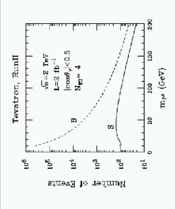
Figure 6: Projected $gg\to P^{0}\to\gamma\gamma$ signal rate $S$ and irreducible background rate for an integrated luminosity of 2 $fb^{-1}$ at Tevatron Run II; from [170].

(ii) Color-triplet PNGB’s: the $P_{3}$ Leptoquarks

As we have seen, the spectrum of the Farhi-Susskind TC model includes color-triplet technipions, with leptoquark quantum numbers [43, 101, 156]. These objects, $P_{3}$’s, would be predominantly resonantly pair-produced through a color-octet techni-$\rho$ ($V_{8}$) coupled either to gluons, or through octet vector dominance mixing (VMD) with the ordinary gluon. The latter case assures a signal in $q\bar{q}$ annihilation provided the $V_{8}$ can be excited.

$P_{3}$’s decay (via ETC [172] [173]) preferentially to third-generation quarks and leptons. At leading order, the leptoquark pair production cross section depends only on the masses ($M_{V_{8}},M_{P_{3}}$) and the $V_{8}$ decay width ($\Gamma_{V_{8}}$). The latter depends, in turn, on masses, on the size of the TC group $N_{TC}$ and on the mass-splitting between the color-octet and color-triplet technipions ($\Delta M$). While we would expect that $V_{8}$ VMD with the gluon would provide the largest contribution to the hadronic production of colored PNGB’s, provided the $V_{8}$ pole is within reach of the machine energy, at this writing there is no study of this contribution and its effects.

EHLQ [101], and more recently W. Skiba [174], have studied of hadron collider signatures of colored PNGB’s, without the $V_{8}$ resonant enhancement. Possible processes in which colored PNGBs can be produced in hadron colliders are: (i) Gluon-gluon and quark–anti-quark annihilations as sources of PNGB pair production; (ii) Quark-gluon fusion producing single PNGB’s; (iii) anomalous couplings to two gluons producing single PNGB’s. Direct PNGB couplings to fermions (through ETC effects) are typically too small to give significant cross sections. The $V_{8}$ VMD is neglected in the present discussion, and we know of no reference in the literature in which its effects are included.

The cross section for the pair production of colored PNGB’s has been calculated in Ref. [103] for the general case of pseudo(scalar) particles in any representation of $SU(3)_{color}$. Quark anti-quark annihilation yields

$$\frac{d\sigma}{d\hat{t}}(q\bar{q}\rightarrow PP)=\frac{2\pi\alpha_{s}^{2}}{9\hat{s}^{2}}\,k_{d}\beta^{2}(1-z^{2})$$ (2.73)

and $g-g$ annihilation gives

$$\frac{d\sigma}{d\hat{t}}(gg\rightarrow PP)=\frac{2\pi\alpha_{s}^{2}}{\hat{s}^{2}}\,k_{d}\left(\frac{k_{d}}{d}-\frac{3}{32}(1-\beta^{2}z^{2})\right)\left(1-2V+2V^{2}\right).$$ (2.74)

where $k_{d}$ is the “Dynkin index” of the $d$-dimensional representation ($k_{3}=\frac{1}{2}$, $k_{8}=3$), $z$ the cosine of parton scattering angle in the center of mass system,

$$V=1-\frac{1-\beta^{2}}{1-\beta^{2}z^{2}}\ \ {\rm and}\ \ \beta^{2}=1-\frac{4m_{P}^{2}}{\hat{s}},$$

$\hat{s}$ and $\hat{t}$ are Mandelstam variables at the parton level. Using these formulae and parton distributions from Ref. [175] (set 1), Skiba obtains [174] production rates for leptoquarks, $P_{3}$, and octets, $P_{8}$, which agree with the results of Refs. [101] (see also Hewett et al. , [176]). As the cross-section for pair production of leptoquarks at LHC energies is sizeable (see Fig.(7)), the LHC can potentially observe leptoquarks with masses up to approximately $\sim 1$ TeV.

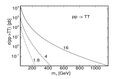
Figure 7: The cross section for pair production of leptoquarks in pp collisions, for $\sqrt{s}=$ 1.8, 4 and 16 TeV, (from W. Skiba [174]; $T=P_{3}$ in Skiba’s notation).

Figure 8: The cross section for pair production of color-octet PNGBs in pp collisions, for $\sqrt{s}=$ 1.8, 4 and 16 TeV, (from W. Skiba [174]; $\theta=P_{8}$ in Skiba’s notation).

(iii) Color-octet PNGB’s, $P_{8}$, and vector mesons $\rho_{T8}$

Due to color factors, the production cross sections for color octet $P_{8}$’s are an order of magnitude larger than for leptoquarks, as a comparison of Figures 7 and 8 reveals. The detection of $P_{8}$’s is, on the other hand, far more difficult. $P_{8}$’s typically decay into two hadronic jets, so that pair-produced $P_{8}$’s yield four-jet final states. QCD four-jet production is the main source of background, and it is overwhelmingly large. We mention here two suggestions from the literature as to how $P_{8}$ states might be detected. One involves using special cuts and kinematic variables to bring out the $P_{8}$ signal in four-jet final states. The other turns to a single-production of $P_{8}$ and a rarer $P_{8}$ decay mode with lower backgrounds.

Chivukula, Golden and Simmons Ref. [177, 178] have evaluated the possibility of detecting new colored particles at the Tevatron and LHC in multi-jet final states. The analysis begins with estimating the QCD multi-jet background [179, 180, 181, 182, 183, 184] and calculating the signal from heavy particle decays. Isolation and centrality cuts must be applied to ensure all jets are detectable. Then appropriate kinematic variables must be chosen to make the signal stand out cleanly above background.

The following strategy allows one to pull a $P_{8}$ signal out of the large QCD background [177], as illustrated in Figure 9. For each four-jet event, consider all possible pairwise partitions of the jets. Choose the partition for which the two pairs are closest in invariant mass, and define the “balanced pair mass,” $m_{bal}$, as the average of the two masses. The signal cross-section will cluster about $m_{bal}=m_{new\ particle}$ while the background will not. Imposing a large minimum-$p_{T}$ cut on the jets further enhances the signal; the background is peaked at low $p_{T}$ due to infrared QCD singularities.

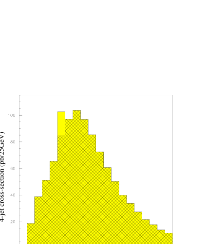
Figure 9: Four-jet rate $\frac{d\sigma}{dm_{bal}}$ at a $17$ TeV collider with $p_{T}^{min}$ of $100$ GeV. QCD background (hatched) and $240$ GeV technipion signal are shown. No resolution effects included (from ref. [177]).

Analyses of this kind indicate that real scalar color-octet particles with masses as high as $325$ GeV should be visible at the LHC if a $p_{T}$ cut of about $\sim 170$ GeV is employed [169]. The lower end of the visible mass range depends strongly on just how energetic ($p_{T}^{min}$) and well-separated ($\Delta R$) jets must be in order for an event to be identified as containing four distinct jets. Discovery of color-octet scalars at the Tevatron is likely to be possible, albeit difficult, in a reduced mass range [177].

Figure 10: Partial widths for the decay of $P_{8}^{0\prime}$ into gluon-gluon (solid line), $\bar{b}b$ (dashed line), $\bar{t}t$ (dotted line) and $Z$-gluon (dot-dashed line) in the Farhi-Susskind model [169].

An alternative strategy is to use processes with smaller backgrounds, such as single-production followed by a rarer decay mode. At hadron colliders, the widths relevant for single production and decay of the $P_{8}^{0\prime}$ of the Farhi-Susskind model are [169, 185] :

$$\Gamma(P_{8}^{0\prime}\rightarrow q\bar{q}) = \frac{3}{16\pi}\frac{m_{q}^{2}}{F^{2}}m_{P}\left(1-4m_{q}^{2}/m_{P}^{2}\right)^{3/2}$$

$$\Gamma(P_{8}^{0\prime}\rightarrow gg) = \frac{5\alpha_{s}^{2}}{24\pi^{3}}\left(\frac{N}{4}\right)^{2}\frac{m_{P}^{3}}{F^{2}}\;$$

$$\Gamma(P_{8}^{0\prime}\rightarrow g\gamma) = \left(\frac{Neg_{s}}{4\pi F}\right)^{2}\frac{m_{P}^{3}}{576\pi}\;.$$ (2.75)

Figure 10 gives the decay widths of the $P_{8}^{0\prime}$ in the Farhi-Susskind model. Figure 11 illustrates gluon fusion production at the LHC and we see that the rate of single $P_{8}^{0\prime}$ production is high at a hadron collider. However, the signal in the primary decay channels (gluon or b-quark pairs) is swamped by QCD background. If the PNGB mass is above the $t\bar{t}$ threshold, the decay mode $P\rightarrow t\bar{t}$ becomes dominant and may alter the standard QCD value of the $t\bar{t}$ cross section and $t\bar{t}$ spin correlations. The decay channel $P\to g\gamma$ [186, 185] holds some promise for the models of “low-scale” TC discussed in Section 3.5; however the PNGB’s of the Farhi-Susskind TC model are not likely to be visible in this mode.

Figure 11: Differential cross section at $y=0$ for single production of $\rho_{T8}^{0\prime}$ (solid line) and $P_{8}^{0\prime}$ (dashed line) at the LHC in femtobarns [169].

The $\rho_{T8}^{0\prime}$ coupling to $gg$ and $q\bar{q}$ can be estimated by assuming that it mixes with the gluon under a generalized vector meson dominance (VMD). VMD applies to the $gg\rightarrow\rho_{T8}^{0\prime}$ process as well as the $q\bar{q}\rightarrow\rho_{T8}^{0\prime}$ process ref. [159]. The partial widths relevant for $\rho_{T8}^{0\prime}$ production at hadron colliders in the narrow width approximation are [169]:

$$\Gamma(\rho_{T8}^{0\prime}\rightarrow gg) = \frac{\alpha_{s}^{2}}{2\alpha_{\rho}}m_{\rho}$$ (2.76)

$$\Gamma(\rho_{T8}^{0\prime}\rightarrow q\bar{q}) = \frac{5\alpha_{s}^{2}}{6\alpha_{\rho}}m_{\rho}$$ (2.77)

Figure 11 compares the single production cross section of the $\rho_{T8}^{0\prime}$ and $P_{8}^{0\prime}$ at the LHC.

If kinematically allowed the dominant decay mode of $\rho_{8T}^{0\prime}$ is into two colored PNGB [169]:

$$\Gamma(\rho_{8T}^{0\prime}\rightarrow P_{8}P_{8})=\frac{\alpha_{\rho_{T}}}{4}\;m_{\rho}\;\left(1-4m_{P}^{2}/m_{\rho}^{2}\right)^{3/2}.$$ (2.78)

In this case the $\rho_{T8}^{0\prime}$ contributes strongly to the cross section for color-octet PNGB pair production discussed in above and improves the signal.

If the $\rho_{T8}$ are light, e.g. in low-scale models (Section 3.5), there can be a sizeable cross section for their pair production. Näively, well above the pair-production threshold one expects: [169] :

$$\frac{\sigma(pp\rightarrow\rho_{T8}+X)}{\sigma(pp\rightarrow\rho_{T8}\rho_{T8}+X)}\simeq\frac{1}{g_{\rho_{T}}^{2}}\simeq\frac{1}{40}.$$ (2.79)

Note that all types of colored vector resonances can be pair-produced, whereas the isosinglet $\rho_{T8}^{0\prime}$ dominates single production. Hence, pair production, unlike single production, can result in interesting decays to longitudinal electroweak gauge bosons. One may also expect spectacular $8$–jet events whose kinematics distinguish them from the QCD background, as in the case of color-octet PNGB pair production.

The $\rho_{T8}$ can significantly affect the invariant mass distribution of $\bar{t}t$ final states [104]. Through gluonic vector dominance processes like $\bar{q}q\rightarrow g+\rho_{T8}\rightarrow\bar{t}t$ the gluon and $\rho_{T8}$ add coherently. Significant mass imits can be placed from the Tevatron in Run II (this process has a direct analogue in Topcolor, where $\rho_{T8}$ becomes the coloron [187]).

(iv) Non-Resonant Production and Longitudinal Gauge Boson Scattering

At the next level, below resonance production, we expect gauge boson fusion through techniquark loops (including anomalous loops) into techni-vector mesons and/or techni-pions. This can include gluon fusion [135], [136], [137], [138] at machines such as the LHC, or $W-W$ fusion at an LHC or LC (see section 2.3.4) [139], [140], [141], [142], [143]. Scattering of the longitudinal electroweak modes, $V_{L}V_{L}\to V_{L}V_{L}$, is especially important (see Section 2.2.3). These processes involve all possible spin and isospin channels simultaneously, and can proceed through scalar and vector resonances or non-resonant channels.

(v) Rescattering

An alternative way of finding color-octet technipions is to detect them after they have re-scattered into pairs of $W$ or $Z$ particles. For example, in the Farhi-Susskind TC model the production of gauge boson pairs through gluon fusion includes a potentially sizeable [188] contribution from loops of colored technipions through the process $P_{8}^{0,\pm}P_{8}^{0,\pm}\to WW$ or $ZZ$. This may prove to be a very useful diagonostic. If colored technipions are first detected in 4-jet final states, their association with electroweak symmetry breaking will not be obvious. However, the combination of their discovery with the observation of a large number of gauge-boson pairs may permit us to deduce that the colored scalars are PNGB’s of the symmetry breaking sector [189].

Figure 12: The $ZZ$ differential cross section in nb/GeV vs. $M_{ZZ}$ in a toy $O(N)$ scalar-model with three color-octet PNGBs (upper curve), and the continuum $q\bar{q}$ annihilation background (lower curve). A pseudo-rapidity cut $|\eta|<2.5$ is imposed on the final state $Z$’s. From [189]

The contribution of loops of colored technipions to the production of gauge-boson pairs through gluon fusion was calculated to leading order in chiral perturbation theory in ref. [188]. Unfortunately, general considerations [190, 191] show that in theories with many Nambu–Goldstone bosons, chiral perturbation theory breaks down at very low energies. In the Farhi-Susskind model, for example, chiral perturbation theory breaks down at a scale of order 440 GeV! Hence only a qualitative estimate of the signal size is possible. Figure 12 shows the $ZZ$ differential cross section as a function of $ZZ$ invariant mass at the LHC in a toy $O(N)$ scalar-model [189]; model parameters were chosen so the signal size is representative of Farhi-Susskind TC. Note that there are almost an order of magnitude more events due to gluon fusion than due to the continuum $q\bar{q}$ annihilation for $ZZ$ invariant masses between 300 GeV and 1 TeV. The observation of such a large two gauge-boson pair rate at a hadron collider would be compelling evidence that the EWSB sector couples to color.

2.3.4 Production and Detection at $e^{+}e^{-}$ Colliders

(i) pair-production of EW bosons

The $s$-channel process $e^{+}e^{-}\to WW$ is an effective probe of strong electroweak symmetry breaking, especially for physics with a vector resonance [192, 193, 134, 194]. A $500$ GeV linear collider with only 80 fb^-1 of integrated luminosity would already be sensitive to radiative corrections induced by vector resonances with masses up to about 2 TeV, but would not be able to observe off-resonance contributions to $WW$ production (see Figure 13). With 500 fb^-1 of integrated luminosity, even the non-resonant or low-energy-theorem contributions would become distinguishable from Standard Model expectations, as illustrated in Figure 14. A higher-energy $e^{+}e^{-}$ collider would have even greater search potential. With $\sqrt{s}$=1.5 TeV and an integrated luminosity of 190 fb^-1, it should be possible to distinguish the radiative effects of a very heavy techni-$\rho$ or a non-resonant amplitude from those of the standard model with a light Higgs boson; the 4 TeV (6 TeV) techni-$\rho$ corresponds to a 6.5$\sigma$ (4.8 $\sigma$) signal. At a slightly higher integrated luminosity of 225 fb^-1, it would be possible to obtain 7.1$\sigma$, 5.3$\sigma$ and 5.0$\sigma$ signals for a 4 TeV techni-$\rho$, a 6 TeV techni-$\rho$, and non-resonant contributions, respectively.

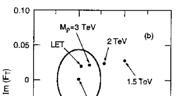
Figure 13: Sensitivity of a 500 GeV LC with 80 $fb^{-1}$ of data to $M_{\rho_{T}}$ via the $W$–boson form factor; from Ref.[193]. The predicted values for a 3-TeV $\rho_{T}$ or non-resonant scattering (LET) lie within the 95% c.l. curve for the prediction of the Standard Model; these cases cannot, then be reliably distinguished. Lighter $\rho_{T}$ give predictions which differ significantly from those of the Standard Model.

Figure 14: Sensitivity of a 500 GeV LC with 500 $fb^{-1}$ of data to $M_{\rho_{T}}$ via the $W$–boson form factor; from Ref.[194]. The predicted values for a 2.5-TeV $\rho_{T}$ or non-resonant scattering (LET) now lie outside 95% c.l. curve for the prediction of the Standard Model.

The $WW$ fusion processes are complementary to the $s$-channel $W^{+}W^{-}$ mode since they involve more spin-isospin channels (the $I=0$ and $I=2$ channels). For an $e^{+}e^{-}$ collider at $\sqrt{s}=1.5$ TeV with 190 fb^-1 of data, the $W^{+}W^{-}/ZZ$ event ratio can be a sensitive probe of a strongly-interacting electroweak sector [134, 195, 196, 197, 198] as illustrated in Table 4. Statistically significant signals are found for a 1 TeV scalar or vector particle. There is also about a 6$\sigma$ signal for non-resonant (low-energy-theorem) amplitudes via the $W^{+}W^{-}\to ZZ$ channel alone. For an $e^{-}e^{-}$ collider with the same energy and luminosity, the non-resonant-amplitude signal rate for the $\nu\nu W^{-}W^{-}$ ($I=2$) channel [197] is similar to that for $e^{+}e^{-}\to\bar{\nu}\nu ZZ$, as anticipated from symmetry arguments, while the background rate is higher [134]. The signals are doubled for an $e^{-}_{L}$ polarized beam (or quadrupled for two $e^{-}_{L}$ beams), whereas the backgrounds increase by smaller factors. A 2 TeV $e^{+}e^{-}$ linear collider would increase the signal rates by roughly a factor of 2–2.5.

channels	SM	Scalar	Vector	LET
	$m_{H}=1$ TeV	$M_{S}=1$ TeV	$M_{V}=1$ TeV
$S(e^{+}e^{-}\to\bar{\nu}\nu W^{+}W^{-})$	160	160	46	31
$B$(backgrounds)	170	170	4.5	170
$S/\sqrt{B}$	12	12	22	2.4
$S(e^{+}e^{-}\to\bar{\nu}\nu ZZ)$	120	130	36	45
$B$(backgrounds)	63	63	63	63
$S/\sqrt{B}$	15	17	4.5	5.7
$S(e^{-}e^{-}\to\nu\nu W^{-}W^{-})$	27	35	36	42
$B$(backgrounds)	230	230	230	230
$S/\sqrt{B}$	1.8	2.3	2.4	2.8

Table 4: Total numbers of $W^{+}W^{-}\to 4$-jet and $ZZ\to 4$-jet signal $S$ and background $B$ events calculated for a 1.5 TeV LC with integrated luminosity 200 fb^-1. Results are shown for the SM, for strongly-coupled models with scalar or vector resonances and for low-energy-theorem (LET) scattering. Events are summed over the mass range $0.5<M_{WW}<1.5$ TeV except for the $W^{+}W^{-}$ channel with a narrow vector resonance in which $0.9<M_{WW}<1.1$ TeV. The statistical significance $S/\sqrt{B}$ is also given. For comparison, results for $e^{-}e^{-}\to\nu\nu W^{-}W^{-}$ are also presented, for the same energy and luminosity. The hadronic branching fractions of $WW$ decays and the $W^{\pm}/Z$ identification/misidentification are included. From ref. [134].

When both the both the pair production and gauge boson fusion processes are taken into account, the direct signal of a strongly-coupled symmetry-breaking sector is generally stronger at a high-energy linear collider than at the LHC; Figure 15.

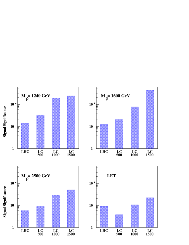
Figure 15: Direct strong symmetry breaking signal significance in $\sigma$’s for various masses $M_{\rho}$ of a vector resonance in $W_{L}W_{L}$ scattering [194]. The numbers below the “LC” labels refer to the center-of-mass energy of the linear collider in GeV. The luminosity of the LHC is assumed to be 300 $fb^{-1}$, while the luminosities of the linear colliders are assumed to be 500, 1000, and 1000 $fb^{-1}$ for $\sqrt{s}$=500, 1000, and 1500 GeV respectively. The lower right hand plot “LET” refers to the case where no vector resonance exists at any mass in strong $W_{L}W_{L}$ scattering.

A strongly–coupled electroweak symmetry breaking sector can also be investigated [134] at photon–photon colliders in the modes $\gamma\gamma\to ZZ$, $\gamma\gamma\to W^{+}W^{-}$, $\gamma\gamma\to W^{+}W^{-}W^{+}W^{-}$, and $\gamma\gamma\to W^{+}W^{-}ZZ$. While irreducible backgrounds in the first two cases are severe, the four-boson final states seem more promising [199]. To be sensitive to a heavy scalar resonance (e.g. heavy Higgs) with a mass up to 1 TeV would require a 2 TeV $e^{+}e^{-}$ collider with luminosity of 200 fb^-1 [200], [201]. A $1.5$ TeV linear collider running in the $\gamma\gamma$ mode is found to be roughly equivalent to a $2$ TeV $e^{+}e^{-}$ collider for the purpose of studying strongly-interacting ESB physics [200, 201] (the correspondence scales roughly as $\sqrt{s_{\gamma\gamma}}\sim 0.8\sqrt{s_{ee}}$).

(ii) colorless neutral PNGBs, $P^{0},P^{0}{}^{\prime}$

A light enough neutral PNGB can be singly produced at an $e^{+}e^{-}$ collider via the axial-vector anomaly [202, 203] which couple the PNGB to pairs of electroweak gauge bosons. At LEP I the PNGB, $P^{a}$, would have been primarily produced [204, 205, 206] through an anomalous coupling to the $Z$ boson and either a photon ($Z\to\gamma P^{a}$) or a second, off-shell $Z$ boson ($Z\to Z^{*}P^{a}$). At the higher center of mass energies of LEP II, PNGBs over a wider range of masses could have been produced through $s$-channel $\gamma^{*}/Z^{*}$ exchange and through a $2\to 3$ production mechanism [207, 170].

If the TC group is $SU(N_{T})$, the anomalous coupling between the PNGB and the gauge bosons $G_{1}$ and $G_{2}$ is given, as for the QCD pion, by [99, 208, 209]

$$N_{T}A_{G_{1}G_{2}}\frac{g_{1}g_{2}}{2\pi^{2}F_{T}}\epsilon_{\mu\nu\lambda\sigma}k^{\mu}_{1}k^{\nu}_{2}\varepsilon^{\lambda}_{1}\varepsilon^{\sigma}_{2}\ ,$$ (2.80)

where $N_{T}$ is the number of technicolors, $A_{G_{1}G_{2}}$ is the anomaly factor (see below), the $g_{i}$ are the gauge couplings of the gauge bosons, and the $k_{i}$ and $\varepsilon_{i}$ are the four-momenta and polarizations of the gauge bosons.

The model-dependent value of the anomaly factor is calculated in  [99], [208], [209]. The dominant production mode for a PNGB at LEP I was generally the $Z\to\gamma P^{a}$ process [204] which has a branching ratio of order $10^{-5}$

$$\Gamma_{Z^{0}\to\gamma P^{a}}=2.3\times 10^{-5}{\rm GeV}\left(\frac{123{\rm GeV}}{F_{T}}\right)^{2}\left(N_{T}A_{\gamma Z^{0}}\right)^{2}\left(\frac{M_{Z^{0}}^{2}-M_{P^{a}}^{2}}{M_{Z^{0}}^{2}}\right)^{3}\ .$$ (2.81)

The final states contain a hard, mono-energetic photon, along with the decay products of $P^{a}$. Production in combination with an off-shell $Z^{0}$ is harder to observe. An upper bound on the decay width of the process $Z^{0}\to Z^{0*}P^{a}\to P^{a}f\bar{f}$ is given by  [205, 210]. One expects branching ratios of order $10^{-7}$ to $10^{-6}$, depending on the process of interest. At LEP II and an NLC, production modes include $e^{+}e^{-}\to\gamma^{*},Z^{*}\to\gamma^{(*)}P^{a},Z^{(*)}P^{a}$ and the 2-to-3 process, $e^{+}e^{-}\to e^{+}e^{-}P^{a}$ [207].

In the minimal models, the PNGB’s decay back into electroweak bosons. Which decays are allowed or dominant depends on the values of the anomaly factors. For example, a neutral colorless PNGB produced by $Z$-decay can certainly decay to an off-shell $Z$ plus another electroweak gauge boson (photon or $Z$). It may also be able to decay to a pair of photons; if allowed, this mode dominates over decays via off-shell $Z$’s. In any given non-minimal TC model, the dominant decay mode of the neutral PNGB’s depends both on the gauge couplings of the technifermions and on any interactions coupling technifermions to ordinary fermions. If some technifermions are colored, the PNGB may have an anomaly coupling allowing it to decay to gluons. If the PNGB gets its mass from effective four-fermion interactions (e.g. due to extended TC), then it will be able to decay to an $f\bar{f}$ pair. Finally, in some models, the PNGB may decay dominantly to particles in an invisible sector.

Searches for the neutral PNGB’s at LEP I and LEP II were sensitive only to PNGB’s with small technipion decay constants and large anomaly factors. The $P^{a}$ of the Farhi-Susskind model are invisible at these colliders. However, data from the LEP experiments is able to test the properties of the PNGB’s of various extended models, such as the Appelquist-Terning model [211], the Manohar-Randall weak isotriplet model [204], Lane’s low-scale TC model [212, 213], and the Lane-Ramana multiscale model [156]. Details about all of the constraints are available in Ref. [210]; a summary for a few walking TC models will be given in Section 3. For now, we turn to the possibility of direct searches at higher-energy linear colliders.

The possibility of searching at a $1$ TeV Linear Collider for a generic neutral $P^{0(^{\prime})}$ decaying predominantly to the heaviest available fermions

$$e^{+}e^{-}\to P^{0}_{T}\gamma \to t\bar{t}\gamma\to b\bar{b}W^{+}W^{-}\gamma\qquad M_{P}>2m_{t}$$ (2.82)

$$\to b\bar{b}\gamma\qquad\qquad M_{\Pi}<2m_{t}.$$

was studied in ref. [214]. The signal events will stand out from the background due to the hard monochromatic photon recoiling against the PNGB decay products. Based on a Monte Carlo simulation of signal and background, ref. [214] finds that for models with $N_{T}=3$ and $f_{T}=123$, the $P^{0}{}^{\prime}$ can be excluded at the 95% c.l. up to a mass of 646 GeV and could be discovered at the 5-sigma level up to a mass of 452 GeV. The $P^{0}$ production rate appears too small to allow discovery in the models examined. These results are illustrated in Figures 16 and 17.

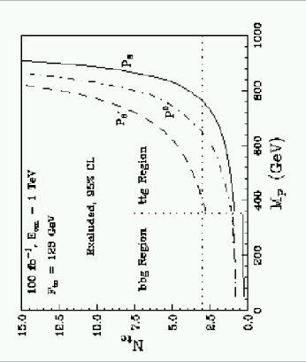
Figure 16: Projected 95% c.l. exclusion reach for electrically neutral PNGB as a function of mass and number of technicolors at a 1 TeV LC [214].

The electrically neutral color-octet $P_{8}^{0(^{\prime})}$ will be singly produced in association with a gluon through the anomalous coupling of the PNGB to the gluon and a photon or $Z$ boson. Provided that the PNGB decays to the heaviest available fermion pair, the production and decay chain will look like [214]

$$e^{+}e^{-}\to P^{0}_{T8}g \to t\bar{t}g\to b\bar{b}W^{+}W^{-}g\qquad M_{P8}>2m_{t}$$ (2.83)

$$\to b\bar{b}g\qquad\qquad M_{P8}<2m_{t}.$$

Characteristics that will help distinguish the signal events from those of the $q\bar{q}g$ background are monochromaticity of the gluons in the signal events are monochromatic and their large spatial separation from the PNGB decay products. The left-right asymmetries and $t\bar{t}$ spin correlations will also differ from those of the background distributions. Based on a Monte Carlo simulation of signal and background, ref. [214] asserts that the electrically neutral color-octet PNGB can be excluded or discovered for any realistic values of $N_{TC}$ provided that $M_{P}<2m_{t}$. For higher-mass PNGB, finding the $P_{T8}^{0^{\prime}}$ will require including events with hadronic $W$ decays for $N_{TC}<7$. For the specific case $N_{TC}=3$, it will be possible for a 1 TeV LC to exclude a $P_{T8}^{0}\ (P_{T8}^{0^{\prime}})$ of mass less than 761 (404) GeV at 95% c.l. or to discover a $P_{T8}^{0}$ with five-sigma significance for $M<524$ GeV [214]. The exclusion and discovery limits are shown in Figures 16 and 17.

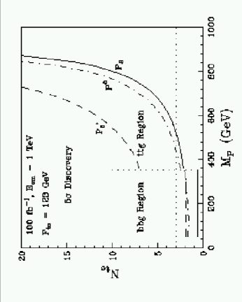
Figure 17: Projected 5-sigma discovery reach for electrically neutral PNGB as a function of mass and number of Technicolors at a 1 TeV LC [214].

The ability of an LC to study the lightest PNGB of a particular model [171] has been probed in ref.[170]. They find that the process $e^{+}e^{-}\to P^{0}\gamma$ would allow discovery so long as the PNGB mass was not close to $M_{Z}$ and for $N_{T}\geq 3$. Moreover, if running in $\gamma\gamma$ mode, the process $\gamma\gamma\to P^{0}\to b\bar{b}$ could not only allow detection of a PNGB with mass between 10% and 70% of $\sqrt{s}$, but would also provide more precise information about model parameters. A muon collider could in principle help determine the couplings of a PNGB in greater detail.

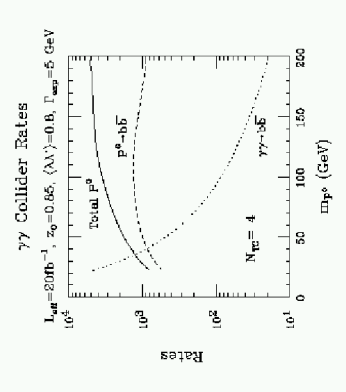
Figure 18: Projected $P^{0}$ production rate (solid), rate including PNGB decay to $b\bar{b}$ (dashed), and irreducible $\gamma\gamma\to b\bar{b}$ background (dotted) for $\gamma\gamma$ collisions at $\sqrt{s}=500$ GeV with integrated luminosity of 20 $fb^{-1}$ [170].

The production and detection of the $\eta_{T}^{\prime}$ state has been studied in [92] and [93], the latter with emphasis on the laser back-scattering technique at an $e^{+}e^{-}$ LC [215].

(iii) colorless charged PNGBs, $P^{\pm}$

Electrically charged PNGB’s would be abundantly pair-produced at a high-energy, high-luminosity linear electron-positron collider. In terms of the electromagnetic point cross section $\sigma_{o}=4\pi\alpha^{2}(s)/3s$, the continuum cross-section for producing $P_{0}^{+}P_{0}^{-}$ pairs at an NLC is $0.30\beta^{3}\sigma_{o}$, where $\beta$ is the c.m. frame velocity of $P_{0}^{\pm}$ [214]. Assuming the $P_{0}^{\pm}$ decay dominantly to $tb$ pairs, the final state contains a pair of on-shell W bosons and four b quarks. The leading background comes from $t\bar{t}g^{*}$ events where the off-shell gluon materializes as a $b\bar{b}$ pair; the cross-section for this process is less than a tenth of the $t\bar{t}$ production cross-section of 1.9$\sigma_{o}$. Given a detector with good angular coverage and high efficiency for detection of the b-jets, it should be possible to detect $P^{\pm}_{0}$ with a mass below about 0.45$\sqrt{s}$ at the five-sigma significance level [214]. Similarly, the large electromagnetic pair-production cross-section and moderate backgrounds for pair-production of $P^{\pm}_{T8}$ should make 5-sigma significance discovery possible out to a mass of approximately 0.49 $\sqrt{s}$ [214].

As seen from the discussion of section 2.2.4, the $\rho_{T}^{0}$ will couple via VMD to any electromagnetic current (or to the weak neutral current, which can include $\omega_{T}$). VMD production on the narrow resonances will produce dramatic signatures in the conventional final states as in $e^{+}e^{-}\rightarrow(\rho_{T},\omega_{T})\rightarrow(WW+ZZ,W\pi+ZP,PP)$. Such processes have been discussed in the context of muon colliders, where the better beam energy resolution is an advantage, in ref.[157].

In contrast, the work of ref [216] suggests that it will be difficult to detect the effects of charged technipions on single top production at an $e\gamma$ collider in the process $e\gamma\to tb\nu$.

3 Extended Technicolor

3.1 The General Structure of ETC

A realistic Technicolor model must address the flavor problem. That is, it must incorporate a mechanism for generating quark and lepton masses and the various weak mixing angles, together with CP-violation. This implies that the ordinary quarks and leptons of the Standard Model need to couple to the technifermion condensate that breaks the electroweak symmetry. There must also be a mechanism for violating the conserved techni-baryon quantum number: techniquarks must be able to decay, since stable techni-baryonic states are cosmologically problematic [64].

The classic way to fulfill these requirements is to extend the Technicolor gauge interactions to include additional gauge bosons coupling both to ordinary and Technicolored fermions. The extended interactions are part of a large gauge group which necessarily breaks down to its Technicolor subgroup at an energy above the scale at which the Technicolor coupling becomes strong, $\Lambda_{TC}$.

The construction of the first theories of “Extended Technicolor” (ETC) is due to Eichten & Lane [173] and Dimopoulos & Susskind [172]. Their work, and the papers which followed in the early 1980’s, especially [208], [100], [217] [99], [78], [218], flesh out the general scheme and identify the challenges. We will summarize the major issues, indicate trends in modern model-building, and refer the reader to the literature for further detail.

3.1.1 Master Gauge Group ${\cal{G}}_{ETC}$

The kinds of new interactions that are required for ETC involve transition couplings of technifermions $Q_{L,R}$ into the ordinary quarks and leptons, $\psi_{L,R}$. Currents of the form $\bar{Q}_{L,R}\gamma_{\mu}\psi_{L,R}$ are therefore required, coupling to the new ETC gauge bosons. In a full theory we assume a large gauge group ${\cal{G}}_{ETC}$ which contains all of the desired currents of the form $\bar{Q}Q$, $\bar{Q}\psi$ and $\bar{\psi}\psi$. A simple generalization is a blockwise imbedding of $SU(N_{TC})$ into $SU(N_{ETC})$ with $N_{ETC}>N_{TC}$. Clearly $N_{ETC}$ must be large enough to accomodate representations containing both $\psi$’s and $Q$’s.

For example, consider how this imbedding might work in the minimal model. The minimal model includes one weak doublet of technifermions ($N_{D}$ = 1) and a typical choice of Technicolor group $N_{TC}=4$. ETC must couple the technifermions to all $12$ left-handed electroweak doublets of ordinary quarks and leptons and all $12$ singlets. Then we should think of the ordinary fermions of each generation as falling into 3 doublets of quarks and one of leptons under the gauged $SU(2)_{L}$ and an analogous set of doublets under a global $SU(2)_{R}$. This yields an ETC scheme with a gauge group ${\cal{G}}_{ETC}=SU(16)\times SU(2)_{L}\times SU(2)_{R}\times U(1)$. Both $SU(N_{TC})$ and $SU(3)_{c}$ are imbedded into $SU(16)$; hypercharge arises as $Y/2=I_{3R}+(B-L)/2$, where $B-L$ is a diagonal generator in $SU(16)$. The fermions form two fundamental 16 multiplets; one of them:

$$(Q_{c},Q_{k},Q_{m},Q_{y},\psi_{r}^{1},\psi_{g}^{1},\psi_{b}^{1},\psi_{r}^{2},\psi_{g}^{2},\psi_{b}^{2},\psi_{r}^{3},\psi_{g}^{3},\psi_{b}^{3},\psi_{lep}^{1},\psi_{lep}^{2},\psi_{lep}^{3})_{L}$$

$${\rm c,k,m,y=Technicolors;\ \ \ r,g,b=colors}$$

is a doublet under the electroweak group $SU(2)_{L}$, and a singlet under $SU(2)_{R}$, a $(2,1)$; the other is a $(1,2)$. The Technicolor condensate will therefore break both the $SU(2)_{L}$ and the $SU(2)_{R}$. For the Farhi-Susskind model, an analogous ETC extension might be to a gigantic gauge group placing all of the quarks and leptons and techniquarks (including each Technicolor copy) into a single multiplet of a compact gauge group, e.g., $SU(56)$. Here the full Standard Model gauge interactions themselves would be subgroups of the master group $SU(56)$. Clearly a large variety of models are possible, and we will describe several general approaches to building consistent models in this Section (several variant schemes are also reviewed in [57]).

Starting from a high-energy theory based on a master gauge group ${\cal{G}}_{ETC}$, it is necessary to arrive at a low-energy theory in which the only surviving gauge groups are those of Technicolor and the Standard Model. The group ${\cal{G}}_{ETC}$ has generators, $T^{a}$, which form a Lie Group,

$$[T^{a},T^{b}]=if^{abc}T^{c}$$ (3.85)

The Technicolor gauge group ${\cal{G}}_{TC}$ must be a subgroup of ${\cal{G}}_{ETC}$, since the $\psi$’s do not carry Technicolor, while the $Q$’s do. Then ${\cal{G}}_{ETC}$ must undergo symmetry breaking at a scale $\Lambda_{ETC}$ down to its subgroup ${\cal{G}}_{TC}$:

$${\cal{G}}_{ETC}\rightarrow{\cal{G}}_{TC}\times...\qquad\makebox{at $\Lambda_{ETC}$}.$$ (3.86)

where the ellipsis denotes other factor groups, including perhaps the full Standard Model $SU(3)\times SU(2)\times U(1)$. This leaves the Technicolor gauge bosons (generators denoted $\tilde{T}^{a}$) massless, and elevates all of the coset ETC gauge bosons to masses of order $\Lambda_{ETC}$. Indeed, the breaking may proceed in a more complicated way, e.g., it may occur in $n$ steps ${\cal{G}}_{ETC}\rightarrow{\cal{G}}_{1}\rightarrow{\cal{G}}_{2}\rightarrow...{\cal{G}}_{n-1}\rightarrow{\cal{G}}_{TC}$. A class of models in which this symmetry-breaking sequence is achieved dynamically is known as “Tumbling Gauge Theories” [219, 220, 221, 222, 223, 224, 225]. Typically, at each step, the subgroup will evolve and become strong, permitting new condensates to form, which further break the theory into the next subgroup. This occurs repetitively at different scales, and may in principle be a way of generating the mass hierarchy for quarks and leptons of different flavors. Another possibility is that there are fundamental scalars associated with supersymmetry at some high energy scale, and the breaking of ${\cal{G}}_{ETC}$ (whether single or sequential) can be driven by a Higgs mechanism (see Section 3.7).

3.1.2 Low Energy Relic Interactions

While the only elements of the original ETC gauge group that survive at low energies are the generators of the Technicolor and Standard Model gauge groups, the low-energy phenomenology of these models includes additional effects caused by the broken ETC generators. On energy scales $\mu\mathrel{\vbox{\hbox{$<$}\nointerlineskip\hbox{$\sim$}}}\Lambda_{ETC}$ exchange of the heavy ETC bosons corresponding to those broken generators produces three types of effective contact interactions among the ordinary and technifermions:

$$\bar{\alpha}_{ab}\frac{\bar{Q}\gamma_{\mu}\bar{T}^{a}Q\bar{Q}\gamma^{\mu}\bar{T}^{b}Q}{\Lambda_{ETC}^{2}}+\bar{\beta}_{ab}\frac{\bar{Q}\gamma_{\mu}\bar{T}^{a}\psi\bar{\psi}\gamma^{\mu}\bar{T}^{b}Q}{\Lambda_{ETC}^{2}}+\bar{\gamma}_{ab}\frac{\bar{\psi}\gamma_{\mu}\bar{T}^{a}\psi\bar{\psi}\gamma^{\mu}\bar{T}^{b}\psi}{\Lambda_{ETC}^{2}}$$ (3.87)

Here the $\alpha$, $\beta$ and $\gamma$ are coefficents that are contracted with generator indices and their structure depends upon the details of the parent ETC theory. In the $\bar{T}^{a}$ we include chiral factors such as $(1\pm\gamma^{5})/2$ (i.e., the theory is flavor-chiral and the ETC generators have different actions on left- and right-handed fermions). We can now Fierz rearrange these operators to bring them into the form of products of scalar and pseudo–scalar densities. Upon Fierz rearrangement, we can pick out the generic terms of greatest phenomenological relevance:

$$\alpha_{ab}\frac{\bar{Q}T^{a}Q\bar{Q}T^{b}Q}{\Lambda_{ETC}^{2}}+\beta_{ab}\frac{\bar{Q}_{L}T^{a}Q_{R}\bar{\psi}_{R}T^{b}\psi_{L}}{\Lambda_{ETC}^{2}}+\gamma_{ab}\frac{\bar{\psi}_{L}T^{a}\psi_{R}\bar{\psi}_{R}T^{b}\psi_{L}}{\Lambda_{ETC}^{2}}+...$$ (3.88)

Note that after Fierzing we must include the identity matrix among the generators, which we do by extending the range of the generator indices to include zero: $\bf{1}\equiv T^{0}$.

Figure 19: The exchange of an ETC gauge boson allows a standard quark (or lepton) to communicate with the techniquark condensate, $\left\langle\overline{Q}Q\right\rangle$.

As a consequence of these generic terms we see that the physical effects of ETC go beyond generating the quark and lepton masses and mixings. On the positive side, ETC interactions, such as the $\alpha$-terms, can elevate the masses of some of the light Nambu-Goldstone bosons, such as the techniaxions, to finite nonzero values, essential to rendering models consistent with experiment. On the negative side, Extended Technicolor produces the $\gamma$-terms, four-fermion contact interactions amongst ordinary fermions of the same Standard Model gauge charges. This leads generally to flavor-changing neutral current effects in low energy hadronic systems, e.g., it can lead to dangerously large contributions to the $K_{L}K_{S}$ mass difference. Lepton number violation will also generally occur, leading to enhanced rates for $\mu\rightarrow e+\gamma$ and related processes. It is a difficult model-building challenge to limit these dangerous effects while generating adequately large quark and lepton masses to accomodate the heavier fermions, e.g., charm, $\tau$, $b$, and especially $t$. It is, moreover, important that the oblique electroweak corrections involving TC and ETC effects be under control [226], as will be discussed in Section 3.2. These and other phenomenological considerations have had a large influence on ETC model-building. We will look at explicit examples of models constructed to address such questions in Section 3.3.

3.1.3 The $\alpha$-terms: Techniaxion Masses.

The four-technifermion terms (with coefficients $\alpha$) can potentially solve a problem we encountered in the previous discussion of the minimal and Farhi-Susskind models in Section 2. Loops involving $\alpha$ term insertions, which represent ETC gauge boson exchange across a technifermion loop, with external PNGB’s (Fig.(20)) generally induce masses for the PNGB’s. This mechanism can elevate the masses of the undesireably light PNGB’s to larger values more consistent with experiment.

Figure 20: ETC gauge boson exchange across a fermion loop. This is an $\alpha$ term insertion leading to PNGB mass.

To see this explicitly, we can make use of an NJL or Georgi-Manohar model of the techniquark condensate, which instructs us to replace the techniquark bilinears in eq.(3.88) with the corresponding chiral fields (a discussion of the chiral dynamics of ETC may be found in [168], [231] ). Specifically one makes the replacement, motivated from the NJL approximation or QCD:

$$\bar{Q}_{aR}Q^{\dot{b}}_{L}\rightarrow cN_{TC}\Lambda_{TC}^{3}\Sigma_{a}^{\dot{b}}\qquad\qquad\Sigma_{a}^{\dot{b}}\equiv\exp(i\pi^{c}\tilde{T}^{c}/F_{T})_{a}^{\dot{b}}$$ (3.89)

where dotted indices are for $SU(2)_{L}$ and undotted are for $SU(2)_{R}$ and the $\tilde{T}^{a}$ are generators of the Technicolor subgroup of ${\cal{G}}_{ETC}$. This leads, through the diagram of Fig.(20), to a PNGB interaction term in the effective Lagrangian:

$$\sim\frac{\alpha_{ab}c^{2}N_{TC}^{2}\Lambda_{TC}^{6}}{\Lambda_{ETC}^{2}}\mathop{\rm Tr}(\Sigma T^{a}\Sigma^{\dagger}T^{b})$$ (3.90)

Expanding eq.(3.90) in the $\pi^{a}\tilde{T^{a}}$ we see that the induced technipion mass terms are:

$$\sim-\frac{\alpha_{ab}c^{2}N_{TC}^{2}\Lambda_{TC}^{6}}{\Lambda_{ETC}^{2}F_{T}^{2}}\mathop{\rm Tr}([\pi^{c}\tilde{T}^{c},T^{a}][T^{b},\pi^{d}\tilde{T}^{d}]$$ (3.91)

Those technipions associated with the Technicolor generators, $\tilde{T}^{a}$ that commute with ETC, i.e., for which:

$$[\tilde{T^{a}},T^{b}]=0\ ,$$ (3.92)

will have vanishing mass contributions from ETC. Technipions associated with the noncommuting generators, on the other hand, will generally receive nonzero ETC contributions to their masses of order $\sim N_{TC}\Lambda^{2}_{TC}/\Lambda_{ETC}$.

This situation is akin to that of QCD: the ${T^{a}}$ are analogues of the electric charge operator, and $\tilde{T^{a}}$ are the generators of nuclear isospin. The neutral pion of QCD is associated with a generator, $I_{3}$ that commutes with the electric charge, $Q=I_{3}+Y/2$, hence the neutral pion receives no contribution to its mass from electromagnetism. The charged pions, associated with generators $I_{1}\pm iI_{2}$, which do not commute with $Q$, receive nonzero electromagnetic contributions to their masses [167].

Among the PNGB’s that arise in the Minimal and the Farhi-Susskind models, the techniaxions can receive masses, at best, only from ETC. In classic ETC the prospects for mass generation have been treated in detail in [99]; a typical result is:

$$M_{axion}^{2}\approx\frac{1}{N_{TC}}(\makebox{a few GeV})^{2}\ .$$ (3.93)

We will see subsequently that electrically charged PNGB’s receive masses from ETC that are small compared to their electromagnetic contributions. Similarly the colored states, $P_{3}$ and $P_{8}$ of the Farhi-Susskind model receive larger masses from QCD than from conventional ETC.

We will discuss below, however, an additional dynamical ingredient of modern ETC theories known as “Walking.” In Walking Technicolor, any effective operator involving the techniquarks can be significantly amplified by the effects of Technicolor. This tends to enhance the PNGB masses by factors of order $\Lambda_{ETC}/\Lambda_{TC}\sim 10^{3}$. This in principle remedies the problem of elevating the masses of the techniaxions to evade experimental bounds.

3.1.4 The $\beta$ terms: Quark and Lepton Masses

The terms in eq.(3.88), with coefficients $\beta_{ab}$, will generally give masses and mixing angles to the ordinary quarks and leptons. Technicolor condenses the technifermions, $\left\langle\bar{Q}{Q}\right\rangle\sim{N_{TC}}\Lambda_{TC}^{3}$ at the TC scale. The natural scale for the ETC-induced quark and lepton masses is then of order:

$$m_{q,\ell}\sim\beta\frac{{N_{TC}}\Lambda_{TC}^{3}}{\Lambda_{ETC}^{2}}$$ (3.94)

This would seem to liberally allow a fit of ordinary quark or lepton masses to a scale of order $\sim\Lambda_{TC}$. For example, with $m_{q}\sim m_{charm}\sim 1$ GeV and $\Lambda_{TC}\sim 100$ GeV, we have for $\beta\sim 1$, the result, $\Lambda_{ETC}\mathrel{\vbox{\hbox{$<$}\nointerlineskip\hbox{$\sim$}}}$ (few)$\times 10^{3}$ GeV. Thus, the ordinary quark and lepton masses place an upper bound on the effective value of $\Lambda_{ETC}$. The pattern and scale of masses and mixing angles is sensitive to the pattern of breaking of ETC. It is not unreasonable to expect to obtain hierarchical mass patterns between generations.

Higher-order effects of the $\beta$ terms also yield observable consequences. The key example for ETC model building is $R_{b}$. In a classic ETC model, $m_{t}$ is generated by the exchange of an electroweak-singlet ETC gauge boson of mass $M_{ETC}\sim g_{ETC}\Lambda_{ETC}$ coupling with strength $g_{ETC}$. At energies below $M_{ETC}$, ETC gauge boson exchange may be approximated by local four-fermion operators, and $m_{t}$ arises from an operator coupling the left- and right-handed currents:

$$-{g_{ETC}^{2}\over M_{ETC}^{2}}\left({\bar{\psi}}_{L}^{i}\gamma^{\mu}T_{L}^{iw}\right)\left({\bar{U}^{w}}_{R}\gamma_{\mu}t_{R}\right)+{\rm h.c.}\$$ (3.95)

where $T=(U,D)$ are technifermions, and $i$ and $k$ are weak and Technicolor indices. Assuming there is only a single weak doublet of technifermions:

$$m_{t}\ ={g_{ETC}^{2}\over M_{ETC}^{2}}\langle{\bar{U}}U\rangle\ \approx\ {\Lambda_{TC}^{3}\over\Lambda_{ETC}^{2}}\ .$$ (3.96)

Figure 21: Direct correction to the $Zb\bar{b}$ vertex from exchange of the ETC gauge boson that gives rise to the top quark mass. Technifermions are denoted by ‘T’.

The ETC boson which produces $m_{t}$ through eq.(3.95) also necessarily induces the related operator [232]:

$$-{g_{ETC}^{2}\over M_{ETC}^{2}}\left({\bar{\psi}}_{L}^{i}\gamma^{\mu}T_{L}^{iw}\right)\left({\bar{T}}_{L}^{i}\gamma^{\mu}\psi_{L}^{iw}\right)+{\rm h.c.}\$$ (3.97)

This affects the $Zbb$ vertex as shown in Figure 21, which indicates the ETC boson being exchanged between the left-handed fermion currents (with $T\equiv D_{L}$ since the ETC boson is a weak singlet). This process alters the $Z$-boson’s tree-level coupling to left-handed bottom quarks $g_{L}=(-\frac{1}{2}+{1\over 3}\sin^{2}\theta_{W})(e/\sin\theta_{W}\cos\theta_{W})$ by [232]:

$$\delta g_{L}^{ETC}\ =\ -{\xi^{2}\over 2}{\Lambda_{TC}\over\Lambda_{ETC}^{2}}{e\over{\sin\theta\cos\theta}}(I_{3})\ =\ {1\over 4}{\xi^{2}}{m_{t}\over{\Lambda_{TC}}}\cdot{e\over{\sin\theta\cos\theta}}$$ (3.98)

where the right-most expression follows from applying eq. (3.96). Here $\xi$ is a mixing parameter angle between the $W$ and $Z$ and the ETC bosons of the theory.

Such shifts in $g_{L}$ alter the ratio of $Z$ boson decay widths

$$R_{b}\equiv{\Gamma(Z\to b\bar{b})\over{\Gamma(Z\to{\rm hadrons})}}.$$ (3.99)

This is a convenient observable to work with since oblique [233] [114] [115] [234] [116] [235] and QCD corrections largely cancel in the ratio, making it sensitive to the direct vertex correction. One finds:

$${\delta R_{b}\over R_{b}}\approx-5.1\%\xi^{2}\left({m_{t}\over 175{\rm GeV}}\right).$$ (3.100)

Such a large shift in $R_{b}$ would be readily detectable in current electroweak data. In fact, the experimental value of $R_{b}=0.2179\pm 0.0012$ lies close enough to the Standard Model prediction [236] [237] (.2158) that a 5% reduction in $R_{b}$ is excluded at better than the 10$\sigma$ level. Alternatively we require a suppression of $\xi\mathrel{\vbox{\hbox{$<$}\nointerlineskip\hbox{$\sim$}}}0.2$ at the 2$\sigma$ level.

It should be noted that there are discrepancies in the LEP data with the Standard Model, in particular in the Forward-Backward asymmetry of the $b$-quark [23], though, from the present discussion, it is unclear that they can be reconciled with a Technicolor-like dynamics. ETC models in which the ETC and weak gauge groups commute are evidently ruled out. However, models which can separate third generation and first and second generation dynamics, such as non-commuting ETC (Section 3.3.2), can produce acceptable $R_{b}$ corrections. Low-Scale Technicolor (Section 3.5) and Topcolor or Topcolor-Assisted Technicolor models (Section 4) generally also predict values of $R_{b}$ in accord with the data [238, 239].

3.1.5 The $\gamma$ terms: Flavor-Changing Neutral Currents

Severe constraints from flavor-changing neutral currents turn out to exclude the possibility of generating large fermion masses in classic ETC models. The interactions of the third class of terms in eq.(3.88), associated with coefficients $\gamma_{ab}$, cause these problems. Because ETC must couple differently to fermions of identical Standard Model gauge charges (e.g. $e,\mu,\tau$) in order to provide the observed range of fermion masses, flavor-changing neutral current interactions amongst quarks and leptons generally result. Processes like:

$$\frac{(\bar{s}\gamma^{5}d)\,(\bar{s}\gamma^{5}d)}{\Lambda_{ETC}^{2}}+\frac{(\bar{\mu}\gamma^{5}e)\,(\bar{e}\gamma^{5}e)}{\Lambda_{ETC}^{2}}+...$$ (3.101)

are generally induced, and these give new contributions to experimentally well-constrained quantities [240]. For example, the first term causes $\Delta S=2$ flavor-changing neutral current interactions which give a contribution to the experimentally well-measured $K_{L}K_{S}$ mass difference. The matrix element of the operator between $K^{0}$ and $\bar{K}^{0}$ yields [173]:

$$\delta m^{2}/m_{K}^{2}\sim\gamma\frac{f_{K}^{2}m_{K}^{2}}{\Lambda_{ETC}^{2}}\mathrel{\vbox{\hbox{$<$}\nointerlineskip\hbox{$\sim$}}}10^{-14}$$ (3.102)

where we might expect $\gamma\sim\sin^{2}\theta_{c}\sim 10^{-2}$ in any realistic model. Hence, we obtain:

$$\Lambda_{ETC}\mathrel{\vbox{\hbox{$>$}\nointerlineskip\hbox{$\sim$}}}10^{3}\;\makebox{TeV}$$ (3.103)

The second term of eq.(3.101) induces the lepton-flavor-changing process $\mu\rightarrow e\bar{e}e,;e\gamma$; from this, we estimate a somewhat weaker bound, $\Lambda_{ETC}\mathrel{\vbox{\hbox{$>$}\nointerlineskip\hbox{$\sim$}}}10^{1}$ TeV [173].

Applying the bound eq.(3.102) to our expression for ETC-generated fermion masses (3.94), and assuming $\alpha\sim\beta\sim\gamma$, yields an upper bound on the masses of ordinary quarks and leptons that a generic ETC model can produce (we use $\Lambda_{TC}\mathrel{\vbox{\hbox{$<$}\nointerlineskip\hbox{$\sim$}}}1$ TeV, $\beta\mathrel{\vbox{\hbox{$<$}\nointerlineskip\hbox{$\sim$}}}10$, $N_{TC}\mathrel{\vbox{\hbox{$<$}\nointerlineskip\hbox{$\sim$}}}10$):

$$m_{q,\ell}\mathrel{\vbox{\hbox{$<$}\nointerlineskip\hbox{$\sim$}}}N_{TC}\frac{\Lambda_{TC}^{3}}{\Lambda_{ETC}^{2}}\mathrel{\vbox{\hbox{$<$}\nointerlineskip\hbox{$\sim$}}}100\;\makebox{MeV}$$ (3.104)

Hence, producing the mass of the charm quark is already problematic for a classic ETC model.

A remedy for production of the charm and, marginally, the $b$-quark masses is “Walking Technicolor,” as we discuss below (Section 3.4). We remark that another way to suppress the $\gamma_{ab}$ effects is to construct theories based upon $SO(N)$ groups containing ETC and Technicolor, with fermions in the real $\bf{N}$ representation. These can avoid flavor-changing neutral current-like interactions in the tree approximation [241] [242], a consequence of the representations that can be generated by products of the fundamental $\bf{N}$ representation at that order. An operator such as eq.(3.101) will be generated in loops, and one still obtains a limit of order $1$ GeV on the allowed fermion masses. Ultimately addressing the heavy top quark requires new dynamical mechanisms such as non-commuting ETC (Section 3.3.2) or “Topcolor” (section 4.2).

These $\gamma$-term problems, it should be noted, have analogues in the Minimal Supersymmetric Standard Model, under the rubric of “The SUSY Flavor Problem.” The mass matrices of the squarks and sleptons may in general require diagonalization by different flavor rotations than those of the quarks and leptons. This leads to similar unwanted FCNC and lepton number violating processes. The typical constraints upon mass differences between first and second generations sfermions are $\delta m^{2}/M^{2}\mathrel{\vbox{\hbox{$<$}\nointerlineskip\hbox{$\sim$}}}10^{-3}$, where $M^{2}$ is the center-of-mass of a multiplet. The need to keep $M\sim 1$ TeV in SUSY places constraints on the models that may be hard to realize. It is intriguing that both SUSY models, and Technicolor models focus our attention upon nagging flavor physics issues at the multi-TeV scale.

3.2 Oblique Radiative Corrections

Precision electroweak measurements have matured considerably throughout the LEP and Tevatron era, with the copious data on the $Z$–pole, the discovery of the top quark, and precise $W$ mass measurements. Taken together with low energy data such as atomic parity violation and neutrino scattering, these experiments test the Standard Model at the level of multi-loop radiative corrections. The resulting constraints are often troublesome for classic Extended Technicolor. Yet these constraints can generally be avoided or ameliorated in the presence of Walking ETC (Section 3.4) or new strong top quark dynamics (section 4).

The conventional parlance for discussing the “oblique” radiative corrections to the Standard Model is to use the $S$, $T$, and $U$ parameters. For definitions of these parameters, we follow the formalism of Peskin and Takeuchi [234] [235]. The $S$, $T$, and $U$ parameters are defined and computed for a fermion bubble in Appendix A (see eqs.(A.31)).

Precision electroweak observables are linear functions of $S$ and $T$. Thus, each measurement picks out an allowed band in the $S-T$ plane, and measurement of several processes restricts one to a bounded region in this plane, the $S-T$ error ellipse. By convention, offsets are added to $S$ and $T$ so the point $S=T=0$ corresponds to the prediction of the Standard Model for a set of fixed “reference values” of the top quark and Higgs boson masses. A recent review by Peskin and Wells [243] addresses general issues relevant to theories beyond the Standard Model, including Technicolor, new strong top quark dynamics, and extra-dimensions. Peskin and Wells take the reference values to be $m_{t}=174.3$ GeV and $m_{H}=100$ GeV. In Fig. 22, we present the 68% confidence contour (1.51 $\sigma$) for a current $S-T$ fit from Peskin and Wells [243]. The overlay of the perturbative Standard Model prediction with $m_{t}=174.3\pm 5.1$ GeV and $m_{H}$ running from 100 GeV to 1000 GeV, with $m_{H}=200,\;300,\;500$ GeV is indicated with vertical bands in the warped grid in the Figure.

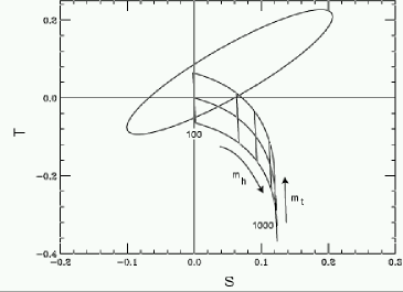
Figure 22: Fit of the precision electroweak data to the Standard Model plus the $S$, $T$ parameters described in the text (from Peskin and Wells [243]). The ellipse is the fit; the warped grid is the Standard Model predictions. The figure uses only the values of the three best electroweak observables, $M_{W}$, the value of the weak mixing angle which appears in $Z^{0}$ decay asymmetries, and $\Gamma_{\ell}$ (the leptonic width of the $Z^{0}$. All data is combined in a plot of M. Swartz at the 1999 Lepton-Photon Conference [244]).

While Figure 22 favors a low mass Higgs boson, $M_{h}\mathrel{\vbox{\hbox{$<$}\nointerlineskip\hbox{$\sim$}}}200$ GeV, we emphasize that this does not imply that a low mass Higgs boson is compelled to exist. The warped grid is only a perturbative Higgs boson mass plot. If the Higgs boson is indeed heavy, then there must be associated new strong dynamics, and there will occur additional new physics contributing to $S$ and $T$. One cannot, therefore, rely upon the perturbative mass plot overlay for large Higgs boson masses. An example of a model in which the Higgs boson mass is $\sim 1$ TeV, but is naturally consistent with the $S$-$T$ error ellipse is the Top Quark Seesaw theory [245] [246], described in Section 4.4.

In general, however, one may still use the $S-T$ error ellipse itself to assess the agreement of a given theory with the data. The contributions to $S$ from classic Technicolor are large and positive. As seen in Appendix A, the contribution of a single weak isodoublet with $N_{T}$ Technicolors is, in a QCD-like dynamics:

$$\Delta S\approx\frac{N_{T}}{6\pi}$$ (3.105)

since the techniquarks are massless and have degenerate constituent quark masses. Thus, with $N_{T}=4$ the minimal model with a single weak isodoublet will give a correction to the $S=T=0$ reference point of $\Delta S=+0.2$ and corresponds roughly to the case of a $\sim 1$ TeV Higgs boson mass with $\Delta T\sim-0.3$. The Farhi-Susskind model has a full generation of $3$ colors each of techniquarks and a “fourth color” of leptons, and thus yields $\Delta S\sim 0.8$ with $\Delta T\sim-0.3$, and would appear to be ruled out. In the minimal model we might be able to pull ourselves from the point $(0.2,-0.3)$ back into the experimentally favored ellipse by adding a positive contribution to $\Delta T\sim 0.4$ from additional new physics. To return to the ellipse in a Farhi–Susskind–like model would require large negative sources of $S$ as well.

There are possible physical sources of the additional contributions to $S$ and $T$ which are required to make Technicolor consistent with the measured oblique parameters. First, strong dynamics models that address the flavor problem must usually include new higher-dimension operators from physics at higher scales that will affect the oblique parameters; a general analysis has been made by a number of authors [114], [247], [248] [249]. The possible existence of such operators obviates any claim that new dynamical models are ruled out by the $S$-$T$ constraints. Second, the presence of precocious ($\sim$ TeV scale) extra dimensions can play an important role, as recently discussed by Hall and Kolda, [250]. Third, Appelquist and Sannino have shown that the ordering pattern for vector-axial hadronic states in $SU(N)$ vector-like gauge theories close to a conformal transition need not be the same as predicted in QCD-like theories. As a consequence, the $S$-parameter in near-critical technicolor theories can be greatly reduced relative to QCD-like theories [251]. Fourth, specific particle content that can produce overall modest contributions to $S$ and $T$ has been identified. We will mention some of the proposed models shortly.

The contribution to the $S$ parameter from a scalar field with exotic weak charge was considered in [252], [253]. Both the ordinary weak charge under $SU(2)_{L}$ and the charge under custodial $SU(2)_{R}$ play a role. Building on this, Peskin and Wells [243] label a field’s weak isospin $j_{L}$ and assign it the appropriate quantum number $j_{R}$ under the custodial $SU(2)$; they further define: $j_{+}=j_{L}+j_{R}$ and $j_{-}=|j_{L}-j_{R}|$. If one assumes a particle with $J=j_{-}$ has the lowest mass $m$, and all other particles in the multiplet have a common mass $M$, then $\Delta S$ is roughly:

$$\Delta S\sim\frac{\kappa^{\prime}}{3\pi}\log{M^{2}\over m^{2}}\,$$ (3.106)

where:

$$\kappa^{\prime}=-\frac{1}{12}\left[\left({(j_{+}+1)\over(j_{-}+1)}\right)^{2}-1\right]j_{-}(j_{-}+1)(2j_{-}+1)\;.$$ (3.107)

If the particles with the smallest $j_{-}$ are the lightest, then the multiplet can yield negative contributions to $S$. Large values of $|\Delta S|$ can be obtained from multiplets with large weak isospin.

Several avenues for producing small or even negative contributions to $S$ have been discussed in the literature. Models with Majorana neutrino condensates naturally produce negative contributions to $S$ [254], which can in principle compensate large positive contributions. Luty and Sundrum [255] constructed models in which the PNGB’s give negative contributions to $S$. To obtain $\Delta S\simeq-0.1$ from this source, one needs technifermions with $j_{L}=2$ and PNGB’s with masses of order $200$ GeV. More generally, other models may include arbitrary numbers of vectorlike pairs of electroweak charged particles [256] (e.g., both a left-handed and right-handed gauged doublet with $j_{-}=0$ and a Dirac mass coming from other external dynamics) with no cost in $S$. The Top–Seesaw model (Section 4.4) contains additional vectorlike fermions, allowing both $S$ and $T$ to be completely consistent with present data. Likewise, the Kaluzsa-Klein recurrences of ordinary quarks and leptons in extra-dimensional models are vectorlike pairs, and are largely unconstrained by $S$. These examples are discussed in Section 4.6.

It is straightforward to engineer large positive contributions to $\Delta T$ [257]. Particles with masses much larger than $\sim 1$ TeV can contribute to $\Delta T$ if their masses have an up-down flavor asymmetry. The contribution is of order:

$$|\Delta T|\sim\left|\frac{m_{U}^{2}-m_{D}^{2}}{m_{U}^{2}+m_{D}^{2}}\right|\;.$$ (3.108)

$|m_{U}-m_{D}|$ can typically be at of order $100$ GeV. One class of theories that generate this kind of contribution to $\Delta T$ are the Technicolor models in which ETC gauge interactions are replaced by exchange of weak-doublet techni-signlet scalars [258, 259, 260] (see Section 3.5).

The effects of new $Z^{\prime}$ bosons on oblique corrections were studied by many authors (see [243] and references therein). Such particles occur in new strong dynamical models, e.g. as in Topcolor Models. Peskin and Wells investigate the region of parameters for any $Z^{0\prime}$ model in which the shifts due to the $Z^{0\prime}$ compensate those of a heavy Higgs boson. Models with extra dimensions can also exhibit “compensation” between effects of new vector bosons and heavy Higgs bosons. Rizzo and Wells [261] have shown that the 95% C.L. bound on the Higgs boson mass could reach $\sim 300$ to $\sim 500$ GeV for Kaluzsa-Klein masses $M_{KK}$ in the range $\sim 3$ to $\sim 5$ TeV. The coupling of the new sector is typically strong (see Section 4). In this vein, Chankowski et al.  [262] has argued that two-Higgs-doublet models (which can be viewed as effective Lagrangians for composite Higgs models) can be made consistent with the electroweak fits for a Higgs boson mass of $\sim 500$ GeV. Technicolor models can also be made consistent with the precision electroweak fits through these kinds of effects.

A modification of the dynamics of the Technicolor gauge theory itself can produce smaller oblique corrections than naively estimated above. In Walking Technicolor models (Section 3.4), where the Technicolor gauge coupling remains strong between the TC and ETC scales, the theory is intrinsically non-QCD-like and conventional chiral lagrangian, or chiral constituent techniquark estimates are expected to fail. Models of this type would not have a visible Higgs boson and may have no new particles below the first techi-vector mesons, or open techniquark/anti-techniquark threshold: it is difficult to anticipate the spectroscopy in a reliable way since QCD no longer functions as an an analogue computer. There is calculational evidence that dangerous contributions to $\Delta S$ are suppressed by walking. For example, models have been proposed in which the Technicolor enhancements to $\Delta S$ are of order $0.1$ [263], [264], [211]. It is possible to construct a Technicolor model that is consistent with the electroweak data by including enough weak isospin breaking to provide a small positive correction to $\Delta T$. Such a model might have, for example $\Delta S\sim 0.2$, $\Delta T\sim 0.2$.

To summarize, the potential conflicts between models of new strong dynamics and the tight experimental constraints on the size of the oblique electroweak parameters can be averted in several ways. Whether it is particle content, the details of Technicolor dynamics, or the behavior of higher-dimension operators from higher-energy physics which comes to the rescue, it is clear that strong dynamics models are not a priori ruled out. The challenge for model-builders is to produce concrete models that are consistent with the constraints.

3.3 Some Explicit ETC Models

Having introduced the broad theoretical outlines and main experimental challenges of ETC, we now present some explicit models. Our summary emphasizes strategies employed in model-building and does not represent a complete list of all models. This discussion will anticipate some of the ideas of Walking ETC which will be more fully treated in Section 3.4.

3.3.1 Techni-GIM

An essential problem in ETC is to find a way to suppress the flavor changing neutral processes arising from the dangerous $\gamma$ terms. We seek a mechanism to naturally make $\gamma<<\beta$. One possibility is to include a GIM mechanism in the ETC sector (TC-GIM). Here, the aim is to construct a detailed model in which the $\beta$ coefficients are of order unity (to make the fermion masses as large as possible) and a GIM cancellation causes $\gamma<<\beta$, protecting against the unwanted $\Delta S=2$ flavor-changing neutral current interactions. With such a GIM mechanism we might hope to suppress the flavor-changing current-current interactions of eq.(3.101) by a further factor of $\sim\Lambda_{TC}^{2}/\Lambda_{ETC}^{2}$. The lower bound on $\Lambda_{ETC}$ would then be weakened to $\Lambda_{ETC}\mathrel{\vbox{\hbox{$>$}\nointerlineskip\hbox{$\sim$}}}10$ TeV, allowing ETC to generate a generic quark mass as large as $10$ GeV. This would accomodate the $c$ and $b$-quark, but would remain insufficient to produce a top quark mass of order $\Lambda_{TC}$.

A candidate mechanism for achieving a GIM mechanism is to introduce separate ETC gauge groups for each weak hypercharge fermion species [221] [265] [266] [267]. Hence one has a separate ETC gauge group for each the left-handed electroweak doublets, right-handed up-type singlets, and down-type singlets. Weak $SU(2)_{L}$ commutes with all of these gauge groups. The ETC groups are broken in such a way that approximate global symmetries hold, broken only by terms necessary to generate quark and lepton masses, and by gauge symmetries. This implies that the $(\overline{\psi}\psi)^{2}$ operators must be approximately invariant under these global symmetries, and thus, in general no $\Delta S=2$ operators can occur.

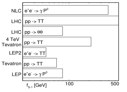
Figure 23: The potential for probing the scale of TC-GIM interactions at present and future colliders (the high-scale models). The most important reaction(s) for each collider is(are) indicated inside the bars (from W. Skiba [174]; $T=P_{3}$, $\theta=P_{8}$ in Skiba’s notation).

This is akin to the Glashow-Weinberg discrete flavor symmetry [268] that was introduced long ago into the multi-Higgs boson extensions of the Standard Model. Indeed the TC-GIM models essentially have Glashow-Weinberg-natural multi-Higgs models as low energy effective Lagrangians. These models are fairly complicated and suffer from the usual limitations on the fermion masses that can be generated in even a Walking TC scheme, e.g., the top quark mass requires an ETC boson mass of order $\Lambda_{TC}$ within this framework. Nonetheless, models which achieve the natural GIM suppression may be possible. The third generation is then clearly special, and part of a sort of inverted hierarchy.

A noticeable feature of these models is the presence of leptoquark PNGB’s, akin to those in the Farhi-Susskind model. Leptoquarks, in most models, typically decay into a quark and a lepton of the same generation. In the TC-GIM models, the leptoquarks can carry the lepton and quark numbers of any generation. This means, for example, that existing limits for leptoquarks decaying only to first-generation or 2nd-generation fermions can be applied directly to TC-GIM models. For example, there are limits on “down-type” first-generation leptoquarks [269] (those decaying to $e+\bar{d}$) and on leptoquarks decaying to 2nd generation fermions[270]. These essentially rule out versions of TC-GIM models in which the dynamical scale is relatively low. The color-octet PNGBs also expected in these models may be detectable at the LHC (see Section 2.3.3).

Skiba has given a detailed survey of signatures of TC-GIM models [174], as summarized in Figure 23. One of most promising TC-GIM signatures at an NLC is pair production of leptoquarks: $e^{+}e^{-}\rightarrow\gamma,\,Z\rightarrow P\bar{P}$, where $P\rightarrow\ell\bar{q}$. Each leptoquark decays into a hadronic jet and an isolated lepton. The events would have two opposite-sign leptons, two hadronic jets and no missing energy, a signature easily disentangled from the backgrounds. It is expected that leptoquarks can be discovered provided that their masses are at least a few GeV below the NLC’s kinematic limit.

3.3.2 Non-Commuting ETC Models

Another approach to ETC model building, which addresses the deviation in $R_{b}$ caused by the $\beta$ terms discussed in 3.1.4, is to drop the assumption that the ETC and weak gauge groups commute [271]. A heavy top quark must then receive its mass from ETC dynamics at low energy scales; if the ETC bosons responsible for $m_{t}$ carry weak charges, we can embed the weak group $SU(2)_{heavy}$ under which $(t,b)_{L}$ is a doublet into an ETC group, or more precisely, a subgroup of ETC which is broken at low scales. To retain small masses, the light quarks and leptons should not be charged under this low-scale ETC group; hence the weak $SU(2)_{light}$ group for the light quarks and leptons must be distinct from $SU(2)_{heavy}$. The resulting symmetry-breaking pattern is:

$$ETC \times SU(2)_{light}\times U(1)^{\prime}\Rightarrow\ \ (f)$$

$$TC\times SU(2)_{heavy} \times SU(2)_{light}\times U(1)_{Y}\Rightarrow\ \ (u)$$

$$TC \times SU(2)_{W}\times U(1)_{Y}\Rightarrow\ \ (v_{0})$$

$$TC \times U(1)_{EM},$$

where $f$, $u$, and $v_{0}=246$ GeV are the VEV’s of the order parameters for the three different symmetry breakings. Note that, since we are interested in the physics associated with top-quark mass generation, only $t_{L}$, $b_{L}$ and $t_{R}$ must transform non-trivially under $ETC$. However, to ensure anomaly cancelation we take both $(t,b)_{L}$ and $(\nu_{\tau},\tau)$ to be doublets under $SU(2)_{heavy}$ and singlets under $SU(2)_{light}$, while all other left-handed ordinary fermions have the opposite $SU(2)$ assignment.

The two simplest possibilities for the $SU(2)_{heavy}\times SU(2)_{light}$ transformation properties of the order parameters that mix and break the extended electroweak gauge groups are:

$$\langle\varphi\rangle\sim(2,1)_{1/2},\ \ \ \ \langle\sigma\rangle\sim(2,2)_{0}~{},\ \ \ \ \ \ \ ``{\rm heavy\ case}"~{},$$ (3.109)

$$\langle\varphi\rangle\sim(1,2)_{1/2},\ \ \ \ \langle\sigma\rangle\sim(2,2)_{0}~{},\ \ \ \ \ \ \ ``{\rm light\ case}"~{}.$$ (3.110)

The order parameter $\langle\varphi\rangle$ breaks $SU(2)_{L}$ while $\langle\sigma\rangle$ mixes $SU(2)_{heavy}$ with $SU(2)_{light}$. In the “heavy” case [271], the technifermion condensation that provides mass for the third generation of quarks and leptons is also responsible for the bulk of electroweak symmetry breaking (as measured by the contribution to the $W$ and $Z$ masses). The “light” case is just the opposite: the physics that provides mass for the third generation does not provide the bulk of electroweak symmetry breaking. While this light case is counter-intuitive (after all, the third generation is the heaviest!), it may in fact provide a resolution to the issue of how large isospin breaking can exist in the fermion mass spectrum (and, hence, the technifermion spectrum) without leaking into the $W$ and $Z$ masses. This is essentially what happens in multiscale models [272, 273] and in Topcolor Assisted Technicolor [274]. Such hierarchies of technifermion masses are also useful for reducing the predicted value of $S$ in Technicolor models[211].

Below the scale of ETC breaking, ETC boson exchange yields four-fermion operators among third-generation quarks and technifermions [271]:

$${\cal L}_{4f}\sim-{1\over f_{ETC}^{2}}\left(\xi\bar{\psi}_{L}\gamma^{\mu}U_{L}+{1\over\xi}\bar{t}_{R}\gamma^{\mu}T_{R}\right)\left(\xi\bar{U}_{L}\gamma_{\mu}\psi_{L}+{1\over\xi}\bar{T}_{R}\gamma_{\mu}t_{R}\right)~{},$$ (3.111)

where $\xi$ is a model-dependent coefficient. When the techniquark condensate forms in the $LR$ cross-terms in these operators we obtain the top quark mass of order eq.(3.98) [172, 173]. In the heavy case the technifermions responsible for giving rise to the third-generation masses also provide the bulk of the $W$ and $Z$ masses, and we expect $F_{T}\approx 125$ GeV (which, for $m_{t}\approx 175$ GeV, implies $f_{ETC}\approx 375$ GeV) [277]. Even in the light case there must also be some $SU(2)_{heavy}$ breaking VEV, in order to give the top quark a mass.

The spectrum of non-commuting ETC models includes an extra set of W and Z bosons which affect weak-interaction physics at accessible energies. Mixing between the two sets of weak gauge bosons alters the $Zff$ couplings. In addition, the one-loop diagram involving exchange of the top-mass-generating boson shifts the coupling of $b_{L}$ to the $Z$ as in eq.(3.98); here, the techniquarks in the loop are up-type, reversing the sign of the final answer. The two physical effects shift $R_{b}$ in opposite directions by similar amounts, leaving $R_{b}$ consistent with experiment [277]. More generally, a recent [278] fit of precision electroweak data to the predictions of the NCETC models yields limits on the masses and couplings of the heavy W and Z bosons. Essentially, if the only modifications to the electroweak observables come from the extra electroweak and ETC bosons of non-commuting ETC, then the heavy W and Z bosons must weigh at least 2.4 TeV in the “light” case and at least 3.3 TeV in the “heavy” case. More general tests of the idea of an extended weak gauge sector at current and future colliders are discussed in Section 3.6.

3.3.3 Tumbling and Triggering

Any successful ETC scheme must provide a dynamical explanation for the breaking of the ETC group to its TC subgroup, as well as for the breaking of the electroweak symmetry. Some interesting ideas fall under the rubrics of “tumbling” and “triggering”.

As mentioned earlier, some ETC models seek to explain the flavor hierarchy of fermion masses by tying it to the sequential breaking of a large ETC gauge group into a succession of subgroups containing, ultimately, the Technicolor interactions. This is called “Tumbling ” [219, 220, 222, 223, 224, 225]. The breaking of the full ETC group down to the Technicolor group proceeds in $n$ steps ${\cal{G}}_{ETC}\rightarrow{\cal{G}}_{1}\rightarrow{\cal{G}}_{2}\rightarrow...{\cal{G}}_{n-1}\rightarrow{\cal{G}}_{TC}$. At each step, the subgroup’s gauge coupling will evolve and become strong, permitting new condensates to form, which further break the theory into the subsequent subgroup. Eventually a low energy theory described by the Technicolor and Standard Model gauge groups is achieved. For discussions of the detailed dynamics of Tumbling, we refer the reader to [279] and more recently [280, 281]. Ref. [282] analyzes all possible tumbling schemes based upon $SU(N)$.

While the tumbling mechanism mentioned above is based on the idea of a group’s breaking itself, some interesting models involve the alternative idea of triggering, in which one gauge theory produces breaking in another. Appelquist et al. [264], [283], [211] explore Technicolor models featuring a non-trivial infrared fixed point of the Technicolor gauge coupling, in which QCD is used to play a triggering role for EWSB. These models, thus, predict a relation between the electroweak scale and the QCD confinement scale. They also predict exotic leptoquarks with masses of $\sim 200$ GeV. Since the oblique corrections are a perennial problem in ETC theories, we mention that isospin splitting and techniquark/technilepton mass splitting in one-family models of this kind have been found reduce the predicted value of the oblique parameter $\Delta S$ to acceptable levels, without giving large contributions to $\Delta T$ [211].

3.3.4 Grand Unification

While the dynamics of pure TC models is tied strongly to the electroweak scale, ETC models inevitably involve physics at higher energy scales. We have already seen that avoiding FCNC in the neutral-$K$ system requires pushing the symmetry-breaking scale of classic ETC models up to at least 1000 TeV. As a result, it is natural for one to ask whether ETC theories can be embedded into a grand-unified gauge theory at still higher energies. A proof-of-principle for the possibility of ETC unification was mentioned earlier: the Farhi-Susskind extension to an SU(56) under which all quarks, leptons, and technifermions transform within one multiplet. We mention some additional unified models in which some of the key theoretical and phenomenological challenges of ETC are also addressed.

Giudice and Raby [241] [242] have considered a unified model that starts with an ETC group of $SO(4)$ with a full standard model family of fermions in the $\bf{4}$ vector representation. This sector of the model is, in spirit, similar to the Farhi-Susskind model with $SO(4)$ replacing $SU(N_{TC})$ and containing the ETC gauge interactions. At the ETC breaking scale $\lambda_{ETC}\sim 10^{3}$ TeV the group $SO(4)$ breaks to $SO(3)$ which is the true gauge Technicolor group. As mentioned above, theories based upon $SO(N)$ groups containing ETC and Technicolor, with fermions in the $\bf{N}$ representation, can avoid flavor-changing neutral current-like interactions ($\gamma$ terms) in the tree approximation. This leads to gauge bosons with masses of order $5$ TeV for third generation,and $\sim 10^{3}$ TeV for first and second, that mediate the ETC interactions. The model exhibits a fixed point in the strong coupling of the Technicolor group, leading the coupling to run slowly (see Section 3.4 on Walking TC) above the TC scale; a key side-effect of walking, the non-calculability of the $S$-parameter, is discussed. The model also invokes four fermion effective operators, and shares features with Top Condensation models (see Section 4).

The main idea is to imbed this ETC theory into a large gauge group such as $SO(18)$ and attempt to achieve a grand unified theory. The breaking chains required for this GUT, curiously, can be generated by Majorana condensates of neutrinos (see e.g. [284]), thus incorporating the Gell-Mann–Ramond–Slansky seesaw mechanism [285] more intimately into the dynamics. Note that neutrino condensates have been invoked elsewhere to break electroweak symmetries, or in concert with fourth generation Farhi-Susskind Technicolor, [286, 284, 287, 288, 289]. The model of Giudice and Raby leaves open the question of breaking the ETC gauge group at $\Lambda_{ETC}$. The exact nature of the Technicolor fixed point (walking) with the additional four-fermion operators is also left unclear.

King and Mannan [290], [57] give a schematic model based upon the three sequential breakings $SO(10)\rightarrow SO(9)\rightarrow SO(8)\rightarrow SO(8)$, where the ETC bosons for $n$th generation of fermions is produced at the $n$th breaking scale. This attempts to explain the generational hierarchy of masses and mixings of the quarks and leptons. The model incorporates grand unification and neutrino masses, but does not address the dynamics behind the sequential breakings as in the Giudice–Raby model.

3.4 Walking Technicolor

3.4.1 Schematic Walking

Extended Technicolor (ETC) has difficulties in producing the observed heavy quark and lepton masses. Even the charm quark is heavy enough to cause problems in building models with sufficiently suppressed flavor-changing neutral-current interactions. In the preceeding section, we surveyed various attempts to deal with this difficulty from a structural point of view. We turn now to an intriguing dynamical possibility which emerges from a closer examination of the full TC strong–dynamics.

Let us consider the TC radiative corrections to the operators from ETC that generate the quark and lepton masses. These operators appear as the “$\beta$” contact terms of eq.(3.87, 3.88) at the scales $\mu\mathrel{\vbox{\hbox{$<$}\nointerlineskip\hbox{$\sim$}}}\Lambda_{ETC}$. Since $\Lambda_{ETC}>>\Lambda_{TC}$, these operators are subject to renormalization effects by TC,

$$\left\langle\bar{Q}Q_{ETC}\right\rangle=\exp\left(\int_{\Lambda_{TC}}^{\Lambda_{ETC}}{d\ln(\mu)}\;\gamma_{m}(\alpha(\mu))\right)\left\langle\bar{Q}Q_{TC}\right\rangle$$ (3.112)

where $\gamma_{m}$ is the operator’s anomalous dimension.

If TC is QCD-like, then the TC coupling constant $\alpha(\mu)$ is asymptotically free, and falls logarithmically as $\alpha(\mu)\propto 1/\ln(\mu)$ above the scale $\Lambda_{TC}$. With the anomalous dimension $\gamma_{m}\propto\alpha(\mu)$ we see that the radiative correction is proportional to $\exp[\gamma_{m}\ln(\ln(\mu)]\sim(\ln(\Lambda_{ETC}/\Lambda_{TC}))^{\gamma_{m}}$. Hence the radiative corrections are power-logarithmic factors, similar to the behavior of QCD radiative corrections to the nonleptonic weak interactions in the Standard Model.

If, however, $\alpha(\mu)$ is approximately constant, i.e., if the TC theory exists approximately at a “conformal fixed point,” $\alpha(\mu)=\alpha^{\star}\neq 0$, where $\beta(\alpha^{\star})=0$, then the radiative correction is converted into a power law, proportional to $\exp[\gamma_{m}(\alpha^{\star})\ln(\mu)]\sim(\Lambda_{ETC}/\Lambda_{TC})^{\gamma_{m}(\alpha^{\star})}$, which is a substantially larger renormalization effect.

Such a theory is not QCD-like, but is an a priori possible behavior of a Yang-Mills gauge theory. This behavior can provide significant amplification to both the $\alpha$ and $\beta$ terms of ETC which involve the technifermion bilinears, but does not alter the dangerous $\gamma$ terms, which involve only the Standard Model fermions. This holds out the possibility of enhancing ETC-generated fermion and PNGB masses without increasing the rate of neutral flavor-changing processes. A TC theory with an approximately constant coupling $\alpha(\mu)=\alpha^{\star}$ in the range $\Lambda_{TC}\mathrel{\vbox{\hbox{$<$}\nointerlineskip\hbox{$\sim$}}}\mu\mathrel{\vbox{\hbox{$<$}\nointerlineskip\hbox{$\sim$}}}\Lambda_{ETC}$ is said to be “Walking Technicolor” (WTC), an idea which was first proposed by Holdom [291]; some early implications were discussed in refs. [292], [293], [294], [295].

3.4.2 Schwinger-Dyson Analysis

As demonstrated by Yamawaki, Bando and Matumuto, [292], and further elaborated by Appelquist, Karabali and Wijewardhana [294], for Walking TC it suffices to have an approximate fixed point, $\beta(\alpha^{\star})<<1$ with $\alpha^{\star}\sim\alpha_{c}$ near $\Lambda_{TC}$, for the relevant scales $\Lambda_{TC}\mathrel{\vbox{\hbox{$<$}\nointerlineskip\hbox{$\sim$}}}\mu\mathrel{\vbox{\hbox{$<$}\nointerlineskip\hbox{$\sim$}}}\Lambda_{ETC}$. Here $\alpha^{\star}$ is near the the critical coupling $\alpha_{c}$ for the formation of chiral condensates. An analysis of the Schwinger-Dyson equations for the mass-gap of the theory [292], [73] then shows that the radiative correction of eq.(3.112) can enhance the techniquark bilinear operator by a factor of order $\Lambda_{ETC}/\Lambda_{TC}$. Essentially, the solution of the Schwinger-Dyson equation with fixed coupling gives large anomalous dimensions $\simeq 1$ near the critical coupling, $\alpha^{*}\sim\alpha_{c}$. This result obtains in the chiral broken phase as well as the symmetric phase, [292] near critical coupling and hence resolves the difficulties in TC (which is supposed to be in the chiral broken phase near $\alpha_{c}$). We recapitulate the argument below.

The Euclideanized Schwinger-Dyson equation for the self-energy of a fermion in Landau gauge is given by [296]:

$$\Sigma(p^{2})=3C_{2}(R)\int\frac{d^{4}k}{(2\pi)^{4}}\frac{\alpha((k-p)^{2})}{(k-p)^{2}}\frac{\Sigma(k^{2})}{Z(k^{2})k^{2}+\Sigma^{2}(k^{2})}$$ (3.113)

Typically we approximate $Z(k^{2})\approx 1$, and linearize the equation by neglecting the $\Sigma^{2}(k^{2})$ denominator term. We assume $\alpha(\mu)\approx\alpha_{c}$ is slowly varying. Two solutions are then found:

$$\Sigma(p^{2})=\Sigma(\mu)\left(\frac{\mu^{2}}{p^{2}}\right)^{b_{\pm}}\qquad b_{\pm}={\textstyle{{1\over{2}}}}(1\pm(1-\alpha(\mu)/\alpha_{c})^{1/2})$$ (3.114)

where the critical coupling constant is $\alpha_{c}=\pi/3C_{2}(R)$, and $C_{2}(R)$ is the quadratic Casimir of the complex technifermion representation $R$ (recall $C_{2}=(N^{2}-1)/2N$ for the fundamental representation).

The normal perturbative anomalous dimension of the $\overline{Q}{Q}$ operator is

$$\gamma_{m}=1-(1-\alpha(\mu)/\alpha_{c})^{1/2}\sim\frac{3C_{2}(R)\alpha(\mu)}{2\pi}$$ (3.115)

Hence, the solution with $b_{-}$ corresponds to the running of a normal mass term of nondynamical origin. The solution with $b_{+}\sim 1$ corresponds to the high momentum tail of a dynamically generated mass having the softer $\sim 1/p^{2}$ behavior at high energies . Note that, at the critical coupling $\alpha(\mu)=\alpha_{c}$, the two solutions coincide, which is believed to be a generic phenomenon, [73], [298], [299]. Moreover, if we suppose that $\alpha(\mu)=\alpha^{*}>\alpha_{c}$ for $0\leq\mu\leq\Lambda^{*}$, then we find that a true dynamical symmetry breaking solution exists where:

$$\Sigma(0)\sim\Lambda^{*}\exp\left(-\pi/\sqrt{\frac{\alpha^{*}}{\alpha_{c}}-1}\right)$$ (3.116)

In the energy range $\Lambda_{TC}\leq\mu\leq\Lambda_{ETC}$, the large value of $\alpha(\mu)\approx\alpha^{*}$ corresponds to an anomalous dimension of order 1, making the radiative correction factor for the technifermion bilinear (3.112) of order $\Lambda_{ETC}/\Lambda_{TC}$.

What are the implications of Walking Extended TC for the ordinary fermion masses? In classic ETC, we have seen that fermion masses typically scale as $\Lambda_{TC}^{3}/\Lambda_{ETC}^{2}$. Since $\Lambda_{TC}\approx 1$ TeV, the phenomenological constraint on $\Lambda_{ETC}\mathrel{\vbox{\hbox{$>$}\nointerlineskip\hbox{$\sim$}}}100$ TeV implies $m_{q,\ell}\mathrel{\vbox{\hbox{$<$}\nointerlineskip\hbox{$\sim$}}}100$ MeV. Walking ETC brings a large renormalization enhancement of the techniquark bilinear by a factor of order $\sim\Lambda_{ETC}/\Lambda_{TC}$, so that we now have [292]:

$$m_{q,\ell}\sim\Lambda_{TC}^{2}/\Lambda_{ETC}\sim 1\;\makebox{GeV}\ ,$$ (3.117)

which is large enough to accomodate the strange and charm quarks, and the $\tau$ lepton. This is born out by more detailed studies which include the full ETC boson exchange in the gap equations [291], [300], [292], [293] [294], [295] [301].

On the other hand, this is barely large enough to accomodate the bottom quark and, certainly not the top quark masses. Consider that, if TC has QCD-like dynamics, the value of $\Lambda_{ETC}$ required to fit the top mass is given by (see [54]):

$$\Lambda_{ETC}\sim 1\;\makebox{TeV}\;\left(\frac{175\makebox{GeV}}{m_{t}}\right)^{1/2}\,.$$ (3.118)

The measured value of the top quark mass therefore implies $\Lambda_{ETC}\sim\Lambda_{TC}$. This leaves too little “distance” between energy scales for walking to make a difference [303]. It therefore appears that ETC alone, even in the presence of walking, can only contribute a fraction of the observed $m_{t}$. We will address alternative mechanisms for producing the masses of the $t$ and $b$ quarks in Section 4. Some of these include new strong gauge dynamics peculiar to the third generation, while others invoke instantons [304] [305].

What is the origin of the small $\beta$ function and what other effects may arise as a consequence? Consider the one-loop $\beta$ function of an $SU(N)_{TC}$ gauge theory with $N_{f}$ techniquarks in the fundamental $N_{TC}$ representation:

$$\beta_{TC}=-\frac{g_{TC}^{3}}{16\pi^{2}}\left(\frac{11}{3}N_{TC}-\frac{8}{3}N_{f}\right)+\cdots$$ (3.119)

Clearly, for $\alpha_{TC}(\mu)=g_{TC}^{2}/4\pi$ to walk requires having many technifermions active between the scales $\Lambda_{TC}$ and $\Lambda_{ETC}$. These need not all be electroweak doublets, e.g., they may be singlets or vectorlike doublets with respect to $SU(2)_{L}$, which can help suppress contributions to $S$. Higher tensor representations of the $SU(N_{TC})$ gauge group are also possible [166]. In general, after the ETC breaking, the fermions in the lower energy theory fall into subsets carrying [i] only (TC); [ii] (TC)$\times$(color); [iii] (TC)$\times$(flavor), and so on, including both the fundamental and higher representations of TC. The technifermions in different representations may condense at different scales, as will be discussed in the next section.

Whether walking is caused by the presence of many technifermions in the fundamental TC representation or technifermions in higher TC representations, the chiral symmetry-breaking sector is enlarged relative to that of minimal TC models. As a result, one expects a proliferation of technipions and small technipion decay constants $F_{T}\ll v_{0}$. At first glance, it appears that the models will suffer from unacceptably large contributions to S (because of the large number of technifermions) and from the presence of many light pseudo-Nambu-Goldstone bosons (PNGBs) which have not been observed. However, the effects of the strong walking-TC dynamics on both issues must be taken into account.

As emphasized by Lane [53], the ingredients that enter conventional QCD-inspired estimations of $S$ are not applicable to a walking ETC theory. Given the altered pattern of resonance masses (possibly a tower of $\rho_{T}$ and $\omega_{T}$ states), the proliferation of flavors, and the presence of fermions in non-fundamental gauge representations [52], it is unclear how to estimate $S$ reliably in a walking model. We note that when estimated naively in a QCD-like TC theory, the S-parameter comes out larger than anticipated, roughly twice the naive result in the fermion bubble approximation. The fermion bubble approximation appears, in spirit, to be closer to the situation in walking ETC. Indeed, existing estimates of $S$ in walking models [306] [307], approach the fermion loop estimate. However, in the absence of compelling evaluations of S in walking gauge theories, S does not provide a decisive test of these models.

In contrast, the effect of walking dynamics on the masses of the PNGB’s is unequivocal: the enhanced condensate raises these masses. Previously we found $m_{P}^{2}\sim\left\langle\bar{Q}Q\right\rangle^{2}/\Lambda_{ETC}^{2}F_{T}^{2}\sim N_{TC}^{2}\Lambda_{TC}^{6}/\Lambda_{ETC}^{2}F_{T}^{2}$, which could be dangerously small. With the enhancements on the pair of bilinear techniquark operators this becomes:

$$m_{P}^{2}\sim N_{TC}^{2}\Lambda_{TC}^{4}/F_{T}^{2}\sim N_{TC}^{2}\Lambda_{TC}^{2}$$ (3.120)

and the PNGB’s are now safely elevated out of harm’s way from current experiments, but left potentially accessible to the Tevatron and LHC.

More generally, Walking TC is actually an illustration of the physics of chiral dynamics in the large $N_{flavor}$ limit. Recent interest in the phase structure of chiral gauge theories has been inspired in part by duality arguments in SUSY theories where there exist exact results for the phase structure of an $SU(N)$ gauge theory with $N_{f}$ flavors (see the review [308]). The presence of infrared fixed points of the gauge coupling appears to be fairly generic in theories with a large number of flavors.

The infrared fixed point of the strong $SU(N)_{TC}$ gauge theory can also arise from the interplay of the first two terms of the $\beta$-function (3.119). The size of the fixed point coupling constant, $\alpha^{*}$, can be controlled by adjusting $N_{f}$ and $N_{TC}$. By judicious choice of $N_{f}\sim N_{TC}$ one can make $\alpha^{*}$ small and a perturbative analysis should be valid. The weak coupling fixed point, truncating $\beta$ on the first two terms, is called the Banks-Zaks fixed point [309]. The ladder-approximation gap equation can be used to probe the chiral breaking transition with fixed point $\alpha^{*}$ [310], which appears to occur for large $N_{f}\mathrel{\vbox{\hbox{$<$}\nointerlineskip\hbox{$\sim$}}}4N\pm 20\%$..

3.5 Multi-Scale and Low-Scale TC

Eichten and Lane [272] [312] have suggested that, if TC dynamically generates the weak scale, there may be distinct sectors of the full theory that contribute components to the full electroweak scale, so that $v_{0}^{2}=v_{1}^{2}+v_{2}^{2}+...$. This general idea is known as “Multi-Scale TC.” The sector of the theory with the smallest $v_{i}$, the “Low-Scale TC” sector, may produce visible phenomenological consequences at the lowest energy scales in current colliders. As we have seen in the previous section, a “Low-Scale” sector is generally expected in a walking TC theory.

Low-Scale TC produces a rich phenomenology, much of which is directly accessible to the Tevatron in Run II or to a low energy LC; a plethora of new states should also be visible at the LHC. Processes of interest in a $f\bar{f}$-collider are then the familiar $f\bar{f}\rightarrow(\rho_{T},\omega_{T})\rightarrow(WW+ZZ,WP_{T}+ZP_{T},P_{T}P_{T})$ as in the Farhi-Susskind model, but transplanted now to the lower scale $v_{i}$. In this section, we will first discuss how the Low-Scale TC idea fits within the general ETC framework and then sketch the phenomenological consequences. Current limits on these theories are discussed in the next section.

The motivation for Low-Scale TC arises directly from the ideas of WTC discussed in the previous section. We have already seen that a WTC coupling is desirable because it offers some remedies for the questions of fermion and PNGB masses. Suppose we follow the lead of Eichten and Lane [272] in constructing a walking model by including technifermions in higher-dimensional TC representations. As the theory evolves downward towards the TC scale, chiral condensates form. However, they do not all form at a single scale: the higher representations will condense out at higher energies since their binding is controlled by the Casimir coefficients, $C_{2}(R)$ of their representations [313]. Moreover, since we have seen how walking dynamics enhances technifermion bilinears, the expected separation of the various condensate scales may be large.

In the most phenomenologically interesting cases of Low-Scale TC, the sector of the theory with the smallest $v_{i}$ includes states light enough to be accessible to current experiments. One caveat is that a very light Low-Scale sector may include charged technipions $P^{\pm}$ with masses less than $m_{top}$. If top quark decays are to remain dominated by the conventional Standard Model channel $t\rightarrow W+b$, as consistent with Tevatron Run I data, it is necessary to suppress a fast $t\rightarrow P_{T}+b$, decay. One possibility is to require that $m_{P}\mathrel{\vbox{\hbox{$>$}\nointerlineskip\hbox{$\sim$}}}160$ GeV [314]. Alternatively, one can decouple the top quark from the Low-Scale sector to suppress the $t\bar{b}P$ vertex [104]. This is generally accomplished by using separate strong top dynamics to generate the top quark (and b-quark) masses and Low-Scale TC for the bulk of the EWSB [274] [315]. A scheme of this type called “Topcolor Assisted TC,” or TC2, and the phenomenological implications of the new strong top dynamics will be discussed in Section 4.2.

In general, the spectroscopy of a Low-Scale TC model can accomodate everything from a minimal model through the Farhi-Susskind structure. The Low-Scale spectrum will, at the very least, include light PNGB’s (technipions) and techni-vector mesons. For example, with $F_{T}\sim 60$ GeV one expects $M_{P_{T}}\sim 100$ GeV and $M_{\rho_{T}}\sim 200$ GeV [52]. The technipions will be resonantly produced via techni-$\rho$ vector meson dominance (VMD) with large rates at the Tevatron, LHC, and a linear collder [316]. The technivector mesons are expected to be, in analogy to the minimal model, an isotriplet, color-singlet $\rho_{T}$, and the isoscalar partner $\omega_{T}$. Isospin is likely to be a good approximate symmetry, so $\rho_{T}$ and $\omega_{T}$ should be approximately degenerate in mass, as is the $I=1$ multiplet of technipions. The enhancement of technipion masses due to walking suggests that the decay channels $\rho_{T}\rightarrow P_{T}P_{T}$ and $\omega_{T}\rightarrow P_{T}P_{T}P_{T}$ are probably closed. Thus, the decay modes $\rho_{T}\rightarrow W_{L}P_{T}$ and $Z_{L}P_{T}$, where $W_{L}$, $Z_{L}$ are longitudinal weak bosons, and $\rho_{T},\omega_{T}\rightarrow\gamma P_{T}$ may dominate. Because technipion couplings to fermions, like those of scalars, are proportional to mass, one expects the most important decay modes to be

$$\begin{array}[]{ll}P_{T}^{0}&\rightarrow b\bar{b}\\ P_{T}^{+}&\rightarrow c\bar{b}\thinspace\thinspace\thinspace{\rm or}\thinspace\thinspace\thinspace c\bar{s},\thinspace\thinspace\tau^{+}\nu_{\tau}\thinspace.\end{array}$$ (3.121)

Heavy-quark jet tagging is, then, important in searches for Low-Scale TC.

Eichten, Lane and Womersley [312] have performed an extensive analysis of the phenomenological signatures of Low-Scale TC at the Tevatron. They present simulations of $\bar{p}p\rightarrow\rho_{T}^{\pm}\rightarrow W^{\pm}_{L}P_{T}^{0}$ and $\omega_{T}\rightarrow\gamma P_{T}^{0}$ for the Tevatron collider with an integrated luminosity of $1\,{\rm fb}^{-1}$. For $M_{\rho_{T}}\simeq 200$ GeV and $M_{P_{T}}\simeq 100\,$ GeV, the cross sections at the Tevatron are expected to be of order a few picobarns. The narrowness of the $\rho_{T}$ and $\omega_{T}$ suggests that appropriate cuts, e.g., on the final state invariant mass, can significantly enhance the signal$/$background ratio. Furthermore, the final states include $b$-quark jets from technipion decay and either a photon or the isolated lepton from weak boson decay. This results in some dramatic signals which stand out well above background when $b$-tagging is required. Cross sections for the LHC are an order of magnitude larger than at the Tevatron, so detection of the light technihadrons should be straightforward there as well.

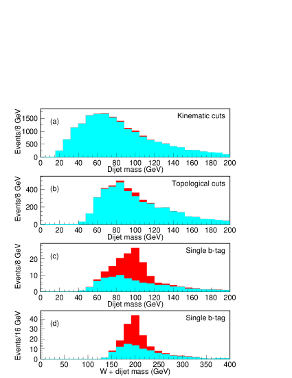
Figure 24: Predicted invariant mass distributions at Tevatron Run II for $\rho_{T}$ signal (black) and $Wjj$ background (grey); vertical scale is events per bin in 1 fb^-1 of integrated luminosity from Ref.([312]). Dijet mass distributions (a) with kinematic selections only, (b) with the addition of topological selections, and (c) with the addition of single $b$-tagging; (d) $W+$dijet invariant mass distribution for the same sample as (c).

More specifically, ref.[312] considers one light isotriplet and isoscalar of color-singlet technihadrons and uses VDM for techni-$\rho$ production and decay to determine the rates for:

$$\begin{array}[]{lll}q\bar{q}^{\prime}&\rightarrow W^{\pm}+\rho_{T}^{\pm}&\rightarrow\thinspace\thinspace W_{L}^{\pm}Z_{L}^{0};\quad W_{L}^{\pm}P_{T}^{0},\thinspace\thinspace P_{T}^{\pm}Z_{L}^{0};\quad P_{T}^{\pm}P_{T}^{0}\\ \\ q\bar{q}&\rightarrow\gamma+Z^{0}+\rho_{T}^{0}&\rightarrow\thinspace\thinspace W_{L}^{+}W_{L}^{-};\quad W_{L}^{\pm}P_{T}^{\mp};\quad P_{T}^{+}P_{T}^{-}\end{array}$$ (3.122)

For $M_{\rho_{T}}\sim 200\,{\rm GeV}>2M_{P_{T}}$ and $M_{P_{T}}\sim 100\,{\rm GeV}$, the dominant processes have cross sections of $1-10$ pb at the Tevatron and $\sim 10-100$  pb at the LHC. The modes with the best signal-to-background are $\rho_{T}\rightarrow W_{L}P_{T}$ or $Z_{L}P_{T}$ and $\rho_{T}\omega_{T}\rightarrow\gamma P_{T}$.

Figure 24(d) shows invariant mass distributions for the $Wjj$ system after kinematic and topological cuts and $b$-tagging have been imposed as discussed in Ref.[312]. A clear peak is visible just below the mass of the $\rho_{T}$, and the peaks in the dijet mass and the $Wjj$ mass are correlated. If the $\rho_{T}$ and $P_{T}$ exist in the mass range favored by the Low-Scale TC models they can be easily found in Run II of the Tevatron. The $\omega_{T}$ is likewise produced in hadron collisions via vector-meson-dominance coupling through $\gamma$ and $Z^{0}$. We expect $\omega_{T}\rightarrow\gamma P_{T}^{0}$, $Z^{0}P_{T}^{0}$ will dominate $\omega_{T}\rightarrow P_{T}P_{T}$.

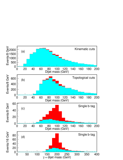
Figure 25: Predicted invariant mass distributions at Tevatron Run II for $\omega_{T}$ signal (black) and $\gamma jj$ background (grey); vertical scale is events per bin in 1 fb^-1 of integrated luminosity. Dijet mass distributions (a) with kinematic selections only, (b) with the addition of topological selections, and (c) with the addition of single $b$-tagging; (d) $\gamma+$dijet invariant mass distribution for the same sample as (c).

Figure 25(a) shows the invariant mass distribution of the two highest-$E_{T}$ jets for signal (black) and background (grey) events, that pass certain kinematic criteria, for an integrated luminosity of $1\,{\rm fb}^{-1}$. The effect of topological cuts is seen in Fig. 25(b). Tagging one $b$-jet significantly improves the signal/background as in Fig. 25(c), and a peak below the $P_{T}$ mass can be seen. Figure 25(d) shows the photon$+$dijet invariant mass after various topological cuts and $b$-tagging are implemented [312].

The ultimate virtue of Low-Scale TC is that the new strong dynamics, presumably the key to other fundamental questions, such as those of fermion masses and flavor physics, would commence at relatively lower accessible energies. As we have seen, Low-Scale TC signatures $\rho_{T}\rightarrow WP_{T}$ and $\omega_{T}\rightarrow\gamma P_{T}$ can be discovered easily in Run II of the Tevatron for production rates as low as a few picobarns. In the next section, we will examine existing experimental constraints on these models.

3.6 Direct Experimental Limits and Constraints on TC

Experiments performed in the past few years have had the large data samples, high energies, and heavy-flavor-tagging capabilities required to begin direct searches for the new phenomena predicted by models of new strong dynamics. We have just examined some of the theoretical implications for preferred channels of Low-Scale TC models. We now summarize the status of experimental limits on the accessible scalar mesons, vector mesons, and gauge bosons, that are generically predicted by these theories. Our focus here is on the direct searches performed largely by the LEP and Tevatron experiments, and we present many of their original exclusion plots. Tables summarizing many of these results may be found in refs. [317, 194]. As appropriate, we will also comment on more indirect searches for new physics via measurements of precision electroweak observables and on the prospects for the LHC and future lepton colliders. For further discussion of technicolor searches at LHC and even higher-energy hadron colliders, see ref. [194].

3.6.1 Searches for Low-Scale Color-singlet Techni–$\rho$’s and Techni–$\omega$’s (and associated Technipions)

In light of the Low-Scale TC model, and the generic phenomenology of TC, it is useful to examine the present-day constraints that exist, mostly from LEP and the Tevatron, on the direct observables, i.e., the masses and production signatures of technivector mesons and techni-$\pi$’s. Note that a number of the searches have taken advantage of the fact that the $\omega_{T}$ of Low-Scale models can be visible in collider experiments [272, 316, 312, 52]. Enhancement of technipion masses by WTC can quench the decay $\omega_{T}\to P_{T}P_{T}P_{T}$, resulting in the dominant mode $\omega_{T}\to\gamma P_{T}$ [272]. Techni-$\omega$ decays to $q\bar{q}$, $\ell^{+}\ell^{-}$ and $\nu\bar{\nu}$ can also be significant, but the decay $\omega_{T}\to ZP_{T}$ is phase-space suppressed.

CDF has published two searches for color-singlet techni-$\rho$’s [318, 319]. One study assumes that the channel $\rho_{T}\to P_{T}P_{T}$ is closed and the other that it is open. If $M_{\rho_{T}}<M_{W}+M_{P_{T}}$ then the techni-$\rho$ (and its isoscalar partner, $\omega_{T}$) decays to pairs of ordinary quarks or leptons. D0 has looked for light $\rho_{T},\omega_{T}$ decaying to $e^{+}e^{-}$ [320]. The LEP collaborations L3 [321], DELPHI [322], and OPAL [323] have released preliminary results on multi-channel searches for light $\rho_{T}$ and $\omega_{T}$.

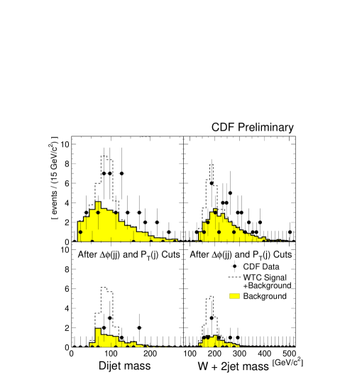
Figure 26: Invariant mass of the dijet system and of the W + 2 jet system (with a leptonically decaying W) in the CDF search for $\rho_{T}\to W^{\pm}P_{T}$ [319]. The points are data; the solid histogram is background; the dashed histogram shows background plus the signal from a walking TC model with $M_{\rho_{T}}=180$ GeV and $M_{P_{T}}=90$ GeV. The topological cuts leading to the lower figures are described in [157].

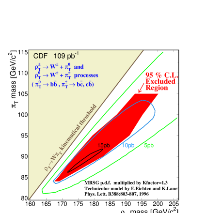
Figure 27: Excluded region for the CDF search for color singlet techni-$\rho$ search in the mode $\rho_{T}\to W^{\pm}P_{T}$. [319]

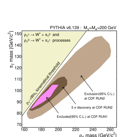
Figure 28: Predicted reach of CDF in Run II for $\rho_{T}\to W\pi_{T}$ assuming $M_{V}=M_{A}=200$ GeV [52] (note the notational variance, $P_{T}=\pi_{T}$).

CDF performed a counting experiment looking for $\rho_{T}\to WP_{T}\to\ell\nu b\bar{b},\ell\nu c\bar{b}$ in 109 pb^-1 of Run I data [318, 319]. They selected candidate lepton plus two-jet events with at least one jet $b$-tagged. The presence of peaks in the $M_{b,jet}$ and $M_{W,b,jet}$ distributions would signal the presence of the $P_{T}$ and $\rho_{T}$, respectively, as indicated in figure 26. No deviation from Standard Model expectations was observed. CDF therefore set upper limits on the techni-$\rho$ production cross-section for specific pair of techni-$\rho$ and technipion masses as indicated in Figure 27. In Run II, with a larger data sample and a doubled signal efficiency, CDF expects to explore a significantly larger range of $\rho_{T}$ masses using the same selection criteria, as indicated in Figure 28.

CDF also searched [318, 319] for technipions in the shape of the two $b$-jet mass distribution in $\ell+2$-jet and $4$-jet events, using 91 pb^-1 of Run I data. The former topologies arise as described above; the latter can result from either $\rho_{T}\to WP_{T}$ or $\rho_{T}\to P_{T}P_{T}$ where the technipions decay to heavy flavors and the $W$ decays hadronically. CDF notes that the upper limits ($\sim 100$ pb) this search sets on production of $\sim 200$ GeV techni-$\rho$ decaying to $\sim 100$ GeV technipions provides no immediate improvement in the constraints on TC models. Run II should provide significantly improved sensitivity to these modes.

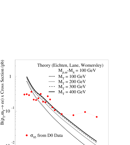
Figure 29: Excluded regions for the D0 search for $\rho_{T},\omega_{T}\to e^{+}e^{-}$ [324].

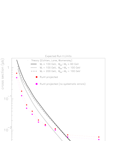
Figure 30: Projected reach of the D0 detector in Tevatron Run IIa for $\rho_{T},\omega_{T}\to e^{+}e^{-}$ [52].

D0 has looked for the light $\rho_{T}$ and $\omega_{T}$ in WTC in which the vector mesons are unable to decay to $W+P_{T}$ [320, 324]. To study the decays $\rho_{T},\omega_{T}\to e^{+}e^{-}$, they selected events with two isolated high-$E_{T}$ electrons, one required to be central, from $\sim 120$ pb^-1 of Run I data. No excess above expected backgrounds was seen. For a model with $N_{TC}=4$, techniquark electric charges of $Q_{D}=Q_{U}-1=-1/3$ and $M_{T}=100$ GeV (this mass parameter is the Low-Scale TC scale, of order the weak interaction scale) [312], $\rho_{T}$ and $\omega_{T}$ mesons with masses below $200$ GeV were ruled out at 95% c.l. provided that $M_{\rho_{T}}-M_{P_{T}}<M_{W}$ (see Figure 29). Projected improvements in the reach of this search in Run II are shown in Figure 30.

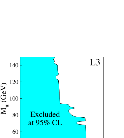
Figure 31: The $M_{\rho_{T}}-M_{P_{T}}$ region excluded by L3 at 95%c.l. [321].

L3 used $176.4$ pb^-1 of data collected at an average center of mass energy of $188.6$ GeV to search for color-singlet $\rho_{T}$. [321]. The search took into account the four major techni-$\rho$ decay modes

$$\rho_{T}\to W_{L}W_{L},W_{L}P_{T},P_{T}P_{T},\gamma P^{(^{\prime})}_{T}$$ (3.123)

for the following range of techni-$\rho$ and technipion masses

$$50\;GeV<M_{P_{T}}<150\;GeV\ \ \ \ \ \ \ \ \ \ 150\;GeV<M_{\rho_{T}}<250\;GeV$$ (3.124)

In the $WW$ decay channel, all decay modes of the W bosons are included. The result is that an upper limit of 0.47 pb was set at 95% c.l. on the possible increase of the $e^{+}e^{-}\to WW$ cross-section due to contributions from TC.

In other decay channels, the technipions decay predominantly to $b\bar{b}$ or $b\bar{c}$ (the calculated branching ratios ranged from 50% to 90%) no statistically significant excess of techni-$\rho$-like events was observed. L3 found the following approximate mass ranges for technipions and techni-$\rho$’s were excluded at 95% c.l., for $150<M_{\rho_{T}}<200$ GeV, technipion masses $50<M_{P_{T}}<150$ GeV were excluded and for $50<M_{P_{T}}<80$ GeV, techni-$\rho$ masses $150<M_{\rho_{T}}<$ 230 GeV were excluded. Figure 31 shows the boundaries of the excluded region.

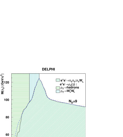
Figure 32: $M_{\rho_{T}}-M_{P_{T}}$ region excluded by DELPHI at 95%c.l. [325]

The DELPHI collaboration searched for technipion production in the final states $W_{L}P_{T}$ and $P_{T}P_{T}$ in four-jet final states [325]. No significant contribution of technipion production was observed, either in the total rate, or in the $M_{jj}$ distribution. DELPHI thus excludes at 95% c.l. technipions of mass between $70$ and $130$ GeV when the techni-$\rho$ mass is between $120$ and $200$ GeV. For heavier $M_{\rho_{T}}$, the range of excluded technipion masses shrinks, as shown in Figure 32, e.g., for $M_{\rho_{T}}=250$ GeV, $70<M_{P_{T}}<100$ GeV is ruled out.

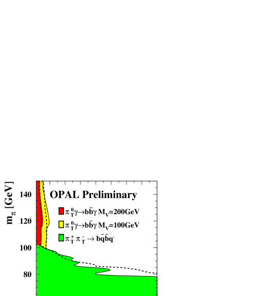
Figure 33: The 95% c.l. excluded region in the ($M_{\rho_{T},\omega_{T}}$) plane from the combination of the $P^{+}_{T}P^{-}_{T}\to b\bar{q}\bar{b}q^{\prime}$ search and the $P^{0}_{T}\gamma\to b\bar{b}\gamma$ search. The dashed lines show the corresponding median expected exclusions for the background only hypothesis. [323]

The OPAL collaboration [323] searched for technihadrons in the channels $e^{+}e^{-}\to\rho_{T},\omega_{T}\to P^{+}_{T}P^{-}_{T}\to b\bar{q}\bar{b}q^{\prime}$ and $e^{+}e^{-}\to\rho_{T},\omega_{T}\to P^{0}\gamma\to b\bar{b}\gamma$ at $\sqrt{s}\approx 200-209$ GeV. No significant excess over SM background was observed in the total number of events or the dijet mass distribution. Cross-section $\times$ branching ratio upper bounds of 60 - 200 fb were set at 95% c.l., depending on the $P^{\pm}+T$ mass. In the search for neutral technipions, events with a pair of b-jets and an energetic isolated photon were chosen. After kinematic and topological cuts, no excess over the SM background was observed. An upper limit of approximately 50 fb (except when the technipion mass is nearly $M_{Z}$) on the cross-section $\times$ branching ratio was established at 95% c.l. The combined results of these searches are shown in Figure 33.

CDF searched for $\omega_{T}\to\gamma P_{T}$, assuming that the $P_{T}\rightarrow b\bar{b}$ [326]. About 200 events with a photon, a $b$-jet and at least one additional jet were selected from $85$ pb^-1 of data. This was found to be consistent with the Standard Model. The distributions of $M_{b,jet}$ and $M_{\gamma,b,jet}-M_{b,jet}$ show no evidence of resonance production. Thus, CDF obtains an upper limit on (cross-section)$\times$(branching ratio), which it compared to the predictions of the TC models of ref. [312]. The range of excluded masses of $P_{T}$ and $\omega_{T}$ are shown in Figure 34 (the exclusion region boundary is ragged because of statistical fluctuations in the data). CDF noted that, if the channels $\omega_{T}\to P_{T}P_{T}P_{T}$ or $\omega_{T}\to ZP_{T}$ were open, the excluded region would be reduced as shown in the Figure [326]. Had their Monte Carlo included $\rho_{T}\to\gamma P_{T}$ and $\rho_{T},\omega_{T}\to\gamma\pi^{\prime}_{T}$, their excluded region would increase.

Figure 34: The 90%, 95% and 99% c.l. exclusion regions for the CDF search for $\omega\to\gamma P_{T}$ [326]. The inset shows the limit on $\sigma\cdot B$ for $M_{P_{T}}=120$ GeV; the circles indicate the limit and the solid line shows the prediction from [312].

Future experiments should provide definitive tests of Low-Scale TC [312]. The cross-section for $\omega_{T}$ production is $\sim 1-10$ pb for Tevatron, and an order of magnitude larger at the LHC. Simulations by the ATLAS collaboration [327] show that the relatively light techni–vector resonances of Low-Scale TC [212] are well within reach at LHC (Figure 35).

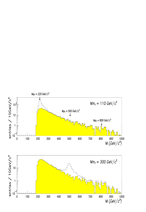
Figure 35: Simulated event and background rates in the ATLAS detector for $\rho_{T}\to W^{\pm}Z\to\ell^{\pm}\nu_{\ell}\ell^{+}\ell^{-}$ for various $M_{\rho_{T}}$ and $M_{P_{T}}$ in low-scale TC models [212]; from Ref. [327].

Experiments at an $e\gamma$ collider have potential to discover and study an $\omega_{T}$ with a mass up to about $\sim 1$ TeV in the processes $e^{-}\gamma\to e^{-}\omega_{T}\to e^{-}\gamma Z,e^{-}W^{+}W^{-}Z$ [328]. As shown in Figure 36, at the stage where only detector acceptance cuts have been applied, the cross-section for an $\omega_{T}$ decaying to $WWZ$ can be of order $\sim 10-100$ fb, and as much as an order of magnitude above background ($\omega_{T}\rightarrow Z\gamma$ is below background). Applying various kinematic cuts, the $\omega_{T}$ could be visible for a range of masses and decay widths. For example, with 200 $fb^{-1}$ collected at $\sqrt{s}=$ 1.5 TeV, an $\omega_{T}$ of width $100$ GeV can be detected at the $3\sigma$ level up to a mass of about $\sim 1.3$ TeV.

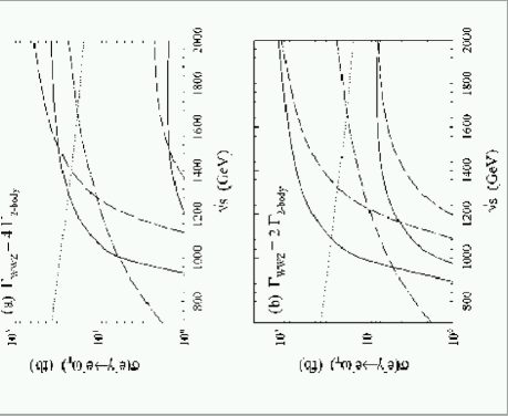
Figure 36: Cross-section vs $e^{+}e^{-}$ CM energy for $e^{-}\gamma\to e^{-}\omega_{T}$ with $\omega_{T}\to WWZ$ and $Z\gamma$ and the SM backgrounds thereto. Solid (long-dashed) lines are for $M_{\omega_{T}}=0.8$ (1.0) TeV. In each case, the upper curve is for $WWZ$ and the lower is for $Z\gamma$. The dash-dot (dotted) line is for the SM $e^{-}WWZ$ ($e^{-}Z\gamma$) background. In (a), $0.25\Gamma_{WWZ}=\Gamma_{Z\gamma}$ = 5 GeV (solid) or 20 GeV (long-dashed); in (b), $0.5\Gamma_{WWZ}=\Gamma_{Z\gamma}$ = 15 GeV (solid) or 40 GeV (long-dashed). (From [328])

3.6.2 Separate Searches for color-singlet $P^{0},P^{0}{}^{\prime}$

$M_{P_{T}^{0^{\prime}}}\leq$	$N_{TC}\sqrt{N_{D}}\leq$
	${P_{T}^{0^{\prime}}}\to gg$	${P_{T}^{0^{\prime}}}\to\bar{b}b$
30 GeV	$28^{(b)}$	$24^{(b)}$
60 GeV	$67^{(b)}$	$70^{(b)}$
80 GeV	$283^{(b)}$	$25^{(a)}$
100 GeV	—	$40^{(a)}$
120 GeV	—	$42^{(a)}$
140 GeV	—	$49^{(a)}$
160 GeV	—	$68^{(a)}$

Table 5: Limits (from ref. [329] on the number of technicolors, $N_{TC}$, and weak doublets of technifermions, $N_{D}$, for hadronically decaying PNGBs in TCSM [212, 213] models as a function of the upper bound on the PNGB mass. The superscripted labels indicate the data used to calculate the limits: (a) means ${\cal A}_{\gamma\gamma P^{a}}$ ; (b) means ${\cal A}_{\gamma ZP^{a}}$.

As discussed in Sections 3.4 and 4, many TC models require a large number $N_{D}$ of weak doublets of technifermions. For a given TC gauge group $SU(N_{TC})$, the number of doublets required to make the gauge coupling $g_{TC}$ “walk” is $N_{D}\approx 10$, as in the models of refs. [315, 330, 331]. Topcolor-Assisted TC models (see Section 4) also tend to require many doublets of technifermions  [212, 315]. One phenomenologically interesting consequence of the large number of doublets is the presence of PNGB states with small technipion decay constants: $F_{T}\approx v_{0}/\sqrt{N_{D}}$. Such states will be lighter, and have generically longer lifetimes.

As outlined in Section 2.3.4, data from LEP can place limits on single production of light neutral PNGB’s from a variety of TC models. One benchmark example is the Lane’s low-scale TC “Straw Man Model” (TCSM) [212, 213], in which the lightest technifermion doublet, composed of technileptons $T_{U}$ and $T_{D}$ can be considered in isolation. The result is two, nearly degenerate neutral mass eigenstates, whose generators are given by $P_{T}^{0}\sim\bar{T}_{U}\gamma_{5}T_{U}-\bar{T}_{D}\gamma_{5}T_{D}$ and $P_{T}^{0}{}^{\prime}\sim\bar{T}_{U}\gamma_{5}T_{U}+\bar{T}_{D}\gamma_{5}T_{D}$. As shown in ref. [329] LEP searches for hadronically-decaying scalars produced in association with a Z or $\gamma$ may be used to place an upper bound on the product $N_{TC}\sqrt{N_{D}}{\cal A}$ (where ${\cal A}$ is the relevant anomaly factor). Inserting the value of ${\cal A}$ appropriate to a particular PNGB yields an upper on $N_{TC}\sqrt{N_{D}}$. Table 5 gives these bounds as a function of PNGB mass for the cases where either 2-gluon or $\bar{b}b$ decays dominate.

Consider the case where $M_{P_{T}^{0}{}^{\prime}}\leq 30$ GeV and $b$-quark decays dominate; the limit $N_{TC}\sqrt{N_{D}}\leq 24$ applies. As a result, for $N_{TC}=(4,6,8,10,12)$ the largest number of electroweak doublets of technifermions allowed by the LEP data is, respectively, $N_{D}=(36,16,9,5,4)$. The results are very similar if the two-gluon decays of the PNGB dominate instead. How do these results accord with the requirements of Walking TC? Requiring the one-loop TC beta function to satisfy $\beta_{TC}\approx 0$, implies that $11N_{TC}/4$ weak doublets of technifermions are needed, according to eq. (3.119). The analysis of ref. [329] thus shows that WTC and a very light $P_{T}^{0}{}^{\prime}$ can coexist only in models with $N_{TC}$ = 4, 6. Similarly, the size of the TC group is restricted to $N_{TC}\leq 6[12]$ if the PNGB mass is 80 GeV [160 GeV]. The results are similar if the 2-loop $\beta$-function is used.

As a second example, we mention the results of ref. [329] for the WTC model of Lane and Ramana [156] whose LEP–II and NLC phenomenology was studied by Lubicz and Santorelli [207]. The model has $N_{D}=9$: one color-triplet of techniquarks ($N_{Q}=1$) and six color-singlets of technileptons ($N_{L}=6$). Of the several neutral PNGBs in this model, the one whose relatively large anomaly factors and small decay constant ($F_{T}\approx 40$ GeV) makes it easiest to produce is $P_{L}^{3}\sim\bar{N}_{\ell}\gamma_{5}N_{\ell}-\bar{E}_{\ell}\gamma_{5}E_{\ell}$ where the subscript implies a sum over technilepton doublets. This PNGB is expected to have a mass in the range $\sim 100-350$ GeV [207]. Depending on the value of the ETC coupling between the PNGB and fermions, the dominant decay of this PNGB may be into a photon pair or $\bar{b}b$. Ref. [329] finds that if the two-photon decays dominate, the PNGB must have a mass in excess of 160 GeV; if the $\bar{b}b$ decay is preferred, the mass range 80 GeV $\leq M_{P}\leq$ 120 GeV is excluded.

3.6.3 Separate searches for color-singlet $P_{T}^{\pm}$

Models with more than the minimal two flavors of new fermions (e.g. TC with more than one weak doublet) typically contain electrically charged PNGB states ($P_{T}^{\pm}$). Experimental limits on charged scalars are often phrased in the language of a two-higgs-doublet model, i.e., in terms of the ratio of the vacuum expectation values of the two doublets ($\tan\beta$) and the mass of the charged scalar ($M_{H}^{+}$).

(i) LEP limits

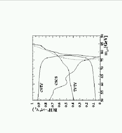
Figure 37: LEP lower bounds on $M_{H^{\pm}}$ as a function of $B(H^{+}\to\tau\nu)$. From [317].

Color-singlet electrically-charged technipions $P_{T}^{\pm}$ with the quantum numbers of the charged scalars in two-higgs-doublet models are directly constrained by the limits on pair-production of $H^{\pm}$ derived from LEP data. When $\tan\beta$ is large, the charged scalars of two-higgs-doublet models decay mostly to $\tau\nu$ ; if $\tan\beta$ is small, light charged scalars decay to $c\bar{s}$, but for $M_{H^{\pm}}$ heavier than about 130 GeV, the channel $H^{+}\rightarrow t\bar{b}\rightarrow Wb\bar{b}$ dominates [332, 333]. The LEP searches assume that $H^{+}\to\tau^{+}\nu_{\tau},c\bar{s}$ (as consistent with the mass range they can probe), and derive limits on the rate of $H^{+}H^{-}$ as a function of the branching ratio $B(H^{+}\to\tau^{+}\nu_{\tau})$. As shown in Figure 37, the lower limit is at least $77$ GeV for any value of the branching ratio.

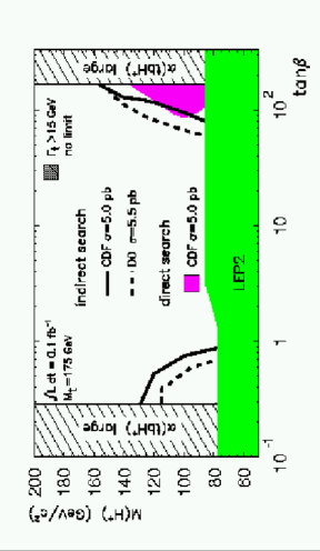
Figure 38: Limits on charged scalar mass as a funciton of $\tan\beta$. The 95% exclusion bounds from CDF and D0 studies of top decays are strong functions of $\tan\beta$. LEP limits from figure 37 are also shown. From [317].

If the mass of the charged scalar is less than $m_{t}-m_{b}$, then the decay $t\to H^{+}b$ can compete with the standard top decay mode $t\to Wb$. Since the $tbH^{\pm}$ coupling can be parameterized in terms of $\tan\beta$ as [334]

$$g_{tbH^{+}}\propto m_{t}\cot\beta(1+\gamma_{5})+m_{b}\tan\beta(1-\gamma_{5})\ ,$$ (3.125)

we see that the additional decay mode for the top is significant for either large or small values of $\tan\beta$. The charged scalar, in turn, decays as $H^{\pm}\to cs$ or $H^{\pm}\to t^{*}b\to Wbb$ if $\tan\beta$ is small and as $H^{\pm}\to\tau\nu_{\tau}$ if $\tan\beta$ is large. In any case, the final state reached through an intermediate $H^{\pm}$ will cause the original $t\bar{t}$ event to fail the usual cuts for the lepton + jets channel. A reduced rate in this channel can therefore signal the presence of a light charged scalar. As shown in Figure 38, D0 and CDF have each set a limit [317] on $M_{H^{\pm}}$ as a function of $\tan\beta$ and $\sigma_{tt}$. In Run II the limits should span a wider range of $\tan\beta$ and reach nearly to the kinematic limit as shown in Figure 39.

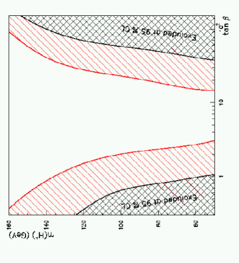
Figure 39: Projected Run II reach of D0 charged scalar search in $t\to H^{\pm}b$ assuming $\sqrt{s}=2$ TeV, $\int{\cal L}dt=2{\rm fb}^{-1}$, and $\sigma(t\bar{t})$ = 7pb.

Limits on the mass and coupling of $P_{T}^{\pm}$ are also implied by the experimental 95% c.l. upper limit $B(b\to s\gamma)<4.5\times 10^{-4}$ obtained by the CLEO Collaboration [335, 336]. Radiative corrections due to the $P_{T}$ tend to increase [337, 338] the branching ratio above the Standard Model prediction of $(3.28\pm 0.33)\times 10^{-4}$ [339, 340], as would be true in a model with an extended Higgs sector. To the extent that this is the only new physics contribution to $b\to s\gamma$, it implies an upper bound of order 300 GeV on the mass of the charged scalar. However, the contributions of other new particles or non-standard gauge couplings can also affect the branching ratio, making the exact limit quite model-dependent. Weaker, and also model-dependent, bounds can also be derived from measurements of $b\to s\gamma$ and $b\to\tau\nu_{\tau}X$ and from $\tau$-lepton decays at LEP [341, 342, 343, 344, 345].

3.6.4 Searches for Low-Scale Color-octet Techni–$\rho$’s (and associated Leptoquark Technipionss)

In models of Walking TC, in which enhancement of the technipion masses prevents the decay $V_{8}\to\bar{P}_{T}P_{T}$ ($V_{8}$ is the color-octet techni–$\rho$), decay to dijets can dominate [291, 316]. The CDF Collaboration has used 87 pb^-1 of Run I data to search for the effects of $V_{8}$’s on the dijet and $b$-tagged dijet invariant mass spectra [346]. No deviations from the Standard Model backgrounds were observed. A narrow $V_{8}$ with mass $350<M_{V_{8}}<440$ GeV is excluded at 95% c.l. using the $b$-tagged distribution, as may be seen in figure 57. The mass range $260<M_{V_{8}}<470$ GeV is ruled out using the untagged sample.

In searches for leptoquark techni-$\pi$’s $P_{3}$, CDF sets $N_{TC}=4$ and allows a relevant parameter, $\Delta M$, to take on the expected value of 50 GeV and the limiting values of 0 and $\infty$. More precisely, $\Delta M$ is the mass difference between $P_{8}$ and $P_{3}$, and enters the calculation of the partial width for $V_{8}\rightarrow\bar{P}_{3}P_{3}$ [156]. CDF reports joint limits on the masses of the $P_{3}$ and $V_{8}$.

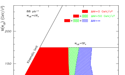
Figure 40: CDF’s 95% c.l. exclusion region for $\rho_{8}\to\bar{P}_{3}P_{3}\to cc\nu_{\tau}\nu_{\tau}$ [347] for several limiting values of $\Delta M=M(P_{8})-M(P_{3})$ which affect the $V_{8}$ decay partial width.

In the first search [348] CDF considered the decay path $P_{3}\to\bar{b}\tau^{-}$. The observed yield was consistent with Standard Model backgrounds (dominated by $Z\to\tau\tau$ plus jets, diboson, and $\bar{t}t$ production). CDF was able to exclude techni–$\pi$ masses up to ($M_{V_{8}}/2$) for $V_{8}$ masses up to about $\sim 450$ $(500,620)$ GeV assuming $\Delta M=0$ $(50,\infty)$, as illustrated in Figure 41. This extends a continuum leptoquark analysis [349] which had previously set the limit $M_{P_{3}}\geq 99$ GeV.

In a second set of searches [347], CDF considered the decay paths $P_{3}\to c\bar{\nu}_{\tau}$ and $P_{3}\to b\bar{\nu}_{\tau}$. No excess of observed events over Standard Model backgrounds (dominated by W + jets) was found. For $P_{3}$ decaying to charm, CDF rules out (Figure 40) technipion masses up to $m_{t}$ for techni-$\rho$ masses up to about $\sim 450$, $(500,650)$ GeV assuming $\Delta M=0$, $(50,\infty)$; heavier $P_{3}$ would decay to $t\nu_{\tau}$. The lower bound from the continuum search in this channel is $M_{P_{3}}\geq 122GeV$ at 95% c.l. For $P_{3}$ decaying to $b\bar{\nu}_{\tau}$, CDF’s continuum search set the 95% lower bound $M_{P_{3}}\geq 149GeV$ and the technipion search excludes $M_{P_{3}}$ up to the kinematic limit ($M_{V_{8}}/2$) for techni-$V_{8}$ masses up to about $\sim 600$ (650, 700) GeV assuming $\Delta M=0$ (50, $\infty$), as shown in Figure 41.

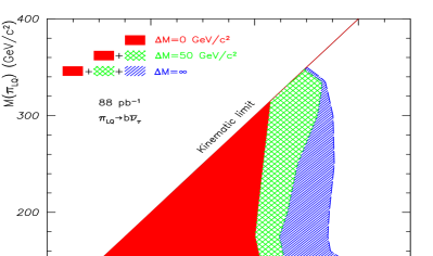
Figure 41: CDF’s 95% c.l. exclusion region for $V_{8}\to P_{3}P_{3}\to bb\nu_{\tau}\nu_{\tau}$ [347] for several values of $\Delta M=M(P_{8})-M(P_{3})$.

Leptoquarks typically decay into a quark and a lepton of the same generation. In the TC-GIM models, the $P_{3}$’s carry lepton and quark numbers of any generation. A leptoquark decaying into an $e$ and $d$–quark has the signature of a “first generation leptoquark.” The first generation leptoquarks decays into $e+\bar{d}$ with branching ratio $\epsilon$, or into a $\nu+\bar{u}$ with branching ratio $1-\epsilon$, and experimental limits are sensitive to the unknown ratio $\epsilon$. In TC-GIM models we have down-type leptoquarks with $\epsilon=1$, and distinct up-types have $\epsilon=0$. We note that the D0 Collaboration  [269] has excluded down-type leptoquarks up to $\sim 130$ GeV, while second generation leptoquarks are excluded by CDF up to $\sim 133$ GeV [270]. This essentially rules out low energy scale versions of the TC-GIM models.

Searches for color-octet technipions will present a greater challenge. It is difficult to pull color-octet technipions, $P_{8}$’s, out of the multijet backgrounds at LHC. However, TC-GIM models can have many different kinds of $P_{8}$’s; if these are nearly degenerate in mass they may give a correspondingly stronger signal. Run II searches for $P_{8}$’s should also consider the rare decay channel decay channel $P_{8}\to g\gamma$ [186, 185]. Although the rate for this mode is down from the two-gluon channel by a factor of about $\sim 100$, a smaller background makes the signal potentially visible, as illustrated in Figure 42. By employing a PYTHIA-level simulation the authors of ref. [185] were able to identify cuts on the transverse momentum and invariant mass of the photon + jet system that significantly enhance the signal relative to the background. They find that the Tevatron Run II can exclude $P_{8}^{0\prime}$ in Low-Scale TC models where $F_{T}$ is reduced to about $\sim 40$ GeV, up to $\sim 350$ GeV, or achieve a $5\sigma$ discovery up to $\sim 270$ GeV. The larger value of $F_{T}$ in the Farhi-Susskind TC model relative to Low-Scale models renders its PNGB invisible in this mode.

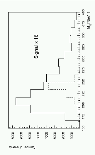
Figure 42: Invariant mass distribution for the $p\bar{p}\to P_{8}^{0\prime}\to g\gamma$ signal (dashed) and background (solid) in multi-scale TC with $M_{P}$ = 250 GeV and $F$ = 40 GeV [185].

3.6.5 Searches for $W^{\prime}$ and $Z^{\prime}$ bosons from $SU(2)\times SU(2)$

As discussed in Section 3.3.2, an integral part of some dynamical theories is an extended $SU(2)_{h}\times SU(2)_{\ell}$ structure for the weak interactions in which the first two generations of fermions are charged under the weaker $SU(2)_{\ell}$ and the third generation feels the stronger $SU(2)_{h}$ gauge force. Examples include the non-commuting extended TC (NCETC) models [271] and the related topflavor models [350, 351, 352, 353]. The low-energy spectrum of the models includes massive W’ and Z’ bosons that couple differently to the third-generation fermions. The more strongly suppressed the new gauge bosons’ couplings to first and second generation fermions, the less effective traditional searches for new electroweak weak bosons become. It is also notable that the new gauge bosons couple, at leading order, only to left-handed fermions (through weak isospin). This section discusses search techniques that exploit the flavor non-universal couplings of the W’ and Z’.

The LEP experiments have studied the possibility that new physics is contributing to electron-positron scattering via four-fermion contact interactions. This allows them to set a lower bound on the mass of a Z’ boson, because at energies well below the mass of the Z’ boson its exchange may be approximated by a four-fermion contact interaction. Their strongest limits on exchange of a Z’ boson arising from extended weak interactions come from processes involving pair production of third-generation fermions: $e^{+}_{L}e^{-}_{L}\to\tau^{+}_{L}\tau^{-}_{L}$ and $e^{+}_{L}e^{-}_{L}\to b_{L}\bar{b}_{L}$. As discussed in ref. [329], the LEP limits on contact-interaction scale $\Lambda$ translate into the following bounds from $\tau\tau$ production

$$M_{Z^{\prime}}=\Lambda\sqrt{\alpha_{em}/4\sin^{2}\theta}\ >\ \left\{\ {365\ {\rm GeV}\ \ \ {\rm ALEPH}}\atop{355\ {\rm GeV}\ \ \ {\rm OPAL}}\right\}\ .$$ (3.126)

and from $bb$ production

$$M_{Z^{\prime}}=\Lambda\sqrt{\alpha_{em}/4\sin^{2}\theta}\ >\ \left\{\ {523\ {\rm GeV}\ \ \ {\rm ALEPH}}\atop{325\ {\rm GeV}\ \ \ {\rm OPAL}}\right\}\ .$$ (3.127)

While these are weaker than the current limits on non-commuting ETC [278] or topflavor [350, 353] Z’ bosons from precision electroweak data (section 3.3.2), they are complementary in the following sense. The limits from a fit to electroweak data assume that the only new relevant physics comes from the extra weak and ETC gauge bosons (or Higgs bosons in topflavor); the contact-interaction limits are lower bounds on the Z’ mass regardless of the other particle content of the theory.

The Fermilab Tevatron experiments have, likewise, searched for new contact interactions contributing to dijet and dilepton production. Because their searches involve only first and second generation fermions, the implied bounds on the mass of a Z’ primarily coupled to the third generation are significantly weaker than those from the LEP data [329].

A W’ boson preferentially coupled to the third generation fermions should be detectable in single top-quark production at Run IIb [354] if its mass is less than about 1-1.5 TeV. The ratio of cross-sections $R_{\sigma}\equiv\sigma(\bar{p}p\to tb)/\sigma(\bar{p}p\to l\nu)$ can be measured (and calculated) to an accuracy [355, 356, 357] of at least $\pm 8\%$. The extra weak gauge bosons present in a non-commuting Extended TC model can change $R_{\sigma}$ in several ways. Mixing of the $W_{h}$ and $W_{\ell}$ bosons alters the light $W$’s couplings to the final state fermions. Exchange of both $W$ and $W^{\prime}$ mass eigenstate bosons contributes to the cross-sections. As a result, a visible increase in $R_{\sigma}$ is predicted.

A direct search for Z’ bosons primarily coupled to the third generation can be made by looking at heavy flavor production at the Tevatron. No searches for these bosons have been made thus far. A recent study [329] (using PYTHIA and a simple model of the D0 detector) indicates that the channel $p\bar{p}\to Z^{\prime}\to\tau\tau\to e\mu\nu\bar{\nu}$ is promising. By requiring large leptonic transverse momenta, low jet multiplicity, and a sufficiently large opening angle between the $e$ and $\mu$, the Run II experiments should be able to overcome the Standard Model backgrounds from $Z^{0}$, $t\bar{t}$ and $WW$ production. A Z’ boson with a mass up to 700 GeV (depending on mixing angle) should be visible, as indicated in figure 43.

Figure 43: Luminosity required to discover SU(2) Z’ bosons preferentially coupled to the third generation [329]. Dashed curves are $3\sigma$ discovery curves for a fixed mass, while solid curves are $5\sigma$ discovery curves. From bottom to top, $3\sigma$ curves are displayed for Z’ masses of 550 GeV, 600 GeV, 650 GeV, and 700 GeV. From bottom to top, $5\sigma$ curves are displayed for Z’ masses of 550 GeV, 600 GeV, and 650 GeV. The horizontal lines indicate luminosity targets for Run II.

Various methods of finding $W^{\prime}$ and $Z^{\prime}$ at the LHC, NLC or FMC have been suggested in the context of topflavor models [350, 351, 352, 353]; in principle these should work equally well for dynamical models. Calculations of expected production rates indicate that a number of processes are worth further study. The presence of a $W^{\prime}$ could boost single top production at the LHC to a rate rivaling that of $t\bar{t}$; the distinctive final state would include a pair of b-jets and a high-$p_{T}$ lepton. Both single-lepton and dilepton production at the LHC could be visibly modified by new weak bosons. A $Z^{\prime}$ boson might visibly alter the rate of di-muon production at an NLC or that of $t\bar{t}$ production at an NLC, FMC or LHC. Since only the left-handed couplings of the top quark would be affected, top angular distributions might also be be altered. Finally, if flavor-changing mixing between second and third-generation leptons were large, production of unlike-sign $\mu\tau$ pairs might be seen. Because the $V_{H}V_{L}V_{L}$ triple gauge boson coupling vanishes to leading order, di-boson production will not reveal the presence of a $W^{\prime}$ or $Z^{\prime}$.

3.7 Supersymmetric and Bosonic Technicolor

3.7.1 Supersymmetry and Technicolor

Shortly after the introduction of Technicolor, Witten described the general aspects of a Supersymmetric Technicolor theory [65], while Dine, Fischler, and Srednicki [66] [67] constructed explicit models. Several interesting possibilities arise when the ideas of Supersymmetry (SUSY) and TC are combined. Notably, it becomes possible to raise the scale of ETC [358], and thus suppress the dangerous $\gamma$ terms. One might even be able to achieve dynamical electroweak symmetry breaking in concert with Supersymmetry breaking. These models are unfashionable at present, relative to the MSSM which guarantees a low-mass Higgs boson accessible to Run IIb or the LHC. Nonetheless, the general idea has some theoretical merit and the models have interesting and accessible phenomenology (including the potential for light fundamental scalars).

In ordinary QCD we know that a chiral condensate, $\left\langle\overline{q}q\right\rangle\neq 0$ is dynamically generated when the gauge coupling becomes strong. In Supersymmetric QCD a quark $q$ possesses a superpartner, denoted $\tilde{q}$, the squark. The supercharge, $Q$, generates a transformation on these fields of the form:

$$\{Q,\tilde{q}^{\dagger}q+{q}^{\dagger}\tilde{q}\}=\overline{q}q$$ (3.128)

Hence, the existence of the fermionic condensate $\left\langle\overline{q}q\right\rangle\neq 0$ implies that:

$$Q|0>\neq 0$$ (3.129)

Whenever $Q$ does not annihilate the vacuum it means that SUSY is broken. The field $\tilde{q}^{\dagger}q+{q}^{\dagger}\tilde{q}$ then becomes a massless Goldstone fermion, a Goldstino. Thus, SUSY breaking and dynamical EWSB can have an intimate connection through fermion condensation.

In addition to the key papers mentioned above, we refer the interested reader to futher works on Supersymmetric Technicolor, refs.[359, 360, 361, 362, 67], and to ref.[363], which discusses the combination of Topcolor with SUSY.

3.7.2 Scalars and Technicolor: Bosonic Technicolor

The key advantage of introducing fundamental scalars into TC is to provide an alternative to ETC. Most of the constraints and problems of ETC can be dismissed by assuming general masses and couplings of the fundamental scalar sector. We thus consider theories in which the additional fields that communicate the TC condensates to the ordinary quarks and leptons are fundamental scalars. We view these scalars as ultimately associated with Supersymmetry, where their masses can be protected by fermionic chiral symmetries [364, 365, 366, 367, 368, 369, 360]. Alternatively, these scalars may, in principle, be bound states arising within a high energy strongly coupled theory [275, 276]. Conceivably, they can also be viewed as relics from extra dimensions, such as Wilson lines (Section 4.6). In what follows, we momentarily disregard the details of the higher-energy physics that enables the scalars to have masses of order the weak scale and consider the key features and phenomenology of TC models with fundamental or effective scalars. We classify the models according to the weak and TC charges of the scalar states.

(i) Weak-doublet Techni-singlet Scalars

We begin by discussing TC models whose spectrum includes one or more weak-doublet TC-singlet scalars. These correspond to a natural low-energy limit of strongly-coupled ETC models [275]. Moreover, the presence of a weak-doublet techni-singlet scalar has a sufficiently large effect on the vacuum alignment of the technifermion condensate to make an $SU(2)$ TC gauge group viable [370].

In the minimal model of this type [258], one adds to the Standard Model gauge and fermion sectors a simple $SU(N)$ TC sector, with two techniflavors that transform as a left-handed doublet $\Upsilon_{L}=(p_{L},m_{L})$ and two right-handed singlets, $p_{R}$ and $m_{R}$, under $SU(2)_{W}$, with weak hypercharge assignments $Y(\Upsilon_{L})=0$, $Y(p_{R})=1/2$, and $Y(m_{R})=-1/2$. The technifermions and ordinary fermions each couple to a weak scalar doublet $\phi=(\phi^{+}\phi^{0})^{T}$ which has the quantum numbers of the Higgs doublet of the Standard Model. Unlike the Standard Model Higgs doublet, $\phi$ has a nontachyonic mass ($M_{\phi}^{2}\geq 0$) and is not the primary source of electroweak symmetry breaking.

The scalar has Yukawa couplings to the technifermions:

$${\cal L}_{\phi T}=\bar{\Upsilon}_{L}\tilde{\phi}\thinspace\lambda_{+}p_{R}\ +\ \bar{\Upsilon}_{L}\phi\thinspace\lambda_{-}m_{R}\ +\ h.c.$$ (3.130)

When the technifermions condense, these couplings cause $\phi$ to acquire an effective VEV, $\langle\phi\rangle=f^{\prime}\approx{4\pi\lambda_{T}f^{3}/M_{\phi}^{2}}$. Because the scalar couples to ordinary fermions as well as technifermions, the ordinary fermions obtain masses from the diagram sketched in Figure 44

$$m_{f}\approx\lambda_{f}h{4\pi f^{3}\over M_{\phi}^{2}}.$$ (3.131)

where $h$ is the scalar coupling to the ordinary fermions. The coupling matrices $\lambda_{f}$ are proportional to the mass matrices $m_{f}$ and drive flavor symmetry breaking. The quark flavor symmetries are broken according to the same pattern as in the Standard Model so that the quarks mix via the usual CKM matrix and the standard GIM mechanism prevails.

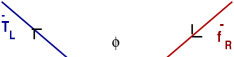
Figure 44: Fermion-technifermion interaction through scalar exchange. This diagram is responsible for fermion mass generation once the technifermions condense.

Both the technipion decay constant and the scalar VEV contribute to the electroweak scale: $f^{2}+f^{\prime 2}=v_{0}^{2}$. The technipions and the isotriplet components of $\phi$ mix. One linear combination becomes the longitudinal component of the $W$ and $Z$; the orthogonal one remains in the low-energy theory as an isotriplet of physical scalars [371]. The coupling of the charged physical scalars to quarks has the same form as in a type-I two-Higgs doublet model [371]. Imposing the requirement that the isoscalar component of $\phi$ have no VEV enables one to eliminate $f$ and $f^{\prime}$ and calculate observables in terms of $M_{\phi}$, $h$ and $\lambda$. This model has been studied in the limits (i) in which $\lambda$ is negligible and one works in terms of ($M_{\phi},h$) [258, 259, 371], and (ii) in which $M_{\phi}$ is negligible and one works in terms of $(\lambda,h)$ [260, 371]. The leading Coleman-Weinberg corrections to the scalar potential have been included in studies of both limits.

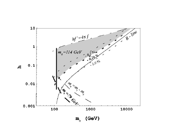
Figure 45: Constraints on technicolor with scalars in limit [i], where the scalar self-coupling is negligible, plotted in the physical basis ($m_{\sigma}$, h). The allowed region of parameter space (shaded) is bounded by the contours $m_{\sigma}=114$ GeV (solid), $R_{b}-R_{b}^{SM}=0.26\%$ (dashes) and $hf^{\prime}=4\pi f$ (dot-dash). Other contours of constant $R_{b}$ are shown for reference. The current bound from searches for charged scalars $m_{\pi^{\pm}_{p}}=79$ GeV is shown (long dashes) along with the reference curve $m_{\pi^{\pm}_{p}}=m_{t}-m_{b}$. The constraint from $B^{0}\bar{B}^{0}$ mixing is labeled “B-line”. [372]

The phenomenology of TC models with weak-doublet scalars has been found to be in agreement with experiment. Models of this kind do not produce unacceptably large contributions to $K^{0}$-$\overline{K^{0}}$ or $B^{0}$-$\overline{B^{0}}$ mixing, nor to the electroweak $S$ and $T$ parameters [258, 259, 260]. In addition, the new scalars in the model can be made heavy enough to evade detection, even in the limit where the scalar doublet is assumed to have a vanishing $SU(2)\times U(1)$ invariant mass [260]. There are negative corrections to $R_{b}$, but they never exceed $-1$% in the regions of parameter space allowed by other constraints; likewise, the rate for $b\to s\gamma$ is less than in the Standard Model, but not so altered as to conflict with experiment [371]. Current bounds on the parameter space of the model [372] are shown in Figures 45 and 46; in creating the plots, the parameters $M_{\phi}$ (limit i) and $\lambda_{\phi}$ (limit ii) have been eliminated in favor of mass of the physical isoscalar state, $m_{\sigma}$.

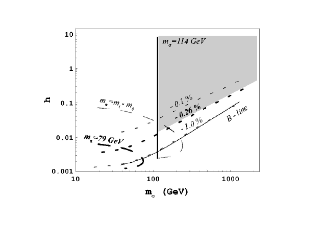
Figure 46: Constraints on technicolor with scalars in limit [ii], where the scalar mass is negligible, plotted in the physical basis ($m_{\sigma}$, h). Curves labeled as in Figure 45. From [372].

Supersymmetrized models with weak-doublet techni-singlet scalars were introduced in refs.[364, 365] and aspects of flavor physics and renormalization group evolution were studied in refs.[366, 367, 368, 369]. The minimal such model [364, 365] contains all the fields of the Minimal Supersymmetric Standard Model (MSSM), a set of $SU(N)_{TC}$ gauge bosons and their superpartners, and color-singlet technifermion superfields transforming under $SU(N)_{TC}\times SU(2)_{W}\times U(1)_{Y}$ as

$$T_{U_{R}}\equiv(N_{TC},1,1/2),\ \ \ T_{D_{R}}\equiv(N_{TC},1,-1/2),\ \ \ T_{L}\equiv(N_{TC},1,0).$$ (3.132)

The superpotential includes $W_{SSM}$ from the MSSM and an additional part $W_{HTC}$ from Yukawa couplings of the two Higgs superfields $H_{U}$ and $H_{D}$ to the technifermion superfields $T$.

$$W_{HTC}=g_{U}H_{U}T_{U_{R}}T_{L}+g_{D}H_{D}T_{D_{R}}T_{L}$$ (3.133)

R-parity is imposed, just as in the MSSM; the technifermions transform like matter.

The Higgs fields have positive squared masses in the perturbative vacuum. The superpotential terms $W_{HTC}$, however, produce terms linear in the Higgs fields in the Lagrangian when the technifermions condense [364, 365]. This causes the Higgs fields to acquire VEV’s:

$$\langle H_{U}\rangle=g_{U}\langle T_{U_{R}}T_{U_{L}}\rangle/m_{H_{U}}^{2}\,,\ \ \ \ \ \langle H_{D}\rangle=g_{D}\langle T_{D_{R}}T_{D_{L}}\rangle/m_{H_{D}}^{2}\,.$$ (3.134)

Thus for $\langle TT\rangle\sim(600\rm{GeV})^{3}$, $g_{U}\sim 1$ and $m_{H_{U}}\sim 1$ TeV, one obtains $\langle H_{U}\rangle\sim 100$ GeV, yielding a realistic top quark mass. If $m_{H_{D}}>m_{H_{U}}$, the VEV of $H_{D}$ will be much smaller than that of $H_{U}$, producing the required top-bottom mass splitting. In variant models with larger technifermion content, $W_{HTC}$ generates technifermion current-algebra masses, yielding masses of order $200$ GeV – $1$ TeV [364, 365] for the technipions in the spectrum.

These supersymmetrized TC models minimize the FCNC problems that usually affect SUSY and TC models [366, 367, 368, 369]. In the minimal version, scalar exchange among quarks and leptons generates no tree-level FCNC. If additional Higgs multiplets are introduced to explain the hierarchy of fermion masses and mixings, tree-level FCNC may be re-introduced; scalar masses of order $\sim 10$ TeV suffice to suppress them. Furthermore, because the lightest Higgs bare mass $m_{H_{U}}$ is of order $\sim 1$ TeV, superpartner masses of order $\sim 1-10$ TeV become natural, reducing the degree of low-energy squark and slepton mass degeneracy required to avoid undue FCNC from loops.

(ii) Weak-singlet Technicolored Scalars

Theories which include weak-singlet technicolored scalars address the intergenerational fermion mass hierarchy more directly. In the early model of ref.[373], exchange of technicolored weak-singlet scalars induces four-fermion interactions between a trio of technifermions and one fermion. Ordinary fermions then mix with technibaryons and become massive. Unfortunately, this model predicts unacceptably large FCNC and tree-level contributions to the $T$ parameter. A more natural account of the mass hierarchy is provided by models [369, 374, 360, 375] in which exchange of technicolored weak-singlet scalars induces four-fermion interactions between pairs of fermions and technifermions. The small CKM elements associated with the third-generation quarks arise because the $t_{L}$ and $b_{L}$ mass eigenstates are automatically aligned. However, because the scalar can couple to both $t_{R}$ and $b_{R}$, the top-bottom mass ratio must be provided by a ratio of Yukawa couplings. We will discuss three models with interesting features in more detail.

Figure 47: (a) Tree-level mass for two generations of fermions due to technifermion condensation. (b) Radiative mass contribution from squark and gluino exchange. Analogous contributions to charged lepton masses arise from exchange of $\xi$ and electroweak gauginos.

A supersymmetric model with technicolored weak-singlet scalars and some interesting mass phenomenology was introduced by Kagan [369]. The gauge group is $SU(N_{TC})\times SU(3)\times SU(2)\times U(1)$; three families of quark and lepton superfields and two sets ($T_{1},T_{2}$) of the color-singlet technifermion superfields as in equation (3.132) are present. The Higgs sector, consists of a vector-like pair of color triplet Higgs fields transforming under $SU(N_{TC})\times SU(3)\times SU(2)\times U(1)$ as $\omega^{c}\equiv(N_{TC},\bar{3},1,-1/6)$ and $\omega\equiv(N_{TC},3,1,1/6)$ and a vector-like pair of color singlet fields $\xi^{c}\equiv(N_{TC},1,1,1/2)$ and $\xi\equiv(N_{TC},1,1,-1/2)$. While only two generations of quarks receive masses at tree-level in this model, gaugino and sfermion exchange enable the first generation fermions to receive radiative masses, as indicated in Figure 47. SUSY breaking masses can be in the $1-10$ TeV range and little or no squark and slepton mass degeneracy is needed. For $N_{TC}=3$, adding a pair of technivector, color, weak- and hypercharge singlet Higgs superfields induces four-technifermion interactions of the form $T_{L}T_{L}T_{U_{R}}T_{D_{R}}$. When technifermion condensation occurs, this generates large current masses for the technifermions, usefully enhancing the masses of the technipions. Phenomenology associated with techniscalar-generated chromomagnetic moments for the quarks and several scenarios for quark mass generation in non-supersymmetric versions of the model are discussed in [369, 376].

Dobrescu has studied a related supersymmetric TC model with only one doublet of technifermions [360]. Only the third generation fermions acquire large masses and the other two generations’ smaller masses are generated radiatively by sfermion and gaugino exchange. The predicted rates of neutral $K$ and $B$ meson mixing, CP violation in $K_{L}$ and $B$ meson decays, and CP asymmetries in $B$ decays or $\Delta S=1$ transitions, are all consistent with experiment.

Dobrescu and Terning [375] have also shown that a TC model with technicolored weak-singlet scalars can produce a negative contribution to the S parameter. This model includes the Standard Model fields, an $SU(N_{TC})$ technicolor gauge group, two flavors of technifermions $\Psi_{R}\equiv(P_{R},N_{R})\equiv(N_{TC},1,2,0)$, $P_{L}\equiv(N_{TC},1,1,1)$, and $N_{L}\equiv(N_{TC},1,1,-1)$ and three technicolored scalars transforming as $\phi\equiv(N_{TC},\bar{3},1,-1/3)$, $\omega_{t}\equiv(N_{TC},\bar{3},1,-7/3)$, and $\omega_{b}\equiv(N_{TC},\bar{3},1,5/3)$. The couplings of the $Z$ boson to the $(t,b)_{L}$ doublet ($\delta g_{L}$) and the $t_{R}$ and $b_{R}$ quarks ($\delta g_{R}^{t},\,\delta g_{R}^{b}$) are found to be shifted by amounts depending on the Yukawa couplings and the scalar masses. The model therefore predicts that the value of the $S$ parameter is reduced from the typical one-doublet techifermion contribution by an amount depending on those couplings:

$$S\approx 0.1N_{TC}-1.02\left(3\delta g_{L}-2\delta g_{R}^{t}+\delta g_{R}^{b}\right)\,.$$ (3.135)

(iii) Weak-doublet Technicolored Scalars

Models incorporating weak-doublet technicolored scalars [370] can explain not only the intergenerational fermion mass heirarchy, but also some elements of the intragenerational mass hierarchies. These models [370] include the Standard Model gauge and fermion sectors together with a minimal TC sector. This takes the form of an asymptotically free $SU(N_{\rm TC})$ gauge group, which becomes strong at a scale of order 1 TeV, and one doublet of technfermions which transform under the $SU(N_{\rm TC})\times SU(3)_{\rm C}\times SU(2)_{\rm W}\times U(1)_{\rm Y}$ gauge group as $\Psi_{L}\equiv(P_{L},N_{L})=(N_{TC},1,2)_{0}$, $P_{R}=(N_{TC},1,1)_{+1}$ and $N_{R}=(N_{TC},1,1)_{-1}$. The large top quark mass is generated by a scalar multiplet, $\chi^{t}$, which transforms under the $SU(N)_{\rm TC}\times SU(3)_{\rm C}\times SU(2)_{\rm W}\times U(1)_{\rm Y}$ gauge group as: $(\overline{N_{\rm TC}},3,2)_{4/3}$. Its Yukawa interactions may be written without loss of generality as

$${\cal L}_{t}=C_{q}\,\overline{q^{3}_{{\scriptscriptstyle L}}}\,\mbox{$N$}_{{\scriptscriptstyle R}}\,\chi^{t}\,+\,C_{t}\,\overline{\Psi}_{\!\!{\scriptscriptstyle L}}\,t_{{\scriptscriptstyle R}}\,i\sigma_{2}\,\chi^{t\dagger}\,+\,{\rm h.c.}~{},$$ (3.136)

where $q_{{\scriptscriptstyle L}}^{3}\equiv(t_{{\scriptscriptstyle L}},b_{{\scriptscriptstyle L}})^{\top}$ is the left-handed weak eigenstate $t-b$ quark doublet, and the Yukawa coupling constants, $C_{q}$ and $C_{t}$, are defined to be positive. Below the scale of technifermion condensation, scalar exchange generates a top quark mass. Because the hypercharge of $\chi^{t}$ allows it to couple to $t_{R}$ but not to $b_{R}$, the model as described gives mass only to the top quark. If other fermion masses arise from physics above the TC scale, it will be natural for the top to be the heaviest fermion. Such physics could be a weak-doublet techni-singlet scalar like that described earlier, or a set of technicolored scalars. In any case, the oblique corrections and Z-pole observables predicted by this class of models are found to be consistent with experiment [370].

4 Top Quark Condensation and Topcolor

The large top quark mass is suggestive of new dynamics, potentially associated with electroweak symmetry breaking. The early papers attempt to identify all of the EWSB with the formation of a top quark condensate, and thus a bound-state Higgs composed of $\bar{t}t$. From this perspective, in contrast to TC, the $W$ and $Z$ and the top quark are the first order massive particles; all other quarks and leptons viewed as a priori massless. We first discuss these pure top condensation scenarios and then review more realistic models incorporating top condensation into a larger dynamical framework.

4.1 Top Quark Condensation in NJL Approximation

4.1.1 The Top Yukawa Quasi-Infrared Fixed Point

Top quark condensation is related to the quasi-infrared fixed point of the top quark Higgs–Yukawa coupling, first discussed by Pendleton and Ross [377] and Hill, [378], [379], with implications for the Higgs boson mass, [380]. At issue are particular properties of the solutions to the Renormalization Group (RG) equations for the top Yukawa coupling constant. The Pendleton-Ross fixed point corresponds to a fixed ratio $g_{t}/g_{QCD}$[377] and is the basis of the idea of “reduction of coupling constants” schemes (e.g., see [381]). It defines a critical trajectory above which $g_{t}$ has a Landau pole, and below which $g_{t}$ is asymptotically free. It predicted $m_{t}\sim 120$ GeV.

On the other hand, the formation of a Higgs bound-state composed of $\bar{t}t$ implies a very large top quark Higgs-Yukawa coupling constant at the scale of the binding interaction $M$. If the top quark Higgs–Yukawa coupling is sufficiently large at a high energy scale $M$ (e.g., if $g_{t}(M)$ is at least of order unity) then one obtains a robust low energy prediction of $m_{t}=g_{t}(m_{t})v_{wk}$, e.g. for $M\sim 10^{15}GeV$ of order $m_{t}\sim 220$ GeV in the Standard Model [378], [379]. (or $m_{t}\sim 200\sin\beta$ GeV, in the MSSM [382]). For arbitrary but sufficiently large initial $g_{t}(M)$ the low energy value of $g_{t}(v_{wk})$ is determined by the RG equations alone. It remains logarithmically sensitive to $M$, but becomes insensitive to the initial $g_{t}(M)$ boundary condition. The term “quasi-infrared fixed point” refers to this solution for the top-Yukawa coupling, and is the RG improved solution of top quark condensation schemes [383].

4.1.2 The NJL Approximation

Nambu discussed the idea of a $\bar{t}t$ condensate in the context of generic chiral dynamics, [384]. This was independently, and more concretely, developed by Miransky, Tanabashi, Yamawaki, et al. [385, 386], who placed the idea firmly in the context of an NJL model and derive the relationship between the top quark mass and electroweak scale through the Pagel’s-Stokar formula. It was subsequently elaborated by Marciano [387], [388], and Bardeen, Hill and Lindner et al. [383]. The latter paper provides a detailed analysis of the scheme with the connection to, and improvement by, the full renormalization group. The Higgs boson is shown to be a “deeply bound state” [389] composed of $\bar{t}t$, where the top and Higgs masses are predicted by the quasi-infrared fixed point [379, 380].

The NJL model for top quark condensation must be considered as an approximation to some supposed new strong dynamics. Indeed, the discussion of models only becomes complete when a concrete proposal for the new dynamics is given, e.g., a new gauge interaction, “Topcolor,” [304] which we discuss in the next section. Technically, the Standard Model can always be rewritten as an NJL model for any fermion, by a sufficiently arbitrary and wide range of choices of higher dimension operators at the composite scale, as emphasized by Hasenfratz et al. [390]. For example, combining certain $d=8$ operators with the $d=6$ NJL interaction, restricting oneself to the fermion bubble approximation, and choosing coefficients for these operators to be absurdly large, of order $\sim 10^{6}$, one can argue that the Higgs is composed of the electron and positron! In doing this, however, one is perversely tuning cancellations of the coupling of composite Higgs boson to its constituents in the infrared, a phenomenon one does not expect in any natural or realistic dynamics.

In Topcolor the additional operators are under control, and one can estimate the coefficients to be small, $\mathrel{\vbox{\hbox{$<$}\nointerlineskip\hbox{$\sim$}}}{\cal{O}}(1)$. Indeed, Topcolor was invented [304] to address the criticism raised in ref.[390]. There are proposals other than Topcolor, based upon strongly coupled $U(1)$ or non–gauge interactions, which also aim to provide a concrete basis for the new strong interaction, see refs. [391], [392], and [393]. As these interactions are not asymptotically free, it is difficult to understand how they become strong in the infrared or unified at high energies. Note that $U(1)$ interactions, moreover, are typically subleading in $N_{c}$ and the NJL model is a large-$N_{c}$ approximation. Topcolor thus has an advantage; we will have a new dynamics such as Topcolor in mind throughout the following discussion.

We can implement the notion of top quark condensation by adapting the Nambu–Jona-Lasinio (NJL) model following ref.[385, 386]. A new fundamental interaction associated with a high energy scale, $M$, involving principally the top quark, is postulated as a four-fermion interaction potential:

$$V\sim-\frac{g^{2}}{M^{2}}(\bar{\psi}^{a}_{L}t_{Ra})_{i}(\bar{t}_{Rb}\psi^{b})^{i}+...$$ (4.137)

where $(a,b)$ are color indices and $(i)$ is an $SU(2)_{L}$ index. This is viewed as a cut-off theory at the scale $M$, (i.e., the interaction presumeably softens due to topgluon exchange above this scale). For any $g^{2}$ this interaction is attractive and will form a bound-state boson, $H\sim\bar{\psi}_{L}t_{R}$. With sufficiently large (supercritical) $g^{2}>g_{c}^{2}$ the interaction will trigger the formation of a low energy condensate, $\left\langle H\right\rangle\sim\left\langle\bar{t}t\right\rangle$. The condensate has the requisite $I=1/2$ and $Y=-1$ quantum numbers of the Standard Model Higgs boson condensate, enabling it to break $SU(2)\times U(1)\rightarrow U(1)$ in the usual way.

The subsequent analysis is a straightforward application of the NJL model, as discussed in Appendix B. For supercritical $g^{2}>g_{c}^{2}$ the theory undergoes spontaneous symmetry breaking. The associated Nambu–Goldstone modes become the longitudinal $W$ and $Z$. In the fermion–loop approximation, one obtains the Pagels-Stokar formula which connects the Nambu–Goldstone boson decay constant, $f_{\pi}=v_{wk}$, to the constituent quark mass, [385, 386, 383]:

$$f_{\pi}^{2}=v^{2}_{wk}=\frac{N_{c}}{16\pi^{2}}m^{2}_{t}(\log\frac{M^{2}}{m_{t}^{2}}+k).$$ (4.138)

Here $m_{t}$ is the top quark mass, which is now the dynamical mass gap of the theory. The constant $k$ is associated with the precise matching onto, and definition of, the high energy theory; it comes from the ellipsis of eq.(4.137), and in Topcolor models $k\mathrel{\vbox{\hbox{$<$}\nointerlineskip\hbox{$\sim$}}}{\cal{O}}(1)$.

Now, if we take the cut–off to be $M\sim 1$ TeV and $k\approx 1$ we predict too large a top quark mass, $m_{t}\sim 600$ GeV. On the other hand, with very large $M\sim 10^{15}$ GeV and $k\approx 1$ we find remarkably that $m_{t}\sim 160$ GeV. Moreover, note that for large $M$ we become systematically less sensitive to $k$.

Unfortunately, in the limit of very large $M>>v_{wk}$ the model is extremely fine-tuned. This is seen from the quadratic running of the (unrenormalized) composite Higgs boson mass in the NJL model, e.g., eq.(B.5):

$$m^{2}_{H}(\mu)=\frac{M^{2}}{g^{2}}-\frac{2N_{c}}{(4\pi)^{2}}(M^{2}-\mu^{2})$$ (4.139)

Taking $\mu\rightarrow v_{wk}$, we see that, in order to have $M>>v_{wk}\sim m_{H}$, the coupling constant of the NJL theory must be extremely fine-tuned:

$$\frac{g^{2}N_{c}}{8\pi^{2}}=1+{\cal{O}}(v_{wk}^{2}/M^{2})$$ (4.140)

This implies extreme proximity of $g^{2}$ to the critical value $g_{c}^{2}=8\pi^{2}/N_{c}$. If $M\sim 10^{15}$ GeV then the coupling must be fine-tuned to within $\sim 1:10^{-30}$ of its critical value.

Critical coupling corresponds to a scale invariant limit of the low energy theory, as in the case of critical coupling in a second order phase transition in condensed matter physics. Choosing a near-critical coupling essentially tunes the hierarchy between the large scale $\sim M$ and the weak scale $v_{weak}$ by having approximate scale invariance over a large “desert.”

In the limit of $M>>v_{wk}$ one can reliably use the renormalization group to improve the predictions for the low-energy top and Higgs masses. The full QCD and Standard Model contributions can be included to arbitrary loop order. For the top quark, the main effect is already seen in the one-loop RG equation:

$$16\pi^{2}\frac{\partial g_{t}}{\partial\ln\mu}=\left(N_{c}+\frac{3}{2}\right)g_{t}^{3}-(N_{c}^{2}-1)g_{t}g_{QCD}^{2}$$ (4.141)

with the “compositeness boundary condition”:

$$\frac{1}{g_{t}^{2}}\rightarrow\frac{N_{c}}{(4\pi)^{2}}\ln(M^{2}/\mu^{2})\qquad\mu\rightarrow M\qquad$$ (4.142)

The boundary condition states that if the Higgs doublet is a pure $\bar{t}t$ bound state, then the Higgs-Yukawa coupling to the top-quark must have a Landau pole at the composite scale $M$. The low energy value of $g_{t}$, as given by the solution to eq.(4.141), is the quasi-infrared fixed point, given by the approximate vanishing of the rhs of eq.(4.141). The fixed point is only $\ln(\ln(M))$ sensitive to the UV scale $M$. The low energy quasi-infrared fixed point prediction in the Standard Model of $m_{t}\approx 220$ GeV with $M\sim 10^{15}$ GeV [378, 379] is large in comparison to the observed $m_{t}=176\pm 3$ GeV. The result does, however, depend on the exact structure (e.g., the particle content) of the high energy theory, and one comes sufficiently close to the physical top mass that perhaps new dynamics can be introduced into the Standard Model to fix the prediction.

In the MSSM, for example, one obtains $m_{t}\sim 200\sin\beta$ GeV, which determines a predicted $\tan\beta$ when compared to the experimental $m_{t}$ [382], [394]. Top quark condensation has been adapted to supersymmetric models [395], but a problem arises. Essentially, the nonrenormalization of the superpotential implies that the effective bound state Higgs mass does not run quadratically; it runs only logarithmically owing to the Kahler potential, or kinetic term, renormalization effects. Hence, the requisite new strong interaction scale $M$ must be of order $v_{weak}$, and cannot be placed in any sensible way at $\sim M_{GUT}$. This may be acceptable in the context of top-seesaw models (Section 4.4), but the general viability of Supersymmetry in these schemes has not been examined. While the quasi-infrared fixed point does play an important role in the MSSM [382], [394], it appears that the naive compositeness interpretation is difficult to maintain in SUSY.

There have been many applications of these ideas to other specific schemes; we mention a few variants here. M. Luty demonstrated how to produce multi-Higgs boson models in the context of top and bottom condensation [396] (see also [397], [398]). The problem of generating the masses of all third generation fermions has been attacked in this context by various authors [399], [400].

Yet another application of these ideas is to the neutrino spectrum, and the formation of neutrino condensates; Hill, Luty and Paschos have considered the dynamical formation of right-handed neutrino Majorana condensates and the see-saw mechanism, [284] [284] (see also: [288]). Some of these models include additional exotic matter such as a sequential fourth generation or leptoquark bound states [401].

Suzuki has discussed the reinterpretation of the compositeness condition as indicating formation of a composite right-handed top quark [402]. Such composites in the NJL context are necessarily Dirac particles, and the Suzuki model affords an interesting variation on the NJL model in which a composite Dirac fermion arises (this of course happens automatically in the composite SUSY models). For related comprehensive reviews of top condensation which describe other variant schema see: [403], [57] and [404].

The key problem with top condensation models is that either (i) the new dynamics lies at a very high energy scale, and the top mass is predicted, but there is an enormous amount of fine–tuning, or (ii) the new dynamics lies at the TeV scale, hence less fine-tuning, yet the predicted top quark mass is then too large. We turn presently to a discussion of more natural models of class (ii), based upon Topcolor, which can provide remedies for these problems.

4.2 Topcolor

4.2.1 Gauging Top Condensation

Our previous discussion of top condensation noted that the relevant interaction Lagrangian, eq.(4.137), must be viewed as an effective description of a more fundamental theory. Let us presently consider what that theory might be. A key observation is that a Fierz rearrangement of the interaction term leads to [304]:

$$-\frac{g^{2}}{M^{2}}(\bar{\psi}^{a}_{L}t_{Ra})_{i}(\bar{t}_{Rb}\psi^{b})^{i}=\frac{g^{2}}{M^{2}}(\bar{\psi}_{iL}\gamma_{\mu}\frac{\lambda^{A}}{2}\psi^{i}_{L})(\bar{t}_{R}\gamma^{\mu}\frac{\lambda^{A}}{2}t_{R})+O(1/N_{c})$$ (4.143)

where $N_{c}=3$ is the number of colors. This is exactly the form (including the sign) induced by a massive color octet vector boson exchange, and suggests a new gauge theory with certain properties: (i) it must be spontaneously broken at a scale of order $M$; (ii) it must be strongly coupled at the scale $M$ to produce deeply bound composite Higgs bosons and trigger chiral condensates; (iii) it must involve the color degrees of freedom of the top quark, analogous to QCD. The relevant models therefore involve embedding of QCD into some large group $G$ which is sensitive to the flavor structure of the Standard Model [304, 274].

¿From this point of view the embedding of QCD into a minimal $SU(3)_{1}\times SU(3)_{2}$ gauge group at higher energies seems a plausible scenario. The second (weaker) $SU(3)_{2}$ gauge interactions act upon the first and second generation quarks while the first (stronger) $SU(3)_{1}$ interaction acts upon the third generation. This drives the formation of the top condensate $\langle\bar{t}t\rangle=0$. Clearly some additional dynamics is then required to suppress the formation of the $b$-quark consdensate, $\langle\bar{b}b\rangle=0$.

We note that a different class of models based upon a strong $U(1)$ gauge interaction has also been proposed by Bonische, [405], Giudice and Raby, [241], and Lindner and Ross, [392] in which the top quark carries the extra, strong $U(1)$ charge. The desired NJL interaction term of eq.(4.137) occurs, but with a $1/N_{c}$ suppression.

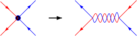
Figure 48: Fierz rearrangement of the attractive Nambu-Jona-Lasinio interaction contains the color current-current interaction to leading order in $1/N_{c}$.

Topcolor Assisted Technicolor (TC2) [304, 274] postulates that the top quark mass is large because it is a combination of (i) a small fundamental component, $\epsilon m_{t}<<m_{t}$ generated by, e.g., ETC or a fundamental Higgs boson, plus (ii) a large dynamical quark mass component, $(1-\epsilon)m_{t}\approx m_{t}$, generated by Topcolor dynamics at the scale $M\sim 1$ TeV, which is coupled preferentially to the third generation. In a pure top condensation model we would have $\epsilon=0$, and we produce the usual three NGB’s that become longitudinal $W^{\pm}_{L}$ and $Z_{L}$. With nonzero $\epsilon$ we are relaxing the requirement that the $\left\langle\bar{t}t\right\rangle$ condensate account for all of the electroweak symmetry breaking.

The ETC component of the top quark mass, the $\epsilon m_{t}$ term, is expected to be $\sim m_{b}$. Hence we assume $\epsilon\mathrel{\vbox{\hbox{$<$}\nointerlineskip\hbox{$\sim$}}}0.1$. Furthermore, the $b$-quark can receive mass contributions from instantons in $SU(3)_{1}$ [406, 304], so that the fundamental EWSB sector (e.g., ETC) needs to provide only a very small, or possibly none of the, fundamental contribution to $m_{b}$. Remarkably the strong CP–$\theta_{1}$ angle in the Topcolor $SU(3)_{1}$ can provide the origin of CKM CP-violation [407].

After all of the dynamical symmetry breaking there are three NGB’s from the TC sector, and three NGB’s from top condensation sector. One linear combination of these, mostly favoring the TC NGB’s, will become the longitudinal $W_{L}^{\pm}$ and $Z_{L}$. The orthogonal linear combination will appear in the spectrum as an isovector multiplet of PNGB’s, $\tilde{\pi}^{a}$. These objects acquire mass as a consequence of the interference between the dynamical and ETC masses of the top quark, i.e., the masses of the $\tilde{\pi}^{a}$ will be proportional to $\epsilon$. We refer to the $\tilde{\pi}^{a}$ as top–pions (note that in the minimal pairing of the $\psi_{L}=(t,b)_{L}$ doublet with the $t_{R}$ singlet there is no singlet top-$\eta^{\prime}$). For $\epsilon\mathrel{\vbox{\hbox{$<$}\nointerlineskip\hbox{$\sim$}}}0.05-0.10$, we will find that the top–pions have masses of order $\sim 200$ GeV. They are phenomenologically forbidden from occuring much below $\sim 165$ GeV [314] due to the absence of the decay mode $t\to\tilde{\pi}{}^{+}+b$.

Because Topcolor and low-scale TC address complementary issues, it is natural to combine these schemes into TC2. [315, 52]. Happily, each half of the model appears to solve many difficulties experienced by the other. For example, since the top quark couples only weakly to ETC in TC2 models, the problem of preventing $t\to P^{+}+b$ in Low-Scale TC is avoided. Moreover, since ETC need not now provide the full top or bottom quark masses, the devastating FCNC constraints on ETC are alleviated (perhaps including some “walking”), producing a viable Technicolor component of the TC2 model. Even the $S$ parameter is likely to be less problematic. We do, however, have to deal with FCNC’s induced by mass mixing of $t$ and $b$ with light quarks, and off-diagonal light PNGB couplings. These can evidently be controlled by systematic choices of fermion mass matrix textures, and the model again appears viable. For discussion of these flavor physics questions, we refer the reader to Section 4.2.4, to [407], which elaborates on the issues raised in [408], and also to [409] and [410].

We mention some variant applications and elaborations of Topcolor. “Bosonic Topcolor,” [411, 412], is based on maintaining the fundamental sector as an elementary Higgs boson, similar in spirit to Bosonic Technicolor (section 3.7.2) and is consistent with current phenomenological constraints. We view Bosonic Topcolor or TC as a useful framework for identifying acceptable model-building directions, with the eventual aim of replacing the fundamental Higgs boson with something dynamical or Supersymmetric [413]. Bosonic Topcolor anticipates a class of models in which SUSY arrives, not near the EWSB scale, but rather closer to the multi-TeV scale. “Topcolor Assisted Supersymmetry,” provides a mechanism for solving the flavor problems in the Sfermion sector [363]. Some authors [414] have argued for a natural origin of Topcolor-like structures in grand-unified models, and models with mirror fermions [415, 416]. Applications to left-right symmetry breaking have also been considered in [287]. Finally, we note that related models involving the idea of a horizontal replication of $SU(2)_{L}\rightarrow G$, where $G$ contains some strong interactions, have been explored under the rubrics of non-commuting extended technicolor [271], (see section 3.3.2) and top-flavor [350, 351, 417]. A potent constraint, often overlooked in these schemes, is the presence of potentially dangerous large instanton effects that violate $B+L$ over some portion of the parameter space of the model [406, 304]).

4.2.2 Gauge Groups and the Tilting Mechanism

In Topcolor models, a new strong dynamics occurs primarily in interactions that involve $\overline{t}t\overline{t}t$, $\overline{t}t\overline{b}b$, and $\overline{b}b\overline{b}b$. The dynamics must cause the top quark to condense, $\left\langle\overline{t}t\right\rangle\neq 0$, while simultaneously suppressing the formation of a large bottom quark condensate, $\left\langle\overline{b}b\right\rangle\approx 0$. This requires “tilting” the vacuum.

Common solutions involve introducing additional strong $U(1)^{\prime}$ interactions that are attractive in the ${\overline{t}t}$ channel and repulsive in the $\left\langle\overline{b}b\right\rangle$ channel [304]. This can take the form of imbedding the weak hypercharge, $U(1)_{Y}\rightarrow U(1)_{Y1}\times U(1)_{Y2}$, since $Y$ has the desired properties. There are then constraints on the running of the strong $U(1)$ couplings and the demands of tilting. Effective field theory analysis of tilting indicates it is not an unreasonable possibility, but may require some fine-tuning at the few percent level [418].

(i) Classic Topcolor

Topcolor with a $U(1)^{\prime}$ tilting mechanism leads to the following gauge group structure at high energies [304]:

$$SU(3)_{1}\times SU(3)_{2}\times U(1)_{Y1}\times U(1)_{Y2}\times SU(2)_{L}\rightarrow SU(3)_{QCD}\times U(1)_{EM}$$ (4.144)

where $SU(3)_{1}\times U(1)_{Y1}$ ($SU(3)_{2}\times U(1)_{Y2}$) couples preferentially to the third (first and second) generations. The $U(1)_{Yi}$ are just rescaled versions of electroweak $U(1)_{Y}$ The fermions are then assigned to $(SU(3)_{1},SU(3)_{2},{Y_{1}},{Y_{2}}$) as follows:

$$(t,b)_{L}\;\; \sim (3,1,{1}/{3},0)\qquad\qquad(t,b)_{R}\sim\left(3,1,({4}/{3},-{2}/{3}),0\right)$$ (4.145)

$$(\nu_{\tau},\tau)_{L} \sim (1,1,-1,0)\qquad\qquad\tau_{R}\sim\left(1,1,-2,0\right)$$

$$(u,d)_{L},\;\;(c,s)_{L} \sim (1,3,0,{1}/{3})\qquad\qquad(u,d)_{R},\;\;(c,s)_{R}\sim\left(1,3,0,({4}/{3},-{2}/{3})\right)$$

$$(\nu,\ell)_{L}\;\;\ell=e,\mu \sim (1,1,0,-1)\qquad\qquad\ell_{R}\sim\left(1,1,0,-2\right)$$

The extended color interactions must be broken to the diagonal subgroup which can be identified with QCD. We assume this is accomplished through an (effective) scalar field:

$$\Phi\sim(3,\bar{3},y,-y)$$ (4.146)

In fact, when $\Phi$ develops a VEV the theory spontaneously breaks down to ordinary QCD $\times U(1)_{Y}$ at a scale assumed to be $\sim 1$ TeV, before Topcolor becomes confining. Nonetheless, the $SU(3)_{1}$ is assumed to be strong enough to form chiral condensates. The vacuum will be tilted by the $U(1)_{Y1}$ couplings which permits the formation of a $\left\langle\overline{t}t\right\rangle$ condensate but disallows the $\left\langle\overline{b}b\right\rangle$ condensate is due to the $U(1)_{Yi}$ couplings.

The symmetry breaking will gives rise to three top-pion states near the top mass scale. If the Topcolor scale is of the order of 1 TeV, the top-pions will have a decay constant, estimated from the Pagel’s-Stokar relation to be $f_{\pi}\approx 60$ GeV, and a strong coupling constant given by, $g_{tb\pi}\approx m_{t}/\sqrt{2}f_{\pi}\approx 2.5$. If $m_{\tilde{\pi}}>m_{t}+m_{b}$, the top-pions may be observable in $\tilde{\pi}^{+}\rightarrow t+\overline{b}$.

Let us define the coupling constants (gauge fields) of $SU(3)_{1}\times SU(3)_{2}$ to be, respectively, $h_{1}$ and $h_{2}$ ($A^{A}_{1\mu}$ and $A^{A}_{2\mu}$) while for $U(1)_{Y1}\times U(1)_{Y2}$ they are respectively ${q}_{1}$ and $q_{2}$, $(B_{1\mu},B_{2\mu})$. The $U(1)_{Yi}$ fermion couplings are then $q_{i}\frac{Yi}{2}$, where $Y1,Y2$ are the charges of the fermions under $U(1)_{Y1},U(1)_{Y2}$ respectively. A techni–condensate or explicit Higgs can break $SU(3)_{1}\times SU(3)_{2}\times U(1)_{Y1}\times U(1)_{Y2}\rightarrow SU(3)_{QCD}\times U(1)_{Y}$ at a scale $M\mathrel{\vbox{\hbox{$>$}\nointerlineskip\hbox{$\sim$}}}240$ GeV, or it can fully break $SU(3)_{1}\times SU(3)_{2}\times U(1)_{Y1}\times U(1)_{Y2}\times SU(2)_{L}\rightarrow SU(3)_{QCD}\times U(1)_{EM}$ at the scale $M_{TC}=240$ GeV. Either scenario typically leaves a residual global symmetry implying a degenerate, massive color octet of “topgluons,” $B_{\mu}^{A}$, and a singlet heavy $Z^{\prime}_{\mu}$. The gluon $A_{\mu}^{A}$ and topgluon $B_{\mu}^{A}$ (the SM $U(1)_{Y}$ field $B_{\mu}$ and the $U(1)^{\prime}$ field $Z^{\prime}_{\mu}$), are then defined by orthogonal rotations with mixing angle $\theta$ ($\theta^{\prime}$):

$$\cot\theta=h_{1}/h_{2};\qquad\qquad\frac{1}{g_{3}^{2}}=\frac{1}{h_{1}^{2}}+\frac{1}{h_{2}^{2}}$$ (4.147)

and:

$$\cot\theta^{\prime}=q_{1}/q_{2};\qquad\qquad\frac{1}{g_{1}^{2}}=\frac{1}{q_{1}^{2}}+\frac{1}{q_{2}^{2}};$$ (4.148)

where $g_{3}$ ($g_{1}$) is the QCD ($U(1)_{Y}$) coupling constant at $M_{TC}$. We demand $\cot\theta\gg 1$ and $\cot\theta^{\prime}\gg 1$ to tilt the strongest interactions and to select the top quark direction for condensation. The masses of the degenerate octet of topgluons and $Z^{\prime}$ are given by $M_{B}\approx g_{3}M/\sin\theta\cos\theta$ $M_{Z^{\prime}}\approx g_{1}M/\sin\theta^{\prime}\cos\theta^{\prime}$. The usual QCD ($U(1)_{Y}$ electroweak) interactions are obtained for any quarks that carry either $SU(3)_{1}$ or $SU(3)_{2}$ triplet quantum numbers (or $U(1)_{Yi}$ charges).

Integrating out the heavy bosons $Z^{\prime}$ and $B$ gives rise to effective low energy four fermion interactions. The effective Topcolor interaction mediated by $B$ is strongest in the third generation and takes the form:

$${\cal{L}}^{\prime}_{TopC} = -\frac{2\pi\kappa}{M_{B}^{2}}\left(\bar{t}\gamma_{\mu}\frac{\lambda^{A}}{2}t+\bar{b}\gamma_{\mu}\frac{\lambda^{A}}{2}b\right)\left(\bar{t}\gamma^{\mu}\frac{\lambda^{A}}{2}t+\bar{b}\gamma^{\mu}\frac{\lambda^{A}}{2}b\right).$$ (4.149)

where:

$$\kappa=\frac{g^{2}_{3}\cot^{2}\theta}{4\pi}$$ (4.150)

This interaction is attractive in the color-singlet $\bar{t}t$ and $\bar{b}b$ channels and invariant under color $SU(3)$ and $SU(2)_{L}\times SU(2)_{R}\times U(1)\times U(1)$ where $SU(2)_{R}$ is the custodial symmetry of the electroweak interactions.

In addition we have the $U(1)_{Y1}$ interaction Lagrangian (which breaks custodial $SU(2)_{R}$):

$${\cal{L}}^{\prime}_{Y1}=-\frac{2\pi\kappa_{1}}{M^{2}_{Z^{\prime}}}\left(\frac{1}{6}\bar{\psi}_{L}\gamma_{\mu}\psi_{L}+\frac{2}{3}\bar{t}_{R}\gamma_{\mu}t_{R}-\frac{1}{3}\bar{b}_{R}\gamma_{\mu}b_{R}-\frac{1}{2}\bar{\ell}_{L}\gamma_{\mu}\ell_{L}-\bar{\tau}_{R}\gamma_{\mu}\tau_{R}\right)^{2}$$ (4.151)

where:

$$\kappa_{1}=\frac{g^{2}_{1}\cot^{2}\theta^{\prime}}{4\pi}\qquad$$ (4.152)

and where $\psi_{L}=(t,b)_{L}$, $\ell_{L}=(\nu_{\tau},\tau)_{L}$ and $\kappa_{1}$ is assumed to be $O(1)$. Note that while too small a value for $\kappa_{1}$ signifies fine-tuning in the model, phenomenological constraints limit how large $\kappa_{1}$ can be.

For sufficiently large $\kappa$, we trigger the formation of a low energy condensate, $\left\langle\overline{t}t+\overline{b}b\right\rangle$, which breaks $SU(2)_{L}\times SU(2)_{R}\times U(1)_{Y}\rightarrow U(1)\times SU(2)_{c}$, where $SU(2)_{c}$ is a global custodial symmetry. The $U(1)_{Y1}$ force is attractive in the ${\overline{t}t}$ channel and repulsive in the ${\overline{b}b}$ channel. We find, in concert, the critical and subcritical values of the combinations:

$$\kappa+\frac{2\,\kappa_{1}}{9N_{c}}>\kappa_{crit};\qquad\kappa_{crit}>\kappa-\frac{\kappa_{1}}{9N_{c}}$$ (4.153)

by using the large-$N_{c}$ NJL (fermion loop) approximation (similar criticality constraints were discussed previously in the NJL model of top condensation of Miransky, Tanabashi, Yamawaki, et al. [385, 386]).

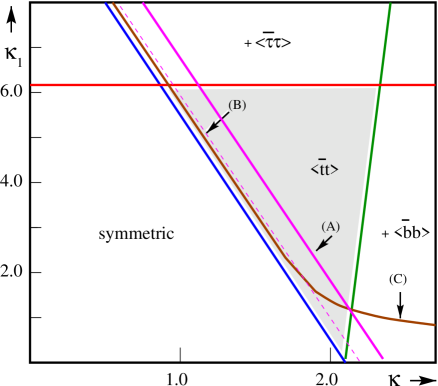
Figure 49: The full phase diagram of the Topcolor model. The top quark alone condenses for values of $\kappa$ and $\kappa_{1}$ corresponding to hatched region. In other regions additional unwanted condensates turn on (for still larger $\kappa_{1}$ a $\left\langle\bar{\tau}b\right\rangle$ condensate forms. (A) $M_{B}=1.0$ TeV; (B) $M_{B}=3.0$ TeV; (C) upper bound from $Z\rightarrow\bar{\tau}\tau$ (figure from [407]).

The phase diagram of the model is shown in Fig.(49) from [407]. The criticality conditions (4.153) define the allowed region in the $\kappa_{1}$–$\kappa$ plane in the form of the two straight solid lines intersecting at $(\kappa_{1}=0,\kappa=\kappa_{crit})$. To the left of these lines lies the symmetric phase, in between them the region where only a $\left\langle\bar{t}t\right\rangle$ condensate forms and to the right of them the phase where both $\left\langle\bar{t}t\right\rangle$ and $\left\langle\bar{b}b\right\rangle$ condensates arise. The horizontal line marks the region above which $\kappa_{1}$ makes the $U(1)_{Y1}$ interaction strong enough to produce a $\left\langle\bar{\tau}\tau\right\rangle$ condensate. This line is meant only as a rough indication, as the fermion-bubble (large-$N_{c}$) approximation, which we have used, fails for leptons. There is an additional constraint from the measurement of $\Gamma(Z\to\tau^{+}\tau^{-})$, confining the allowed region to the one below the solid curve. This curve corresponds to a $2\sigma$ discrepancy between the Topcolor prediction and the measured value of this width. In the allowed region a top condensate alone forms. The constraints favor a strong $SU(3)_{1}$ coupling and allow a range of $U(1)_{Y1}$ couplings.

How does Technicolor know to break Topcolor when the latter triggers chiral condensates? This may involve self-breaking schemes, as considered by Martin [225], [225], [419]. Topcolor interactions may themselves produce the condensate of $\Phi$ as a dynamical boundstate, leading to self-breaking at the Topcolor scale. Other such scenarios require further study.

We can also construct a model with no strong $U(1)$ tilting interaction [304, 274] called “Type II Topcolor.” The model requires additional heavy vectorlike $b$’ quarks, but there is no $Z$’ required for tilting because of the particular gauge charge assignments under Topcolor. These models are intriguing, but have received little attention in the literature, and we refer the interested reader to the original references [304, 274, 407].

(ii) Flavor-Universal Topcolor

The flavor-universal variant of Topcolor [420, 331, 421] is based on the same gauge group as above, but assigns all quarks to be triplets under the strongly-coupled $SU(3)_{1}$ gauge group and singlets of $SU(3)_{2}$. As a result, the heavy color-octet of gauge bosons that results from breaking of the extended color group to its QCD subgroup are “flavor-universal colorons” coupling to all quark flavors with equal strength [420]:

$${\cal L}_{C}=g_{3}\cot\theta(C^{A}\cdot J^{A}_{C})$$ (4.154)

where

$$J_{C}^{\mu\,A}=\sum_{q}\bar{q}\gamma^{\mu}\frac{\lambda^{A}}{2}q$$ (4.155)

The weak and hypercharge assignments of the quarks and leptons are as in Classic Topcolor, so that the properties and couplings of the Z’ boson are unchanged.

Once again, the values of $\kappa_{i}=g_{i}^{2}/4\pi$ are jointly constrained by several different pieces of physics. Above all, the top quark should be the only fermion to condense and acquire a large mass. Applying the gauged NJL analysis [422, 423, 424, 425] to all the Standard Model fermions, one can seek solutions with $\langle\,\bar{t}t\,\rangle\neq 0$ and $\langle\,\bar{f}f\,\rangle=0$ for $f\neq t$. Top condensation occurs provided that [421, 407]

$$\kappa_{3}+{2\over 27}\kappa_{1}\geq{{2\pi}\over 3}-{4\over 3}\alpha_{s}-{4\over 9}\alpha_{Y}$$ (4.156)

where we again take $\kappa_{crit,NJL}\approx 2\pi/3$ [34, 35]. Quarks other than the top quark will not condense provided that additional limits on $\kappa_{1}$ and $\kappa_{3}$ are satisfied. In Classic TC2 models, the limit comes from requiring $\langle\,\bar{b}b\,\rangle=0$, while in flavor-universal TC2 models, an even stronger limit comes from ensuring $\langle\,\bar{c}c\,\rangle=0$ [421]:

$$\kappa_{3}+{2\over 27}{\alpha_{Y}^{2}\over\kappa_{1}}<{{2\pi}\over 3}-{4\over 3}\alpha_{s}-{4\over 9}\alpha_{Y}$$ (4.157)

As shown in Figure (50), the phase diagram of the flavor-universal model includes a region in which only top condensation occurs; the region is similar to that of classic TC2. (see also discussion of phase plane in [424, 425]).

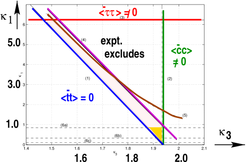
Figure 50: Joint constraints on coloron and Z’ couplings (from [421]). Curves (1), (2), (3) outline the ‘gap triangle’ where only $\langle\,\bar{t}t\,\rangle\neq 0$ in flavor-universal TC2 models; in ordinary TC2 models, the triangle is roughly symmetric about the lowest point. The region above curve (4) is excluded by data on $\Delta\rho_{*}$; the region above curve (5) is excluded by data on $Z\rightarrow\tau^{+}\tau^{-}$. Lines (6a-6c) are upper bounds on $\kappa_{1}$ that hold if the U(1) Landau pole lies one, two, or five orders of magnitude above $\Lambda$. The right-hand bound is steep because it comes from the $\langle\,\bar{c}c\,\rangle=0$ constraint, eq. (4.157).

Several types of physics further constrain the allowed region of the $\kappa_{1}-\kappa_{3}$ plane. As already mentioned for Classic TC2, , mixing between the Z and Z’ bosons alters the predicted value of the Z decay width to tau leptons from the standard model value [407, 421]. The $\rho$ or $T$ parameter is also sensitive both to $Z-Z^{\prime}$ mixing [277] and to single coloron exchange across the top and bottom quark loops of $W$ and $Z$ vacuum polarization diagrams [426, 421]. Finally, if the Landau pole of the strong $U(1)$ interaction is to lie at least an order of magnitude above the symmetry-breaking scale $\Lambda$, then $\kappa_{1}\mathrel{\vbox{\hbox{$<$}\nointerlineskip\hbox{$\sim$}}}1$ [421]. Figure 50 summarizes these constraints on the $\kappa_{1}-\kappa_{3}$ plane for flavor-universal TC2 models. The constraints from $\Delta\rho$ and the Landau pole also apply to the phase diagram in figure 49. In the end, both kinds of Topcolor models are confined to a region of the $\kappa_{1}-\kappa_{3}$ plane in which $\kappa_{1}$ is small and $\kappa_{3}\approx\kappa_{crit,NJL}\approx 2\pi/3$ [421].

4.2.3 Top-pion Masses; Instantons; The b-quark mass

In TC2 a multiplet of PNGB top-pions is naturally present in the spectrum. Top-pion masses are estimated from the loop of Figure(51), which feels both the dynamical mass $\sim m_{t}$ and the explicit mass $\sim\epsilon m_{t}$ [304, 274]. The top–pion decay constant is estimated from the Pagels-Stokar formula; using $M=M_{B}\sim 1.5$ TeV and $m_{t}=175$ GeV, it is $f_{\pi}\approx 60$ GeV. The Lagrangian for the coupling of the top-pions to quarks takes the form:

$$g_{bt\tilde{\pi}}\left[{i}\overline{t}\gamma^{5}t\tilde{\pi}^{0}+\frac{i}{\sqrt{2}}\overline{t}(1-\gamma^{5})b\tilde{\pi}^{+}+\frac{i}{\sqrt{2}}\overline{b}(1+\gamma^{5})t\tilde{\pi}^{-}\right]$$ (4.158)

and the coupling strength is $g_{bt\tilde{\pi}}\approx m_{t}/\sqrt{2}f_{\pi}$ [274]. This Lagrangian, written above in the current basis, will in general contain generational mixing when one passes to the mass-matrix eigenbasis.

Figure 51: The interference of the explicit breaking tewrm $\propto\epsilon$, and the dynamical mass $\sim m_{t}$ yields an estimate of the top-pion mass.

Estimating the induced top-pion mass from the fermion loop yields:

$$m_{\tilde{\pi}}^{2}=\frac{N\epsilon m_{t}^{2}M_{B}^{2}}{8\pi^{2}f_{\pi}^{2}}=\frac{\epsilon M_{B}^{2}}{\log(M_{B}/m_{t})}$$ (4.159)

where the Pagels-Stokar formula is used for $f_{\pi}^{2}$ (with $k=0$) in the last expression. For $\epsilon=(0.03,\;0.1)$, $M_{B}\approx(1.5,\;1.0)$ TeV, and $m_{t}=175$ GeV this predicts $m_{\tilde{\pi}}=(180,\;240)$ GeV. We would expect that $\epsilon$ is subject to large renormaliztion effects and, even a bare value of $\epsilon_{0}\sim 0.005$ consistent with ETC, can produce sizeable $m_{\tilde{\pi}}>m_{t}$.

Charged top-pions as light as $\sim 165$ GeV, would provide a detectable decay mode for top quarks [314]. Burdman has discussed potentially dangerous effects in $Z\rightarrow b\bar{b}$ resulting from low mass top-pions and decay constants as small as $\sim 60$ GeV [239]. A comfortable phenomenological range is slightly larger than our estimates: $m_{\tilde{\pi}}\mathrel{\vbox{\hbox{$>$}\nointerlineskip\hbox{$\sim$}}}300$ GeV and $f_{\pi}\mathrel{\vbox{\hbox{$>$}\nointerlineskip\hbox{$\sim$}}}100$ GeV. These values remain subject to large uncertainties.

The $b$ receives a mass of $\sim O(1)$ GeV from ETC. Remarkably, however, it also obtains an induced mass from instantons in $SU(3)_{1}$. The instanton effective Lagrangian may be approximated by the ‘t Hooft flavor determinant, which is the effective Lagrangian generated by zero-modes when instantons are integrated out. The instanton induced $b$-quark mass can then be estimated as:

$$m^{\star}_{b}\approx\frac{3km_{t}}{8\pi^{2}}\sim 6.6\;\hat{k}\;GeV$$ (4.160)

where we generally expect $\hat{k}\sim 1$ to $10^{-1}$ as in QCD, from fitting the QCD ’t Hooft determinant to the $\eta^{\prime}$ mass. This yields a reasonable estimate of the observed $b$ quark mass, and for $\hat{k}\sim 1$ it comes very close to the observed value. There also occurs an induced top–pion coupling to $b_{R}$ coming from instantons. Many of the features of the theory we have just outlined imitate the successful chiral-constituent quark model approximation to QCD (see, e.g., [70]), thus yielding a reliable picture of Topcolor dynamics.

4.2.4 Flavor Physics: Mass Matrices, CKM and CP-violation

Topcolor has an obvious challenge: it violates the GIM symmetry by treating the interactions of third generation differently than those of the first and second. Indeed, it does so with a new strong interaction. This contrasts with, e.g., the flavor universal coloron model in which GIM is not violated by the strong $SU(3)$ spectator interaction [420, 410]. Of course, the Higgs–Yukawa couplings of the Standard Model violate GIM as well, and so too must ETC interactions in Technicolor if they are to provide the observed nondegenerate fermion masses. Clearly, when we seek a deeper theory of the origin of fermion masses we must face the true dynamical origin of GIM violation. Topcolor faces this issue head-on at accessible energy scales. In consequence, it confronts significant constraints and potential observable violations of Standard Model predictions.

We can study these questions in the context of Topcolor by examining the textures of the fermion mass matrices that arise in these models. The textures are controlled by the breaking patterns of horizontal global (flavor) symmetries [407]. The models sketched above include a Topcolor symmetry at energies above the weak scale, presumably subsequent to some initial breaking of a larger group structure at a much higher energy scale $M_{0}$. The third generation fermions have different Topcolor assignments than do the second and first generation fermions. Thus the mass matrix texture, particularly the mixing of the light quarks and leptons with the third generation, will depend quite strongly on the way in which Topcolor is broken. Flavor physics phenomenology associated with mixing of the third and first generations, particularly $B^{0}-\bar{B}^{0}$ mixing, will be seen to constrain model-building significantly [409, 410], while $K$ physics turns out to be less significant a probe.

Let us parameterize the electroweak symmetry breaking in TC2 by a fundamental Higgs boson, which ultimately breaks $SU(2)_{L}\times U(1)_{Y}$. This is simply shorthand for a techniquark bilinear operator which receives a VEV of order $v_{weak}$. Similarly, we consider an effective field $\Phi$ which breaks Topcolor. We specify the full Topcolor charges of these fields, e.g., under $SU(3)_{1}\times SU(3)_{2}\times U(1)_{Y1}\times U(1)_{Y2}\times SU(2)_{L}$ we choose:

$$\Phi\sim(3,\bar{3},\frac{1}{3},-\frac{1}{3},0)\qquad H\sim(1,1,0,-1,\frac{1}{2})$$ (4.161)

Also, let $\Sigma=\exp(i\pi^{a}T^{a}/f_{\pi})$ be the nonlinear chiral field composed of the (bare) top-pions. Then, the effective Lagrangian couplings to fermions that generate mass terms in the up quark sector are of the form:

$${\cal L}_{{\cal M}_{U}} = m_{0}\bar{T}_{L}\Sigma PT_{R}+c_{33}\bar{T}_{L}t_{R}H\frac{\det{\Phi^{\dagger}}}{M_{0}^{3}}+c_{32}\bar{T}_{L}c_{R}H\frac{\Phi}{M_{0}}+c_{31}\bar{T}_{L}u_{R}H\frac{\Phi}{M_{0}}$$

$$+c_{23}\bar{C}_{L}t_{R}H\Phi^{\dagger}\frac{\det{\Phi^{\dagger}}}{M_{0}^{4}}+c_{22}\bar{C}_{L}c_{R}H+c_{21}\bar{C}_{L}u_{R}H$$

$$+c_{13}\bar{U}_{L}t_{R}H\Phi^{\dagger}\frac{\det{\Phi^{\dagger}}}{M_{0}^{4}}+c_{12}\bar{U}_{L}c_{R}H+c_{11}\bar{U}_{L}u_{R}H+{\rm h.c.}$$

Here $T=(t,b)$, $C=(c,s)$ and $U=(u,d)$. The mass $m_{0}$ is the dynamical Topcolor condensate top mass. Furthermore $\det{\Phi}$ is defined by

$$\det{\Phi}\equiv\frac{1}{6}\epsilon_{ijk}\epsilon_{lmn}\Phi_{il}\Phi_{jm}\Phi_{kn}$$ (4.163)

where in $\Phi_{rs}$ the first(second) index refers to $SU(3)_{1}$ ($SU(3)_{2}$). The matrix elements require these factors of $\Phi$ to connect the third with the first or second generation color indices. The down quark and lepton mass matrices are generated by couplings analogous to (4.2.4).

To explore what kinds of textures arise naturally, let us assume that the ratio $\Phi/M_{0}$ is small, O($\epsilon$). The field $H$ acquires a VEV of $v$. Then the resulting mass matrix is:

$$\left(\begin{array}[]{ccc}c_{11}v&c_{12}v&\sim 0\cr c_{21}v&c_{22}v&\sim 0\cr c_{31}O(\epsilon)v&c_{32}O(\epsilon)v&\sim m_{0}+O(\epsilon^{3})v\cr\end{array}\right)$$ (4.167)

where we have kept only terms of $\cal O(\epsilon)$ or larger.

This is a triangular matrix (up to the $c_{12}$ term). When it is written in the form $U_{L}{\cal D}U^{\dagger}_{R}$ with $U_{L}$ and $U_{R}$ unitary and ${\cal D}$ positive diagonal, restrictions on $U_{L}$ and $U_{R}$ may be inferred. In the present case, the elements $U^{3,i}_{L}$ and $U^{i,3}_{L}$ are vanishing for $i\neq 3$ , while the elements of $U_{R}$ are not constrained by triangularity. Analogously, in the down quark sector $D^{i,3}_{L}=D^{3,i}_{L}=0$ for $i\neq 3$ with $D_{R}$ unrestricted. The situation is reversed when the opposite corner elements are small, which can be achieved by choosing $H\sim(1,1,-1,0,\frac{1}{2})$. The full CKM matrix is, as usual, given by $K=U_{L}D^{\dagger}_{L}$.

Triangularity, thus implies that either the matrix $U_{L}$ has large off diagonal elements, while $U_{R}$ has small off diagonal elements (we’ll denote this case $(U:10)$), or vice versa, $(U:01)$. Without triangularity $(U:11)$ is allowed; with exact flavor symmetry we have $(U:00)$. These are not fine-tunings, but rather systematic choices we make in implementing the symmetry. They will ultimately have a deeper dynamical origin. For an example application, we can invoke triangularity to cause the CKM matrix $K=U_{L}D^{\dagger}_{L}$ to be generated by pure $U_{L}$ rotations, with no contribution from $D_{L}$, $(U:10,D:01)$ or $(U:10,D:00)$, or vice versa $(U:01,D:10)$ or $(U:00,D:10)$.

The restrictions on the quark mass rotation matrices owing to their triangular structure have important phenomenological consequences [407]. For instance, in the process $B^{0}\rightarrow\overline{B^{0}}$ there are potentially large contributions from top-pion and coloron exchange.

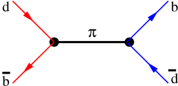
Figure 52: Top-pion contribution to $B^{0}-\bar{B}^{0}$ mixing.

In the top-pion graph of Fig.(52) we find a dangerously large contribution to $\delta m^{2}/m^{2}$, about two orders of magnitude above the experimental limit if normal CKM angles are assumed in a $(D:11)$ solution. However, owing to chirality the graph is proportional to the product $D_{L,3,1}D^{\dagger}_{R,3,1}$. Hence, we can systematically suppress this effect if we allow one of the three solutions $(D:10)$, or $(D:01)$, or $(D:00)$, while $(D:11)$ is disallowed. However, the topgluon graph yields a result that is similarly large, and proportional to $|D^{3,1}_{L}|^{2}+|D^{3,1}_{R}|^{2}$ [409]. Hence, we conclude that only the symmetric solution, $(D:00)$, is allowed, i.e., the off-diagonal mass matrix elements mixing $(1,3)$ in the down quark sector are all small. This suppresses Topcolor $b\rightarrow s\gamma$ effects as well.

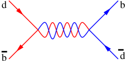
Figure 53: Top-gluon contribution to $B^{0}-\bar{B}^{0}$ mixing.

Thus, the CKM matrix elements mixing to the third generation must be controlled by $U_{L}$, and we thus require a $(U:10)$ or $(U:11)$ solution. The same effects occur in $D^{0}-\bar{D}^{0}$ mixing, where top-pion graphs are $\propto U_{L}U^{\dagger}_{R}$ off-diagonal elements, and topgluon graphs yield an expression $\propto|U_{L}|^{2}+|U_{R}|^{2}$. Therefore, the latter result implies that $D^{0}-\bar{D}^{0}$ must be in excess of the Standard Model prediction by about two orders of magnitude. This is close to the current experimental limit. Thus, $D^{0}-\bar{D}^{0}$ mixing emerges as an intriguing probe of topcolor. Data showing that the rate of $D^{0}-\bar{D}^{0}$ mixing is close to the SM prediction would pose a severe difficulty for topcolor models.

There are various other effects and limits on the models that can be obtained in mostly B and D, and to a lesser degree in K physics. Many of these are sensitive to the $Z^{\prime}$ which is more model dependent. We refer the interested reader to some of the relevant literature, beginning with [407], [427] and [428].

The measurement of $R_{b}$ in $Z\rightarrow b\bar{b}$ also yields an important constraint, [429], [239], [430]. This is subject to larger uncertainties because subleading $1/N_{c}$ top-pion loops dominate the leading large $N_{c}$ top-gluon loops. The degree of uncertainty can be seen by examining the analysis of [239] and noting that in their exclusion figure, with the Topcolor $f_{\pi}\sim 60$ GeV the model appears to be ruled out for all reasonable top-pion masses, while for $f_{\pi}\sim 100$ GeV there is no constraint. We take the difference of these two results to be within the errors of the subleading $N_{c}$ calculation. Similar uncertainties plague efforts to evaluate the oblique electroweak constraints on these models [430]. Also, diagrams that generate off-shell longitudinal mixing of the $Z$ with $\pi^{0}$ have not been included in any of these analyses.

Studying questions related to flavor physics in the context of Topcolor models has proven to be quite instructive. We now turn to other phenomenological questions and evaluate the status of limits on Topcolor scenarios.

4.3 Topcolor Phenomenology

4.3.1 Top-pions

If Topcolor produces a $\bar{t}t$ condensate to elevate the top quark mass, it necessarily produces an isovector of PNGB top-pions $\sim$ $t\bar{b},t\bar{t}-b\bar{b}$ and $b\bar{t}$. There may also be a heavier top-Higgs $\sim t\bar{t}+b\bar{b}$. In TC2 this multiplet of top-pions is uneaten by gauge bosons and the masses of these objects have been estimated in minimal schemes to be of order $\sim 200$ GeV, though this is fairly uncertain. The top-pions are strongly coupled to $\bar{t}t$, $\bar{b}b$ and $\bar{t}b$.

Top-pion vertex corrections therefore can noticeably decrease $R_{b}$ [239, 430], though the estimates are very sensitive to choice of $f_{\pi}$ (the effect becomes negligible with $f_{\pi}\sim 100$ GeV). Additional physics can in principle cancel the effect [238] (e.g., topgluons, for example, can increase $R_{b}$ [429]), but ref. [239] surveyed a number of possible sources of cancellation and found none producing an effect of the requisite size. Exchange of the light composite pseudoscalars in top seesaw models likewise contributes to the $T$ parameter. The interplay of the resulting limits is discussed in section 4.5. Several searches for top–pion and top–higgs ($\sigma$) production have been proposed; we now review these.

(i) Neutral Top–pions, Top–Higgs

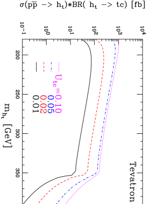
Figure 54: Top-higgs production cross-section via gluon fusion times branching ratio to $\bar{t}c$ at $\sqrt{s}=$ 2 TeV. [431]

A singly-produced neutral $\hat{\pi}^{0}$ that dominantly decays to $\bar{t}c$, via flavor mixing, could possibly be detected [431] at Run IIb or the LHC. The strength of the $\hat{\pi}^{0}$ coupling to $\bar{t}c$ is governed by the model-dependent parameter $U_{tc}\equiv\sqrt{|U^{L}_{tc}|^{2}+|U^{R}_{tc}|^{2}}$ where $U^{L}$ and $U^{R}$ are the matrices that diagonalize the up-quark mass matrix. In order for the flavor-changing decay to dominate, the decays to $t\bar{t}$ must be energetically disallowed. Decays to the electroweak gauge bosons is more model-dependent. In TC2 models, where the Yukawa coupling of scalars coupling to $t_{R}$ is enhanced by $r^{2}\approx(m_{t}/f_{\pi_{t}})^{2}\approx 10$, the top-scalar coupling to vector boson pairs is likewise suppressed by $1/r^{2}$ [432]. In top seesaw models (Section 4.4), $r=1$ so that the CP-even scalar decays mainly to $VV$; however, there can also be a light CP-odd scalar that is unable to decay to $VV$ and therefore decays to $\bar{t}c$ instead [246].

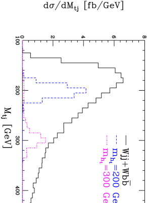
Figure 55: Mass distribution for the $\bar{t}c$ jet system for $m_{h_{t}}=200,300$ GeV and for the $Wjj$ and $Wbb$ backgrounds at $\sqrt{s}=$ $2$ TeV [431].

As shown in Figure 54, the production cross-section times flavor-changing branching ratio at Run IIb can provide several hundred top-higgs events even for $U_{tc}\sim 0.02$. Since the top-higgs is expected to be rather narrow, the signal peak should be visible for scalar masses up to the top threshold (see figure 55). At LHC, the production rate is dramatically enhanced since the primary production mode is gluon-gluon fusion; the cross-section times branching ratio is about 100 times that shown in Figure 54 for the same values of $U_{tc}$. Recent studies are optimistic for this process [433], but detailed background studies are required.

Recent work [434, 435, 436, 437] also suggests that $\hat{\pi}^{0}$’s may be visible through their $\bar{t}c$ decays at a LC running in $e^{+}e^{-}$ or $\gamma\gamma$ collision mode. The cross-section for $e^{+}e^{-}\to\bar{t}c$ or $\gamma\gamma\to\bar{t}c$ at a linear collider receives a contribution of order $20$ fb from neutral top-pions; an integrated luminosity of $50$ fb^-1 might make the top-pion visible [435]. On the other hand, the processes $e^{+}e^{-}\to\gamma\pi_{t},Z\pi_{t}$, with $\pi_{t}\to\bar{t}c$, have cross-sections of order $1.5$ pb and $0.3$ pb, respectively for top-pion masses below $350$ GeV [434]. A LC with $\sqrt{s}=1$ TeV would produce of order $400$ $(100)$ $\gamma\bar{t}c$ ($Z\bar{t}c$) events due to top-pions, potentially making both channels observable.

(ii) Charged Top–pions

In the presence of sizeable flavor-changing couplings $\bar{t}c$ of the $\hat{\pi}_{t}^{0}$, a large flavor-mixing coupling for the charged top-pions $\bar{c}b\pi_{t}^{+}$ can be induced [438]. This enables charged top-pions to be singly produced at sizeable rates in the s-channel at hadron colliders [439] or photon-photon linear colliders [440]. Ref.[438] has calculated the production cross-sections for several charged top-pion masses at a variety of colliders using the following benchmark set of couplings (typical for topcolor models): $U^{L}_{tb}=U^{L}_{cb}=0$, $U^{R}_{tb}=5U^{R}_{cb}$, $g_{\pi tb}=3\sqrt{2}m_{t}/v$. As shown in Figure 56, the cross-sections for Run II and the LHC are 4.0 pb and 0.55pb, respectively; those at photon-photon colliders are also sizeable. Hence, the authors of [438] suggest that charged top-pions would be visible up to masses of 300-350 GeV at Run II and  1 TeV at LHC, and that light enough top-pions would also be detectable at a linear collider running in the photon-photon mode.

In contrast, the work of ref [216] suggests that it will be difficult to detect the effects of charged top-pions on single top production at an $e\gamma$ collider in the process $e\gamma\to\bar{t}b\nu$.

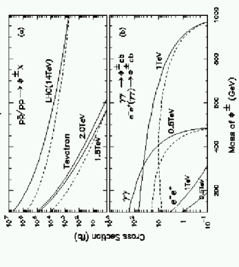
Figure 56: $s$-channel charged top-pion production with the benchmark Yukawa couplings given in the text. For reference, the dashed curves show the results for Yukawa couplings satisfying the 3-sigma $R_{b}$ bound [438].

We mention that in titling scenarios and variant schemes, there will be analogous bottom-pions which couple strongly to $\bar{b}b$. For a discussion of the associated phenomenology of these objects see [441, 442, 417].

4.3.2 Colorons: New Colored Gauge Bosons

Several of the dynamical models we have discussed include extended strong interactions $SU(3)_{1}\times SU(3)_{2}$, with coupling constants $h_{2}\gg h_{1}$. A general prediction of such models is the existence of a color-octet of massive gauge bosons (colorons). The best search strategy for colorons depends on how they couple to the different quark flavors. We will discuss the phenomenology resulting from the two most common choices for the quarks’ charge assignments.

(i) Topgluons

In models such as Topcolor [304], TC2 [274, 407], or Top Seesaw [245], only the third-generation quarks transform principally under the stronger $SU(3)_{2}$ group. As a result, the massive topgluons ($B^{\mu a}$) couple predominantly to third-generation quarks [304]. The topgluons are expected to be heavy ($M~{}0.5-2.0$ TeV) and broad ($\Gamma/M~{}0.3-0.7$) resonances. In production at, e.g., the Tevatron, in the dominant process $\bar{q}q\rightarrow(g,B)\rightarrow\bar{t}t$ the amplitude involves $(g_{3}\tan\theta)\times(-g_{3}\cot\theta)$ so that the factors involving $\theta$ cancel (and there is characteristic destructive interference above threshold). Thus, $\theta$ affects the rates only through the decay width of $B^{\mu a}$.

Topgluons of moderate mass may be produced directly at the Tevatron [187, 443]. CDF has recently used their measured upper limit on cross-section time branching ratio of new resonances decaying to $b\bar{b}$ to place a limit on topgluons [346] . They exclude topgluons of width $\Gamma_{B}=0.3M$ in the mass range $280<M<670$ GeV, of width 0.5 M in the range $340<M<640$ GeV, and of width $\Gamma_{B}=0.7M$ in the range $375<M<560$ GeV. A simulation of topgluon production and decay combined with an extrapolation of the CDF $b$-tagged dijet mass data from Run I [444] indicates that in Run IIb, the topgluon discovery mass reach in $b\bar{b}$ final states should be 0.77-0.95 TeV with 2 $fb^{-1}$ of integrated luminosity and 1.0 - 1.2 TeV with 30fb^-1.

Figure 57: CDF search for topgluons in $\bf b\bar{b}$ [346]

Figure 58: Invariant mass distribution for top pairs: pairs: D0 data (histogram), simulated background (triangles), simulated S+B (dots). In (a) $m_{t}$ unconstrained; in (b) $m_{t}=173$ GeV.[445, 446, 447, 448]

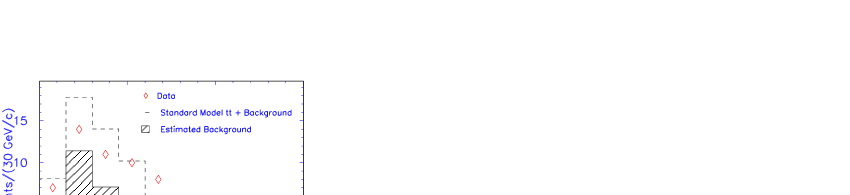
Figure 59: $P_{T}$ distribution for hadronically-decaying tops in lepton+jets events from CDF.[449]

Lower backgrounds make topgluons easier to find in their decays to top quarks [187, 443]. Initial measurements of the invariant mass ($M_{tt}$) and transverse momentum ($p_{T}$) distributions of the produced top quarks have been made, as shown in Figure 58. While a comparison with the measured $M_{jj}$ distribution for QCD dijets [450] illustrates how statistics-limited the Run I top sample is, some preliminary limits on new physics are being extracted. The $p_{T}$ distribution for the hadronically-decaying top in fully-reconstructed lepton + jets events (Figure 59) constrains any non-SM physics which increases the number of high-$p_{T}$ events. The fraction $R_{4}=0.000^{+0.031}_{-0.000}(stat)^{+0.024}_{-0.000}(sys)$ of events in the highest $p_{T}$ bin ($225\leq p_{T}\leq 300$ GeV) implies [449] a 95% c.l. upper bound $R_{4}\leq 0.16$ as compared with the SM prediction $R_{4}$ = 0.025.

In Run IIb, the $\sigma_{tt}$ measurement will be dominated by systematic uncertainties; the collaborations will use the large data sample to reduce reliance on simulations [452]. Acceptance issues such as initial state radiation, the jet energy scale, and the $b$-tagging efficiency will be studied directly in the data. It is anticipated [452] that an integrated luminosity of $1$ $(10,100)$ fb^-1 will enable $\sigma_{tt}$ to be measured to $\pm$ $11$ $(6,5)$ %. Topgluons of mass up to $1.0$-$1.1$ TeV ($1.3-1.4$ TeV) would be visible in 2 fb^-1 (30 fb^-1) at Run IIb, either in a search for a new broad resonance, or through their effects on the magnitude of the $t\bar{t}$ total cross-section. Projected Run IIb limits on $\sigma\cdot B$ for new resonances decaying to $t\bar{t}$ are illustrated in Figure 64. For further details on current and future topgluon searches at the Tevatron, see Table III of ref. [194]. The situation at the LHC and VLHC has been recently studied in considerable in [443], conclude that $\bar{t}t$ is overwhelmed by QCD backgrounds.

(ii) Flavor-universal Colorons

In theories in which all quarks carry only $SU(3)_{2}$ charge [420, 331, 421], the massive colorons couple with equal strength to all quark flavors (section 4.1.2(ii)). As a result, they will appear in dijet production and heavy flavor production at hadron colliders. A comparison of these processes [453] has indicated that the limits on colorons from dijet production should be the more stringent ones.

Existing limits on flavor-universal colorons from several sources are summaried in Figure 60. Exchange of light strongly-coupled colorons across quark loops would cause large contributions to the $T$ parameter; accordingly, the region $(M/\cot\theta)<450$ GeV is excluded. Light narrow colorons would have been seen by a Run I CDF search for new particles decaying to dijets (see [455]); this excludes the cross-hatched region at low $\cot^{2}\theta$. The light-shaded region $(M/\cot\theta<759$ GeV) is excluded by the shape of the dijet angular distribution measured by D0 [456]. Finally, the shape of the dijet mass spectrum measured by D0 [450] sets the strongest limit: $M/\cot\theta>837$ GeV [455].

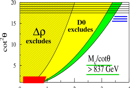
Figure 60: Experimental limits on flavor-universal colorons from sources described in the text [455]. The horizontally hatched region at large $\cot\theta$ is not part of the Higgs phase of the model [420].

In the context of flavor-universal TC2 models, the value of $\kappa_{3}$ must be approximately $2$ in order for the colorons to help cause the top quark to condense as discussed earlier [421]; this is equivalent to $\cot\theta\approx 4$. Hence, in these models, the limit set by D0 on the coloron mass is $M_{c}>3.4$ TeV.

Run IIb will, naturally, be sensitive to somewhat heavier colorons. According to the TeV 2000 report the limit on $\sigma\cdot B$ will improve as shown in Figure 61. The predicted $\sigma\cdot B$ for a coloron of $\cot\theta=1$ is equivalent to that for an axigluon (shown); larger values of $\cot\theta$ increase the rate.

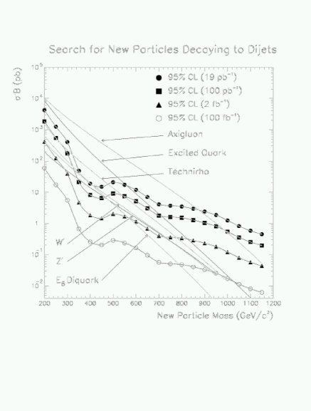
Figure 61: Anticipated 95% c.l. upper limit on $\sigma\cdot B$ for new particles decaying to dijet as a function of the new particle mass for various integrated luminosities at the Tevatron. Axigluon curve corresponds to a coloron of $\cot\theta=1$[452].

4.3.3 New $Z^{\prime}$ Bosons

As discussed in section 4.1, both Classic TC2 [274, 407] and Flavor-Universal TC2 [331, 421] models include an extra $U(1)$ group and predict the presence of a massive $Z^{\prime}$ boson. The couplings of this $Z^{\prime}$ to fermions are generally not flavor-universal, and the more strongly suppressed the $Z^{\prime}$ couplings to first and second generation fermions are, the less effective traditional searches for $Z^{\prime}$ become. This section discusses experimental searches and limits that exploit the flavor non-universal couplings of the $Z^{\prime}$.

TC2 models include an extended electroweak sector of the form

$$SU(2)_{W}\times U(1)_{h}\times U(1)_{\ell}\ .$$ (4.168)

where the coupling of the first $U(1)$ group is the stronger one, $g_{h}>>g_{\ell}$. At a scale above the weak scale, the two hypercharge groups break to a subgroup identified as $U(1)_{Y}$. As a result, a $Z^{\prime}$ boson that is a linear combination of the original two hypercharge bosons becomes massive. This heavy $Z^{\prime}$ boson couples to a fermion as

$$-i\frac{e}{\cos\theta}\left(\frac{s_{\chi}}{c_{\chi}}Y_{\ell}-\frac{c_{\chi}}{s_{\chi}}Y_{h}\right)$$ (4.169)

where $Y_{h}$ ($Y_{\ell}$) is the fermion’s hypercharge under the $U(1)_{h}$ ($U(1)_{\ell}$) group and $\chi$ is the mixing angle between the two original hypercharge sectors $\cot{\chi}=(g_{h}/g_{\ell})^{2}$. Compared with the couplings of the $Z^{\prime}$ boson from an extended weak group (Section 3.6.5), the significant physical differences are that the overall coupling is of hypercharge rather than weak strength, and the $Z^{\prime}$ couples to both left-handed and right-handed fermions at leading order.

Figure 62: Lower bounds at 95% c.l. on mass of “optimal” non-universal Z’ boson. [278]. Solid curve is from a global fit to precision electroweak data; dashed line is from LEP II contact interaction limits. The bottom plot is a close-up of the region where the smallest Z’ mass is allowed.

(i) $Z^{\prime}$ and Precision Tests

Studies of precision electroweak limits on the $Z^{\prime}$ bosons [278, 457] in these models have obtained lower bounds on $M_{Z^{\prime}}$ as a function of $\sin^{2}\chi$. The lower bound is found to depend quite strongly on the hypercharge assignments of the fermions because the shift in the Z boson’s coupling to fermions depends directly on $Y_{h}$:

$$\delta g^{f}\approx-\left(\frac{e\sin\theta}{x\cos\theta\cos^{2}\chi}\right)\left(1+\frac{\epsilon}{\sin^{2}\chi}\right)\left[Y_{h}^{f}-\sin^{2}\chi Y^{f}\right]$$ (4.170)

where $\epsilon\equiv 2f_{\pi_{t}}^{2}/v^{2}(Y_{h}^{t_{L}}-Y_{h}^{t_{R}})$. In models with a so-called “optimal” $Z^{\prime}$, in which the third generation fermions have $Y_{h}=Y,\,Y_{\ell}=0$ and those of the other two generations have $Y_{h}=0,\,Y_{\ell}=Y$, the $Z^{\prime}$ can be as light as $630$ GeV (see figure 62) at 95% c.l. for $\sin^{2}\chi\approx 0.0784$; a $Z^{\prime}$ mass less than a TeV is allowed for $0.0744\begin{array}[]{c}\,\sim\vspace{-21pt}\\ <\end{array}\sin^{2}\chi\begin{array}[]{c}\,\sim\vspace{-21pt}\\ <\end{array}0.0844$ [278]. In the TC2 model of Lane [330], where the fermions have considerably larger $Y_{h}$ charges (see table), the lower bound on the $Z^{\prime}$ mass is correspondingly higher, about $20$ TeV. The strong constraint here comes from sensitivity to atomic parity violation in $Cs$ [330]. A variant of Lane’s model [458] in which the lepton’s $U(1)_{h}$ couplings are vectorial has a $Z^{\prime}$ limit much closer to that of the “optimal” scenario (though lacking the low-mass region near $\sin^{2}\chi=.0784$) [457].

1st, 2nd	$Y_{h}$	3rd	$Y_{h}$
$(u,d)_{L},\ (c,s)_{L}$	-10.5833	$(t,b)_{L}$	8.7666
$u_{R},\ c_{R}$	-5.78333	$t_{R}$	11.4166
$d_{R},\ s_{R}$	-6.78333	$b_{R}$	10.4166
$(\nu_{e},e)_{L},\ (\nu_{\mu},\mu)_{L}$	-1.54	$(\nu_{\tau},\tau)_{L}$	-1.54
$e_{R},\ \mu_{R}$	2.26	$\tau_{R}$	2.26

Table 6: Fermion charges for Lane’s model [330]

The non-universal couplings of the $Z^{\prime}$ boson to fermions cause it to induce lepton number violating processes. A study in ref. [459] has shown that $\mu-e$ conversion in nuclei is about an order of magnitude better than the decay $\mu\to 3e$ [460] for constraining the magnitudes of the lepton mixing angles. The decay $\mu\to e\gamma$ yields weaker bounds. Present data allows the $Z^{\prime}$ mass to be as large as 1 TeV and the magnitudes of the lepton mixing angles lie roughly between the analogous CKM entries and their square-roots [459]. Looking to the future, ref. [461] finds that the MECO and PRIME experiments will probe lepton flavor violating $Z^{\prime}$ bosons out to a mass of order $10$ TeV, far better than the MEG ($\mu\to e\gamma$) experiment can do.

At energies well below the mass of the $Z^{\prime}$ boson, its exchange in the process $e^{+}e^{-}\to f\bar{f}$ where $f$ is a $\tau$ lepton or $b$ quark may be approximated by four-fermion contact interactions. As discussed in section 3.6.5, limits the ALEPH and OPAL experiments have given on the scale $\Lambda$ of new contact interactions may be translated into lower bounds on the mass of the $Z^{\prime}$ boson. The strongest such limits on an “optimal” $Z^{\prime}$ boson are for the process $e^{+}_{R}e^{-}_{R}\to\tau^{+}_{R}\tau^{-}_{R}$ [329]

$$M_{Z^{\prime}}=\Lambda\sqrt{\alpha_{em}/\cos^{2}\theta}\ >\ \left\{\ {370\ {\rm GeV}\ \ \ {\rm ALEPH}}\atop{370\ {\rm GeV}\ \ \ {\rm OPAL}}\right\}\ .$$ (4.171)

which improves a bit on the limit from precision electroweak data [457].

Figure 63: The 95% c.l. upper limits on $\sigma_{X}\cdot BR{X\to t\bar{t}}$ as a function of mass (solid and open points) compared to the cross section for a leptophobic topcolor $Z^{\prime}$ (thick solid and dashed curves) for two resonance widths [451].

Figure 64: Anticipated[452] Run IIb limits on $\sigma\cdot B(X\to t\bar{t})$ and predictions for a topcolor Z’.

Dijet and Drell-Yan data from CDF and D0 can, likewise, be interpreted as setting limits on the mass of a new $Z^{\prime}$ boson. The lower bounds on an “optimal” $Z^{\prime}$ derived from limits on quark-lepton contact interactions are significantly weaker than those from the LEP data [329]. The constraints on the $Z^{\prime}$ of Lane’s TC2 model [330] from dijet and Drell-Yan data are sufficient to indicate that the model requires significant fine-tuning [462]; as mentioned earlier, however, the bounds from precision electroweak data are even stronger.

(ii) $Z^{\prime}$ Production Searches

Evidence of a $Z^{\prime}$ boson coupled primarily to the third generation can more profitably be sought in heavy flavor production at the Tevatron. The CDF collaboration has searched in $t\bar{t}$ events [451] for a narrow leptophobic $Z^{\prime}$ boson present in some models of topcolor-assisted technicolor [463]. Finding no evidence of a new narrow residence, CDF sets the limits $M_{Z^{\prime}}>780$ GeV for such a $Z^{\prime}$ of natural width $\Gamma_{Z^{\prime}}=0.04M_{Z^{\prime}}$ and $M_{Z^{\prime}}>480$ GeV for $\Gamma_{Z^{\prime}}=0.012M_{Z^{\prime}}$ as shown in figure 63. Simulations of $Z^{\prime}\to t\bar{t}\to l\nu b\bar{b}jj$ for Run II indicate that with 2$fb^{-1}$ (30 fb${-1}$) of data a narrow topcolor $Z^{\prime}$ of mass up to 0.92 TeV (1.15 TeV) would be visible [452]; figure 64 summarizes the anticipated Run II sensitivity to $\sigma\cdot B$ in the $M_{tt}$ distribution, and the corresponding predictions for topcolor $Z^{\prime}$ bosons.. The search by the CDF Collaboration for new resonances decaying to $b\bar{b}$ [346], which was previously mentioned (section 4.3.2, figure 57) as setting limits on technirhos, falls slightly short of setting a limit on topcolor $Z^{\prime}$ bosons. In addition to pursuing Z’ bosons in these heavy quark channels, the Run IIb will also be able to look for $Z^{\prime}$ bosons decaying to $\tau$ leptons as described in section 3.6.5. In the case with the lowest standard model background, $Z^{\prime}\to\tau\tau\to e\mu\nu\bar{\nu}$, a $Z^{\prime}$ boson with a mass up to about 600 GeV should be accessible (depending on mixing angle) [329]. For further details on current and future Topcolor $Z^{\prime}$ boson searches at the Tevatron, see Table IV of ref. [194].

A $Z^{\prime}$ boson would also be visible in the process $e^{+}e^{-}\to\tau\tau$ at an NLC [421]. Assuming a $50$% efficiency for idenitfying $\tau$–pairs and requiring an excess over standard model backgrounds of $(N^{\tau\tau}-N^{\tau\tau}_{SM})\geq 5\sqrt{N^{\tau\tau}_{SM}}$, it appears that the effects of a 2.7 TeV $Z^{\prime}$ boson with $\alpha_{1}\tan^{2}\chi\leq 1$ would be visible in a 50 fb^-1 sample taken at $\sqrt{s}=500$ GeV. A $1.5$ TeV NLC with 200 fb^-1 of data would be sensitive to $Z^{\prime}$ bosons as heavy as 6.6 TeV. The other channels suggested earlier in the context of topflavor models might also be useful for finding this $Z^{\prime}$ at a LC, LHC, or FMC.

4.4 Top Seesaw

The electroweak mass gap, i.e., the dynamical fermion mass associated with the generation of $v_{weak}$ through the Pagels-Stokar relation eq.(4.138), is $\sim 600$ GeV when the scale of Topcolor is taken to be a natural scale of order $\sim 1$ TeV. If the top quark mass were this large, our problems would be solved, and EWSB would be identified naturally with a $\bar{t}t$ condensate. By itself, however, the top quark is too light to produce the full electroweak condensate in this way.

We can, however, write a viable model in which the $I=\frac{1}{2}$ top quark mass term, the term associated with electroweak symmetry breaking, is indeed $\sim 600$ GeV, and exploit a seesaw mechanism to tune the physical mass of the top quark to $m_{t}=175$ GeV [245, 246]. This gives up the predictivity of the top quark mass, since the tuning is done through a new mixing angle. Because the top quark is heavy, however, the mixing angle need not be chosen artificially small.

The Top Seesaw mechanism can be implemented with the introduction of a pair of iso-singlet, vectorlike quarks, $\chi_{L}$ and $\chi_{R}$ which both have $Y=4/3$, analogues of the $t_{R}$. This model produces a bound-state Higgs boson, primarily composed of $\bar{t}_{L}\chi_{R}$, with the Higgs mass $\sim 1$ TeV, saturating the unitarity bound of the Standard Model. Such a large Higgs mass would seemingly be a priori ruled out by the $S-T$ parameter constraints. Remarkably, however, the Top Seesaw theory has the added bonus of supplying a rather large $T$-parameter contribution associated with the presence of the $\chi$ fermions [245, 464].

In 1998 when the Top Seesaw theory was proposed, it was in poor agreement with the $S-T$ bounds. With the most recent compilation of LEP and worldwide data, including a refined initial state radiation and $W$-mass determination, the Top Seesaw theory lies within the $95\%$ c.l. error ellipse (see Section 4.5). Indeed the theory lies within the $S-T$ plot for expected natural values of the $\chi$ masses. Hence, the theory has already scored a predictive success: the $S-T$ ellipse has moved to accomodate it. We may, in fact, view the measured error ellipse as a determination of the $\chi$ mass in this scheme; we obtain roughly $M_{\chi}\sim 4$ TeV. In this picture, the worldwide electroweak precision measurements are probing the mass of a heavy new particle, the $\chi$, significantly above the electroweak scale.

Note that the Top Seesaw model, unlike TC2, does not invoke Technicolor; rather, it replaces Technicolor entirely with Topcolor. It offers novel model building possibilities for attacking the flavor problem [465, 466, 417, 467]. Extensions have been constructed in which the $W$, $Z$, $t$ and $b$ all receive dynamical masses. Construction of an explicit model of all quark and lepton masses seems plausible [465, 466]. Because the $\chi$ quarks need not carry weak-isospin quantum numbers, and enter in vectorlike pairs, the constraints on the number of techniquarks from the $S$ parameter are essentially irrelevant for the Top Seesaw. The Top Seesaw also finds an attractive setting in extra dimensional models, as discussed in Section 4.6. The $\chi$ quarks and Topcolor itself may be interpreted as Kaluza-Klein modes. Because the mass-gap is $600$ GeV rather than $m_{t}=175$ GeV, the masses of all the colorons, and any additional heavy gauge bosons, are naturally moved to slightly larger mass scales than in TC2. One then has more model-building elbow room: phenomenological exploration of the Top Seesaw dynamics will rely on the VLHC rather than the LHC.

4.4.1 The Minimal Model

In the minimal Top Seesaw scheme the full EWSB occurs via the condensation of the left-handed top quark with a new, right-handed weak-singlet quark, which we refer to as a $\chi$-quark. The $\chi_{R}$ quark has hypercharge $Y=4/3$ and is thus indistinguishable from the $t_{R}$. The dynamics which leads to this condensate is Topcolor, as discussed below, and no tilting $U(1)^{\prime}$ is required. The fermionic mass scale of this weak-isospin $I=1/2$ condensate is $\sim 0.6$ TeV. This corresponds to the formation of a dynamical bound-state weak-doublet Higgs field, $H\sim(\overline{\chi_{R}}t_{L},\overline{\chi_{R}}b_{L})$. To leading order in $1/N_{c}$ this yields a VEV for the Higgs boson, via the Pagels-Stokar formula, of the appropriate electroweak scale, $v_{weak}=175$ GeV, and the top quark acquires an $I=\frac{1}{2}$ dynamical mass $\mu$. The ($I=0$, $Y=4/3$) $\chi$-quarks have an allowed Dirac mass $M_{\chi}$ and a mass term $m_{0}$ that mixes $t_{R}$ and $\chi_{L}$. Thus, the full fermionic mass matrix takes the form:

$$\overline{\left(\begin{array}[]{c}t_{L}\\ \chi_{L}\end{array}\right)}\left(\begin{array}[]{cc}0&\mu\\ m_{0}&M_{\chi}\end{array}\right)\left(\begin{array}[]{c}t_{R}\\ \chi_{R}\end{array}\right)$$ (4.172)

where the vanishing entry is a term forbidden by the Topcolor assignments (see 4.4.2 below). We diagonalize the mass matrix:

$${\cal M}=U_{L}^{\dagger}(\phi_{L}){\cal M}_{D}U_{R}(\phi_{R})$$ (4.173)

leading to eigenvalues:

$${\cal M}_{D}=\left(\begin{array}[]{cc}m_{1}&0\\ 0&m_{2}\end{array}\right)$$ (4.174)

where:

$$m_{1}^{2} = \frac{1}{2}\left[{m_{0}^{2}+M_{\chi}^{2}+\mu^{2}}-{\sqrt{\left(m_{0}^{2}+M_{\chi}^{2}+\mu^{2}\right)^{2}-4\mu^{2}m_{0}^{2}}}\right]\vskip 12.0pt plus 4.0pt minus 4.0pt$$ (4.175)

$$\approx \frac{m_{0}^{2}\mu^{2}}{M_{\chi}^{2}+m_{0}^{2}+\mu^{2}}+{\cal O}(m_{0}^{4}\mu^{4}/M_{\chi}^{6})$$

and

$$m_{2}^{2} = \frac{1}{2}\left[{m_{0}^{2}+M_{\chi}^{2}+\mu^{2}}+{\sqrt{\left(m_{0}^{2}+M_{\chi}^{2}+\mu^{2}\right)^{2}-4\mu^{2}m_{0}^{2}}}\right]\vskip 12.0pt plus 4.0pt minus 4.0pt$$ (4.176)

$$\approx M_{\chi}^{2}+m_{0}^{2}+\mu^{2}+{\cal O}(m_{0}^{2}\mu^{2}/M_{\chi}^{2})$$

where limits for large $M_{\chi}$ are indicated.

The fermionic mass matrix thus admits a conventional seesaw mechanism, yielding the physical top quark mass as an eigenvalue that is $\sim m_{0}\mu/M_{\chi}<<\mu\approx 600$ GeV. The top quark mass can be adjusted to its experimental value. The diagonalization of the fermionic mass matrix does not affect the VEV ($v_{weak}=175$ GeV) of the composite Higgs doublet. Indeed, the Pagels-Stokar formula is now modified to read:

$$v_{weak}^{2}\equiv f_{\pi}^{2}=\frac{N_{c}}{16\pi^{2}}\frac{m_{t}^{2}}{\sin^{2}\phi_{L}}(\log\frac{M^{2}}{\overline{M}^{2}}+k)$$ (4.177)

where $m_{t}$ is the physical top mass, and $\phi_{R}$ the mass matrix diagonalizing mixing angle. The Pagels-Stokar formula differs from that obtained (in large $N_{c}$ approximation) for top quark condensation models by the large enhancement factor $1/\sin^{2}\phi_{L}$. This is a direct consequence of the seesaw mechanism. The Top Seesaw employs $\psi_{L}=(t_{L},b_{L})$ as the source of the weak $I=1/2$ quantum number of the composite Higgs boson, and thus the origin of the EWSB vacuum condensate. This neatly separates [258] the problem of EWSB from that of the new weak-isosinglet states in the $\chi_{L,R}$ and $t_{R}$ sector, a distinct advantage since the electroweak constraints on new physics are not very restrictive of isosinglets.

4.4.2 Dynamical Issues

How does Topcolor produce the $\mu$ mass term? We introduce an embedding of QCD into the gauge groups $SU(3)_{1}\times SU(3)_{2}$, with coupling constants $h_{1}$ and $h_{2}$ respectively. These symmetry groups are broken down to $SU(3)_{QCD}$ at a high mass scale $M$. The assignment of the elementary fermions to representations under the full set of gauge groups $SU(3)_{1}\times SU(3)_{2}\times SU(2)_{W}\times U(1)_{Y}$ is as follows:

$$\psi_{L}:\,({\bf 3,1,2,}\,+1/3)\;\;\;,\;\;\ \chi_{R}:\,({\bf 3,1,1,}\,+4/3)\;\;\;,\;\;\ t_{R},\chi_{L}:\,({\bf 1,3,1,}\,+4/3)~{}.$$ (4.178)

This set of fermions is incomplete: the representation specified has $[SU(3)_{1}]^{3}$, $[SU(3)_{2}]^{3}$, and $U(1)_{Y}[SU(3)_{1,2}]^{2}$ gauge anomalies. These anomalies will be canceled by fermions associated with either the dynamical breaking of $SU(3)_{1}\times SU(3)_{2}$, or with the $b$-quark mass generation (a specific example of the latter case is given at the end of this section).

Schematically things look like this:

$\ \ \ \ \ \ \ \ \ \ SU(3)_{1}$        $\ \ \ \ SU(3)_{2}$

$\left(\begin{array}[]{c}\left(\begin{array}[]{c}t\\ b\end{array}\right)_{L}\\ \left(\chi\right)_{R}\\ ...\end{array}\right)$     $\left(\begin{array}[]{c}\left(\begin{array}[]{c}t\\ b\end{array}\right)_{R}\\ \left(\chi\right)_{L}\\ ...\end{array}\right)$

The dynamics of EWSB and top-quark mass generation will not depend on the details of the additional fermions.

We introduce a scalar Higgs field, $\Phi$, transforming as $({\bf\overline{3},3,1,}\,0)$, which develops a diagonal VEV, $\langle\Phi{}^{i}_{j}\rangle={\cal V}\delta_{j}^{i}$. This field is presumably yet another dynamical condensate, or it can be interpreted as a relic of compactification of an extra dimension. Topcolor is then broken to QCD,

$$SU(3)_{1}\times SU(3)_{2}\longrightarrow SU(3)_{QCD}$$ (4.179)

yielding massless gluons and an octet of degenerate colorons with mass $M$ given by

$$M^{2}=(h_{1}^{2}+h_{2}^{2})\,{\cal V}^{2}\,.$$ (4.180)

We can also exploit $\Phi$ to provide the requisite $M_{\chi}$ by introducing a Yukawa coupling of the fermions $\chi_{L,R}$ of the form: $-\xi\,\overline{\chi_{R}}\,\Phi\,\chi_{L}+{\rm h.c.}\longrightarrow-M_{\chi}\,\overline{\chi}\chi$. We emphasize that this is an electroweak singlet mass term. $\xi$ can be a perturbative coupling constant so ${\cal V}\gg\xi{\cal V}=M_{\chi}$. Finally, since both $t_{R}$ and $\chi_{L}$ carry identical Topcolor and $U(1)_{Y}$ quantum numbers we are free to include the explicit mass term, also an electroweak singlet, of the form $m_{0}\overline{\chi_{L}}\,t_{R}+{\rm h.c.}$.

The Lagrangian of the model at scales below the coloron mass is $SU(3)_{C}\times SU(2)_{W}\times U(1)$ invariant and becomes:

$${\cal{L}}_{0}={\cal{L}}_{\rm kinetic}-(M_{\chi}\,\overline{\chi_{L}}\,\chi_{R}+m_{0}\,\overline{\chi_{L}}\,t_{R}+{\rm h.c.})+{\cal{L}}_{\rm int}$$ (4.181)

${\cal{L}}_{\rm int}$ contains the residual Topcolor interactions from the exchange of the massive colorons:

$${\cal{L}}_{\rm int}=-\frac{h^{2}_{1}}{M^{2}}\left(\overline{\psi_{L}}\,\gamma^{\mu}\frac{M^{A}}{2}\psi_{L}\right)\left(\overline{\chi_{R}}\,\gamma_{\mu}\frac{M^{A}}{2}\chi_{R}\right)+LL+RR+...\;$$ (4.182)

where $LL$ $(RR)$ refers to purely left-handed (right-handed) current-current interactions. It suffices to retain in the low energy theory only the effects of the operators shown in eq. (4.182) even though higher dimension operators may be present. To leading order in $1/N_{c}$, upon performing the familiar Fierz rearrangement, we have:

$${\cal{L}}_{\rm int}=\frac{h_{1}^{2}}{M^{2}}(\overline{\psi_{L}}\,\chi_{R})\,(\overline{\chi_{R}}\,\psi_{L})~{}.$$ (4.183)

It is convenient to pass to a mass eigenbasis with the following redefinitions:

$$\chi_{R}\rightarrow\cos\phi_{R}\;\chi_{R}-\sin\phi_{R}\;t_{R}\,;\quad t_{R}\rightarrow\cos\phi_{R}\;t_{R}+\sin\phi_{R}\;\chi_{R}$$ (4.184)

where

$$\tan\phi_{R}=\frac{m_{0}}{M_{\chi}}$$ (4.185)

In this basis, the NJL Lagrangian takes the form:

$${\cal{L}}_{0} = {\cal{L}}_{\rm kinetic}-\overline{M}\,\overline{\chi_{R}}\,\chi_{L}+{\rm h.c.}$$ (4.186)

$$+\frac{h_{1}^{2}}{M^{2}}\left[\overline{\psi_{L}}\,\left(\cos\phi_{R}\;\chi_{R}-\sin\phi_{R}\;t_{R}\right)\right]\left[\left(\cos\phi_{R}\;\overline{\chi_{R}}-\sin\phi_{R}\;\overline{t_{R}}\right)\,\psi_{L}\right]$$

where

$$\overline{M}=\sqrt{M_{\chi}^{2}+m_{0}^{2}}~{}.$$ (4.187)

At this stage we have the choice of using the renormalization group, or looking at the mass gap equations for $\mu$. A rationale for studying the gap equations is that they in principle allow one to explore limits, such as $\overline{M}>M$ which are conceptually more difficult with the renormalization group. For a more complete analysis of the dynamics see [468].

Figure 65: Gap equations for $\mu_{1}$. A similar set of terms is obtained for $\mu_{2}$ [468].

Let us summarize the gap equation analysis. We assume two dynamical mass terms:

$$-\mu_{1}\overline{t}_{L}\chi_{R}-\mu_{2}\overline{t}_{L}t_{R}$$ (4.188)

and we compute the gap equations to order ${\cal{O}}(\mu^{3})$. This will produce no IR divergences in terms to order $\cos^{2}\phi_{R}$, but there is an IR log-divergence in the last term of Fig.(65) of order $\sin^{2}\phi_{R}$, and we take this to be $\ln(m_{t}^{2})$. Fig.(65) produces the coupled system of gap equations for $\mu_{1}$:

$$\mu_{1} = \frac{h_{1}^{2}N}{8\pi^{2}M^{2}}\mu_{1}\cos^{2}\phi_{R}\left(M^{2}-\overline{M}^{2}\ln\left(\frac{M^{2}+\overline{M}^{2}}{\overline{M}^{2}}\right)\right)$$ (4.189)

$$+\frac{h_{1}^{2}N}{8\pi^{2}M^{2}}\mu_{1}\cos^{2}\phi_{R}\left(-\mu_{1}^{2}\ln\left(\frac{M^{2}+\overline{M}^{2}}{\overline{M}^{2}}\right)+\frac{\mu_{1}^{2}M^{2}}{M^{2}+\overline{M}^{2}}-\mu_{2}^{2}\ln\left(\frac{M^{2}+\overline{M}^{2}}{\overline{M}^{2}}\right)\right)$$

$$+\frac{h_{1}^{2}N}{8\pi^{2}M^{2}}\mu_{2}\cos\phi_{R}\sin\phi_{R}\left(M^{2}-\mu_{1}^{2}\ln\left(\frac{M^{2}+\overline{M}^{2}}{\overline{M}^{2}}\right)-\mu_{2}^{2}\ln\left(\frac{M^{2}}{m_{t}^{2}}\right)\right)$$

and a similar set for $\mu_{2}$. With the substitutions $\mu_{1}=\mu\cos\phi_{R}$ and $\mu_{2}=\mu\sin\phi_{R}$ the two independent gap equations reduce to a single mass gap equation:

$$\mu = \frac{h_{1}^{2}N}{8\pi^{2}M^{2}}\mu\left(M^{2}-\overline{M}^{2}\cos^{2}\phi_{R}\ln\left(\frac{M^{2}+\overline{M}^{2}}{\overline{M}^{2}}\right)\right.$$ (4.190)

$$\left.-\mu^{2}\ln\left(\frac{M^{2}+\overline{M}^{2}}{\overline{M}^{2}}\right)+\frac{\mu^{2}M^{2}}{M^{2}+\overline{M}^{2}}-\mu^{2}\sin^{4}\phi_{R}\ln\left(\frac{M^{2}(M^{2}+\overline{M}^{2})}{m_{t}^{2}\overline{M}^{2}}\right)\right)$$

The gap equation eq.(4.190) shows that we require supercritical coupling as the mass $\overline{M}$ becomes large. Moreover, for fixed supercritical coupling, $h_{1}^{2}/4\pi$, as we raise the scale $\overline{M}$ the condensate turns off like a second order phase transition.

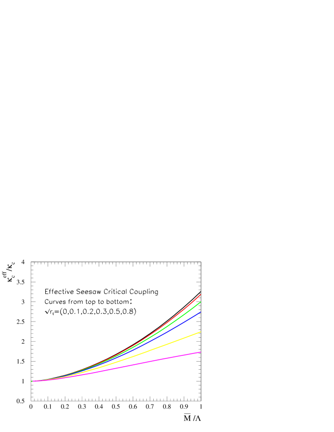
Figure 66: Gap equation with coupling constant $\kappa=h_{1}^{2}/4\pi$ (scaled by constant $\kappa_{c}\equiv 2\pi/3$) as a function of $\overline{M}/M$, for $\sqrt{\tan\phi_{R}}=(0,\,0.1,\,0.2,\,0.3,\,0.5,\,0.8)$. from Hill, He, and Tait [468]

We can also see that these reproduce normal top condensation in the decoupling limit. For example, choose $\overline{M}\rightarrow\infty$ for fixed $M$, and we find:

$$\mu = \frac{h_{1}^{2}N}{8\pi^{2}M^{2}}\mu\left(M^{2}(1-\cos^{2}\phi_{R})-\mu^{2}\sin^{2}\phi_{R}\ln\left(\frac{M^{2}}{m_{t}^{2}}\right)\right)$$ (4.191)

and redefining $\tilde{g}=h_{1}\sin\phi_{R}$, and $m_{t}=\mu\sin\phi_{R}$ we have:

$$m_{t} = \frac{\tilde{g}^{2}N}{8\pi^{2}M^{2}}\mu\left(M^{2}-m_{t}^{2}\ln\left(\frac{M^{2}}{m_{t}^{2}}\right)\right)$$ (4.192)

which is the top condensation gap equation. Here we have decoupled $\chi_{L}$ and $\chi_{R}$ with $\overline{M}\rightarrow\infty$. We can also obtain top condensation by setting $\sin^{2}\phi_{R}=0$ and $\overline{M}\rightarrow 0$, which decouples $\chi_{L}$ and $t_{R}$, and causes $\chi_{R}$ to play the role of $t_{R}$.

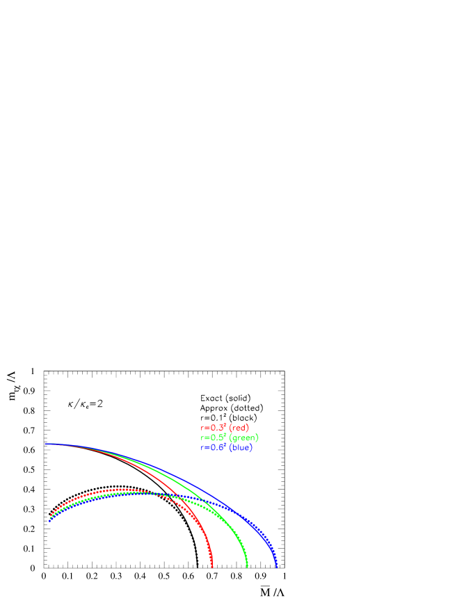
Figure 67: Behavior of gap equation for fixed supercritical coupling $h_{1}^{2}/4\pi\kappa_{c}=2.0$ as $\overline{M}/M$ is increased. In the notation of the figure, $m_{t\chi}=\mu$. $\sqrt{\tan\phi_{R}}=(0,\,0.1,\,0.2,\,0.3,\,0.5,\,0.8)$. The figure shows results for our gap equation (solid) and an approximation (dotted) that treats $\overline{M}$ as a mass insertion (see [468]).

A separate question of interest is the structure of the electroweak corrections in the Top Seesaw theory. This is most easily determined from an effective Lagrangian for the composite Higgs boson. The most complete study to date is that of Hill, He and Tait [468]. The composite Higgs boson mass satisfies the approximate NJL result, $m_{Higgs}\approx 2\mu\sim 1.2$ TeV. Experience with Topcolor suggests that radiative corrections from $SU(2)_{2}$ will reduce this. The composite Higgs mass is consistent with the unitarity limit of the Standard Model. By itself, this pulls the theory to large negative $T$. However, there are $\chi-t$ mixing corrections to the T parameter as well. We obtain for T:

$$T=\frac{Nm_{t}^{2}}{32\pi^{2}v_{weak}^{2}\alpha_{Z}}\left[\frac{\mu^{2}}{m_{0}^{2}}+\frac{2\mu^{2}}{\overline{M}^{2}}\left(\ln\left(\frac{\overline{M}^{4}}{\mu^{2}m_{0}^{2}}\right)-1\right)\right]$$ (4.193)

Putting in typical numbers, such as $\mu=0.6$ TeV, $m_{0}=m_{t}\overline{M}/\mu\approx 1.2$ TeV, $\alpha_{Z}=1/128$, one observes a large positive correction to $T$, and one recovers consistency with the error ellipse constraint for $\overline{M}\approx 4$ TeV. Note that the $S$-parameter is vanishing, since the additional $\chi$ quarks are weak isosinglets.

We note that, using the freedom to adjust $\sin\phi_{R}$, we can in principle dynamically accommodate any fermion mass lighter than $\sim 600$ GeV – at the price of some fine-tuning. This freedom may be useful in constructing more complete models involving all three generations [466, 465]. The top quark is unique, however, in that it is very difficult to accommodate such a heavy quark in any other way, and there is less apparent fine-tuning. We therefore believe it is generic, in any model of this kind, that the top quark receives the bulk of its mass through this seesaw mechanism. In a more general theory that includes the seesaw mechanism there are more composite scalars, and one of the neutral Higgs bosons may be as light as ${\cal O}(100$ GeV).

4.4.3 Including the $b$-quark

Inclusion of the $b$-quark is straightforward, and two distinct schemes immediately suggest themselves. We include additional fermionic fields of the form $\omega_{L}$, $\omega_{R}$, and $b_{R}$ with the assignments:

$$b_{R},\omega_{L}:\,({\bf 1,3,1,}-2/3)\;\;\;,\;\;\;\omega_{R}:\,({\bf 3,1,1,}-2/3)~{}.$$ (4.194)

These fermion gauge assignments cancel the anomalies noted above. We further allow $\overline{\omega_{L}}\omega_{R}$ and $\overline{\omega_{L}}b_{R}$ mass terms, in direct analogy to the $\chi$ and $t$ mass terms:

$${\cal{L}}_{0}\supset-(M_{\omega}\overline{\omega_{L}}\omega_{R}+m_{\omega}\overline{\omega_{L}}b_{R}+{\rm h.c.})$$ (4.195)

With the previous assignments for the $\chi$ quarks, schematically, this looks like the following:

Inclusion of b-quark I:

$\ \ \ \ \ \ \ \ \ \ \ \ SU(3)_{1}$                    $\ \ \ \ \ \ \ \ SU(3)_{2}$

$\left(\begin{array}[]{c}\left(\begin{array}[]{c}t\\ b\end{array}\right)_{L}I={\frac{1}{2}}\\ \left(\begin{array}[]{c}\chi\\ \omega\end{array}\right)_{R}I=0\end{array}\right)$     $\left(\begin{array}[]{c}\left(\begin{array}[]{c}t\\ b\end{array}\right)_{R}I=0\\ \left(\begin{array}[]{c}\chi\\ \omega\end{array}\right)_{L}I=0\end{array}\right)$

Alternatively, we may define the $\chi$ and $\omega$ fields to form isodoublets, with assignments as:

$$b_{R},:\,({\bf 1,3,1,}-2/3)\;\;\;,\;\;\;(\chi,\omega)_{R},:\,({\bf 3,1,2,}1/3)\;\;\;,\;\;\;,(\chi,\omega)_{L}:\,({\bf 3,1,2,}1/3)~{}.$$ (4.196)

Inclusion of b-quark II:

      $SU(3)_{1}$                  $\ \ \ \ \ SU(3)_{2}$

$\left(\begin{array}[]{c}\left(\begin{array}[]{c}t\\ b\end{array}\right)_{L}I={\frac{1}{2}}\\ \left(\begin{array}[]{c}\chi\\ \omega\end{array}\right)_{R}I={\frac{1}{2}}\end{array}\right)$     $\left(\begin{array}[]{c}\left(\begin{array}[]{c}t\\ b\end{array}\right)_{R}I=0\\ \left(\begin{array}[]{c}\chi\\ \omega\end{array}\right)_{L}I={\frac{1}{2}}\end{array}\right)$

The schematic model affords a simple way to suppress the formation of a $b$-quark mass comparable to the top quark mass. We can suppress the formation of the $\overline{\omega_{L}}b_{R}$ condensate altogether by choosing $\overline{M}_{\omega}=\sqrt{\mu^{2}_{\omega\omega}+\mu^{2}_{\omega b}}\sim M$. In this limit we do not produce a $b$-quark mass. However, by allowing $\mu_{\omega\omega}\leq M$ and $\mu_{\omega b}/\mu_{\omega\omega}\ll 1$ we can form an acceptable $b$-quark mass in the presence of a small $\overline{\omega_{L}}b_{R}$ condensate.

Yet another possibility arises, one which seems to be phenomenologically favored [468], which is to exploit instantons. If we suppress the formation of the $\overline{\omega_{L}}b_{R}$ condensate by choosing $\overline{M}_{\omega}\sim M,$ there will be a $\overline{\omega_{L}}b_{R}$ condensate induced via the ’t Hooft determinant when the $t$ and $\chi$ are integrated out. We then estimate the scale of the induced $\overline{\omega_{L}}b_{R}$ mass term to be about $\sim 20$ GeV, and the $b$-quark mass then emerges as $\sim 20\mu_{\omega b}/\mu_{\omega\omega}$ GeV. We will not further elaborate the $b$-quark mass in the present discussion, since its precise origin depends critically upon the structure of the complete theory including all light quarks and leptons. Including partners for the $b$-quark, the $T$ parameter is given by a more general formula [464, 468].

The Top Seesaw Model offers new possibilities for a dynamical scheme explaining both EWSB and the origin of flavor masses and mixing angles. We focused here in some detail on the third generation and the EWSB dynamics. A fully extended model for light quark and lepton masses has not yet been analyzed, but it would seem that the Top Seesaw affords interesting new directions and possibilities that should be examined. Some varying attempts in this direction can be found in [466, 465]. Remarkably, the vectorlike fermions introduced here to provide the seesaw can also help to remedy the discrepancies between lepton and $b$-quark forward-backward and left-right asymmetries in the LEP data [23].

4.5 Top Seesaw Phenomenology

4.5.1 Seesaw Quarks

In the Top Seesaw and related models, the third generation quarks [245, 246, 464], and possibly all Standard Model fermions [466, 258], acquire mass through seesaw mixing with exotic, weak-singlet fermions. As a result, there are several new types of states which can affect the phenomenology: the new fermions themselves, and, composite scalars formed at least in part from the new fermions. We begin by surveying current bounds on the mixing angles $\phi_{f}$ between ordinary and weak-singlet fermions. We then look at low-energy limits on the masses of the heavy fermionic seesaw partner, $f^{H}$, states and the composite scalars (these results apply generally to Kaluza-Klein modes as well). We comment on variant models in which the mixing is with weak-doublet fermions instead of weak-singlets. And to conclude, we discuss Tevatron limits on the masses of the $f^{H}$ states.

Suppose the mass matrix of a Standard Model top quark mixing with a vectorial isosinglet quark $\chi$ has the seesaw form of eq.(4.172). The matrix is diagonalized by performing separate rotations on the left-handed and right-handed fermion fields (eq. 4.173). Most of the phenomenology is sensitive to the mixing among the left-handed fermions. Of the two mass eigenstates, the physical top quark is the lighter one $\tilde{t}_{L}$ and is mostly weak-isodoublet:

$$\tilde{t}_{L}=\cos\phi_{t}t_{L}-\sin\phi_{t}\chi_{L}\ ,$$ (4.197)

and has a mass of order $m_{0}\mu/M_{\chi}$; the heavier ($\tilde{\chi}$) is mostly weak-isosinglet:

$$T_{L}^{H}\equiv\tilde{\chi}_{L}=\sin\phi_{t}t_{L}+\cos\phi_{t}\chi_{L}$$ (4.198)

with a mass of order $\sim M_{\chi}$. This stucture is readily generalized to models in which more than one ordinary fermion mixes with weak singlets [469].

Recent limits on the mixing angles between ordinary and weak-isosinglet fermions from precision electroweak data were obtained in [470]. Separate limits at 95% c.l. are given for the case in which each fermion flavor has its own weak partner [466, 258]

$$\sin^{2}\phi_{e}\leq 0.0024\,,\ \ \ \ \ \ \sin^{2}\phi_{\mu}\!\! \leq \!\!0.0030\,,\ \ \ \ \ \sin^{2}\phi\tau\leq 0.0030$$ (4.199)

$$\sin^{2}\phi_{d}\leq 0.015\,,\,\ \ \ \ \ \ \ \sin^{2}\phi_{s}\!\! \leq \!\!0.015\,,\ \ \ \ \ \sin^{2}\phi_{b}\leq 0.0025$$ (4.200)

$$\sin^{2}\phi_{u}\leq 0.013\,,\,\ \ \ \ \ \ \ \sin^{2}\phi_{c}\!\! \leq \!\!0.020\,.$$ (4.201)

and the case in which only the third-generation quarks have weak partners [245, 246, 464]

$$\sin^{2}\phi_{b}\leq 0.0013\ .$$ (4.202)

The most important precison electroweak constraints on the Top Seesaw come from the $S$ and $T$ parameters [464, 470, 468]. It is remarkable that the minimal Top Seesaw model, which typically includes a heavy composite Higgs boson around $1$ TeV (see Fig. 68), is non-trivially compatible with the $S-T$ bounds. The composite Higgs boson’s contributions will drive $T$ in the negative direction relative to a light SM Higgs. However, the Top Seesaw sector has generic weak-isospin violation from the $t$-$\chi$ mixing which will significantly contribute to $T$ in the positive direction. Extended models with bottom seesaw are more complex because of the $b$-$\omega$ mixing and the two composite Higgs doublets. Corrections to the $Z\rightarrow\bar{b}b$ vertex are also relevant in this case. We summarize the essentials of the $S-T$ analysis of Top Seesaw models and refer the interested reader to the detailed discussion in ref. [468].

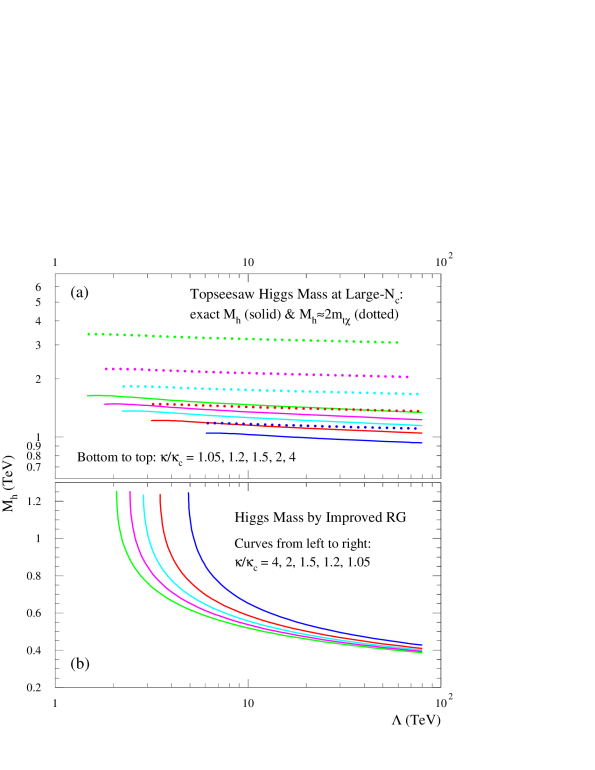
Figure 68: The predicted mass spectrum of the Top Seesaw Higgs boson: (a) by the large-$N_{c}$ fermion-bubble calculation; and (b) by an improved RG analysis including the Higgs self-coupling evolution.

In Fig. 69, we give the complete $S$ and $T$ contributions from the minimal Top Seesaw model, including corrections from both the composite Higgs boson and the seesaw quarks, and compare them with the 95% C.L. contour for $S-T$. Each figure corresponds to a different choice of critical coupling, $\kappa/\kappa_{c}$, and shows the trajectory in the $S-T$ plane as the $\chi$ mass varies. The results are based on both the large-$N_{c}$ fermion-bubble calculation and an improved RG in ref.[468]. The improved RG approach gives lower Higgs mass values (around $400-500$ GeV) so that the curves are slightly shifted towards the upper left (the reality is somewhere between these two trajectories). The figure clearly illustrates that the Top Seesaw model is consistent with the electroweak precision data provided $M_{\chi}$ is in the appropriate mass range. For instance, when the Topcolor force is slightly super-critical, we see that precision data are effectively probing $M_{\chi}\sim 4$ TeV. In Fig. 70, we display the same $S-T$ trajectories as in Fig. 69, but with the corresponding Higgs mass ($M_{h}$) values marked [468].

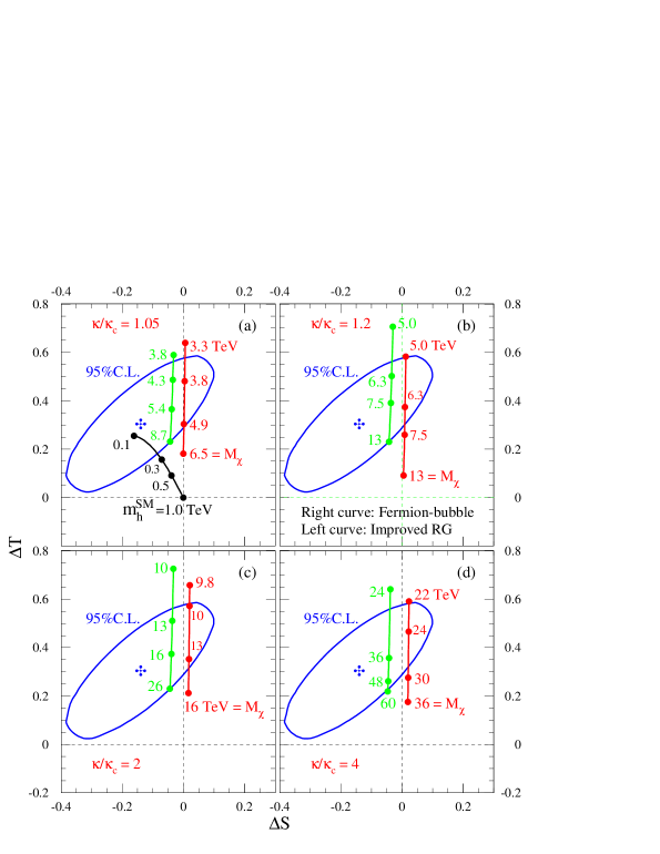
Figure 69: Top Seesaw contributions to $S$ and $T$ are compared with the 95% c.l. error ellipse (with $m_{h}^{\rm ref}=1$ TeV) for $\kappa/\kappa_{c}=1.05,\,1.2,\,2,\,4$, shown as a function of $M_{\chi}$. In each plot, the curve on the right is derived from the large-$N_{c}$ fermion bubble calculation, the curve on the left is deduced by an improved RG approach. For reference, the SM Higgs corrections to ($S$, $T$), relative to $m_{h}^{\rm ref}=1$ TeV, are given for $m_{h}^{\rm SM}$ varying from 100 GeV up to 1.0 TeV in plot (a). (from Hill, He and Tait [468]).

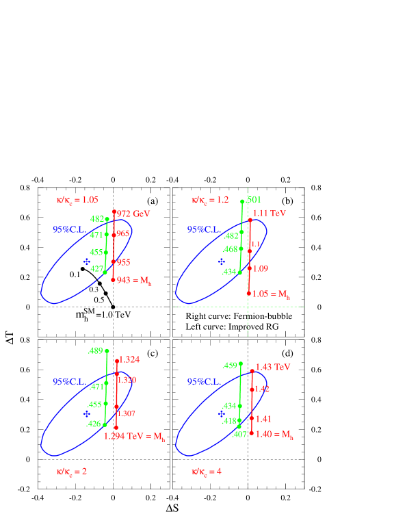
Figure 70: Same as Fig. 69, but with the corresponding $M_{h}$ values marked on the $S$-$T$ trajectories instead. (from Hill, He and Tait [468]).

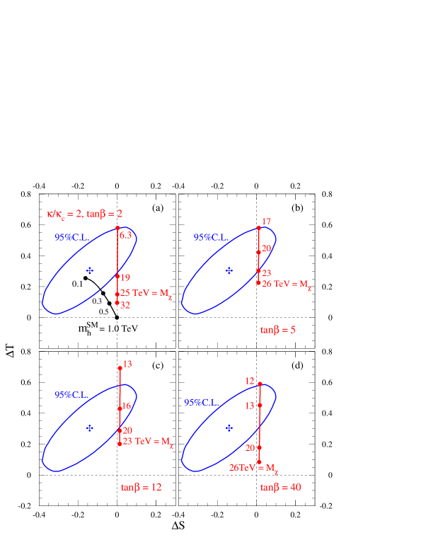
Figure 71: Top and bottom seesaw contributions to $S$ and $T$ are compared with the 95% C.L. error ellipse (with $m_{h}^{\rm ref}=1$ TeV) for $\kappa/\kappa_{c}=2$ and $\chi=3\times 10^{-3}$ with a variety of values of $\tan\beta$. The $S$-$T$ trajectories (including both Higgs and quark contributions) are shown as a function of $M_{\chi}$. For reference, the SM Higgs corrections to ($S$, $T$), relative to $m_{h}^{\rm ref}=1$ TeV, are depicted for $m_{h}^{\rm SM}$ varying from 100 GeV up to 1.0 TeV in plot (a).

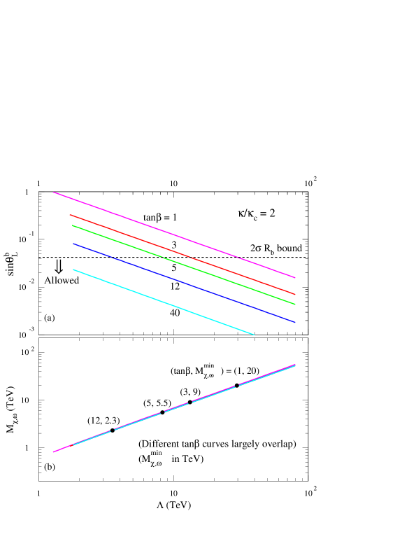
Figure 72: The $R_{b}$ limits are shown for the $b$ seesaw angle $s_{L}^{b}=\sin\theta_{L}^{b}$ in plot (a) and for the mass $M_{\omega}(\simeq M_{\chi})$ in plot (b). Here, we choose $\kappa/\kappa_{c}=2$ and a wide range of $\tan\beta$ values.

The inclusion of a bottom seesaw generates additional $b$-$\omega$ mixing ($\omega\equiv b^{H}$ is the seesaw partner of $b$) which makes nontrivial contributions to the $S$ and $T$ parameters and also to the $Z\rightarrow\bar{b}b$ vertex. Furthermore, the composite Higgs sector now contains two doublets and thus provides additional corrections to the precision observables. The $b-\omega$ mixing induces a positive shift in the left-handed $Z$-$b$-$\bar{b}$ coupling,

$$\delta g_{L}^{b}=+\frac{e}{2\sin\!\theta_{W}\cos\!\theta_{W}}(\sin\phi_{b})^{2}\,,$$ (4.203)

which results in a decrease of $R_{b}=\Gamma[Z\to b\bar{b}]/\Gamma[Z\to{\rm hadrons}]$, i.e., $R_{b}\simeq R_{b}^{\rm SM}-0.39(s^{b}_{L})^{2}$, as obtained in Ref. [464, 468]. This puts an upper bound on the $b$-seesaw angle,

$$\sin\phi_{b}~{}\simeq~{}\frac{m_{b}/\mu_{\omega}}{\sqrt{1+r_{b}}}~{}\simeq~{}\frac{m_{b}}{M_{\omega}\sqrt{r_{b}}}\,,$$ (4.204)

and correspondingly a lower bound on the mass $M_{\omega}$ ($\simeq M_{\chi}$), as summarized in Fig. 72. The $R_{b}$ bound will mainly constrain the low $\tan\beta$ region of the effective composite two doublet model.

Variant models [417, 467] in which vectorial weak-doublet partners exist for both top and bottom give similar contributions to $T$ as the models with a weak-singlet partner for top, while the contributions to $R_{b}$ are suppressed by a small mixing angle. The lower bound on these exotic quarks is, then, of order a few TeV, assuming they are degenerate. In principle, one could experimentally distinguish between the models with weak-singlet and weak-doublet mixings by measuring $A^{t}_{LR}$ at an NLC [467]. The predicted shifts relative to the SM value would be of similar size but opposite sign, as the $Zt_{L}t_{L}$ coupling is altered in the weak-singlet models while the $Zt_{R}t_{R}$ coupling is altered in the weak-doublet models.

As discussed in [470], it is possible to use existing Tevatron data to set limits on direct production of the $\chi$-like states. New, mostly-singlet, quarks decaying via mixing to an ordinary quark plus a W boson would contribute to the dilepton events used by the CDF [471] and D0 [472] experiments to measure the top quark production cross-section. Since the weak-singlet quarks are color triplets, they would be produced with the same cross-section as sequential quarks of identical mass. However the weak-singlet quarks can decay via neutral-currents (e.g. $d^{H}\to Zd^{L}$) as well as charged-currents (e.g. $d^{H}\to Wu^{L}$), and this lowers the branching fraction of the produced quarks to the final states to which the search is sensitive. In fact, the decay width $b^{H}\to c^{L}W$ is so strongly suppressed both by Cabbibo factors and the large rate of $b^{H}\to b^{L}Z$, that the Tevatron data do not provide a lower bound on $M^{H}_{b}$. For models in which all quarks have weak-singlet partners, the limits

$$M^{H}_{d,s}>\left\{\ {153\ {\rm GeV}\ \ \ {\rm CDF}}\atop{143\ {\rm GeV}\ \ \ {\rm D0}}\right\}$$ (4.205)

Similarly, mass limits on new mostly-singlet leptons (for flavor-universal mixing models) can be extracted from the results of LEP II searches for new sequential lepton doublets. In the relevant searches, the new neutral lepton $N$ is assumed to be heavier than its charged partner $L$ and $L$ is assumed to decay only via charged-current mixing with a Standard Model lepton (i.e. $BR(L\to\nu_{\ell}W^{*})=1.0$). The OPAL [473] and DELPHI [474] experiments have each set a 95% c.l. lower bound of order 80 GeV on the mass of a sequential charged lepton. As detailed in [470], when one adjusts for the increased production rate and decreased charged-current branching fraction of the mostly-singlet $\ell^{H}$ states, the resulting limit is

$$M^{H}_{\ell}\geq 84.9{\rm GeV}\ .$$ (4.206)

is slightly stronger.

Finally, CDF limits [475] on heavy $b^{H}$ quarks pair-produced through QCD processes and decaying via neutral currents can be applied to the weak-singlet fermions so long as the value of $B(b^{H}\to b^{L}Z^{0})$ is included. CDF finds 95% c.l. upper limits on the product of cross-section and squared branching fraction as shown in figure 73. For $B(b^{H}\to b^{L}Z^{0})=100\%$, heavy quarks with masses between 100 and 199 GeV are excluded. But if the neutral-current branching fraction decreases for heavier $b^{\prime}$ quarks, as in the models discussed in [470], $b^{\prime}$ quarks as light as 160 GeV may still be allowed by the data.

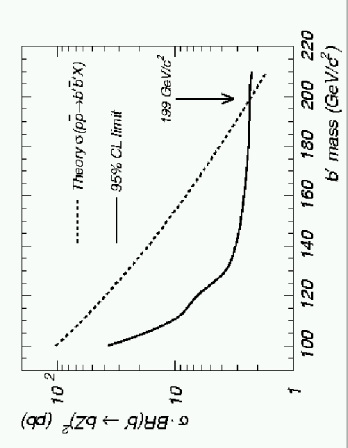
Figure 73: The 95% c.l. upper limit on $p\bar{p}\to b^{\prime}\bar{b}^{\prime}X$ production cross section times the $b^{\prime}\to bZ$ branching ratio squared (solid). The dashed curve shows the value predicted in a theory where the branching ratio is 100% [475].

Ultimately, at higher-energy hadron colliders, direct pair-production of the $\chi$ states and their subsequent decay via $\chi\rightarrow ht\rightarrow t\bar{t}t$ could yield [468], a spectacular $6t$ final state. As shown in Fig. 74, the cross section for this process with $m_{\chi}=1$ TeV would be $\sim 10$ pb.

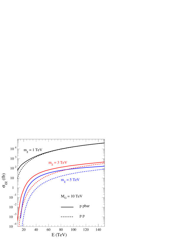
Figure 74: Cross-section for pair production of $\chi$ states at high energy hadron colliders, leading to 6-top events [194].

4.5.2 Flavorons

As an extension of the Top Seesaw mechanism, models with flavor universal dynamical symmetry breaking have been proposed [466, 476]. In these models, the dynamics are driven by family or large flavor gauge symmetries; when these symmetries break, multiplets of heavy “flavoron” bosons remain in the specrum. Their masses, like the symmetry breaking scale, are expected to be of order a few TeV. The flavorons’ couplings to fermions must be strong enough to generate condensates that break the electroweak symmetry and provide the ordinary fermions with masses. As a result, the flavorons tend to be readily produced at hadron colliders like the Tevatron – but also to have large decay widths that make their detection in dijet invariant mass spectra a challenge [466].

For the moment, some of the best limits on flavor gauge bosons come from precision electroweak data [454]. Flavorons coupling to ordinary fermions can give rise to direct corrections to $Zff$ vertices; generally speaking, if the $Zff$ coupling is $g_{f}$, the correction is [429]

$$\Delta g_{f}=g_{f}\frac{G\kappa_{F}}{6\pi}\frac{M_{Z}^{2}}{M_{F}^{2}}\ln\left(\frac{M_{F}^{2}}{M_{Z}^{2}}\right)$$ (4.207)

where $G$, $\kappa\equiv g_{F}^{2}/4\pi$, and $M_{F}$ are the group theory factor, coupling, and mass appropriate to the particular flavouron. Flavoron exchange across $t$ and $b$ quark loops will generally contribute to the $T$ parameter an amount (in leading log)

$$T=N_{c}(G^{\prime}_{LL}+2G^{\prime}_{RR})\frac{\kappa m_{t}^{4}}{32\pi^{2}\sin^{2}\theta_{W}\cos^{2}\theta_{W}M_{Z}^{2}M_{F}^{2}}\left[\ln(M_{F}^{2}/m_{t}^{2})\right]^{2}$$ (4.208)

where $G^{\prime}_{LL,RR}$ are group theory factors for flavoron couplings to left-handed and right-handed quarks. In addition, in models in which some generator of the flavor group mixes with hypercharge or the diagonal generator of $SU(2)_{W}$, the associated $Z-Z^{\prime}$ mixing also contributes to $T$.

For each of the three representative flavoron models mentioned here, we assume that flavoron exchange at low energies may be treated in the NJL approximation (with four-fermion coupling $4\pi\kappa/2\!M_{F}^{2}$). The critical coupling required for chiral symmetry breaking is

$$\kappa_{crit}=\frac{2N\pi}{N^{2}-1}.$$ (4.209)

The minimal model [466, 476, 477, 83] has a gauged SU(3) family symmetry acting on the left-handed quark doublets. This family symmetry group does not mix with the Standard Model gauge groups and the model leaves the GIM mechanism intact. The critical coupling is $\kappa_{crit}=2.36$. Models in which the $SU(9)$ symmetry of color and family multiplicity of the left-handed quarks is gauged [466, 265] also preserve GIM. A proto-color group acting on the right-handed quarks is also present; obtaining the correct value for $\alpha_{s}$ in its presence requires

$$\kappa\geq 3\alpha_{s}(2\rm{TeV})\approx 0.3$$ (4.210)

Ignoring mixing between the flavor and proto-color group generators, the critical coupling for chiral symmetry breaking is $\kappa_{crit}=0.71$. If the full $SU(12)$ flavor symmetry of all the left-handed quark and lepton doublets is gauged [466, 265], both a proto-color group and a proto-hypercharge group must be included for the right-handed fermions, and the constraint (4.210) still applies. In this case, $\kappa_{crit}=0.53$ – not far above the lower limit. The 95% c.l. lower bound on $M_{F}$ from precision electroweak data for $\kappa$ at its critical value is approximately 2 TeV for all three models [454].

Comparable limits on $M_{F}$ (for critical coupling $\kappa$) in the $SU(3)$ and $SU(9)$ models have been obtained from Tevatron Run I data [478]. Run II should be sensitive to $M_{F}$ up to 2.5 - 3 TeV with 2 $fb^{-1}$ of data. For the $SU(3)$ model, both dijet and anomalous single top production are likely to yield large signals; in the SU(9) model, the dijet signal is relatively enhanced and the single top signal, relatively reduced in size, enabling the two models to be distinguished if both channels are studied.

A significantly stronger bound on the flavorons of the $SU(12)$ model derives from atomic parity violation: $M_{F}\begin{array}[]{c}\,\sim\vspace{-21pt}\\ >\end{array}10$ TeV [478]. Flavorons from the $SU(12)$ model light enough to produce visible signals at the Tevatron are already excluded by this limit.

4.6 Extra Dimensions at the TeV Scale

Recently there has been considerable interest in theories of extra dimensions of space which emerge not far from the weak scale. We cannot give a comprehensive review of this burgeoning field, but we will outline some key ideas relating to electroweak symmetry breaking and the physics of new strong dynamics. The ideas largely stem from the view that string theories admit an arbitrary hierarchy between the compactification scale of the extra dimensions, and the fundamental string scale. Moreover, with gravity in a higher dimensional bulk the “true” Planck scale can emerge as a $\sim 100$ TeV scale, but is subject to rapid power-law renormalization; grand unification remains viable in these theories, and one is led to a long list of novel phenomena.

Some of the key early works are those of Antoniadis, et al. and Lykken (weak scale superstrings [479, 480],[481]); Arkani-Hamed, Dimopoulos, and Dvali, (millimeter scale gravity [482, 483]); Dienes, Dudas and Gherghetta, (gauge fields in the bulk and power-law unification [484, 485]); Randall, Sundrum (DeSitter space in the bulk and natural hierarchy [486, 487]). It is also essential that chiral fermions emerge in the compactified theory, and this is possible by implementing orbifold compactification ala Horava and Witten, [488], or domain walls ala Arkani-Hamed and Schmaltz [489]. In the latter case dynamical mechanisms arise for the origin of generational hierarchies, and the CKM matrix. [490, 491] Many phenomenological constraints have been placed upon the scales of the new extra dimension(s), and many variations and developments of this theme now exist, too numerous to review here. A compactification scale lower limit of order $\sim 1$ TeV seems to be indicated phenomenologically.

Why not consider extra space-time dimensions at the weak scale? After all, supersymmetry is an extra-dimensional theory in which the extra dimensions are fermionic, or Grassmanian, variables. Supersymmetry leads naturally, upon “integrating out” the extra fermionic dimensions (i.e., descending from a superspace action to a space-time action), to a perturbative extension of the Standard Model, e.g., the MSSM. In such a scheme the Higgs sector is at least a two-doublet model, and the lightest Higgs boson is expected to be in a range determined by the perturbative electroweak constraints, $\mathrel{\vbox{\hbox{$<$}\nointerlineskip\hbox{$\sim$}}}140$ GeV. ¿From a “bottom-up” perspective the key lesson from Supersymmetry is that an organizing principle for physics beyond the Standard Model emerges from hidden extra dimensions which are then integrated out. Upon specifying the algebraic properties of the extra dimensions one is led to a particular symmetry structure and class of dynamics for EWSB. The particular extra dimensions in which we will be interested are ordinary c-numbers, but one can contemplate other possibilities [492, 493, 494].

Extra dimensions do not show up as new “real estate,” but rather they appear in accelerator experiments as new particles . These are the excited modes of existing fields, e.g., quarks, leptons, gauge bosons, the graviton, that propagate in the compact extra dimensions, and are known as Kaluza-Klein (KK) excitations. The KK modes typically appear as a ladder spectrum of discrete resonances with the same quantum numbers as the zero-mode field itself. For example, if we consider the possibility that QCD gauge fields (gluons) can propagate in the bulk then the KK modes show up as a sequence of massive colorons.

The idea of extra c-number dimensions near the weak scale has led to the proposal of dynamical schemes that can imitate the strong dynamics we have discussed in this review. Dobrescu first observed that the main ingredients of Topcolor, i.e., the colorons, appear naturally as KK modes of the gluon [496] and a number of detailed models have been discussed [497, 498, 499, 500]. These essentially follow the idea of top condensation as discussed in Section 4. The other key ingredient of the Top Seesaw model, the seesaw partner $\chi$ quarks, can emerge as KK modes as well.

4.6.1 Deconstruction

As KK-modes begin to appear in accelerator experiments, we can ask: “how are they to be described phenomenologically, as if we have no knowledge of the extra dimensions themselves?” or, equivalently, “What is the effective low energy Lagrangian of the KK modes?” This has led to a new twist in the development of these models known as “deconstruction.” Independently, the “Harvard” group of Arkani-Hamed, Cohen and Georgi, [42, 501, 502] and the “Fermilab” group Hill, Pokorski, Wang and Cheng [41, 503, 504], have proposed using a lattice to describe the extra dimensions. The $3+1$ dimensions of space-time are continuous, while the extra compact dimensions are latticized (this is known as a “transverse lattice” [505]). By using the lattice technique, one can “integrate out” the extra dimensions, preserving local gauge invariance, and arrive at a manifestly gauge invariant effective Lagrangian including Kaluza-Klein modes (in a sense the KK modes are analogues of superpartners).

To get a flavor for deconstruction, let us consider the first KK-mode excitation of the gluon in a compactified theory of $D=4+1$ dimensions. We can write its effective Lagrangian knowing only the $SU(3)$ symmetry of QCD. The lowest KK mode appears as a “coloron,” a heavy linear octet representation of the gauge group $SU(3)$; its mass is the only parameter determined by compactification. A heavy vector meson which forms a multiplet under a (local or global) symmetry group $G$, can always be described as a gauge field [163], with a spontaneously broken gauge group that is an identical copy of $G$. For the single coloron case we have $G=SU(3)$. Hence, we may take our theory of a gluon plus its first excitation to be based upon the gauge group $G^{\prime}=SU(3)_{1}\times SU(3)_{2}$ and break this to $G=SU(3)$ with a Higgs field $\Phi$ transforming as a $(3,\bar{3})$.

By constructing a Higgs potential:

$$V(\Phi)=-M^{2}\mathop{\rm Tr}(\Phi^{2})+\lambda\mathop{\rm Tr}(\Phi^{4})+\lambda\mathop{\rm Tr}(\Phi^{2})^{2}+M^{\prime}\det(\Phi)$$ (4.211)

we can arrange for $\Phi$ to develop a vacuum expectation value $V$, by which all unwanted Higgs degrees of freedom are elevated to the large mass scale $\propto M$. Note that in trying to discard the extra $10$ degrees of freedom in $\Phi$ as a Higgs field, we encounter a unitarity bound [24, 506, 507] which predicts the string scale from $M$.

The Lagrangian containing the gluon and the first KK mode is therefore:

$${\cal{L}}=-\frac{1}{4}F^{A}_{1\mu\nu}F_{1}^{A\mu\nu}-\frac{1}{4}F^{A}_{2\mu\nu}F_{2}^{A\mu\nu}+|D_{\mu}\Phi|^{2}-V(\Phi).$$ (4.212)

The field $\Phi$, after developing a VEV, and decoupling the Higgs degrees of freedom, can be parameterized by a chiral field:

$$\Phi\rightarrow V\exp(i\phi^{A}T^{A}/\sqrt{2}V)$$ (4.213)

This is exactly the structure that would emerge from a Wilson lattice with two transverse lattice points (which are now “branes, each carrying a $3+1$ theory). We also see that this is identical to the gauge sector of Topcolor models. With the breaking in place, the theory has two mass eigenstates, the gluon and coloron:

$$G_{\mu}^{A}=\cos\theta A_{1\mu}^{A}+\sin\theta A_{2\mu}^{A};\qquad\qquad B_{\mu}^{A}=-\sin\theta A_{1\mu}^{A}+\cos\theta A_{2\mu}^{A};$$ (4.214)

where $A_{i\mu}$ belongs to $SU(3)_{i}$. If we allow $SU(3)_{i}$ to have a coupling constant $g_{i}$ then we find:

$$\tan\theta=\frac{g_{1}}{g_{2}}$$ (4.215)

The mass of the coloron is given by

$$M_{K}=V\sqrt{g_{1}^{2}+g_{2}^{2}}=\frac{1}{R}$$ (4.216)

where $R$ is identified with the radius of the compactified extra dimension. We also see that the low energy QCD-coupling is related to $g_{i}$ as:

$$\frac{1}{g_{QCD}^{2}}=\frac{1}{g^{2}_{1}}+\frac{1}{g^{2}_{2}}$$ (4.217)

With $g_{1}=g_{2}$ we have $g_{1}^{2}=2g_{QCD}^{2}$ and this is the onset of “power-law running” of the coupling constant. The model indeed represents a single KK mode, descending from higher dimensions. Conversely, observation of a coloron in the particle spectrum could be taken to suggest that a new extra dimension is opening up.

Figure 75: Dirac fermion corresponding to constant $\phi$ has both chiral modes on all branes. The $\times$’s denote the $\phi$ couplings on each brane, and the links are the latticized fermion kinetic terms which become Wilson links when gauge fields are present. (from [508]) The spectrum here has a singlet lowest massive mode, and doubled KK modes; by adding a Wilson term one can remove one of the two cross-bars between adjacent branes, and elminate second Brillouin zone doubling in the spectrum.

Figure 76: A chiral fermion occurs on brane $n$ where $\phi(x^{5})$ swings rapidly through zero. The chiral fermion has kinetic term (Wilson links) connecting to adjoining branes. (from [508])

Figure 77: Pure top quark condensation by Topcolor is obtained in the limit of critical coupling on brane $n$ and decoupling to the nearest neighbors. Decoupling corresponds to taking the compactification mass scale large; the links are then denoted by dashed lines. (from [508])

The full lattice description of QCD is a straightforward generalization of this model [41]. If we consider the full lattice gauge theory in $4+1$ dimensions with a Wilson action for the extra dimension, we obtain the Lagrangian:

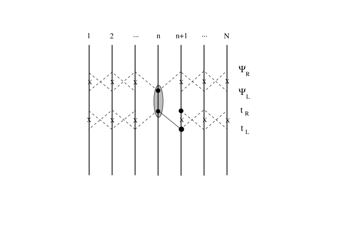
Figure 78: Top Seesaw Model arises when the effects of nearest neighbor vectorlike fermions are retained, i.e., when these heavier states are only partially decoupled. Keeping more links maintains the seesaw. Usually we denote $t_{Rn}\sim\chi_{R}$, $t_{Ln+1}\sim\chi_{L}$, $t_{Rn+1}\sim t_{R}$. (from [508])

$${\cal{L}}=-\frac{1}{4}\sum_{j=1}^{N}F^{A}_{j\mu\nu}F_{j}^{A\mu\nu}+\sum_{k=1}^{N-1}\mathop{\rm Tr}(D_{\mu}\Phi_{k})^{2}$$ (4.218)

Here there are $N-1$ $\Phi$ fields, and the $kth$ field transforms as an $(3_{k},\bar{3}_{k+1})$ representation, straddling the nearest neighbor $SU(3)_{k}$ and $SU(3)_{k+1}$ gauge groups. $\Phi_{k}$ is a unitary matrix, and represents the Wilson line:

$$\Phi_{k}=V\exp\left(ig\int_{x_{k}}^{x_{k+1}}dx^{5}A_{5}^{a}T^{a}\right)$$ (4.219)

$\Phi_{k}$ may be parameterized by:

$$\Phi_{k}=V\exp(i\phi_{k}^{a}T^{a}/\sqrt{2}V)$$ (4.220)

where $T^{a}=\lambda^{a}/2$. This clearly matches our previous discussion of a single KK mode.

The $\Phi_{k}$ kinetic terms imply a gauge field mass term of the form:

$$\frac{1}{2}g^{2}V^{2}\sum_{k=1}^{N-1}(A^{a}_{k\mu}-A^{a}_{(k+1)\mu})^{2}$$ (4.221)

Performing the mass spectrum analysis of the model is equivalent to analyzing the phonon spectrum of a one-dimensional crystal lattice. The mass term is readily diagonalized and we obtain eigenvalues reflecting a ladder of states with:

$$M_{n}=\sqrt{2}gV\sin(\pi n/2N)$$ (4.222)

the lowest energy masses given by:

$$M_{n}\approx\pi gVn/N\sqrt{2}\equiv\frac{1}{R}$$ (4.223)

This is the spectrum assuming free boundary conditions on the lattice and corresponds to orbifolding. With periodic boundary conditions instead, one gets the $A_{5}^{a}$ as low energy modes as well, which act like pseudo-scalars, and the KK mode levels are doubled.

The net result is that the effective Lagrangian for, e.g., QCD propagating in the extra dimensional bulk, is a chain of gauge groups of the form: $SU(3)\times SU(3)\times SU(3)\times...$, one gauge group per lattice brane. The high energy coupling constant common to each group is $g\sim\sqrt{N}g_{QCD}$, consistent with the power-law running. ¿From a “bottom-up” perspective, one writes down this gauge structure with arbitrary relevant operators with arbitrary coefficients to describe the most general low energy effective theory for extra-dimensional physics.

Various additional dynamical issues in deconstructed theories are currently under investigation, such as chiral dynamics [509, 510], electroweak observables [511, 512], unification [502, 513] and GUT breaking [514]. A number of authors have applied deconstruction to supersymmetric schemes and SUSY breaking [515, 516] [517, 518]. There are interesting and novel topological issues in the presence of many gauge factor groups, e.g., [519, 520]. Duality and supersymmetry can have an intriguing interplay [521] in these schemes via topology. Deconstructing gravity is in need of elaboration, but Bander has made an interesting first attempt in the language of vierbeins [522].

Fermions can be accomodated, and chirality can be engineered. Chiral fermions can be localized in the fifth dimension by background fields [489, 523, 524]. A free fermion has the continuum and latticized action (we neglect the gauge interactions here, and do not include Wilson terms):

$$\int d^{5}x\;\bar{\Psi}(i\partial\!\!\!/\!\,\,-\partial_{5}\gamma^{5}-\phi(x^{5}))\Psi\rightarrow\sum_{n=1}^{N}\int d^{4}x\;\bar{\Psi}_{n}(i\partial\!\!\!/\!\,\,-\phi_{n})\Psi_{n}+V\bar{\Psi}_{n}\gamma_{5}\Psi_{n+1}+h.c.$$ (4.224)

If the background field is approximately constant both chiral components of the fermion appear on each lattice brane, as depicted in Fig.(75). The cross bars are the latticized links allowing hopping of the fermion from $n$ to $n+1$ in eq.(4.224) If $\phi(x^{5})$ swings through zero rapidly in the vicinity of brane $n$, i.e., $\phi_{n}=0$ then only a single chiral component is normalizeable in the vicinity of $n$ and one gets a dislocation in the lattice as shown in Fig.(76).

The coupling strength of $SU(3)_{n}$ on the $n$-th brane will generally be renormalized by the dislocation and can become supercritical, Fig.(77). It would, therefore, not be coincidental to expect this to happen; indeed a variety of effects are expected to occur near the dislocation, e.g., the chiral fermions themselves can feed-back onto the gauge fields to produce such renormalization effects. The result is a chiral condensate on brane $n$ forming between chiral fermions. Identify $\Psi=(t,b)_{L}$ and $t_{R}$ as the chiral zero-modes on brane $n$ of two independent Dirac fields in the bulk. In the limit that we take the compact extra dimension very small, the nearest neighbor links decouple at low energies. In this limit we recover a Topcolor model with pure top quark condensation.

In Fig.(78) we illustrate the case that some of the links to nearest neighbors are not completely decoupled. Again, this can arise from renormalizations due to background fields, or to warping [503, 504]. Thus the mixing with heavy vectorlike fermions occurs in addition to the chiral dynamics on brane $n$. In this limit we obtain the Top Quark Seesaw Model.

4.6.2 Little Higgs Theories

Recently another approach to electroweak symmetry breaking has been revived, inspired by deconstruction, in which the Higgs itself is a PNGB, [501]. This is actually an old idea, due to Georgi, Kaplan, and others (see, e.g. [525][526][527]). The novelty presently is that delocalization in an extra dimension (or the minimal deconstructed description of such) leads to a potentially softer scheme in which dangerous gauge loop quadratic divergences contributing to the Higgs boson (mass)² can be cancelled in one loop order. The resulting models bear some resemblance to the MSSM Higgs structure.

There are now a number of schemes, most notably the “minimal moose model,” [528] and $SU(5)/SO(5)$ model [529, 530], and the $SU(6)/SO(6)$ scheme [531]. We briefly describe the “minimal moose” scheme.

When we periodically compactify a higher dimension we find that there is, in the absence of loops, a massless mode corresponding to the zero-mode of $A_{5}^{a}$. For QCD this would appear in the effective lagrangian as a color octet of pseudoscalars. However, since these modes carry color, they will acquire mass $\sim gV$. Arkani-Hamed, Cohen and Georgi show how this leads to a Coleman-Weinberg potential for the modes, and is generally finite. The authors then construct a scheme [501] in which this mode can arise as an electroweak isodoublet.

The idea, from a lattice point of view, is to latticize two compact dimensions with toroidal boundary conditions ($T_{2}$, the surface of a doughnut). The minimal plaquette action is then a generalized Eguchi-Kawai model [532], but with the additional links associated with the periodicity. At three of the four sites of the plaquette one attaches $SU(3)$ gauge groups. On the fourth cite one attaches $SU(2)\times U(1)$. The Wilson links (linking Higgs) which attach the $SU(2)\times U(1)$ gauge group to nearest neighbor $SU(3)$’s then contain components which transform as $I=\frac{1}{2}$ Higgs fields. The Coleman-Weinberg potential produces an unstable vacuum. The theory leads to an effective two-Higgs doublet model. The gauge couplings would be expected to raise the mass of the lightest Higgs to order $\sim g_{2}^{2}\Lambda^{2}$, but the discrete symmetries of the model, associated with the delocalized structure, lead to a GIM-like cancellation of this contribution. The dangerous term does occur at two-loop level $\sim g_{2}^{4}\Lambda^{2}$. With $\Lambda\sim 10$ TeV the scale of the “compactification dynamics” the lightest $0^{+}$ Higgs can be of low mass, $\sim 120$ GeV. Hence a “little” hierarchy, $10$ TeV $\mathrel{\vbox{\hbox{$<$}\nointerlineskip\hbox{$\sim$}}}\mu\mathrel{\vbox{\hbox{$<$}\nointerlineskip\hbox{$\sim$}}}$ $v_{weak}$ is protected in this scheme.

These models are receiving fuller elaboration at present. For a critical discussion of this scheme see K. Lane [533]. Two recent works attack several aspects of the models from the perspective of consistency with electroweak radiative corrections [534]. The models contain ingredients, such as $I=0$ PNGB’s, that develop tadpole VEV’s and may violate $T$ cosntraints. Also, the models such as $SU(5)/SO(5)$ employ a top seesaw to give to the top quark mass, and the extended fermion structure can be problematic in loops [535]. Some recent papers examine collider phenomenology of these schemes [536, 537].

Much remains to be done with Little Higgs schemes, in particular in establishing their phenomenological naturalness.

5 Outlook and Conclusions

The next decade will bring great discoveries in the field of elementary particle physics. The Tevatron Run-II program and the LHC will begin to reveal the mechanism(s) responsible for the origin of mass. The Large Hadron Collider in concert with a Linear Collider can begin detailed studies of the fields involved in electroweak symmetry breaking. In the longer term, a Very Large Hadron Collider will have the power to probe the corollary mechanisms that underlie the physics of flavor.

This review has focused on the possibility that the origin of mass involves a new strong dynamics near the TeV scale. As we have argued here, dynamical electroweak symmetry breaking, whether it comes in the guise of Technicolor, Topcolor, or some variant scheme, can provide a natural explanation for the weak scale. It can also provide tantalizing clues about the magnitudes and origins of the fermion masses and mixings, and may be able to explain CP violation. Indeed, many issues of flavor physics that are relegated to the Planck or Gut scale in perturbative theories, such as the MSSM, become accessible to sufficiently energetic accelerators in the dynamical framework.

Technicolor was created in the era in which the $W$ and $Z$ bosons are heavy and all known fermions are comparatively light. In the first approximation, therefore, the fermions are massless and Technicolor is essentially a pure QCD-like theory which naturally generates the weak scale, in analogy to the way the strong scale is generated by QCD through its “running coupling constant.” By itself, Technicolor requires a new gauge group and additional fermions, i.e., techniquarks. Technicolor is, however, an incomplete theory. Extended Technicolor was introduced to accomodate light fermion masses, but even the charm quark begins to push the limits on ETC from rare decay processes. Hence, one is led to various schemes to accomodate heavier fermion masses, such as Walking Technicolor and Multi-Scale Technicolor. Combinations with Supersymmetry and Bosonic Technicolor have been considered.

In the post–1990 era, in addition to the heavy $W$ and $Z$, we have the very heavy top quark. This leads to an alternate point of departure for dynamical models of EWSB, based on the idea of Topcolor. Topcolor by itself is a fine-tuned theory in which the top quark alone condenses, predicting $m_{t}\sim 220$ GeV, and this first–order theory can be ruled out. However, in concert with Technicolor, we arrive at viable models in which a new Techni-dynamics can coexist and the top quark acquires a dynamical mass through Topcolor. Such models, “Topcolor Assisted Technicolor” or TC2, predict a rich phenomenology that may be accessible to the Tevatron, and certainly to the LHC. In this view, the top quark is playing the role of the first techniquark.

Topcolor by itself, with a small extension, can naturally yield a completely viable theory of dynamical EWSB: the “Top Quark Seesaw.” In this scheme the top quark condenses, through strong Topcolor, but there are additional vectorlike fermions that mix to give the physical mass of the top quark through a seesaw. The Top Quark Seesaw, despite an effective boundstate Higgs boson with a mass of $\sim 1$ TeV, is in agreement with present oblique radiative corrections (the $S-T$ plot). It explains the $W$ and $Z$ masses, as well as $m_{t}$ and $m_{b}$, the latter through instantons or a simple extension. Moreover, it involves the fairly robust gauge group imbedding of QCD to $SU(3)\times SU(3)$ and additional vectorlike fermions, and is therefore as economical as Technicolor. Finally, the $SU(3)\times SU(3)$ structure, and the new vectorlike fermions, are completely natural ingredients expected from extra dimensions of space near the weak scale. The model may be extendable to generate all known fermion masses and mixing angles, though no complete theory has yet been written down.

Thus, strong dynamical models of EWSB have evolved and remain viable and consistent with all known experimental limits. Of course, regardless of the theoretical beauty of any given scenario, its validity will ultimately be ascertained through experiment. Should the slight discrepancies in the electroweak precision tests, e.g., the forward-backward asymmetries of leptons and hadrons, open into a new phenomenology, then novel TeV-scale dynamics may be in the offing. Should the hadron colliders find a spectrum of new states with unexpectedly large production cross-sections, or should the Higgs boson be shown to be very heavy through exclusion, then new strong dynamics will be indicated.

We have seen that new strong dynamics can be consistent with the presence of (even weak-scale) Supersymmetry. Another exciting candidate system of organizing principles is the existence of c-number extra dimensions, which we have found to be naturally associated with several types of strong dynamics, such as the Top Seesaw or the Little Higgs models. Hence, we will likely uncover new fundamental organizing principles in our quest to unravel EWSB, whether the dynamics is perturbative or strongly coupled.

The task of theorists is to prepare to understand whatever results emerge from the upcoming experiments aimed at the electroweak scale. In this review we have focused upon a set of ideas complementary to the most popular and well-studied perturbative MSSM scenarios. We have seen that, when considered in equivalent detail, these dynamical theories are no less viable, given current experimental bounds. They hint at connections to deeper ideas about the structure and interplay of space, time and matter. They remain, in our opinion, exciting prospects for discovery in the near future.

6 Acknowledgements

We wish to thank the following individuals for useful input and commentary to this review: Tom Appelquist, William Bardeen, Gustavo Burdman, Sekhar Chivukula, Bogdan Dobrescu, Estia Eichten, Keith Ellis, Hong-Jian He, Ken Lane, Chris Quigg, and Koichi Yamawaki.

Appendix A: The Standard Model

A(a) Summary of Standard Model Structure

The Standard Model is a unified description of the electromagnetic and weak interactions based upon the gauge group $SU(2)\times U(1)$. The fermions are chiral, i.e., the left-handed fermions are doublets with respect to the $SU(2)$ gauge group, while the right-handed fermions are singlets. Left– and right–handed fermions also carry different charges under the $U(1)$ gauge group.

The concept of spontaneous symmetry breaking, to provide both the gauge boson and fermion masses, is necessarily imbedded into the Standard Model. As in the Landau-Ginzburg superconductor, a scalar field, the “Higgs field,” is introduced explicitly, “by hand,” to provide the symmetry breaking condensate. Recalling the toy model example of Section 1.3(iii), the fermions can only acquire Dirac masses (or neutrino Majorana masses) through coupling to the condensing Higgs boson, since explicit fermion mass terms are not singlets under the gauge group, owing to the fermionic chiral charge assignments. The gauge fields also acquire their masses through the condensing Higgs boson, as per the toy example of Section 1.3(iv).

We begin by considering an $SU(2)\times U(1)$ gauge theory with one scalar field that transforms as an isodoublet under the $SU(2)$ group. The covariant derivative for the theory is given by:

$$iD_{\mu} = i\partial_{\mu}-g_{2}W_{\mu}^{a}{Q^{a}}-g_{1}B_{\mu}\frac{Y}{2}$$ (A.1)

$$= i\partial_{\mu}-g_{2}{W}_{\mu}^{+}Q^{-}-g_{2}{W}_{\mu}^{-}Q^{+}-g_{2}{W}^{3}_{\mu}Q^{3}-g_{1}{B}_{\mu}\frac{Y}{2}$$

where the “charge basis” expressions are $Q^{\pm}=(Q^{1}\pm iQ^{2})/\sqrt{2}$, and $W_{\mu}^{\pm}=(W_{\mu}^{1}\pm iW_{\mu}^{2})/\sqrt{2}$. Note there are two gauge coupling constants, $g_{2}$ and $g_{1}$, one for each simple subgroup of the theory. The $Q^{a}$ are the $SU(2)$ weak charges and $Y$ is the $U(1)$ hypercharge. The $Q^{a}$ satisfy the $SU(2)$ Lie algebra:

$$[Q^{a},Q^{b}]=i\epsilon^{abc}Q^{c}.$$ (A.2)

These charges are at this stage abstract operators, the generators of the associated groups. We specialize to particular representations for the charges, choosing an $I=\frac{1}{2}$ weak isospin representation for the left-handed fermions, and Higgs boson, in which $Q^{a}=\tau^{a}/2$ where the $\tau^{a}$ are Pauli matrices. The right-handed fermions are singlets, annihilated by the $Q^{a}$. We further define the weak hypercharge for any representation by its eigenvalue, $Y_{r}$, or the abstract operator $Y$.

In defining the Standard Model we choose a specific generator to correspond to the electric charge operator:

$$Q_{EM}=Q^{3}+\frac{Y}{2}$$ (A.3)

Note that the choice of $Q^{3}$ is a choice of basis, i.e., we could use any normalized linear combination of the $Q^{a}$ in place of $Q^{3}$, but by a gauge rotation we can always align that linear combination with $Q^{3}$. Given the electric charges of particles, this defines the $Y_{r}$ for any representation.

The Standard Model left-handed fermionic matter doublets are then assigned the following structure and weak hypercharges:

$$\left(\begin{array}[]{c}u^{2/3}\\ d^{-1/3}\end{array}\right)_{L},Y_{r}=\frac{1}{3};\qquad\;\left(\begin{array}[]{c}\nu^{0}\\ e^{-1}\end{array}\right)_{L},Y_{r}=-1;\qquad\;H^{c}=\left(\begin{array}[]{c}\phi^{+}\\ -\bar{\phi}^{0}\end{array}\right)\;Y_{r}={+1};$$ (A.4)

where the last entry is the “charge–conjugated Higgs field” defined by $H^{c}=i\tau^{2}H^{*}$. The right–handed fermions are $SU(2)$ singlets, i.e., $[Q^{a},\psi_{R}]=0$, hence,

$$u_{R}^{2/3},\;\;Y_{r}=\frac{4}{3};\qquad\;d_{R}^{-1/3},\;\;Y_{r}=-\frac{2}{3};\qquad\;e_{R}^{-1},\;\;Y_{r}={-2};\qquad\;\nu_{R}^{0},\;\;Y_{r}=0.$$ (A.5)

A right–handed neutrino is sterile, and usually omitted in the definition of the “Standard Model.”

Returning to the gauge bosons, if we write the linear combinations:

$$W_{\mu}^{3} = Z^{0}_{\mu}\cos\theta+A_{\mu}\sin\theta$$

$$B_{\mu} = -Z^{0}_{\mu}\sin\theta+A_{\mu}\cos\theta$$ (A.6)

where $Z^{0}_{\mu}$ ($A_{\mu}$) is the physical $Z$-boson (photon), then we see,

$$g_{2}\sin\theta=e;\qquad\qquad g_{1}\cos\theta=e;\qquad\qquad$$ (A.7)

The photon thus couples to $eQ_{EM}$ with strength $e$ where:

$$\frac{1}{e^{2}}=\frac{1}{g_{2}^{2}}+\frac{1}{g_{1}^{2}}$$ (A.8)

The weak mixing angle is defined by:

$$\tan\theta=\frac{g_{1}}{g_{2}}$$ (A.9)

The gauge covariant field strengths are defined by commutators of the covariant derivative:

$$F_{\mu\nu}^{a} = -\frac{i}{g_{2}^{2}}\mathop{\rm Tr}\left({\tau^{a}}[D_{\mu},D_{\nu}]\right)=\partial_{\mu}A^{a}_{\nu}-\partial_{\nu}A^{a}_{\mu}+\epsilon^{abc}A_{\mu}^{b}A_{\nu}^{c}$$

$$F_{\mu\nu} = -\frac{i}{g_{1}^{2}}Y_{r}^{-1}\mathop{\rm Tr}\left([D_{\mu},D_{\nu}]\right)=\partial_{\mu}B_{\nu}-\partial_{\nu}B_{\mu}$$ (A.10)

Then the gauge field kinetic terms are:

$${\cal{L}}_{G.B.\;kinetic}=-\frac{1}{4}F_{\mu\nu}^{a}F_{\mu\nu}^{a}-\frac{1}{4}F_{\mu\nu}F_{\mu\nu}$$ (A.11)

Consider the complex doublet scalar Higgs-boson with $Y_{r}=-1$:

$$H=\left(\begin{array}[]{c}\phi^{0}\\ \phi^{-}\end{array}\right)$$ (A.12)

The Lagrangian for $H$ takes the form:

$${\cal{L}} = (D_{\mu}H)^{\dagger}(D^{\mu}H)-V(H)$$ (A.13)

The masses of the gauge bosons are generated by spontaneous symmetry breaking, in strict analogy to the generation of mass in a superconductor as discussed in Section 1.3(iv). We assume that $V(H)$ has an unstable extremum for $H=0$ and a nontrivial minimum, e.g., we can write:

$$V(H)=\frac{\lambda}{2}(H^{\dagger}H-v_{weak}^{2})^{2}$$ (A.14)

The Higgs boson then develops a vacuum expectation value. This may, without loss of generality be taken in the upper component (which is, again, the choice of orientation within the internal $SU(2)$ space that defines the electric charge to be that combination of generators that annihilates $\left\langle H\right\rangle$):

$$\left\langle H\right\rangle=\left(\begin{array}[]{c}v_{weak}\\ 0\end{array}\right)\qquad\makebox{or:}\qquad{H}=\exp\left(i\frac{\pi^{a}\tau^{a}}{\sqrt{2}v_{weak}}\right)\left(\begin{array}[]{c}v_{weak}+\frac{h}{\sqrt{2}}\\ 0\end{array}\right)$$ (A.15)

In the present normalization $v_{weak}=(2\sqrt{2}G_{F})^{-1/2}=175$ GeV. Note that $Q_{EM}$ acting on the Higgs VEV is zero, which implies that the photon remains a massless gauge boson $\gamma$.

When we substitute the anzatz (A.15) into the Higgs boson kinetic term of eq. (A.13), the masses of the gauge bosons are generated (as in the Abelian Higgs model of Section 1.3(iv)):

$${\cal{L}} = \frac{1}{2}(\partial h)^{2}+\frac{1}{2}M_{W}^{2}W_{\mu}^{+}W^{\mu}{}^{-}+\frac{1}{2}M_{Z}^{2}Z_{\mu}Z^{\mu}-\frac{1}{2}M_{H}^{2}h^{2}-\frac{\sqrt{\lambda}}{{2}}M_{H}h^{3}-\frac{1}{8}\lambda h^{4}$$ (A.16)

$$+\frac{1}{2}\left({h^{2}}+\frac{M_{H}}{\lambda}h\right)(g_{2}^{2}W_{\mu}^{+}W^{\mu}{}^{-}+(g_{1}^{2}+g_{2}^{2})Z_{\mu}Z^{\mu})$$

where $M_{H}=v_{weak}\sqrt{2\lambda}$. This Lagrangian also exhibits the coupling of the Higgs $h$ field to itself and to the physical $W$ and $Z$ fields. Inverting eq.(Appendix A: The Standard Model):

$${A}_{\mu} = \sin\theta\;{W}^{3}_{\mu}+\cos\theta\;{B}_{\mu}$$

$${Z}_{\mu} = \cos\theta\;{W}_{\mu}^{3}-\sin\theta\;{B}_{\mu}=\frac{(g_{2}{W}_{\mu}^{3}-g_{1}{B}_{\mu})}{\sqrt{g_{1}^{2}+g_{2}^{2}}}$$ (A.17)

allows us to rewrite the covariant derivative as:

$$iD_{\mu} = i\partial_{\mu}-g_{2}{W}_{\mu}^{+}Q^{-}-g_{2}{W}_{\mu}^{-}Q^{+}-e{A}_{\mu}\left(Q^{3}+\frac{Y}{2}\right)-{Z}_{\mu}\widetilde{Q}$$ (A.18)

where the $Z$-boson couples to the neutral current charge:

$$\widetilde{Q} = \sqrt{g_{1}^{2}+g_{2}^{2}}\left(\cos^{2}\theta\;\frac{\tau^{3}}{2}-\sin^{2}\theta\;\frac{Y}{2}\right)$$ (A.19)

$$= e\left(\cot\theta\;\frac{\tau^{3}}{2}-\tan\theta\;\frac{Y}{2}\right)$$

We can also extract the masses, upon comparing eq.(A.16) with eq.(A.13) using the full covariant derivative (A.18):

$$M_{W}^{2}=\frac{1}{2}g_{2}^{2}v_{weak}^{2};\qquad M_{Z}^{2}=\frac{1}{2}v_{weak}^{2}(g_{1}^{2}+g_{2}^{2}).$$ (A.20)

¿From this, it follows:

$$\frac{M_{W}^{2}}{M_{Z}^{2}}=\cos^{2}\theta_{W}\qquad\qquad v_{weak}^{2}=\frac{1}{2\sqrt{2}G_{F}}$$ (A.21)

The coupling of the matter fields to gauge fields is then determined through the gauge–invariant kinetic terms. For example, let us consider the left–handed top and bottom quark doublet $\Psi_{L}=(t,\;b)_{L}$. The kinetic term is:

$$\bar{\Psi}_{L}iD\!\!\!/\!\,\,\Psi_{L} = \bar{\Psi}_{L}i\partial\!\!\!/\!\,\,\Psi_{L}-\frac{1}{\sqrt{2}}\bar{t}\gamma_{\mu}LbW^{\mu\;+}-\frac{1}{\sqrt{2}}\bar{b}\gamma_{\mu}LtW^{\mu\;-}$$ (A.22)

$$-\frac{2e}{3}\bar{t}\gamma_{\mu}Lt{A}_{\mu}+\frac{e}{3}\bar{b}Lb{A}_{\mu}-\bar{\Psi}_{L}\widetilde{Q}\gamma_{\mu}\Psi_{L}{Z}_{\mu}$$

where $L=\frac{1}{2}(1-\gamma^{5})$. Dirac mass terms would be of the form $\bar{\Psi}_{L}\psi_{R}$ and are therefore isospin$-\frac{1}{2}$; we cannot directly add such nonsinglet terms into the Lagrangian. We can, however, assume there are terms of the form:

$$g_{t}\bar{\Psi}_{L}\cdot Ht_{R}+g_{b}\bar{\Psi}_{L}\cdot H^{c}b_{R}$$ (A.23)

which couple the left- and right-handed fermions to the Higgs field, and which are invariant under $SU(2)\times U(1)$. When $H$ develops its VEV, we see that we obtain masses $m_{t}=g_{t}v_{weak}$ and $m_{b}=g_{b}v_{weak}$ for the top and bottom quarks respectively. In general, of course, there will occur mixing effects when we include the light generations; these lead to the Cabibbo-Kobayashi-Maskawa (CKM) matrix relating the gauge and mass eigenbases for left-handed quarks.

For completeness, we mention that to minimally generate a neutrino Majorana mass, we would write for a leptonic doublet $\Psi_{L}=(\nu,\ell)_{L}$:

$$\frac{g_{\nu}}{M}(\bar{\Psi}_{L}H)(H^{C}{\Psi}^{C}_{L})$$ (A.24)

where ${\Psi}^{C}_{L}$ is the charge-conjugated spinor. This term produces a Majorana mass for $\nu_{L}$ of $g_{\nu}v_{weak}^{2}/M$.

The interplay between gauge symmetries, and chiral symmetries, both of which are broken spontaneously, is fundamental to the Standard Model. The left-handed fermions carry the electroweak $SU(2)$ quantum numbers, while the right-handed do not. All of the mathematical features of the symmetric Lagrangian remain intact, but the spectrum of the theory does not retain the original obvious symmetry properties. When a massive gauge boson was discovered, such as the $W^{\pm}$ or $Z$ of the Standard Model, we also discovered an extra piece of physics: the longitudinal component, i.e., the NGB which comes from the symmetry breaking sector.

A(b) Summary of One–Loop Oblique Radiative Corrections

We will now summarize a particular subclass of electroweak radiative corrections, the so-called “oblique” corrections. To begin, we generalize slightly our definition of $v_{weak}$ in the masses of the $W$ and $Z$. Let us generalize eq.(A.20) and write:

$$M_{W}^{2}=\frac{1}{2}v_{W}^{2}g_{2}^{2};\qquad M_{Z}^{2}=\frac{1}{2}v_{Z}^{2}(g_{1}^{2}+g_{2}^{2})$$ (A.25)

where $v_{W}$ ($v_{Z}$) is the Higgs VEV “as seen by” the $W$-boson ($Z$=boson). In tree level $v_{W}^{2}=v_{Z}^{2}=v_{weak}^{2}$, and we want to include radiative effects that split these quantities and lead to their $q^{2}$ eveolution. The radiative corrections to the spontaneously broken Standard Model thus involve keeping track of four underlying functions of the momentum scale, $q^{2}$ which are: $g_{1}^{2}(q^{2})$, $g_{2}^{2}(q^{2})$ and $v_{W}^{2}(q^{2})$ and $v_{Z}^{2}(q^{2})$. For the running of the coupling constants, to a good approximation, we really only need to know $\alpha(M_{Z})\approx\alpha(M_{W})$ in most applications.

Let us be more precise about $v_{W}$ and $v_{Z}$. First, we scale away the coupling constants by defining $\tilde{A}^{a}_{\mu}=g_{2}{A}^{a}_{\mu}$ and $\tilde{B}_{\mu}=g_{2}{B}_{\mu}$. Loop corrections to correlation functions (or inverse propagators) for any two gauge fields can be written as:

$$F.T.<0|T\tilde{A}^{A}_{\mu}(0)\tilde{A}^{B}_{\mu}(x)|0>=g_{\mu\nu}\Pi_{AB}-q_{\mu}q_{\nu}\Pi^{T}_{AB}$$ (A.26)

(subscript $T$ stands for “transverse”). We then make the specific definitions of $v_{W}$ and $v_{Z}$

$$\frac{1}{2}v_{Z}^{2} = \frac{1}{2}v_{weak}^{2}-\Pi_{3B}$$

$$= \frac{1}{2}v_{weak}^{2}-\Pi_{3Q}+\Pi_{33}$$

$$\frac{1}{2}{v}_{W}^{2} = \frac{1}{2}v_{weak}^{2}+\Pi_{WW}-\Pi_{3Q}$$ (A.27)

and of the couplings

$$\frac{1}{g_{2}^{2}} = \frac{1}{g_{2un}^{2}}-\Pi_{33}^{T}-\Pi_{3B}^{T}$$

$$= \frac{1}{g_{2un}^{2}}-\Pi_{3Q}^{T}$$

$$\frac{1}{g_{1}^{2}} = \frac{1}{g_{1un}^{2}}-\Pi_{BB}^{T}-\Pi_{3B}^{T}$$ (A.28)

$$= \frac{1}{g_{1un}^{2}}+\Pi_{3Q}^{T}-\Pi_{QQ}^{T}$$

where $g_{i\;un}$ is an unrenormalized coupling constant. The dominant Standard Model contributions to $v_{W}^{2}$ and $v_{Z}^{2}$ at $q^{2}=0$ come from the third generation and a putative Higgs boson. The difference $v_{W}^{2}-v_{Z}^{2}$ is, upon computing the loops, finite:

$$v_{W}^{2}-v_{Z}^{2} = \frac{N_{c}}{32\pi^{2}}\left[(m_{t}^{2}+m_{b}^{2})-\frac{2m_{t}^{2}m_{b}^{2}}{(m_{t}^{2}-m_{b}^{2})}\log(m_{t}^{2}/m_{b}^{2})\right.$$ (A.29)

$$\left.+\frac{M_{W}^{2}m_{H}^{2}}{m_{H}^{2}-M_{W}^{2}}\ln(m_{H}^{2}/M_{W}^{2})-\frac{M_{Z}^{2}m_{H}^{2}}{m_{H}^{2}-M_{Z}^{2}}\ln(m_{H}^{2}/M_{Z}^{2})\right]$$

The $\rho$ parameter of Veltman is:

$$\rho = \frac{v_{W}^{2}}{v_{Z}^{2}}$$ (A.30)

$$= 1+\frac{N_{c}}{32v_{0}^{2}\pi^{2}}\left[(m_{t}^{2}+m_{b}^{2})-\frac{2m_{t}^{2}m_{b}^{2}}{(m_{t}^{2}-m_{b}^{2})}\log(m_{t}^{2}/m_{b}^{2})\right.$$

$$+\left.\frac{M_{W}^{2}m_{H}^{2}}{m_{H}^{2}-M_{W}^{2}}\ln(m_{H}^{2}/M_{W}^{2})-\frac{M_{Z}^{2}m_{H}^{2}}{m_{H}^{2}-M_{Z}^{2}}\ln(m_{H}^{2}/M_{Z}^{2})\right]$$

In general, $v_{W}^{2}$ and $v_{Z}^{2}$ have small, nonzero, $q^{2}$ dependence. Moreover, the effect of new physics at the weak scale, $|q|\sim 1$ TeV will generally be to induce additional $q^{2}$ dependence into $v_{W}^{2}$ and $v_{Z}^{2}$ and additional splitting into $v_{W}^{2}-v_{Z}^{2}$ beyond the Standard Model contributions. For example, new sequentially heavier chiral fermions will contribute through loops, and their contributions do not decouple as their masses are taken large. The squared couplings $g_{1}^{2}$ and $g_{2}^{2}$ are less susceptible to effects from new physics We seek, therefore, a convenient parameterization of the effects of new physics that can be used for comparison with a variety of experiments. The resulting interpolation between different experiments may involve nonstandard values of these new parameters and yield evidence for new physics.

A simple set of parameters can be generated by expanding $v_{W}^{2}$ and $v_{Z}^{2}$ in a Taylor series in $q^{2}$ as follows:

$$v_{W}^{2}(q^{2}) = v_{weak}^{2}+\sigma q^{2}+\tau v_{r}^{2}+\omega q^{2}$$ (A.31)

$$v_{Z}^{2}(q^{2}) = v_{weak}^{2}+\sigma q^{2}-\tau v_{r}^{2}-\omega q^{2}$$ (A.32)

Thus, $v^{2}_{weak}$ is the average $(I=0)$ of the two decay constants and contains most of the physics of symmetry breaking, while $\tau$ $(I=1)$ is just a rewriting of the splitting between these at zero momentum (i.e., the $\rho$ parameter). The parameters $\sigma$ and $\omega$ are respectively $(I=0)$ and $(I=1)$ measures of physics contributing to the $q^{2}$ evolution in the effective low energy theory.

A similar parameterization exists in the literature and is due to Kennedy and Lynn, [538], Altarelli and Barbieri [539] and Peskin and Takeuchi [235]. These authors consider the coefficients of the full vacuum polarization tensors $\Pi_{XY}$. Peskin and Takeuchi define:

$$S = 16\pi\left[\frac{\partial}{\partial q^{2}}\left.\Pi_{33}\right|_{q^{2}=0}-\frac{\partial}{\partial q^{2}}\left.\Pi_{3Q}\right|_{q^{2}=0}\right]$$ (A.33)

$$T = \frac{4\pi}{\sin^{2}\theta\cos^{2}\theta M_{Z}^{2}}\left[\left.\Pi_{WW}\right|_{q^{2}=0}-\left.\Pi_{33}\right|_{q^{2}=0}\right]$$ (A.34)

$$U = 16\pi\left[\frac{\partial}{\partial q^{2}}\left.\Pi_{WW}\right|_{q^{2}=0}-\frac{\partial}{\partial q^{2}}\left.\Pi_{33}\right|_{q^{2}=0}\right]$$ (A.35)

Recalling our definitions of $v_{W}^{2}$ and $v_{Z}^{2}$:

$$\frac{1}{2}v_{Z}^{2}=\frac{1}{2}v_{weak}^{2}+\Pi_{33}-\Pi_{3Q}^{T}$$ (A.36)

and:

$$\frac{1}{2}{v}_{W}^{2}=\frac{1}{2}v_{weak}^{2}+\Pi_{WW}-\Pi_{3Q}^{T}$$ (A.37)

we see that:

$$\sigma=\frac{2S+U}{16\pi};\qquad\omega=\frac{U}{16\pi};\qquad\tau=\frac{\sin^{2}\theta\cos^{2}\theta M_{Z}^{2}T}{4\pi v_{r}^{2}}=\frac{\alpha}{2}T;\qquad$$ (A.38)

It is straightforward to compute $S$, $T$ and $U$. One finds for the $S$ parameter:

$$S = \frac{N_{c}}{6\pi}\left[1-Y\log\left\{m_{b}^{2}/m_{t}^{2}\right\}\right]$$ (A.39)

$T$ is given by the usual $\rho$–parameter expression, or the difference of the zero–momentum expressions for $v_{W}^{2}$ and $v_{Z}^{2}$:

$$T = \frac{N_{c}}{4\pi\sin^{2}\theta\cos^{2}\theta M_{Z}^{2}}\left[(m_{t}^{2}+m_{b}^{2})-\frac{2m_{t}^{2}m_{b}^{2}}{(m_{t}^{2}-m_{b}^{2})}\log(m_{t}^{2}/m_{b}^{2})\right.$$ (A.40)

$$\left.+\frac{M_{W}^{2}m_{H}^{2}}{m_{H}^{2}-M_{W}^{2}}\ln(m_{H}^{2}/M_{W}^{2})-\frac{M_{Z}^{2}m_{H}^{2}}{m_{H}^{2}-M_{Z}^{2}}\ln(m_{H}^{2}/M_{Z}^{2})\right]$$

Similarly, for $U$ we can obtain:

$$U = \frac{N_{c}}{6\pi}\left[-\frac{5m_{t}^{4}-22m_{t}^{2}m_{b}^{2}+5m_{b}^{4}}{3(m_{t}^{2}-m_{b}^{2})^{2}}\right.$$ (A.41)

$$+\left.\frac{m_{t}^{6}-3m_{t}^{4}m_{b}^{2}-3m_{t}^{2}m_{b}^{4}+m_{b}^{6}}{(m_{t}^{2}-m_{b}^{2})^{3}}\log\left\{m_{t}^{2}/m_{b}^{2}\right\}\right]$$

Combining the inputs from different measurements, such as $G_{F}=1/2\sqrt{2}v_{weak}(0)^{2}$,   $M_{Z}^{2}=\frac{1}{2}(g_{1}^{2}(M_{Z}^{2})+g_{2}^{2}(M_{Z}^{2}))v_{weak}^{2}(M_{Z}^{2})$,    $M_{W}^{2}=\frac{1}{2}g_{2}^{2}(M_{W}^{2})v_{weak}^{2}(M_{W}^{2})$,   $\sin^{2}\theta_{Z-pole}=g_{1}(M_{Z}^{2})/(g_{1}(M_{Z}^{2})+g_{2}(M_{Z}^{2}))$, and $m_{top}$, one identifies (at some chosen confidence level) an ellipse-shaped region of the $S-T$ plane with which the data is most consistent. The $S-T$ coordinate system is chosen with arbitrary offsets so that some particular Standard Model value of $M_{H}$ defines the origin. One can then overlay the trajectories corresponding to varying the value of $M_{H}$ or the effects of other new physics. An example of an $S-T$ error ellipse plot with theoretical overlays is shown in Figure (69).

Appendix B: The Nambu-Jona-Lasinio Model

Much of our intuition about dynamical symmetry breaking comes from the BCS theory of superconductivity [15, 16]. This involves a fermion pairing dynamics, leading to a rearrangement of the vacuum (ground state) in the presence of a strong attractive interactions. It was imported into elementary particle physics to provide a successful picture of mass generation in strong interactions, also known as chiral symmetry breaking [1, 3]. A toy version of this, known as the Nambu–Jona-Lasinio (NJL) model, [34] provides a simple physical picture of chiral symmetry breaking. We present a synopsis of it here.

Consider an effective four–fermion vertex with coefficient, $G=g^{2}/\Lambda^{2}$. The theory at the “high energy physics” scale $\Lambda$ is:

$${\cal{L}}_{\Lambda}=\bar{\psi}^{a}_{L}i\partial\!\!\!/\!\,\,\psi^{a}_{L}+\bar{\psi}^{a}_{R}i\partial\!\!\!/\!\,\,\psi^{a}_{R}+G(\bar{\psi}^{a}_{L}\psi_{Ra})(\bar{\psi}_{R}^{b}\psi_{Lb})$$ (B.1)

where $(a,b)$ are global $SU(N)$ “color” indices. Note that the four–fermion form of the interaction is contained in a Fierz rearrangement of a single–coloron (massive gluon) exchange potential:

$$\frac{1}{2}g^{2}\left(\bar{\psi}\gamma_{\mu}\frac{\lambda^{A}}{2}\psi\right)\frac{g^{\mu\nu}}{q^{2}-\Lambda^{2}}\left(\bar{\psi}\gamma_{\nu}\frac{\lambda^{A}}{2}\psi\right)$$ (B.2)

thus $G=g^{2}/\Lambda^{2}$ at $q^{2}=0$. Thus, in some sense we may view this an approximation to what we believe is happening in QCD on scales $M^{2}\sim\Lambda_{QCD}^{2}$, ignoring the effects of confinement.

Let us view eq. (B.1) as an effective Lagrangian at the scale $\Lambda$; the coupling constant $g$ is thus the renormalized effective coupling constant at that scale. Of course, in any realistic strongly interacting theory this would seem to be a drastic approximation [390], but it underlies the reasonably successful chiral constituent quark model (see [71, 70] and references therein). We consider the solution to the theory at lower energies based upon the effects of the fermion loops, i.e., a fermion bubble approximation. This is equivalent to a large–$N_{color}$ expansion. We will present the renormalization group version of the solution to the NJL model, which is quite physical and transparent. The widely-used alternative older approach is discussed in refs.[383, 540].

We can rewrite eq.(B.1), introducing an auxilliary field $H$, as:

$${\cal{L}}={\cal{L}}_{kinetic}+(g\overline{\psi}_{L}\psi_{R}H+h.c.)-\Lambda^{2}H^{\dagger}H$$ (B.3)

If we integrate out the field $H$ we reproduce the four–fermion vertex as an induced interaction with $G\equiv g^{2}/\Lambda^{2}$. Note that $G>0$ implies an attractive interaction and permits the factorization in this form. More specifically, eq.(B.3) is the effective Lagrangian on a scale $\Lambda$. To obtain the effective Lagrangian on a scale $\mu<\Lambda$ in the fermion bubble approximation we integrate out the fermion field components on scales $\mu\leftrightarrow\Lambda$. The full induced effective Lagrangian at the new scale $\mu$ will then take the form:

$${\cal{L}}_{\mu} = {\cal{L}}_{kinetic}+g\overline{\psi}_{L}\psi_{R}H+h.c.$$ (B.4)

$$+Z_{H}|\partial_{\nu}H|^{2}-m_{H}^{2}H^{\dagger}H-\frac{\lambda_{0}}{2}(H^{\dagger}H)^{2}-\xi_{0}RH^{\dagger}H$$

Here $R$ is the geometric scalar curvature, and we see there is an induced “nonminimal” coupling of the Higgs field to gravity, $\xi$. A direct evaluation of the induced parameters by computing the relevant Feynman loops gives:

$$Z_{H} = \frac{g^{2}N_{c}}{(4\pi)^{2}}\log(\Lambda^{2}/\mu^{2});\qquad m^{2}_{H}=\Lambda^{2}-\frac{2g^{2}N_{c}}{(4\pi)^{2}}(\Lambda^{2}-\mu^{2})$$

$$\lambda_{0} = \frac{2g^{4}N_{c}}{(4\pi)^{2}}\log(\Lambda^{2}/\mu^{2});\qquad\xi_{0}=\frac{1}{6}\frac{g^{2}N_{c}}{(4\pi)^{2}}\log(\Lambda^{2}/\mu^{2}).$$ (B.5)

(the parameter $g$ is unrenormalized at this stage in fermion loop approximation). The induced low energy parameters, $Z_{H}$ and $\lambda_{0}$, and $\xi_{0}$ are determined in terms of $\Lambda$, and we are interested in the $\mu\approx 0$ limit of the theory.

We emphasize that the effective theory applies in either the spontaneously broken or unbroken phases. The broken phase is selected by demanding that $m_{H}^{2}<0$ for scales $\mu^{2}\ll\Lambda^{2}$, thus requiring that $\Lambda^{2}(1-g^{2}N_{c}/8\pi^{2})<0$; hence, $g^{2}>8\pi^{2}/N_{c}=g_{c}^{2}$ defines a critical coupling. On the other hand, for positive $m_{H}^{2}$ as $\mu\rightarrow 0$ the theory remains unbroken (this is equivalent to a subcritical four–fermion coupling constant, $g^{2}\leq g^{2}_{c}$).

Let us bring the effective Lagrangian into a conventionally normalized form by rescaling the field $H\rightarrow H/\sqrt{Z_{H}}$:

$${\cal{L}} = {\cal{L}}_{kinetic}+\tilde{g}\overline{\psi}_{L}\psi_{R}H+h.c.$$ (B.6)

$$+|\partial_{\nu}H|^{2}-\widetilde{m}_{H}^{2}H^{\dagger}H-\frac{\tilde{\lambda}}{2}(H^{\dagger}H)^{2}-\xi RH^{\dagger}H$$

Where we find:

$$\tilde{g}^{2} = g^{2}/Z_{H}=\frac{16\pi^{2}}{N_{c}\log(\Lambda^{2}/\mu^{2})}$$

$$\widetilde{m}^{2}_{H} = m_{H}^{2}/Z_{H}$$ (B.7)

$$\tilde{\lambda} = \lambda_{0}/Z_{H}^{2}=\frac{32\pi^{2}}{N_{c}\log(\Lambda^{2}/\mu^{2})}$$

$$\xi = \xi_{0}/Z_{H}=1/6$$

These are the physical renormalized coupling constants. We tune the low energy value of $\widetilde{m}_{H}^{2}$ to the desired value, and the remaining predictions of the model are contained in $\tilde{g}$, $\tilde{\lambda}$ (and $\xi$) as we will see below. The compositeness of the $H$ boson is essentially contained in the result that $g$ and $\lambda$ are singular as $\mu\rightarrow\Lambda$ (while $\xi$ is constant and equal to its conformal value of $1/6$). We will refer to these as the “compositeness conditions.”

These results are easily recovered directly from the conventional differential renormalization group equations, supplemented with “compositeness conditions” as high energy boundary conditions. We utilize the approximate $\beta$-functions which reflect only the presence of fermion loops:

$$16\pi^{2}~{}\frac{\partial}{\partial\ln\mu}g=N_{c}{g}^{3}$$ (B.8)

$$16\pi^{2}~{}\frac{\partial}{\partial\ln\mu}\lambda=(-4N_{c}g^{4}+4N_{c}g^{2}\lambda)$$ (B.9)

Solving the first RG equation gives:

$$\frac{1}{g^{2}(\mu)}-\frac{1}{g^{2}(\Lambda)}=\frac{N_{c}}{16\pi^{2}}\ln(\Lambda^{2}/\mu^{2})$$ (B.10)

If we now use the boundary condition, $1/g^{2}(\Lambda)=0$ we see that we recover the above result $\tilde{g}^{2}=g_{c}^{2}(\mu)$. The second RG equation may then be solved by hypothesizing an anzatz of the form $\lambda=cg^{2}$. Substituting one finds:

$$16\pi^{2}~{}\frac{\partial}{\partial\ln\mu}g=\frac{1}{2c}(4c-4)N_{c}{g}^{3}$$ (B.11)

and demand that this must be consistent with the other RG equation. Thus one finds: $c=2$ and:

$$\frac{1}{\lambda(\mu)}-\frac{1}{\lambda(\Lambda)}=\frac{N_{c}}{32\pi^{2}}\ln(\Lambda^{2}/\mu^{2})$$ (B.12)

and again ${\lambda(\Lambda)}^{-1}=0$ leads to the above result of $\tilde{\lambda}=\lambda(\mu)$.

To obtain the phenomenological results of the NJL model we examine the low energy Higgs potential from the action with $\mu=m$:

$$V(H)=-\widetilde{m}_{H}^{2}H^{\dagger}H+\frac{\tilde{\lambda}}{2}(H^{\dagger}H)^{2}-(\tilde{g}\overline{\psi}_{L}\psi_{R}H+h.c.)$$ (B.13)

Let us assume that $\widetilde{m}^{2}_{H}<0$ so the neutral Higgs field develops a VEV: $Re(H^{0})=(v+h)/\sqrt{2}$. Therefore we find the dynamical fermion mass:

$$m=\tilde{g}v/\sqrt{2};$$ (B.14)

and the $h$ mass is:

$$m^{2}_{h}=v^{2}\tilde{\lambda}$$ (B.15)

and so:

$$m_{h}^{2}/m^{2}=2\tilde{\lambda}/\tilde{g^{2}}=4\qquad\makebox{or:}\qquad m_{h}=2m$$ (B.16)

using eqs.(B.7). This is the familar NJL result, $m_{h}=2m$. We note that this result is subject to renormalizion when effects of other interactions are included [383, 540]. It also does not imply that the Higgs is loosely bound (see below)! We also obtain presently the Pagels-Stokar relation:

$$\frac{1}{2}v^{2}=m^{2}/\tilde{g}^{2}=m^{2}\frac{N_{c}}{16\pi^{2}}\ln(\Lambda^{2}/m^{2})$$ (B.17)

It is also amusing to study the result $\xi=1/6$ in the differential renormalization group [540]. One finds that the solution for the scalar coupling to curvature,

$$\xi(\mu)=1/6,$$ (B.18)

is a RG constant for all scales. More generally, as one descends toward the infrared, $\xi=1/6$ is an attractive infra-red fixed point. Therefore, no matter what is the initial value for $\xi$ at the large scale $\Lambda$, given enough RG running time $\xi$ will eventually reach 1/6 for small $\mu$. Of course, the RG running only occurs for scales $\mu>m_{H}$. We thus find in the usual fermion bubble approximation that $H$ is conformally coupled to gravity, even though scale breaking dynamics exists at high energies $\Lambda$. Moreover, $\xi=1/6$ is an attractive renormalization group fixed point in the infrared in this approximation [540].

This physical particle $H$ is a bound state of $\bar{\psi}\psi$, arising by the attractive four–fermion interaction at the scale $\Lambda$. One might think that this is a loosely bound state, since it lies on top of the threshold for open $\bar{\psi}\psi$ and apparently has vanishing binding energy to this order. However, this is not a nonrelativistic bound state, and normal intuition does not apply. The state is built from fully relativistic Feynman loops with momenta that extend from $m$ to $\Lambda$. The prediction $m_{h}=2m$ cannot be viewed as an exact one and is subject to corrections from subleading $N$ effects and other interactions.

The RG approach can also be used to go beyond the leading order in large $N_{c}$. Essentially, we keep the compositeness boundary conditions but include the full dynamics into the RG equations [383]. In this case, $\tilde{g}$ and $\tilde{\lambda}$ develop nontrivial infra-red fixed points [379, 377, 380, 378]. The NJL model is also readily generalized with the incorporation of flavor to be a chiral constituent quark model (see [71, 70] and references therein), or techniquark model. As discussed in Section 4, it is also the basis of Topcolor models.

The NJL model is readily adapted to QCD, or more general strongly interacting theories with nontrivial cboundstate or chiral dynamics. In that case the field $H$ becomes a more general object, such as a linear $\sigma$-model field (see, e.g., [70] or the Appendix of [102], which closely follows the present discussion).

References

- [1] Y. Nambu. Axial vector current conservation in weak interactions. Phys. Rev. Lett., 4:380–382, 1960.
- [2] J. Goldstone. Field theories with ’superconductor’ solutions. Nuovo Cim., 19:154–164, 1961.
- [3] M Gell-Mann and M Levy. The axial vector current in beta decay. Nuovo Cim., 16:705, 1960.
- [4] M. Gell-Mann. Phys. Rev., 92:883, 1953.
- [5] M. Gell-Mann. Nuovo Comento, 4, Suppl. 2:848, 1956.
- [6] G. Zweig. An su(3) model for strong interaction symmetry and its breaking. 2. CERN-TH-412.
- [7] J. D. Bjorken. Asymptotic sum rules at infinite momentum. Phys. Rev., 179:1547–1553, 1969.
- [8] J. D. Bjorken and Emmanuel A. Paschos. Inelastic electron proton and gamma proton scattering, and the structure of the nucleon. Phys. Rev., 185:1975–1982, 1969.
- [9] Richard P. Feynman. Very high-energy collisions of hadrons. Phys. Rev. Lett., 23:1415–1417, 1969.
- [10] H. Fritzsch, M. Gell-Mann, and H. Leutwyler. Advantages of the color octet gluon picture. Phys. Lett., B47:365, 1973.
- [11] O. W. Greenberg. Spin and unitary spin independence in a paraquark model of baryons and mesons. Phys. Rev. Lett., 13:598–602, 1964.
- [12] C. N. Yang and R. L. Mills. Conservation of isotopic spin and isotopic gauge invariance. Phys. Rev., 96:191–195, 1954.
- [13] D. J. Gross and F. Wilczek. Ultraviolet behavior of nonabelian gauge theories. Phys. Rev. Lett., 30:1343–1346, 1973.
- [14] H. D. Politzer. Reliable perturbative results for strong interactions? Phys. Rev. Lett., 30:1346–1349, 1973.
- [15] J. Bardeen, L. N. Cooper, and J. R. Schrieffer. Microscopic theory of superconductivity. Phys. Rev., 106:162, 1957.
- [16] J. Bardeen, L. N. Cooper, and J. R. Schrieffer. Theory of superconductivity. Phys. Rev., 108:1175–1204, 1957.
- [17] S. Coleman and E. Weinberg. Radiative corrections as the origin of spontaneous symmetry breaking. Phys. Rev., D7:1888–1910, 1973.
- [18] E. Fermi. An attempt of a theory of beta radiation. 1. Z. Phys., 88:161–177, 1934.
- [19] S. L. Glashow. Partial symmetries of weak interactions. Nucl. Phys., 22:579–588, 1961.
- [20] S. Weinberg. A model of leptons. Phys. Rev. Lett., 19:1264–1266, 1967.
- [21] Abdus Salam. Gauge unification of fundamental forces. Rev. Mod. Phys., 52:525, 1980.
- [22] LEPEWWG. 2001 summary of results presented at 2000 conferences. 2001.
- [23] Michael S. Chanowitz. The z –¿ anti-b b decay asymmetry: Lose-lose for the standard model. Phys. Rev. Lett., 87:231802, 2001.
- [24] Benjamin W. Lee, C. Quigg, and H. B. Thacker. Weak interactions at very high-energies: The role of the higgs boson mass. Phys. Rev., D16:1519, 1977.
- [25] (ed. ) G. ’t Hooft et al. Recent developments in gauge theories. proceedings, nato advanced study institute, cargese, france, august 26 - september 8, 1979. New York, Usa: Plenum ( 1980) 438 P. ( Nato Advanced Study Institutes Series: Series B, Physics, 59).
- [26] Kenneth G. Wilson. Renormalization group and critical phenomena. 2. phase space cell analysis of critical behavior. Phys. Rev., B4:3184–3205, 1971.
- [27] K. G. Wilson and J. Kogut. The renormalization group and the epsilon expansion. Phys. Rept., 12:75–200, 1974.
- [28] H. Georgi and S. L. Glashow. Unity of all elementary particle forces. Phys. Rev. Lett., 32:438–441, 1974.
- [29] Paul Langacker and Ming xing Luo. Implications of precision electroweak experiments for m(t), rho(0), sin**2-theta(w) and grand unification. Phys. Rev., D44:817–822, 1991.
- [30] Ugo Amaldi, Wim de Boer, and Hermann Furstenau. Comparison of grand unified theories with electroweak and strong coupling constants measured at lep. Phys. Lett., B260:447–455, 1991.
- [31] Christopher T. Hill. Are there significant gravitational corrections to the unification scale? Phys. Lett., B135:47, 1984.
- [32] Q. Shafi and C. Wetterich. Modification of gut predictions in the presence of spontaneous compactification. Phys. Rev. Lett., 52:875, 1984.
- [33] M. L. Goldberger and S. B. Treiman. Decay of the pi meson. Phys. Rev., 110:1178–1184, 1958.
- [34] Y. Nambu and G. Jona-Lasinio. Dynamical model of elementary particles based on an analogy with superconductivity. i. Phys. Rev., 122:345, 1961.
- [35] Y. Nambu and G. Jona-Lasinio. Dynamical model of elementary particles based on an analogy with superconductivity. ii. Phys. Rev., 124:246, 1961.
- [36] William A. Bardeen. On naturalness in the standard model. Presented at the 1995 Ontake Summer Institute, Ontake Mountain, Japan, Aug 27 - Sep 2, 1995.
- [37] Steven Weinberg. Implications of dynamical symmetry breaking. Phys. Rev., D13:974–996, 1976.
- [38] Leonard Susskind. Dynamics of spontaneous symmetry breaking in the weinberg- salam theory. Phys. Rev., D20:2619, 1979.
- [39] Howard Georgi and David B. Kaplan. Composite higgs and custodial su(2). Phys. Lett., B145:216, 1984.
- [40] Nima Arkani-Hamed, Andrew G. Cohen, and Howard Georgi. Electroweak symmetry breaking from dimensional deconstruction. Phys. Lett., B513:232–240, 2001.
- [41] Christopher T. Hill, Stefan Pokorski, and Jing Wang. Gauge invariant effective lagrangian for kaluza-klein modes. Phys. Rev., D64:105005, 2001.
- [42] Nima Arkani-Hamed, Andrew G. Cohen, and Howard Georgi. (de)constructing dimensions. Phys. Rev. Lett., 86:4757–4761, 2001.
- [43] Edward Farhi and Leonard Susskind. Technicolor. Phys. Rept., 74:277, 1981.
- [44] P. Sikivie. An introduction to technicolor. Lectures given at the Int. School of Physics, Enrico Fermi, Varenna, Italy, Jul 21 - Aug 2, 1980.
- [45] S. Dimopoulos, S. Raby, and P. Sikivie. Problems and virtues of scalarless theories of electroweak interactions. Nucl. Phys., B176:449, 1980.
- [46] Kenneth D. Lane and Michael E. Peskin. An introduction to weak interaction theories with dynamical symmetry breaking. Lectures given at 15th Rencontre de Moriond, Les Arcs, France, Mar 9-21, 1980.
- [47] Romesh K. Kaul. Technicolor. Rev. Mod. Phys., 55:449, 1983.
- [48] G. L. Kane. Generalized higgs physics and technicolor. Based on lectures given at Les Houches Summer School in Theoretical Physics, Les Houches, France, Aug 3 - Sep 11, 1981.
- [49] John Ellis. Technicolor: Oasis or mirage? Presented at SLAC Topical Conf. on Particle Physics of SLAC Summer Inst., Stanford, Calif., Jul 27 - Aug 7, 1981.
- [50] S. F. King. Technicolor today. Nucl. Phys. Proc. Suppl., 16:635, 1990.
- [51] (ed. ) E. Farhi and (ed. ) R. Jackiw. Dynamical gauge symmetry breaking. a collection of reprints. Singapore, Singapore: World Scientific ( 1982) 403p.
- [52] Kenneth Lane. Technicolor 2000. 2000.
- [53] Kenneth Lane. An introduction to technicolor. 1993.
- [54] R. Sekhar Chivukula. An introduction to dynamical electroweak symmetry breaking. 1996.
- [55] R. S. Chivukula. Beyond the standard model. Prepared for 16th International Symposium on Lepton and Photon Interactions, Ithaca, NY, 10-15 Aug 1993.
- [56] R. Sekhar Chivukula. Models of electroweak symmetry breaking. 1998.
- [57] Stephen F. King. Dynamical electroweak symmetry breaking. Rept. Prog. Phys., 58:263–310, 1995.
- [58] V. A. Rubakov and M. E. Shaposhnikov. Grand unification theory and technicolor. (in russian). In *Dubna 1982, Proceedings, High Energy Physics For Young Scientists*, 5-142.
- [59] Stephen F. King. Compositeness, unification and technicolor. HUTP-85/A023.
- [60] R. Decker. Sin**2-theta-w and proton lifetime in unextended technicolor models. (talk, abstract only). In *Hamburg 1982, Proceedings, Electroweak Interactions At High Energies*, 287-290.
- [61] R. Decker. Technicolor and some su(5) predictions. DO-TH 82/17.
- [62] A. A. Anselm. Evolution of theory after the ’standard model’ (grand unification and technicolor). (in russian). In *Leningrad 1981, Proceedings, Physics Of Elementary Particles*, 3-21.
- [63] Victor Elias. Some consequences of embedding technicolor in grand unified theories. Phys. Rev., D22:2879, 1980.
- [64] R. Sekhar Chivukula and Terry P. Walker. Technicolor cosmology. Nucl. Phys., B329:445, 1990.
- [65] Edward Witten. Dynamical breaking of supersymmetry. Nucl. Phys., B188:513, 1981.
- [66] Michael Dine, Willy Fischler, and Mark Srednicki. Supersymmetric technicolor. Nucl. Phys., B189:575–593, 1981.
- [67] Michael Dine and Mark Srednicki. More supersymmetric technicolor. Nucl. Phys., B202:238, 1982.
- [68] Christopher T. Hill, Dallas C. Kennedy, Tetsuya Onogi, and Hoi-Lai Yu. Spontaneously broken technicolor and the dynamics of virtual vector technimesons. Phys. Rev., D47:2940–2948, 1993.
- [69] Edward W. Kolb and L. McLerran. The structure of ’techni’jets. Phys. Lett., B143:505, 1984.
- [70] Johan Bijnens, Christophe Bruno, and Eduardo de Rafael. Nambu-jona-lasinio like models and the low-energy effective action of qcd. Nucl. Phys., B390:501–541, 1993.
- [71] Aneesh Manohar and Howard Georgi. Chiral quarks and the nonrelativistic quark model. Nucl. Phys., B234:189, 1984.
- [72] Heinz Pagels and Saul Stokar. The pion decay constant, electromagnetic form-factor and quark electromagnetic selfenergy in qcd. Phys. Rev., D20:2947, 1979.
- [73] Thomas Appelquist, Kenneth Lane, and Uma Mahanta. On the ladder approximation for spontaneous chiral symmetry breaking. Phys. Rev. Lett., 61:1553, 1988.
- [74] Kenneth Lane. Walking technicolor beyond the ladder approximation. Presented at 1988 Division of Particles and Fields of the APS Mtg., Storrs, CT, Aug 15-18, 1988.
- [75] Uma Prasad Mahanta. Higher order corrections in walking technicolor theories. UMI-89-13676.
- [76] J. Kogut et al. Studies of chiral symmetry breaking in su(2) lattice gauge theory. Nucl. Phys., B225:326, 1983.
- [77] J. Kogut et al. The scales of chiral symmetry breaking in quantum chromodynamics. Phys. Rev. Lett., 48:1140, 1982.
- [78] Michael E. Peskin. The alignment of the vacuum in theories of technicolor. Nucl. Phys., B175:197–233, 1980.
- [79] John Preskill. Subgroup alignment in hypercolor theories. Nucl. Phys., B177:21–59, 1981.
- [80] P. Binetruy, S. Chadha, and P. Sikivie. Vacuum alignment by broken gauge interactions. Nucl. Phys., B207:505, 1982.
- [81] J. Leon and M. Ramon-Medrano. On the vacuum alignment in the breaking of g (etc). Phys. Rev., D28:915, 1983.
- [82] Markus A. Luty. Vacuum alignment in ’composite technicolor’ models. Phys. Lett., B292:113–118, 1992.
- [83] Howard Georgi. Physics from vacuum alignment in a technicolor model. Nucl. Phys., B416:699–721, 1994.
- [84] R. Sekhar Chivukula and Howard Georgi. Large-n and vacuum alignment in topcolor models. Phys. Rev., D58:075004, 1998.
- [85] Kenneth Lane, Tonguc Rador, and Estia Eichten. Vacuum alignment in technicolor theories. i: The technifermion sector. Phys. Rev., D62:015005, 2000.
- [86] G. ’t Hooft. Can we make sense out of ’quantum chromodynamics’? Lectures given at Int. School of Subnuclear Physics, Erice, Sicily, Jul 23 - Aug 10, 1977.
- [87] G. ’t Hooft. Nonabelian gauge theories and quark confinement. Lecture given at Conf. on Current Trends in the Theory of Fields, Tallahassee, Fl., Apr 6-7, 1978.
- [88] Gerard ’t Hooft. Planar diagram field theories. Presented at Summer School ’Progress in Gauge Field Theory’, Cargese, France, Sep 1-15, 1983.
- [89] Howard Georgi and Lisa Randall. Flavor conserving cp violation in invisible axion models. Nucl. Phys., B276:241, 1986.
- [90] Savas Dimopoulos. Technicolored signatures. Nucl. Phys., B168:69–92, 1980.
- [91] E. Witten. An su(2) anomaly. Phys. Lett., B117:324–328, 1982.
- [92] P. Di Vecchia and G. Veneziano. Minimal composite higgs systems. Phys. Lett., B95:247, 1980.
- [93] Jusak Tandean. Observing the technieta at a photon linear collider. Phys. Rev., D52:1398–1403, 1995.
- [94] Edward Witten. Current algebra theorems for the u(1) ’goldstone boson’. Nucl. Phys., B156:269, 1979.
- [95] E. Witten. Large n chiral dynamics. Ann. Phys., 128:363, 1980.
- [96] Sidney Coleman and Edward Witten. Chiral symmetry breakdown in large n chromodynamics. Phys. Rev. Lett., 45:100, 1980.
- [97] Savas Dimopoulos and Leonard Susskind. A technicolored solution to the strong cp problem. Print-79-0196 (COLUMBIA).
- [98] R. Sekhar Chivukula and Mitchell Golden. Observing the techniomega at the ssc. Phys. Rev., D41:2795, 1990.
- [99] S. Dimopoulos, S. Raby, and G. L. Kane. Experimental predictions from technicolor theories. Nucl. Phys., B182:77, 1981.
- [100] Savas Dimopoulos and John Ellis. Challenges for extended technicolor theories. Nucl. Phys., B182:505–528, 1982.
- [101] E. Eichten, I. Hinchliffe, K. D. Lane, and C. Quigg. Signatures for technicolor. Phys. Rev., D34:1547, 1986.
- [102] William A. Bardeen and Christopher T. Hill. Chiral dynamics and heavy quark symmetry in a solvable toy field theoretic model. Phys. Rev., D49:409–425, 1994.
- [103] E. Eichten, I. Hinchliffe, K. Lane, and C. Quigg. Super collider physics. Rev. Mod. Phys., 56:579–707, 1984.
- [104] Estia Eichten and Kenneth Lane. Multiscale technicolor and top production. Phys. Lett., B327:129–135, 1994.
- [105] Steven Weinberg. Nonlinear realizations of chiral symmetry. Phys. Rev., 166:1568–1577, 1968.
- [106] S. Coleman, J. Wess, and Bruno Zumino. Structure of phenomenological lagrangians. 1. Phys. Rev., 177:2239–2247, 1969.
- [107] Jr. Curtis G. Callan, Sidney Coleman, J. Wess, and Bruno Zumino. Structure of phenomenological lagrangians. 2. Phys. Rev., 177:2247–2250, 1969.
- [108] Thomas Appelquist and Claude Bernard. Strongly interacting higgs bosons. Phys. Rev., D22:200, 1980.
- [109] Anthony C. Longhitano. Heavy higgs bosons in the weinberg-salam model. Phys. Rev., D22:1166, 1980.
- [110] Anthony C. Longhitano. Low-energy impact of a heavy higgs boson sector. Nucl. Phys., B188:118, 1981.
- [111] Ray Renken and Michael E. Peskin. Corrections to weak interaction parameters in theories of technicolor. Nucl. Phys., B211:93, 1983.
- [112] J. Gasser and H. Leutwyler. Chiral perturbation theory to one loop. Ann. Phys., 158:142, 1984.
- [113] J. Gasser and H. Leutwyler. Chiral perturbation theory: Expansions in the mass of the strange quark. Nucl. Phys., B250:465, 1985.
- [114] Mitchell Golden and Lisa Randall. Radiative corrections to electroweak parameters in technicolor theories. Nucl. Phys., B361:3–23, 1991.
- [115] B. Holdom and J. Terning. Large corrections to electroweak parameters in technicolor theories. Phys. Lett., B247:88–92, 1990.
- [116] Antonio Dobado, Domenec Espriu, and Maria J. Herrero. Chiral lagrangians as a tool to probe the symmetry breaking sector of the sm at lep. Phys. Lett., B255:405–414, 1991.
- [117] Steven Weinberg. Pion scattering lengths. Phys. Rev. Lett., 17:616–621, 1966.
- [118] Michael S. Chanowitz. Strong w w scattering at the end of the 90’s: Theory and experimental prospects. 1998.
- [119] Michael S. Chanowitz. Gauge invariant formulation of strong w w scattering. Phys. Lett., B388:161–166, 1996.
- [120] Michael Chanowitz, Mitchell Golden, and Howard Georgi. Low-energy theorems for strongly interacting ws and zs. Phys. Rev., D36:1490, 1987.
- [121] Michael Chanowitz, Mitchell Golden, and Howard Georgi. Universal scattering theorems for strongly interacting ws and zs. Phys. Rev. Lett., 57:2344, 1986.
- [122] M. S. Chanowitz and Mary K. Gaillard. The tev physics of strongly interacting w’s and z’s. Nucl. Phys., B261:379, 1985.
- [123] Michael S. Chanowitz and Mary K. Gaillard. Multiple production of w and z as a signal of new strong interactions. Phys. Lett., B142:85, 1984.
- [124] Micheal S. Berger and Michael S. Chanowitz. Probing w boson and top quark mass generation with strong z z scattering signals. Phys. Rev. Lett., 68:757–760, 1992.
- [125] Michael S. Chanowitz and William Kilgore. Complementarity of resonant and nonresonant strong w w scattering at the lhc. Phys. Lett., B322:147–153, 1994.
- [126] John M. Cornwall, David N. Levin, and George Tiktopoulos. Derivation of gauge invariance from high-energy unitarity bounds on the s - matrix. Phys. Rev., D10:1145, 1974.
- [127] York-Peng Yao and C. P. Yuan. Modification of the equivalence theorem due to loop corrections. Phys. Rev., D38:2237, 1988.
- [128] Jonathan Bagger and Carl Schmidt. Equivalence theorem redux. Phys. Rev., D41:264, 1990.
- [129] Hong-Jian He, Yu-Ping Kuang, and Xiao-yuan Li. On the precise formulation of equivalence theorem. Phys. Rev. Lett., 69:2619–2622, 1992.
- [130] Hong-Jian He, Yu-Ping Kuang, and Xiao-yuan Li. Further investigation on the precise formulation of the equivalence theorem. Phys. Rev., D49:4842–4872, 1994.
- [131] Hong-Jian He and William B. Kilgore. The equivalence theorem and its radiative correction-free formulation for all r(xi) gauges. Phys. Rev., D55:1515–1532, 1997.
- [132] Hong-Jian He, Yu-Ping Kuang, and C. P. Yuan. Equivalence theorem and probing the electroweak symmetry breaking sector. Phys. Rev., D51:6463–6473, 1995.
- [133] Hong-Jian He, Yu-Ping Kuang, and Xiao-yuan Li. Proof of the equivalence theorem in the chiral lagrangian formalism. Phys. Lett., B329:278–284, 1994.
- [134] M. Golden, T. Han, and G. Valencia. Strongly-interacting electroweak sector: Model independent approaches. 1995.
- [135] H. M. Georgi, S. L. Glashow, M. E. Machacek, and D. V. Nanopoulos. Higgs bosons from two gluon annihilation in proton-proton collisions. Phys. Rev. Lett., 40:692, 1978.
- [136] Duane A. Dicus, Chung Kao, and W. W. Repko. Gluon production of gauge bosons. Phys. Rev., D36:1570, 1987.
- [137] E. W. N. Glover and J. J. van der Bij. Z boson pair production via gluon fusion. Nucl. Phys., B321:561, 1989.
- [138] Chung Kao and Duane A. Dicus. Production of w+ w- from gluon fusion. Phys. Rev., D43:1555–1559, 1991.
- [139] D. R. T. Jones and S. T. Petcov. Heavy higgs bosons at lep. Phys. Lett., B84:440, 1979.
- [140] Duane A. Dicus and Scott S. D. Willenbrock. Higgs bosons from vector boson fusion in e+ e-, e p and p p collisions. Phys. Rev., D32:1642, 1985.
- [141] Zenro Hioki, Shoichi Midorikawa, and Hiroyuki Nishiura. Higgs boson production in high-energy lepton - nucleon scattering. Prog. Theor. Phys., 69:1484, 1983.
- [142] T. Han and H. C. Liu. Production of charged and neutral higgs bosons in high- energy lepton nucleon interactions. Z. Phys., C28:295–301, 1985.
- [143] R. N. Cahn and Sally Dawson. Production of very massive higgs bosons. Phys. Lett., B136:196, 1984.
- [144] E. Boos et al. Strongly interacting vector bosons at tev e+- e- linear colliders. (addendum). Phys. Rev., D61:077901, 2000.
- [145] E. Boos et al. Strongly interacting vector bosons at tev e+- e- linear colliders. Phys. Rev., D57:1553, 1998.
- [146] E. Accomando et al. Physics with e+ e- linear colliders. Phys. Rept., 299:1–78, 1998.
- [147] H. J. He, Y. P. Kuang, and C. P. Yuan. Estimating the sensitivity of lhc to electroweak symmetry breaking: Longitudinal/goldstone boson equivalence as a criterion. Phys. Rev., D55:3038–3067, 1997.
- [148] Hong-Jian He, Yu-Ping Kuang, and C. P. Yuan. Global power counting analysis on probing electroweak symmetry breaking mechanism at high energy colliders. Phys. Lett., B382:149–156, 1996.
- [149] Rogerio Rosenfeld and Jonathan L. Rosner. Substructure of the strongly interacting higgs sector. Phys. Rev., D38:1530, 1988.
- [150] Rogerio Rosenfeld. Techniomega production in p p colliders. Phys. Rev., D39:971, 1989.
- [151] Christopher D. Carone and Mitchell Golden. Detecting the technirho in technicolor models with scalars. Phys. Rev., D49:6211–6219, 1994.
- [152] R. Casalbuoni et al. Pseudogoldstones at future colliders from the extended bess model. Z. Phys., C65:327–336, 1995.
- [153] J. Bagger et al. The strongly interacting w w system: Gold plated modes. Phys. Rev., D49:1246–1264, 1994.
- [154] Michael S. Chanowitz and William B. Kilgore. W+ z and w+ gamma* backgrounds to strong w+ w+ scattering at the lhc. Phys. Lett., B347:387–393, 1995.
- [155] R. Casalbuoni et al. Vector resonances from a strong electroweak sector at linear colliders. Z. Phys., C60:315–326, 1993.
- [156] Kenneth Lane and M. V. Ramana. Walking technicolor signatures at hadron colliders. Phys. Rev., D44:2678–2700, 1991.
- [157] Estia Eichten, Kenneth Lane, and John Womersley. Narrow technihadron production at the first muon collider. Phys. Rev. Lett., 80:5489–5492, 1998.
- [158] Alfonso R. Zerwekh and Rogerio Rosenfeld. Gauge invariance, color-octet vector resonances and double technieta production at the tevatron. Phys. Lett., B503:325–330, 2001.
- [159] R. Sekhar Chivukula, Aaron Grant, and Elizabeth H. Simmons. Two-gluon coupling and collider phenomenology of color- octet technirho mesons. 2001.
- [160] J. J. Sakurai. Theory of strong interactions. Annals Phys., 11:1–48, 1960.
- [161] Masako Bando, Taichiro Kugo, and Koichi Yamawaki. Nonlinear realization and hidden local symmetries. Phys. Rept., 164:217–314, 1988.
- [162] Masako Bando, Takanori Fujiwara, and Koichi Yamawaki. Generalized hidden local symmetry and the a1 meson. Prog. Theor. Phys., 79:1140, 1988.
- [163] Masako Bando, Taichiro Kugo, and Koichi Yamawaki. On the vector mesons as dynamical gauge bosons of hidden local symmetries. Nucl. Phys., B259:493, 1985.
- [164] M. Bando, T. Kugo, S. Uehara, K. Yamawaki, and T. Yanagida. Is rho meson a dynamical gauge boson of hidden local symmetry? Phys. Rev. Lett., 54:1215, 1985.
- [165] E. Farhi and Leonard Susskind. A technicolored g.u.t. Phys. Rev., D20:3404–3411, 1979.
- [166] Estia Eichten and Kenneth Lane. Dynamical breaking of weak interaction symmetries. Phys. Lett., B90:125–130, 1980.
- [167] S. Chadha and M. E. Peskin. Implications of chiral dynamics in theories of technicolor. 2. the mass of the p+. Nucl. Phys., B187:541, 1981.
- [168] S. Chadha and M. E. Peskin. Implications of chiral dynamics in theories of technicolor. 1. elementary couplings. Nucl. Phys., B185:61, 1981.
- [169] R. Sekhar Chivukula, Rogerio Rosenfeld, Elizabeth H. Simmons, and John Terning. Strongly coupled electroweak symmetry breaking: Implication of models. 1995.
- [170] R. Casalbuoni et al. Detecting and studying the lightest pseudo-goldstone boson at future p p, e+ e- and mu+ mu- colliders. Nucl. Phys., B555:3–52, 1999.
- [171] R. Casalbuoni et al. The pseudogoldstones mass spectrum. Phys. Lett., B285:103–112, 1992.
- [172] Savas Dimopoulos and Leonard Susskind. Mass without scalars. Nucl. Phys., B155:237, 1979.
- [173] Estia Eichten and Kenneth Lane. Dynamical breaking of weak interaction symmetries. Phys. Lett., B90:125, 1980.
- [174] Witold Skiba. Signatures of technicolor models with the gim mechanism. Nucl. Phys., B470:84–112, 1996.
- [175] A. Devoto, D. Ww. Duke, J. f. Owens, and R. g. Roberts. Direct analysis of scaling violations in large q**2 deep inelastic neutrino and muon scattering. Phys. Rev., D27:508–522, 1983.
- [176] J. L. Hewett, T. G. Rizzo, S. Pakvasa, H. E. Haber, and A. Pomarol. Vector leptoquark production at hadron colliders. 1993.
- [177] R. Sekhar Chivukula, Mitchell Golden, and Elizabeth H. Simmons. Multi - jet physics at hadron colliders. Nucl. Phys., B363:83–96, 1991.
- [178] R. Sekhar Chivukula, Mitchell Golden, and Elizabeth H. Simmons. Six jet signals of highly colored fermions. Phys. Lett., B257:403–408, 1991.
- [179] Stephen J. Parke and T. R. Taylor. An amplitude for n gluon scattering. Phys. Rev. Lett., 56:2459, 1986.
- [180] Z. Kunszt and W. J. Stirling. Multi - jet cross-sections in hadronic collisions. Phys. Rev., D37:2439, 1988.
- [181] Michelangelo Mangano and Stephen Parke. Approximate multi - jet cross-sections in qcd. Phys. Rev., D39:758, 1989.
- [182] Michelangelo L. Mangano and Stephen J. Parke. Multiparton amplitudes in gauge theories. Phys. Rept., 200:301, 1991.
- [183] F. A. Berends, W. T. Giele, and H. Kuijf. On six jet production at hadron colliders. Phys. Lett., B232:266, 1989.
- [184] F. A. Berends, W. T. Giele, and H. Kuijf. Exact and approximate expressions for multi - gluon scattering. Nucl. Phys., B333:120, 1990.
- [185] Alexander Belyaev, Rogerio Rosenfeld, and Alfonso R. Zerwekh. Tevatron potential for technicolor search with prompt photons. Phys. Lett., B462:150–157, 1999.
- [186] F. Hayot and O. Napoly. Detecting a heavy colored object at the fnal tevatron. Zeit. Phys., C7:229, 1981.
- [187] Christopher T. Hill and Stephen J. Parke. Top production: Sensitivity to new physics. Phys. Rev., D49:4454–4462, 1994.
- [188] J. Bagger, S. Dawson, and G. Valencia. Testing electroweak symmetry breaking through gluon fusion at p p colliders. Phys. Rev. Lett., 67:2256–2259, 1991.
- [189] R. Sekhar Chivukula, Mitchell Golden, and M. V. Ramana. Colored pseudogoldstone bosons and gauge boson pairs. Phys. Rev. Lett., 68:2883–2886, 1992.
- [190] Mark Soldate and Raman Sundrum. Z couplings to pseudogoldstone bosons within extended technicolor. Nucl. Phys., B340:1–32, 1990.
- [191] R. Sekhar Chivukula, Michael J. Dugan, and Mitchell Golden. Analyticity, crossing symmetry and the limits of chiral perturbation theory. Phys. Rev., D47:2930–2939, 1993.
- [192] Timothy L. Barklow. Studies of strong electroweak symmetry breaking at future e+ e- linear colliders. Presented at 1994 Meeting of the American Physical Society, Division of Particles and Fields (DPF 94), Albuquerque, NM, 2-6 Aug 1994.
- [193] T. L. Barklow. Studies of w w gamma and w w z couplings at future e+ e- linear colliders. In *Los Angeles 1995, Vector boson self-interactions* 307- 322.
- [194] Timothy L. Barklow, R. Sekhar Chivukula, Joel Goldstein, Tao Han, and et al. Electroweak symmetry breaking by strong dynamics and the collider phenomenology. 2002.
- [195] V. Barger, Kingman Cheung, T. Han, and R. J. N. Phillips. Probing strongly interacting electroweak dynamics through w+ w- / z z ratios at future e+ e- colliders. Phys. Rev., D52:3815–3825, 1995.
- [196] Y. Kurihara and R. Najima. Heavy higgs search at tev e+ e- linear collider. Phys. Lett., B301:292–297, 1993.
- [197] V. Barger, J. F. Beacom, Kingman Cheung, and T. Han. Production of weak bosons and higgs bosons in e- e- collisions. Phys. Rev., D50:6704–6712, 1994.
- [198] Yoshimasa Kurihara and Ryuichi Najima. Study of the electroweak symmetry breaking through a reaction e+ e- electron-neutrino anti-electron- neutrino w+ w-. KEK-PREPRINT-93-90.
- [199] Stanley J. Brodsky. Photon-photon collisions at the next linear collider: Theory. Presented at 2nd International Workshop on Physics and Experiments with Linear e+ e- Colliders, Waikoloa, HI, 26- 30 Apr 1993.
- [200] G. Jikia. Four weak gauge boson production at photon linear collider and heavy higgs signal. Nucl. Phys., B437:520–540, 1995.
- [201] Kingman Cheung. Studies of strong electroweak symmetry breaking at photon colliders. Phys. Rev., D50:4290–4298, 1994.
- [202] J. S. Bell and R. Jackiw. A pcac puzzle: pi0 gamma gamma in the sigma model. Nuovo Cim., A60:47–61, 1969.
- [203] S. L. Adler. Axial vector vertex in spinor electrodynamics. Phys. Rev., 177:2426–2438, 1969.
- [204] Aneesh Manohar and Lisa Randall. Searching for neutral pseudogoldstone bosons in z0 decays. Phys. Lett., B246:537–540, 1990.
- [205] Lisa Randall and Elizabeth H. Simmons. Signatures of neutral pseudogoldstone bosons from technicolor. Nucl. Phys., B380:3–21, 1992.
- [206] Gautam Rupak and Elizabeth H. Simmons. Limits on pseudoscalar bosons from rare z decays at lep. Phys. Lett., B362:155–163, 1995.
- [207] Vittorio Lubicz and Pietro Santorelli. Production of neutral pseudogoldstone bosons at lep-2 and nlc in multiscale walking technicolor models. Nucl. Phys., B460:3–36, 1996.
- [208] John Ellis, Mary K. Gaillard, Dimitri V. Nanopoulos, and Pierre Sikivie. Can one tell technicolor from a hole in the ground? Nucl. Phys. B, 182:529–545, 1981.
- [209] Bob Holdom. A phenomenological lagrangian for hypercolor. Phys. Rev. D, 24:157–183, 1981.
- [210] Kevin R. Lynch and Elizabeth H. Simmons. Z0 boson decays to composite scalars: Constraining technicolor theories. Phys. Rev., D64:035008, 2001.
- [211] Thomas Appelquist and John Terning. Revenge of the one family technicolor models. Phys. Lett., B315:139–145, 1993.
- [212] Kenneth Lane. Technihadron production and decay in low-scale technicolor. Phys. Rev., D60:075007, 1999.
- [213] Kenneth Lane. Technihadron production and decay rates in the technicolor straw man model. Companion to [212], 1999.
- [214] M.L. Swartz. The search for pseudogoldstone bosons at a high energy linear collider. Proceedings, Snowmass 1996, pages 956–960, 1996.
- [215] I. F. Ginzburg, G. L. Kotkin, V. G. Serbo, and V. I. Telnov. Colliding gamma e and gamma gamma beams based on the single pass accelerators (of vlepp type). Nucl. Instr. Meth., 205:47, 1983.
- [216] Xue-Lei Wang, Yu-Ping Kuang, Hong-Yi Zhou, Hua Wang, and Ling Zhang. Single top quark production in e gamma collisions and testing technicolor models. Phys. Rev., D60:014002, 1999.
- [217] S. Dimopoulos and L. Susskind. Mass generation by nonstrong interactions. Nucl. Phys., B191:370, 1981.
- [218] P. Sikivie, L. Susskind, M. Voloshin, and V. Zakharov. Isospin breaking in technicolor models. Nucl. Phys., B173:189, 1980.
- [219] Stuart Raby, Savas Dimopoulos, and Leonard Susskind. Tumbling gauge theories. Nucl. Phys., B169:373, 1980.
- [220] Howard Georgi, Lawrence Hall, and Mark B. Wise. Remarks on mass hierarchies from tumbling gauge theories. Phys. Lett., B102:315, 1981.
- [221] Savas Dimopoulos, Howard Georgi, and Stuart Raby. Technicolor gimnastycs. Phys. Lett., B127:101, 1983.
- [222] G. Veneziano. Tumbling and the strong anomaly. Phys. Lett., B102:139, 1981.
- [223] E. Eichten and F. Feinberg. Comment on tumbling gauge theories. Phys. Lett., B110:232, 1982.
- [224] Tsunehiro Kobayashi. Quark - lepton generations and tumbling complementarity in chiral preon models with su(n) hypercolor. UTHEP-159.
- [225] Stephen P. Martin. A tumbling top quark condensate model. Phys. Rev., D46:2197–2202, 1992.
- [226] Howard Georgi. An extended technicolor model with custodial su(2) symmetry. Phys. Lett., B216:155, 1989.
- [227] H. N. Brown et al. Precise measurement of the positive muon anomalous magnetic moment. Phys. Rev. Lett., 86:2227–2231, 2001.
- [228] Gerco Onderwater. A new precise measurement of the muon anomalous magnetic moment. 2001.
- [229] Zhao-Hua Xiong and Jin Min Yang. Muon anomalous magnetic moment in technicolor models. 2001.
- [230] Chong xing Yue, Qing jun Xu, and Guo li Liu. Topcolor assisted technicolor models and muon anomalous magnetic moment. 2001.
- [231] P. Di Vecchia. Chiral dynamics for color and technicolor qcd like theories at large n. WU B 80-36.
- [232] R. Sekhar Chivukula, Stephen B. Selipsky, and Elizabeth H. Simmons. Nonoblique effects in the z b anti-b vertex from etc dynamics. Phys. Rev. Lett., 69:575, 1992.
- [233] B. W. Lynn, Michael E. Peskin, and R. G. Stuart. Radiative corrections in su(2) x u(1): Lep / slc. Contribution to LEP Physics Study Group, March 1985: to appear in Proc. of LEP Physics Workshop, CERN Report 1985.
- [234] Michael E. Peskin and Tatsu Takeuchi. A new constraint on a strongly interacting higgs sector. Phys. Rev. Lett., 65:964–967, 1990.
- [235] Michael E. Peskin and Tatsu Takeuchi. Estimation of oblique electroweak corrections. Phys. Rev., D46:381–409, 1992.
- [236] Paul Langacker. Theoretical study of the electroweak interaction: Present and future. 1994.
- [237] Alain Blondel. Precision electroweak physics at lep. Nucl. Phys. Proc. Suppl., 37B:3–22, 1994.
- [238] Chong-Xing Yue, Yu-Ping Kuang, Xue-Lei Wang, and Wei bin Li. Restudy of the constraint on topcolor-assisted technicolor models from r(b). Phys. Rev., D62:055005, 2000.
- [239] Gustavo Burdman and Dimitris Kominis. Model-independent constraints on topcolor from r(b). Phys. Lett., B403:101–107, 1997.
- [240] A. J. Buras, S. Dawson, and A. N. Schellekens. Fermion masses, rare processes and cp violation in a class of extended technicolor models. Phys. Rev., D27:1171, 1983.
- [241] Gian F. Giudice and Stuart Raby. A new paradigm for the revival of technicolor theories. Nucl. Phys., B368:221–247, 1992.
- [242] Stuart Raby and Gian F. Giudice. Jump starting stalled gutts. Presented at 1990 Int. Workshop on Strong Coupling Gauge Theories and Beyond, Nagoya, Japan, Jul 28-31, 1990.
- [243] Michael E. Peskin and James D. Wells. How can a heavy higgs boson be consistent with the precision electroweak measurements? 2001.
- [244] Morris L. Swartz. Precision electroweak physics at the z. eConf, C990809:307–332, 2000.
- [245] Bogdan A. Dobrescu and Christopher T. Hill. Electroweak symmetry breaking via top condensation seesaw. Phys. Rev. Lett., 81:2634–2637, 1998.
- [246] R. Sekhar Chivukula, Bogdan A. Dobrescu, Howard Georgi, and Christopher T. Hill. Top quark seesaw theory of electroweak symmetry breaking. Phys. Rev., D59:075003, 1999.
- [247] R. Sekhar Chivukula, Michael J. Dugan, and Mitchell Golden. Electroweak corrections in technicolor reconsidered. Phys. Lett., B292:435–441, 1992.
- [248] R. Sekhar Chivukula and Mitchell Golden. Hiding the electroweak symmetry breaking sector. Phys. Lett., B267:233–239, 1991.
- [249] R. Sekhar Chivukula and Nick Evans. Triviality and the precision bound on the higgs mass. Phys. Lett., B464:244–248, 1999.
- [250] Lawrence Hall and Christopher Kolda. Electroweak symmetry breaking and large extra dimensions. Phys. Lett., B459:213–223, 1999.
- [251] Thomas Appelquist and Francesco Sannino. The physical spectrum of conformal su(n) gauge theories. Phys. Rev., D59:067702, 1999.
- [252] Michael J. Dugan and Lisa Randall. The sign of s from electroweak radiative corrections. Phys. Lett., B264:154–160, 1991.
- [253] Howard Georgi. Effective field theory and electroweak radiative corrections. Nucl. Phys., B363:301–325, 1991.
- [254] Evalyn Gates and John Terning. Negative contributions to s from majorana particles. Phys. Rev. Lett., 67:1840–1843, 1991.
- [255] Markus A. Luty and Raman Sundrum. Technicolor theories with negative s. 1992.
- [256] Nobuhiro Maekawa. Vector - like strong coupling theory with small s and t parameters. Prog. Theor. Phys., 93:919–926, 1995.
- [257] M. B. Einhorn, D. R. T. Jones, and M. Veltman. Heavy particles and the rho parameter in the standard model. Nucl. Phys., B191:146, 1981.
- [258] Elizabeth H. Simmons. Separating electroweak symmetry breaking from flavor physics in an almost standard model. Nucl. Phys., B324:315, 1989.
- [259] Christopher D. Carone and Elizabeth H. Simmons. Oblique corrections in technicolor with a scalar. Nucl. Phys., B397:591–615, 1993.
- [260] Christopher D. Carone and Howard Georgi. Technicolor with a massless scalar doublet. Phys. Rev., D49:1427–1436, 1994.
- [261] Thomas G. Rizzo and James D. Wells. Electroweak precision measurements and collider probes of the standard model with large extra dimensions. Phys. Rev., D61:016007, 2000.
- [262] Piotr Chankowski et al. Do precision electroweak constraints guarantee e+ e- collider discovery of at least one higgs boson of a two- higgs-doublet model? Phys. Lett., B496:195–205, 2000.
- [263] Raman Sundrum. A realistic technicolor model from 150-tev down. Nucl. Phys., B395:60–76, 1993.
- [264] Thomas Appelquist, John Terning, and L. C. R. Wijewardhana. Postmodern technicolor. Phys. Rev. Lett., 79:2767–2770, 1997.
- [265] Lisa Randall. Etc with a gim mechanism. Nucl. Phys., B403:122–140, 1993.
- [266] R. Sekhar Chivukula, H. Georgi, and L. Randall. A composite technicolor standard model of quarks. Nucl. Phys., B292:93–108, 1987.
- [267] R. Sekhar Chivukula and Howard Georgi. Composite technicolor standard model. Phys. Lett., B188:99, 1987.
- [268] Sheldon L. Glashow and Steven Weinberg. Natural conservation laws for neutral currents. Phys. Rev., D15:1958, 1977.
- [269] S. Abachi et al. First generation leptoquark search in p anti-p collisions at s**(1/2) = 1.8-tev. Phys. Rev. Lett., 72:965–969, 1994.
- [270] F. Abe et al. A search for second generation leptoquarks in p anti-p collisions at s**(1/2) = 1.8-tev. Phys. Rev. Lett., 75:1012–1016, 1995.
- [271] R. S. Chivukula, E. H. Simmons, and J. Terning. A heavy top quark and the z b anti-b vertex in noncommuting extended technicolor. Phys. Lett., B331:383–389, 1994.
- [272] Kenneth Lane and Estia Eichten. Two scale technicolor. Phys. Lett., B222:274, 1989.
- [273] John Terning. Chiral technicolor and precision electroweak measurements. Phys. Lett., B344:279–286, 1995.
- [274] Christopher T. Hill. Topcolor assisted technicolor. Phys. Lett., B345:483–489, 1995.
- [275] R. Sekhar Chivukula, Andrew G. Cohen, and Kenneth Lane. Aspects of dynamical electroweak symmetry breaking. Nucl. Phys., B343:554–570, 1990.
- [276] Thomas Appelquist, John Terning, and L. C. R. Wijewardhana. Mass enhancement and critical behavior in technicolor theories. Phys. Rev., D44:871–877, 1991.
- [277] R. S. Chivukula, E. H. Simmons, and J. Terning. Limits on noncommuting extended technicolor. Phys. Rev., D53:5258–5267, 1996.
- [278] R.S. Chivukula and E.H. Simmons. Electroweak limits on non-universal weak bosons. 2002.
- [279] V. P. Gusynin, V. A. Miransky, and Yu. A. Sitenko. On the dynamics of tumbling gauge theories. Phys. Lett., B123:407–412, 1983.
- [280] Yoshio Kikukawa and Noriaki Kitazawa. Tumbling and technicolor theory. Phys. Rev., D46:3117–3122, 1992.
- [281] Noriaki Kitazawa. Tumbling and technicolor theory. 1994.
- [282] Gonul Sualp and Sinan Kaptanoglu. A systematic investigation of all su(n) tumbling gauge models. Ann. Phys., 147:460, 1983.
- [283] Thomas Appelquist and John Terning. An extended technicolor model. Phys. Rev., D50:2116–2126, 1994.
- [284] Christopher T. Hill, Markus A. Luty, and Emmanuel A. Paschos. Electroweak symmetry breaking by fourth generation condensates and the neutrino spectrum. Phys. Rev., D43:3011–3025, 1991.
- [285] M. Gell-Mann, P. Ramond, and R. Slansky. Color embeddings, charge assignments, and proton stability in unified gauge theories. Rev. Mod. Phys., 50:721, 1978.
- [286] C. T. Hill and E. A. Paschos. A naturally heavy fourth generation neutrino. Phys. Lett., B241:96, 1990.
- [287] Eugeni Akhmedov, Manfred Lindner, Erhard Schnapka, and Jose W. F. Valle. Dynamical left-right symmetry breaking. Phys. Rev., D53:2752–2780, 1996.
- [288] Stephen P. Martin. Dynamical electroweak symmetry breaking with top quark and neutrino condensates. Phys. Rev., D44:2892–2898, 1991.
- [289] N. J. Evans, S. F. King, and D. A. Ross. Electroweak radiative corrections in dynamical models with majorana neutrinos. Phys. Lett., B303:295–302, 1993.
- [290] Stephen F. King and Samjid H. Mannan. Quark and lepton masses in extended technicolor. Nucl. Phys., B369:119–138, 1992.
- [291] Bob Holdom. Raising the sideways scale. Phys. Rev., D24:1441, 1981.
- [292] Koichi Yamawaki, Masako Bando, and Ken iti Matumoto. Scale invariant technicolor model and a technidilaton. Phys. Rev. Lett., 56:1335, 1986.
- [293] Masako Bando, Ken iti Matumoto, and Koichi Yamawaki. Technidilaton. Phys. Lett., B178:308, 1986.
- [294] Thomas W. Appelquist, Dimitra Karabali, and L. C. R. Wijewardhana. Chiral hierarchies and the flavor changing neutral current problem in technicolor. Phys. Rev. Lett., 57:957, 1986.
- [295] Thomas Appelquist and L. C. R. Wijewardhana. Chiral hierarchies and chiral perturbations in technicolor. Phys. Rev., D35:774, 1987.
- [296] K. Johnson, M. Baker, and R. Willey. Selfenergy of the electron. Phys. Rev., 136:B1111–B1119, 1964.
- [297] R. Jackiw and K. Johnson. Dynamical model of spontaneously broken gauge symmetries. Phys. Rev., D8:2386, 1973.
- [298] Andrew Cohen and Howard Georgi. Walking beyond the rainbow. Nucl. Phys., B314:7, 1989.
- [299] U. Mahanta. Walking technicolor beyond the ladder approximation. Phys. Rev. Lett., 62:2349, 1989.
- [300] Bob Holdom. Techniodor. Phys. Lett., B150:301, 1985.
- [301] Thomas Appelquist and L. C. R. Wijewardhana. Chiral hierarchies from slowly running couplings in technicolor theories. Phys. Rev., D36:568, 1987.
- [302] Thomas Appelquist, Nick Evans, and Stephen B. Selipsky. Phenomenology of the top mass in realistic extended technicolor models. Phys. Lett., B374:145–151, 1996.
- [303] R. S. Chivukula, E. Gates, E. H. Simmons, and J. Terning. Walking technicolor and the z b anti-b vertex. Phys. Lett., B311:157–162, 1993.
- [304] Christopher T. Hill. Topcolor: Top quark condensation in a gauge extension of the standard model. Phys. Lett., B266:419–424, 1991.
- [305] Varouzhan Baluni. Screening of instantons in broken gauge theories (origin of quark - lepton masses). Print-81-0328 (IAS,PRINCETON).
- [306] Thomas Appelquist and George Triantaphyllou. Precision tests of technicolor. Phys. Lett., B278:345–350, 1992.
- [307] Raman Sundrum and Stephen D. H. Hsu. Walking technicolor and electroweak radiative corrections. Nucl. Phys., B391:127–146, 1993.
- [308] K. Intriligator and N. Seiberg. Lectures on supersymmetric gauge theories and electric- magnetic duality. Nucl. Phys. Proc. Suppl., 45BC:1–28, 1996.
- [309] T. Banks and A. Zaks. On the phase structure of vector - like gauge theories with massless fermions. Nucl. Phys., B196:189, 1982.
- [310] Thomas Appelquist, Anuradha Ratnaweera, John Terning, and L. C. R. Wijewardhana. The phase structure of an su(n) gauge theory with n(f) flavors. Phys. Rev., D58:105017, 1998.
- [311] John Terning. Duals for su(n) susy gauge theories with an antisymmetric tensor: Five easy flavors. Phys. Lett., B422:149, 1998.
- [312] Estia Eichten, Kenneth Lane, and John Womersley. Finding low-scale technicolor at hadron colliders. Phys. Lett., B405:305–311, 1997.
- [313] William J. Marciano. Exotic new quarks and dynamical symmetry breaking. Phys. Rev., D21:2425, 1980.
- [314] Bhashyam Balaji. Top decay in topcolor-assisted technicolor. Phys. Lett., B393:89–93, 1997.
- [315] Kenneth Lane and Estia Eichten. Natural topcolor assisted technicolor. Phys. Lett., B352:382–387, 1995.
- [316] Estia Eichten and Kenneth Lane. Low-scale technicolor at the tevatron. Phys. Lett., B388:803–807, 1996.
- [317] D. E. Groom et al. Review of particle physics. Eur. Phys. J., C15:1, 2000.
- [318] T. Affolder et al. Search for technicolor particles in lepton plus two jets and multijet channels in p anti-p collisions at s**(1/2) = 1.8-tev. FERMILAB-PUB-99-141-E.
- [319] T. Affolder et al. Search for color singlet technicolor particles in p anti-p collisions at s**(1/2) = 1.8-tev. Phys. Rev. Lett., 84:1110, 2000.
- [320] Takanobu Handa. Technicolor limits at the tevatron. To be published in the proceedings of 13th Topical Conference on Hadron Collider Physics, Mumbai, India, 14-20 Jan 1999.
- [321] Andrei Kounine et al. Search for technicolour production at lep. L3 Collaboration note 2428, contributed paper to the International Europhysics Conference on High Energy Physics 99, Tampere, Finland, 1999.
- [322] G. Borisov, F. Richard, J. Cuevas, and J. Marco. Search for technicolor with delphi. DELPHI Collaboration note DELOHI2000-034 CONF 353, contributed paper to the XXXVth Rencontres de Moriond, Les Arcs, France, 11-25 March 2000.
- [323]
- [324] V. M. Abazov et al. Search for heavy particles decaying into electron positron pairs in p anti-p collisions. Phys. Rev. Lett., 87:061802, 2001.
- [325] J. Abdallah et al. Search for technicolor with delphi. Eur. Phys. J., C22:17–29, 2001.
- [326] F. Abe et al. Search for a technicolor omega(t) particle in events with a photon and a b quark jet at cdf. Phys. Rev. Lett., 83:3124–3129, 1999.
- [327] ATLAS Collaboration. Atlas detector and physics performance technical design report. CERN/LHCC/99-14.
- [328] Stephen Godfrey, Tao Han, and Pat Kalyniak. Discovery limits for techniomega production in e gamma collisions. Phys. Rev., D59:095006, 1999.
- [329] Kevin R. Lynch, Elizabeth H. Simmons, Meenakshi Narain, and Stephen Mrenna. Finding z’ bosons coupled preferentially to the third family at lep and the tevatron. Phys. Rev., D63:035006, 2001.
- [330] Kenneth Lane. Symmetry breaking and generational mixing in topcolor– assisted technicolor. Phys. Rev., D54:2204–2212, 1996.
- [331] Kenneth Lane. A new model of topcolor-assisted technicolor. Phys. Lett., B433:96–101, 1998.
- [332] A. Djouadi, J. Kalinowski, and P. M. Zerwas. Two- and three-body decay modes of susy higgs particles. Z. Phys., C70:435–448, 1996.
- [333] Ernest Ma, D. P Roy, and Jose Wudka. Enhanced three-body decay of the charged higgs boson. Phys. Rev. Lett., 80:1162–1165, 1998.
- [334] John F. Gunion, Howard E. Haber, Gordon Kane, and Sally Dawson. The Higgs Hunter’s Guide. Addison-Wesley Publishing Company, Reading, MA, 1990.
- [335] M. S. Alam et al. First measurement of the rate for the inclusive radiative penguin decay b s gamma. Phys. Rev. Lett., 74:2885–2889, 1995.
- [336] S. Ahmed et al. b –¿ s gamma branching fraction and cp asymmetry. 1999.
- [337] R. G. Ellis, G. C. Joshi, and M. Matsuda. Hard gamma emission from b decay and the two higgs boson doublet model. Phys. Lett., B179:119, 1986.
- [338] V. Barger, J. L. Hewett, and R. J. N. Phillips. New constraints on the charged higgs sector in two higgs doublet models. Phys. Rev., D41:3421, 1990.
- [339] Konstantin Chetyrkin, Mikolaj Misiak, and Manfred Munz. Weak radiative b-meson decay beyond leading logarithms. Phys. Lett., B400:206–219, 1997.
- [340] Alexander L. Kagan and Matthias Neubert. QCD anatomy of b –¿ x/s gamma decays. Eur. Phys. J., C7:5–27, 1999.
- [341] O. Adriani et al. Inclusive search for the charmless radiative decay of the b quark (b s gamma). Phys. Lett., B317:637–646, 1993.
- [342] D. Buskulic et al. Measurement of the b tau- anti-tau-neutrino x branching ratio and an upper limit on b- tau- anti- tau-neutrino. Phys. Lett., B343:444–452, 1995.
- [343] W. Adam et al. Study of rare b decays with the delphi detector at lep. Z. Phys., C72:207–220, 1996.
- [344] R. Barate et al. A measurement of the inclusive b –¿ s gamma branching ratio. Phys. Lett., B429:169–187, 1998.
- [345] K. Ackerstaff et al. Measurement of the michel parameters in leptonic tau decays. Eur. Phys. J., C8:3–21, 1999.
- [346] F. Abe et al. Search for new particles decaying to b anti-b in p anti-p collisions at s**(1/2) = 1.8-tev. Phys. Rev. Lett., 82:2038–2043, 1999.
- [347] T. Affolder et al. Search for second and third generation leptoquarks including production via technicolor interactions in p anti-p collisions at s**(1/2) = 1.8-tev. Phys. Rev. Lett., 85:2056–2061, 2000.
- [348] F. Abe et al. Search for third-generation leptoquarks from technicolor models in p anti-p collisions at s**(1/2) = 1.8-tev. Phys. Rev. Lett., 82:3206, 1999.
- [349] F. Abe et al. Search for third generation leptoquarks in anti-p p collisions at s**(1/2) = 1.8-tev. Phys. Rev. Lett., 78:2906–2911, 1997.
- [350] David J. Muller and Satyanarayan Nandi. Topflavor: A separate su(2) for the third family. Phys. Lett., B383:345–350, 1996.
- [351] Ehab Malkawi, Tim Tait, and C. P. Yuan. A model of strong flavor dynamics for the top quark. Phys. Lett., B385:304–310, 1996.
- [352] D. J. Muller and S. Nandi. A separate su(2) for the third family: Topflavor. Nucl. Phys. Proc. Suppl., 52A:192–194, 1997.
- [353] D. J. Muller and S. Nandi. A separate su(2) for the third family: Topflavor. 1996.
- [354] Elizabeth H. Simmons. New gauge interactions and single top quark production. Phys. Rev., D55:5494–5500, 1997.
- [355] Martin C. Smith and S. Willenbrock. Qcd and yukawa corrections to single-top-quark production via q qbar -¿ t bbar. Phys. Rev., D54:6696–6702, 1996.
- [356] A. P. Heinson. Future top physics at the tevatron and lhc. 1996.
- [357] A. P. Heinson, A. S. Belyaev, and E. E. Boos. Single top quarks at the fermilab tevatron. Phys. Rev., D56:3114–3128, 1997.
- [358] A. J. Buras and T. Yanagida. Raising the extended technicolor scale through supersymmetry. Phys. Lett., B121:316, 1983.
- [359] Hitoshi Murayama. Supersymmetry phenomenology. 2000.
- [360] Bogdan A. Dobrescu. Fermion masses without higgs: A supersymmetric technicolor model. Nucl. Phys., B449:462–482, 1995.
- [361] A. J. Buras and W. Slominski. Gauge invariant effective lagrangians for goldstone like particles of supersymmetric technicolor models. Nucl. Phys., B223:157, 1983.
- [362] H. Peter Nilles. Is supersymmetry afraid of condensates? Phys. Lett., B112:455, 1982.
- [363] Chun Liu. Topcolor-assisted supersymmetry. Phys. Rev., D61:115001, 2000.
- [364] Stuart Samuel. Bosonic technicolor. Nucl. Phys., B347:625–650, 1990.
- [365] Michael Dine, Alex Kagan, and Stuart Samuel. Naturalness in supersymmetry, or raising the supersymmetry breaking scale. Phys. Lett., B243:250–256, 1990.
- [366] Alex Kagan and Stuart Samuel. Renormalization group aspects of bosonic technicolor. Phys. Lett., B270:37–44, 1991.
- [367] Alex Kagan and Stuart Samuel. The family mass hierarchy problem in bosonic technicolor. Phys. Lett., B252:605–610, 1990.
- [368] Alex Kagan and Stuart Samuel. Multi - higgs systems in bosonic technicolor: A model for ssc physics. Int. J. Mod. Phys., A7:1123–1186, 1992.
- [369] Alex Kagan. Recent developments in bosonic technicolor. to appear in Proc. of 15th Johns Hopkins Workshop on Current Problems in Particle Theory, Baltimore, MD, Aug 26-28, 1991.
- [370] Bogdan A. Dobrescu and Elizabeth H. Simmons. Top-bottom splitting in technicolor with composite scalars. Phys. Rev., D59:015014, 1999.
- [371] Christopher D. Carone, Elizabeth H. Simmons, and Yumian Su. b s gamma and z b anti-b in technicolor with scalars. Phys. Lett., B344:287–292, 1995.
- [372] Vagish Hemmige and Elizabeth H. Simmons. Current bounds on technicolor with scalars. Phys. Lett., B518:72–78, 2001.
- [373] David B. Kaplan. Flavor at ssc energies: A new mechanism for dynamically generated fermion masses. Nucl. Phys., B365:259–278, 1991.
- [374] Alexander L. Kagan. Implications of tev flavor physics for the delta i = 1/2 rule and br(l)(b). Phys. Rev., D51:6196–6220, 1995.
- [375] Bogdan A. Dobrescu and John Terning. Negative contributions to s in an effective field theory. Phys. Lett., B416:129, 1998.
- [376] D. Atwood, A. Kagan, and T. G. Rizzo. Constraining anomalous top quark couplings at the tevatron. Phys. Rev., D52:6264–6270, 1995.
- [377] B. Pendleton and G. G. Ross. Mass and mixing angle predictions from infrared fixed points. Phys. Lett., B98:291, 1981.
- [378] Christopher T. Hill. Fixed points; fermion mass predictions. Talk delivered at the 2nd Workshop on Grand Unification, Ann Arbor, Michigan, Apr 24-26, 1981 (see also the concluding remarks of S. Weinberg in this conference volume).
- [379] Christopher T. Hill. Quark and lepton masses from renormalization group fixed points. Phys. Rev., D24:691, 1981.
- [380] Christopher T. Hill, Chung Ngoc Leung, and Sumathi Rao. Renormalization group fixed points and the higgs boson spectrum. Nucl. Phys., B262:517, 1985.
- [381] Reinhard Oehme, Klaus Sibold, and Wolfhart Zimmermann. Construction of gauge theories with a single coupling parameter for yang-mills and matter fields. Phys. Lett., B153:142, 1985.
- [382] W. A. Bardeen, M. Carena, S. Pokorski, and C. E. M. Wagner. Infrared fixed point solution for the top quark mass and unification of couplings in the mssm. Phys. Lett., B320:110–116, 1994.
- [383] William A. Bardeen, Christopher T. Hill, and Manfred Lindner. Minimal dynamical symmetry breaking of the standard model. Phys. Rev., D41:1647, 1990.
- [384] Y. Nambu. Quasisupersymmetry, bootstrap symmetry breaking and fermion masses. Invited talk to appear in Proc. of 1988 Int. Workshop New Trends in Strong Coupling Gauge Theories, Nagoya, Japan, Aug 24-27, 1988.
- [385] V. A. Miransky, Masaharu Tanabashi, and Koichi Yamawaki. Dynamical electroweak symmetry breaking with large anomalous dimension and t quark condensate. Phys. Lett., B221:177, 1989.
- [386] V. A. Miransky, Masaharu Tanabashi, and Koichi Yamawaki. Is the t quark responsible for the mass of w and z bosons? Mod. Phys. Lett., A4:1043, 1989.
- [387] William J. Marciano. Dynamical symmetry breaking and the top quark mass. Phys. Rev., D41:219, 1990.
- [388] W. J. Marciano. Heavy top quark mass predictions. Phys. Rev. Lett., 62:2793–2796, 1989.
- [389] Vladimir A. Miransky. Electroweak symmetry breaking and dynamics of tight bound states. Int. J. Mod. Phys., A6:1641–1658, 1991.
- [390] Anna Hasenfratz, Peter Hasenfratz, Karl Jansen, Julius Kuti, and Yue Shen. The equivalence of the top quark condensate and the elementary higgs field. Nucl. Phys., B365:79–97, 1991.
- [391] Manfred Lindner. Top condensates as higgs substitute. Int. J. Mod. Phys., A8:2167–2240, 1993.
- [392] Manfred Lindner and Douglas Ross. Top condensation from very massive strongly coupled gauge bosons. Nucl. Phys., B370:30–50, 1992.
- [393] A. Blumhofer and M. Lindner. Custodial su(2) violation and the origin of fermion masses. Nucl. Phys., B407:173–190, 1993.
- [394] M. Carena, T. E. Clark, C. E. M. Wagner, W. A. Bardeen, and K. Sasaki. Dynamical symmetry breaking and the top quark mass in the minimal supersymmetric standard model. Nucl. Phys., B369:33–53, 1992.
- [395] T. E. Clark, S. T. Love, and William A. Bardeen. The top quark mass in a supersymmetric standard model with dynamical symmetry breaking. Phys. Lett., B237:235, 1990.
- [396] Markus A. Luty. Dynamical electroweak symmetry breaking with two composite higgs doublets. Phys. Rev., D41:2893, 1990.
- [397] A. A. Andrianov, V. A. Andrianov, and R. Rodenberg. Composite two-higgs models and chiral symmetry restoration. JHEP, 06:003, 1999.
- [398] A. A. Andrianov, V. A. Andrianov, V. L. Yudichev, and R. Rodenberg. Composite two-higgs models. Int. J. Mod. Phys., A14:323, 1999.
- [399] K. S. Babu and Rabindra N. Mohapatra. Top quark mass in a dynamical symmetry breaking scheme with radiative b quark and tau lepton masses. Phys. Rev. Lett., 66:556–559, 1991.
- [400] C. D. Froggatt, I. G. Knowles, and R. G. Moorhouse. Third generation masses from a two higgs model fixed point. Phys. Lett., B249:273–280, 1990.
- [401] Stephan Siegemund-Broka. A leptoquark model of dynamical electroweak symmetry breaking. Phys. Rev., D46:1141–1147, 1992.
- [402] Richard F. Lebed and Mahiko Suzuki. Making electroweak models of composite fermions realistic. Phys. Rev., D45:1744–1750, 1992.
- [403] G. Cvetic. Top quark condensation: A review. Rev. Mod. Phys., 71:513, 1999.
- [404] Christopher T. Hill. Minimal dynamical symmetry breaking of the electroweak interactions and m(top). Mod. Phys. Lett., A5:2675–2682, 1990.
- [405] Ralf Bonisch. Gauge created top quark condensate and heavy top. 1991.
- [406] G. ’t Hooft. Symmetry breaking through bell-jackiw anomalies. Phys. Rev. Lett., 37:8–11, 1976.
- [407] Gerhard Buchalla, Gustavo Burdman, C. T. Hill, and Dimitris Kominis. Gim violation and new dynamics of the third generation. Phys. Rev., D53:5185–5200, 1996.
- [408] Dimitris Kominis. Flavor changing neutral current constraints in topcolor assisted technicolor. Phys. Lett., B358:312–317, 1995.
- [409] Gustavo Burdman, Kenneth D. Lane, and Tonguc Rador. Anti-b b mixing constrains topcolor-assisted technicolor. Phys. Lett., B514:41–46, 2001.
- [410] Elizabeth H. Simmons. Limitations of b meson mixing bounds on technicolor theories. Phys. Lett., B526:365–369, 2002.
- [411] Alfredo Aranda and Christopher D. Carone. Bounds on bosonic topcolor. Phys. Lett., B488:351–358, 2000.
- [412] Alfredo Aranda and Christopher D. Carone. Bosonic topcolor. 2000.
- [413] Christopher D. Carone, Lawrence J. Hall, and Takeo Moroi. New mechanism of flavor symmetry breaking from supersymmetric strong dynamics. Phys. Rev., D56:7183–7192, 1997.
- [414] George Triantaphyllou and George Zoupanos. Strongly interacting fermions from a higher-dimensional unified gauge theory. Phys. Lett., B489:420–426, 2000.
- [415] Manfred Lindner and George Triantaphyllou. Mirror families in electro-weak symmetry breaking. Phys. Lett., B430:303–313, 1998.
- [416] George Triantaphyllou. New physics with mirror particles. J. Phys. G, G26:99, 2000.
- [417] Hong-Jian He, Tim Tait, and C. P. Yuan. New topflavor models with seesaw mechanism. Phys. Rev., D62:011702, 2000.
- [418] R. Sekhar Chivukula and Howard Georgi. Effective field theory of vacuum tilting. Phys. Rev., D58:115009, 1998.
- [419] Stephen P. Martin. Selfbreaking technicolor. Nucl. Phys., B398:359–375, 1993.
- [420] R. S. Chivukula, A. G. Cohen, and E. H. Simmons. New strong interactons at the tevatron ? Phys. Lett., B380:92–98, 1996.
- [421] Marko B. Popovic and Elizabeth H. Simmons. A heavy top quark from flavor-universal colorons. Phys. Rev., D58:095007, 1998.
- [422] W. A. Bardeen, C. N. Leung, and S. T. Love. The dilaton and chiral symmetry breaking. Phys. Rev. Lett., 56:1230, 1986.
- [423] C. N. Leung, S. T. Love, and William A. Bardeen. Spontaneous symmetry breaking in scale invariant quantum electrodynamics. Nucl. Phys., B273:649–662, 1986.
- [424] Thomas Appelquist, Mark Soldate, Tatsu Takeuchi, and L. C. R. Wijewardhana. Effective four fermion interactions and chiral symmetry breaking. To be publ. in Proc. of 12th Johns Hopkins Workshop on Current Problems in Particle Theory, Baltimore, MD, Jun 8- 10, 1988.
- [425] Kei-ichi Kondo, Hidetoshi Mino, and Koichi Yamawaki. Critical line and dilaton in scale invariant qed. Phys. Rev., D39:2430, 1989.
- [426] R. Sekhar Chivukula, B. A. Dobrescu, and J. Terning. Isospin breaking and fine tuning in topcolor assisted technicolor. Phys. Lett., B353:289–294, 1995.
- [427] Gustavo Burdman. Constraints on strong dynamics from rare b and k decays. 1997.
- [428] Gustavo Burdman. Effects of the electroweak symmetry breaking sector in rare b and k decays. Phys. Lett., B409:443–449, 1997.
- [429] Christopher T. Hill and Xin min Zhang. Z b anti-b versus dynamical electroweak symmetry breaking involving the top quark. Phys. Rev., D51:3563–3568, 1995.
- [430] Will Loinaz and Tatsu Takeuchi. Constraints on topcolor assisted technicolor models from vertex corrections. Phys. Rev., D60:015005, 1999.
- [431] Gustavo Burdman. Scalars from top-condensation models at hadron colliders. Phys. Rev. Lett., 83:2888–2891, 1999.
- [432] Gustavo Burdman. Topcolor models and scalar spectrum. 1996.
- [433] Jun-jie Cao, Zhao-hua Xiong, and Jin Min Yang. Probing topcolor-assisted technicolor from top-charm associated production at lhc. 2002.
- [434] Chong-xing Yue, Qing-jun Xu, Guo-li Liu, and Jian-tao Li. Production and decay of the neutral top-pion in high energy e+ e- colliders. Phys. Rev., D63:115002, 2001.
- [435] Chong-xing Yue, Gong-ru Lu, Jun-jie Cao, Jian-tao Li, and Guoli Liu. Neutral top-pion and top-charm production in high energy e+ e- collisions. Phys. Lett., B496:93–97, 2000.
- [436] Chong-xing Yue, Yuan-ben Dai, Qing-jun Xu, and Guo-li Liu. The process e+ e- –¿ anti-t c in topcolor-assisted technicolor models. Phys. Lett., B525:301–307, 2002.
- [437] Jin-shu Huang, Zhao-hua Xiong, and Gong-ru Lu. Top quark pair production at e+ e- colliders in the topcolor-assisted technicolor model. 2001.
- [438] Hong-Jian He and C. P. Yuan. New method for detecting charged (pseudo-)scalars at colliders. Phys. Rev. Lett., 83:28–31, 1999.
- [439] Csaba Balazs, Hong-Jian He, and C. P. Yuan. QCD corrections to scalar production via heavy quark fusion at hadron colliders. Phys. Rev., D60:114001, 1999.
- [440] Hong-Jian He, Shinya Kanemura, and C. P. Yuan. Determining the chirality of yukawa couplings via single charged higgs boson production in polarized photon collision. Phys. Rev. Lett., 89:101803, 2002.
- [441] C. Balazs, J. L. Diaz-Cruz, H. J. He, T. Tait, and C. P. Yuan. Probing higgs bosons with large bottom yukawa coupling at hadron colliders. Phys. Rev., D59:055016, 1999.
- [442] J. Lorenzo Diaz-Cruz, Hong-Jian He, Tim Tait, and C. P. Yuan. Higgs bosons with large bottom yukawa coupling at tevatron and lhc. Phys. Rev. Lett., 80:4641–4644, 1998.
- [443] T. Han, D. Rainwater, and G. Valencia. Tev resonances in top physics at the lhc. 2003.
- [444] tracking down this reference!
- [445] S. Abachi et al. Direct measurement of the top quark mass. Phys. Rev. Lett., 79:1197–1202, 1997.
- [446] B. Abbott et al. Measurement of the top quark mass using dilepton events. d0 collaboration. Phys. Rev. Lett., 80:2063–2068, 1998.
- [447] B. Abbott et al. Direct measurement of the top quark mass at d0. Phys. Rev., D58:052001, 1998.
- [448] B. Abbott et al. Measurement of the top quark mass in the dilepton channel. Phys. Rev., D60:052001, 1999.
- [449] T. Affolder et al. Measurement of the top quark p(t) distribution. Phys. Rev. Lett., 87:102001, 2001.
- [450] B. Abbott et al. The dijet mass spectrum and a search for quark compositeness in anti-p p collisions at s**(1/2) = 1.8- tev. Phys. Rev. Lett., 82:2457–2462, 1999.
- [451] T. Affolder et al. Search for new particles decaying to t anti-t in p anti-p collisions at s**(1/2) = 1.8-tev. Phys. Rev. Lett., 85:2062–2067, 2000.
- [452] D. Amidei et al. Future electroweak physics at the fermilab tevatron: Report of the tev-2000 study group. FERMILAB-PUB-96-082.
- [453] Elizabeth H. Simmons. Coloron phenomenology. Phys. Rev., D55:1678–1683, 1997.
- [454] Gustavo Burdman, R. Sekhar Chivukula, and Nick Evans. Precision bounds on flavor gauge bosons. Phys. Rev., D61:035009, 2000.
- [455] Iain Bertram and Elizabeth H. Simmons. Dijet mass spectrum limits on flavor-universal colorons. Phys. Lett., B443:347, 1998.
- [456] B. Abbott et al. Coloron limits using the d0 dijet angular distribution. 1998.
- [457] R. S. Chivukula and J. Terning. Precision electroweak constraints on top-color assisted technicolor. Phys. Lett., B385:209–217, 1996.
- [458] KDL. tc2 model with big lepton hypercharges made vectorial. 1997.
- [459] Tonguc Rador. Lepton number violation in top-color assisted technicolor. Phys. Rev., D59:095012, 1999.
- [460] Chongxing Yue, Guoli Liu, and Jiantao Li. The bound on the mass of the new gauge boson z’ from the process mu –¿ 3e. Phys. Lett., B496:89–92, 2000.
- [461] Brandon Murakami. The impact of lepton-flavor violating z’ bosons on muon g-2 and other muon observables. 2001.
- [462] Yumian Su, Gian Franco Bonini, and Kenneth Lane. Fermilab tevatron constraints on topcolor-assisted technicolor. Phys. Rev. Lett., 79:4075, 1997.
- [463] Robert M. Harris, Christopher T. Hill, and Stephen J. Parke. Cross section for topcolor z’(t) decaying to t anti-t. 1999.
- [464] Hael Collins, Aaron Grant, and Howard Georgi. The phenomenology of a top quark seesaw model. Phys. Rev., D61:055002, 2000.
- [465] Howard Georgi and Aaron K. Grant. A topcolor jungle gym. Phys. Rev., D63:015001, 2001.
- [466] Gustavo Burdman and Nick Evans. Flavour universal dynamical electroweak symmetry breaking. Phys. Rev., D59:115005, 1999.
- [467] Marko B. Popovic. Third generation seesaw mixing with new vector-like weak- doublet quarks. Phys. Rev., D64:035001, 2001.
- [468] Hong-Jian He, Christopher T. Hill, and Tim M. P. Tait. Top quark seesaw, vacuum structure and electroweak precision constraints. 2001.
- [469] Paul Langacker and David London. Mixing between ordinary and exotic fermions. Phys. Rev., D38:886, 1988.
- [470] Marko B. Popovic and Elizabeth H. Simmons. Weak-singlet fermions: Models and constraints. D62, page 035002, 2000.
- [471] F. Abe et al. Measurement of the top quark mass and t anti-t production cross section from dilepton events at the collider detector at fermilab. Phys. Rev. Lett., 80:2779–2784, 1998.
- [472] S. Abachi et al. Measurement of the top quark pair production cross section in p anti-p collisions. Phys. Rev. Lett., 79:1203–1208, 1997.
- [473] K. Ackerstaff et al. Search for unstable heavy and excited leptons in e+e- collisions at s**(1/2) = 170-gev to 172-gev. Eur. Phys. J., C1:45–64, 1998.
- [474] P. Abreu et al. Search for composite and exotic fermions at lep2. Eur. Phys. J., C8:41, 1999.
- [475] T. Affolder et al. Search for a fourth-generation quark more massive than the z0 boson in p anti-p collisions at s**(1/2) = 1.8-tev. Phys. Rev. Lett., 84:835, 2000.
- [476] S. F. King. Dynamical symmetry breaking solution to the problem of flavor. Phys. Rev., D45:990–992, 1992.
- [477] H. Georgi. Technicolor and families. Presented at Conf. SCGT 90, Nagoya, Japan, Jul 28-31, 1990.
- [478] Gustavo Burdman, R. Sekhar Chivukula, and Nick Evans. Flavor gauge bosons at the tevatron. Phys. Rev., D62:075007, 2000.
- [479] Ignatios Antoniadis. A possible new dimension at a few tev. Phys. Lett., B246:377–384, 1990.
- [480] Ignatios Antoniadis and M. Quiros. Large radii and string unification. Phys. Lett., B392:61–66, 1997.
- [481] Joseph D. Lykken. Weak scale superstrings. Phys. Rev., D54:3693–3697, 1996.
- [482] Nima Arkani-Hamed, Savas Dimopoulos, and Gia Dvali. The hierarchy problem and new dimensions at a millimeter. Phys. Lett., B429:263, 1998.
- [483] Ignatios Antoniadis, Nima Arkani-Hamed, Savas Dimopoulos, and G. R. Dvali. New dimensions at a millimeter to a fermi and superstrings at a tev. Phys. Lett., B436:257–263, 1998.
- [484] Keith R. Dienes, Emilian Dudas, and Tony Gherghetta. Extra spacetime dimensions and unification. Phys. Lett., B436:55–65, 1998.
- [485] Keith R. Dienes, Emilian Dudas, and Tony Gherghetta. Grand unification at intermediate mass scales through extra dimensions. Nucl. Phys., B537:47–108, 1999.
- [486] Lisa Randall and Raman Sundrum. A large mass hierarchy from a small extra dimension. Phys. Rev. Lett., 83:3370–3373, 1999.
- [487] Lisa Randall and Raman Sundrum. An alternative to compactification. Phys. Rev. Lett., 83:4690–4693, 1999.
- [488] Petr Horava and Edward Witten. Eleven-dimensional supergravity on a manifold with boundary. Nucl. Phys., B475:94–114, 1996.
- [489] Nima Arkani-Hamed and Martin Schmaltz. Hierarchies without symmetries from extra dimensions. Phys. Rev., D61:033005, 2000.
- [490] Shmuel Nussinov and R. Shrock. Effects of gauge interactions on fermion masses in models with fermion wavefunctions separated in higher dimensions. Phys. Lett., B526:137–143, 2002.
- [491] Shmuel Nussinov and Robert Shrock. n anti-n oscillations in models with large extra dimensions. Phys. Rev. Lett., 88:171601, 2002.
- [492] Mohsen Alishahiha. (de)constructing dimensions and non-commutative geometry. Phys. Lett., B517:406–414, 2001.
- [493] Jian Dai and Xing-Chang Song. Spontaneous symmetry broken condition in (de)constructing dimensions from noncommutative geometry. 2001.
- [494] Allan Adams and Michal Fabinger. Deconstructing noncommutativity with a giant fuzzy moose. 2001.
- [495] Yoichiro Nambu. Generalized hamiltonian dynamics. Phys. Rev., D7:2405–2414, 1973.
- [496] Bogdan A. Dobrescu. Electroweak symmetry breaking as a consequence of compact dimensions. Phys. Lett., B461:99–104, 1999.
- [497] Hsin-Chia Cheng, Bogdan A. Dobrescu, and Christopher T. Hill. Electroweak symmetry breaking by extra dimensions. 1999.
- [498] Hsin-Chia Cheng, Bogdan A. Dobrescu, and Christopher T. Hill. Electroweak symmetry breaking and extra dimensions. Nucl. Phys., B589:249–268, 2000.
- [499] Hsin-Chia Cheng, Bogdan A. Dobrescu, and Christopher T. Hill. Gauge coupling unification with extra dimensions and gravitational scale effects. Nucl. Phys., B573:597–616, 2000.
- [500] Nima Arkani-Hamed, Hsin-Chia Cheng, Bogdan A. Dobrescu, and Lawrence J. Hall. Self-breaking of the standard model gauge symmetry. Phys. Rev., D62:096006, 2000.
- [501] Nima Arkani-Hamed, Andrew G. Cohen, and Howard Georgi. Electroweak symmetry breaking from dimensional deconstruction. Phys. Lett., B513:232–240, 2001.
- [502] Nima Arkani-Hamed, Andrew G. Cohen, and Howard Georgi. Accelerated unification. 2001.
- [503] Hsin-Chia Cheng, Christopher T. Hill, Stefan Pokorski, and Jing Wang. The standard model in the latticized bulk. Phys. Rev., D64:065007, 2001.
- [504] Hsin-Chia Cheng, Christopher T. Hill, and Jing Wang. Dynamical electroweak breaking and latticized extra dimensions. Phys. Rev., D64:095003, 2001.
- [505] William A. Bardeen, Robert B. Pearson, and Eliezer Rabinovici. Hadron masses in quantum chromodynamics on the transverse lattice. Phys. Rev., D21:1037, 1980.
- [506] R. Sekhar Chivukula and Hong-Jian He. Unitarity of deconstructed five-dimensional yang-mills theory. 2002.
- [507] R. Sehkar Chivukula, Duane A. Dicus, and Hong-Jian He. Unitarity of compactified five dimensional yang-mills theory. Phys. Lett., B525:175–182, 2002.
- [508] Hong-Jian He, Christopher T. Hill, and Tim M. P. Tait. Top quark seesaw, vacuum structure and electroweak precision constraints. Phys. Rev., D65:055006, 2002.
- [509] Michio Hashimoto, Masaharu Tanabashi, and Koichi Yamawaki. Top mode standard model with extra dimensions. Phys. Rev., D64:056003, 2001.
- [510] V. Gusynin, M. Hashimoto, M. Tanabashi, and K. Yamawaki. Dynamical chiral symmetry breaking in gauge theories with extra dimensions. 2002.
- [511] Alexander Muck, Apostolos Pilaftsis, and Reinhold Ruckl. Minimal higher-dimensional extensions of the standard model and electroweak observables. 2001.
- [512] Hyung Do Kim. To be (finite) or not to be, that is the question. ’kaluza- klein contribution to the higgs mass’. 2001.
- [513] Piotr H. Chankowski, Adam Falkowski, and Stefan Pokorski. Unification in models with replicated gauge groups. 2001.
- [514] Hsin-Chia Cheng, Konstantin T. Matchev, and Jing Wang. Gut breaking on the lattice. Phys. Lett., B521:308–314, 2001.
- [515] Csaba Csaki, Joshua Erlich, Christophe Grojean, and Graham D. Kribs. 4d constructions of supersymmetric extra dimensions and gaugino mediation. Phys. Rev., D65:015003, 2002.
- [516] H. C. Cheng, D. E. Kaplan, M. Schmaltz, and W. Skiba. Deconstructing gaugino mediation. Phys. Lett., B515:395–399, 2001.
- [517] Csaba Csaki, Graham D. Kribs, and John Terning. 4d models of scherk-schwarz gut breaking via deconstruction. Phys. Rev., D65:015004, 2002.
- [518] Tatsuo Kobayashi, Nobuhito Maru, and Koichi Yoshioka. 4d construction of bulk supersymmetry breaking. 2001.
- [519] Christopher T. Hill. Topological solitons from deconstructed extra dimensions. Phys. Rev. Lett., 88:041601, 2002.
- [520] Csaba Csaki et al. Exact results in 5d from instantons and deconstruction. 2001.
- [521] Nima Arkani-Hamed, Andrew G. Cohen, David B. Kaplan, Andreas Karch, and Lubos Motl. Deconstructing (2,0) and little string theories. 2001.
- [522] Myron Bander. Gravity in dynamically generated dimensions. Phys. Rev., D64:105021, 2001.
- [523] Witold Skiba and David Smith. Localized fermions and anomaly inflow via deconstruction. 2002.
- [524] David Elazzar Kaplan and Tim M. P. Tait. New tools for fermion masses from extra dimensions. JHEP, 11:051, 2001.
- [525] David B. Kaplan and Howard Georgi. Su(2) x u(1) breaking by vacuum misalignment. Phys. Lett., B136:183, 1984.
- [526] Howard Georgi, David B. Kaplan, and Peter Galison. Calculation of the composite higgs mass. Phys. Lett., B143:152, 1984.
- [527] David B. Kaplan, Howard Georgi, and Savas Dimopoulos. Composite higgs scalars. Phys. Lett., B136:187, 1984.
- [528] N. Arkani-Hamed et al. The minimal moose for a little higgs. JHEP, 08:021, 2002.
- [529] N. Arkani-Hamed, A. G. Cohen, E. Katz, and A. E. Nelson. The littlest higgs. JHEP, 07:034, 2002.
- [530] Nima Arkani-Hamed, Andrew G. Cohen, Thomas Gregoire, and Jay G. Wacker. Phenomenology of electroweak symmetry breaking from theory space. 2002.
- [531] Ian Low, Witold Skiba, and David Smith. Little higgses from an antisymmetric condensate. Phys. Rev., D66:072001, 2002.
- [532] Tohru Eguchi and Hikaru Kawai. Reduction of dynamical degrees of freedom in the large n gauge theory. Phys. Rev. Lett., 48:1063, 1982.
- [533] Kenneth Lane. A case study in dimensional deconstruction. 2002.
- [534] Csaba Csaki, Jay Hubisz, Graham D. Kribs, Patrick Meade, and John Terning. Big corrections from a little higgs. 2002.
- [535] JoAnne L. Hewett, Frank J. Petriello, and Thomas G. Rizzo. Constraining the littlest higgs. 2002.
- [536] Gustavo Burdman, Maxim Perelstein, and Aaron Pierce. Collider tests of the little higgs model. 2002.
- [537] Tao Han, Heather E. Logan, Bob McElrath, and Lian-Tao Wang. Phenomenology of the little higgs model. 2003.
- [538] D. C. Kennedy and B. W. Lynn. Electroweak radiative corrections with an effective lagrangian: Four fermion processes. Nucl. Phys., B322:1, 1989.
- [539] Guido Altarelli and Riccardo Barbieri. Vacuum polarization effects of new physics on electroweak processes. Phys. Lett., B253:161–167, 1991.
- [540] Christopher T. Hill and David S. Salopek. Calculable nonminimal coupling of composite scalar bosons to gravity. Ann. Phys., 213:21–30, 1992.