UWThPh-2001-55

Feb. 2002

Four-Pion Production in $\mathbf{e^{+}e^{-}}$ Annihilation*

G. Ecker and R. Unterdorfer

Institut fΓΌr Theoretische Physik, UniversitΓ€t Wien

Boltzmanngasse 5, A-1090 Vienna, Austria

Abstract

We calculate the processes $e^{+}e^{-}\to 4\pi$ and $\tau\to\nu_{\tau}4\pi$ to $O(p^{4})$ in the low-energy expansion of the standard model. The chiral amplitudes of $O(p^{4})$ can be extended via resonance exchange to energies around 1 GeV. Higher-order effects have been included in the form of $\omega$, $a_{1}$ and double $\rho$ exchange and by performing a resummation of the pion form factor. The predicted cross sections and the branching ratios $BR(\rho^{0}\to 4\pi)$ are in good agreement with available data.

* Work supported in part by TMR, EC-Contract No. ERBFMRX-CT980169 (EURODA$\Phi$NE) and by a Research Fellowship of the Univ. of Vienna.

1 Introduction

Electron positron annihilation into hadrons has played an important role in the development of modern particle physics. Precise knowledge of the cross section is essential for many purposes, in particular for the determination of the hadronic contribution to the anomalous magnetic moment of the muon and for running the fine-structure constant up to $M_{Z}$ to analyse electroweak precision measurements.

At high energies, the inclusive cross section can be calculated in QCD. It provides one of the standard tests of QCD allowing for the extraction of the strong coupling constant. At energies below approximately 2 GeV, the different exclusive channels are measured separately. As perturbative QCD cannot be applied to those exclusive processes the theoretical challenge consists in modeling them in a way that is at least consistent with QCD.

At very low energies ($E<<$ 1 GeV), the most reliable approach is furnished by chiral perturbation theory (CHPT), the systematic low-energy effective theory [1, 2, 3] of the standard model. Although the low-energy expansion of CHPT breaks down at typical hadronic scales of $O(M_{\rho})$ it can still provide important constraints how to match the low-energy amplitudes on to the intermediate-energy region governed by meson resonance exchange [4, 5]. A simple but very illustrative example is the pion form factor measured in $e^{+}e^{-}\to\pi^{+}\pi^{-}$ that can be continued from threshold to the region beyond 1 GeV in a straightforward way [6, 7, 8].

Inspired by this success and by the phenomenological importance of four-pion production, especially for the calculation of $\alpha(E)$, we have undertaken a systematic study of $e^{+}e^{-}\to 4\pi$ in CHPT (with the two possible charge configurations $2\pi^{0}\pi^{+}\pi^{-}$, $2\pi^{+}2\pi^{-}$). At first sight, this does not appear very promising with the threshold $E=4M_{\pi}\simeq 560$ MeV already in the vicinity of the most prominent meson resonance, the $\rho$ meson. However, once again the chiral amplitudes of $O(p^{4})$ can be continued into the resonance region and the decay rates $\Gamma(\rho\to 4\pi)$ can be calculated with reasonable accuracy. We will also consider the energy dependence of cross sections for $E\leq$ 1 GeV.

There is an essential difference between the two- and four-pion modes. Whereas the two-pion amplitude is completely dominated by $\rho$ exchange even beyond 1 GeV the situation is much more involved for four-pion final states where at least $\rho$, $\omega$ and $a_{1}$ exchange are relevant (e.g., Refs.Β [9, 10, 11]). It is then all the more important to have unambiguous theoretical guidelines for the construction of those amplitudes such as the correct low-energy behaviour dictated by QCD.

In addition to electron positron annihilation, multi-pion final states can also be studied in $\tau$ decays (for reviews of the theory see, e.g., Refs.Β [12, 13]). In the limit of isospin symmetry that will be assumed throughout this paper both the two- and the four-pion modes are related. There is again an important difference between the two modes. Whereas the annihilation amplitude and the decay amplitude for two pions in the final states are in one-to-one correspondence the situation is more subtle in the four-pion case [13]: given the amplitude for $e^{+}e^{-}\to 2\pi^{0}\pi^{+}\pi^{-}$ or for $\tau^{-}\to\nu_{\tau}2\pi^{-}\pi^{+}\pi^{0}$, the three remaining annihilation and decay amplitudes are uniquely determined but not vice versa. Therefore, in the isospin limit it is sufficient for a complete determination of all four amplitudes to construct the amplitude for the $2\pi^{0}\pi^{+}\pi^{-}$ channel only. All calculations in this paper will be performed for this particular channel.

In Sec.Β 2 we collect the kinematics, matrix elements and cross sections for the process $e^{+}e^{-}\to 4\pi$. We recall the isospin relations relating $e^{+}e^{-}$ annihilation and $\tau$ decays into four pions. To make Bose symmetry and $C$ invariance manifest, we express all matrix elements in terms of a reduced amplitude that reduces the size of the various amplitudes roughly by a factor four. The leading-order amplitudes of $O(p^{2})$ for both $e^{+}e^{-}$ annihilation and $\tau$ decays are presented in Sec.Β 3. The matrix elements of $O(p^{4})$, consisting of both one-loop and tree-level contributions, are calculated in Sec.Β 4. The structure of the local amplitude of $O(p^{4})$ determines the resonance exchange amplitudes generated by $\rho$ and scalar exchange. The relevant chiral resonance Lagrangian and the resulting matrix elements are presented in Sec.Β 5. To extend the amplitudes into the resonance region, additional contributions are necessary. In Sec.Β 6 we analyse double $\rho$, $\omega$ and $a_{1}$ exchange to obtain the final amplitude. We collect the leading terms in the low-energy expansion of the pion form factor and we resum those terms to the complete $\rho$ dominated form factor. The energy dependent cross sections for the two channels and the partial widths $\Gamma(\rho^{0}\to 2\pi^{0}\pi^{+}\pi^{-})$, $\Gamma(\rho^{0}\to 2\pi^{+}2\pi^{-})$ are analysed in Sec.Β 7. We compare our results with available data in the region 0.65 $\leq E$(GeV) $\leq$ 1.05 and we discuss the necessary steps for proceeding to higher energies. Our conclusions are summarized in Sec.Β 8. Three appendices contain a discussion of the isospin relations, a brief summary of the two possibilities for incorporating spin-1 mesons in chiral Lagrangians and a collection of numerical input for the calculation of cross sections.

2 Kinematics and symmetries

The amplitude for the process

$$e^{+}(k_{+})e^{-}(k_{-})\to\pi(p_{1})\pi(p_{2})\pi(p_{3})\pi(p_{4})$$

is written in the form

$${\cal M}=\displaystyle\frac{e^{2}}{q^{2}+i\varepsilon}\overline{v}(k_{+})\gamma_{\mu}u(k_{-})J^{\mu}(p_{1},p_{2},p_{3},p_{4})~{},\hskip 28.45274ptq=k_{+}+k_{-}=\displaystyle\sum_{i=1}^{4}p_{i}~{},$$ (2.1)

with $J^{\mu}$ the pionic matrix element of the electromagnetic current

$$J^{\mu}(p_{1},p_{2},p_{3},p_{4})=\langle\pi(p_{1})\pi(p_{2})\pi(p_{3})\pi(p_{4})|J^{\mu}_{\rm elm}(0)|0\rangle~{}.$$ (2.2)

The differential cross section is then given by (setting $m_{e}=0$)

$$d\sigma=\displaystyle\frac{\alpha^{2}}{32\pi^{6}q^{6}}(\displaystyle\prod_{i=1}^{4}\frac{d^{3}p_{i}}{2E_{i}})\delta^{(4)}(q-\displaystyle\sum_{i=1}^{4}p_{i})l^{\mu\nu}J_{\mu}J_{\nu}^{*}$$ (2.3)

with the leptonic tensor

$$l^{\mu\nu}=k_{+}^{\mu}k_{-}^{\nu}+k_{-}^{\mu}k_{+}^{\nu}-\frac{q^{2}}{2}g^{\mu\nu}~{}.$$ (2.4)

We will only be interested in the integrated cross sections $\sigma(q^{2})$ where the appropriate statistical factors have to be applied for the two possible channels $2\pi^{0}\pi^{+}\pi^{-}$ and $2\pi^{+}2\pi^{-}$.

With the charge assignments

$$\pi^{0}(p_{1})\pi^{0}(p_{2})\pi^{+}(p_{3})\pi^{-}(p_{4})~{},\hskip 28.45274pt\pi^{+}(p_{1})\pi^{+}(p_{2})\pi^{-}(p_{3})\pi^{-}(p_{4})~{},$$

a convenient set of Dalitz variables111The main convenience is in making symmetries manifest as discussed below. is

$\displaystyle q^{2}~{},$ $\displaystyle s=(p_{1}+p_{2})^{2}~{},$ $\displaystyle\nu=(p_{3}-p_{4})\cdot(p_{1}-p_{2})/2~{},$ (2.5)
$\displaystyle t_{i}=p_{i}\cdot q~{}~{}(i=1,\dots,4)~{}.$

There is a redundancy due to the relation $\displaystyle\sum_{i=1}^{4}t_{i}=q^{2}$ but especially for displaying symmetries of the amplitudes it is useful to keep the complete set. For compactness of notation, we will often express amplitudes in terms of the various scalar products instead of using $s$ and $\nu$.

In the isospin limit that will be assumed throughout this paper, the current matrix element for the $2\pi^{+}2\pi^{-}$ channel can be expressed in terms of the matrix element for the $2\pi^{0}\pi^{+}\pi^{-}$ channel [13]:

$\displaystyle\langle\pi^{0}(p_{1})\pi^{0}(p_{2})\pi^{+}(p_{3})\pi^{-}(p_{4})|J^{\mu}_{\rm elm}(0)|0\rangle$ $\displaystyle:=$ $\displaystyle J^{\mu}(p_{1},p_{2},p_{3},p_{4})$ (2.6)
$\displaystyle\langle\pi^{+}(p_{1})\pi^{+}(p_{2})\pi^{-}(p_{3})\pi^{-}(p_{4})|J^{\mu}_{\rm elm}(0)|0\rangle$ $\displaystyle=$ $\displaystyle J^{\mu}(p_{1},p_{3},p_{2},p_{4})+J^{\mu}(p_{1},p_{4},p_{2},p_{3})$ (2.7)
$\displaystyle+$ $\displaystyle J^{\mu}(p_{2},p_{3},p_{1},p_{4})+J^{\mu}(p_{2},p_{4},p_{1},p_{3})~{}.$

Likewise, the matrix elements of the charged vector current relevant for $\tau$ decay can also be expressed in terms of $J^{\mu}(p_{1},p_{2},p_{3},p_{4})$ [13]:

$\displaystyle\langle\pi^{-}(p_{1})\pi^{-}(p_{2})\pi^{+}(p_{+})\pi^{0}(p_{0})|V^{\mu}_{\rm cc}(0)|0\rangle$ $\displaystyle=$ $\displaystyle\sqrt{2}\left\{J^{\mu}(p_{+},p_{1},p_{2},p_{0})+J^{\mu}(p_{+},p_{2},p_{1},p_{0})\right\}$ (2.8)
$\displaystyle\langle\pi^{0}(p_{1})\pi^{0}(p_{2})\pi^{0}(p_{3})\pi^{-}(p_{-})|V^{\mu}_{\rm cc}(0)|0\rangle$ $\displaystyle=$ $\displaystyle\sqrt{2}\left\{J^{\mu}(p_{1},p_{2},p_{-},p_{3})\right.$ (2.9)
$\displaystyle+$ $\displaystyle\left.J^{\mu}(p_{1},p_{3},p_{-},p_{2})+J^{\mu}(p_{2},p_{3},p_{-},p_{1})\right\}~{},$

with the usual normalization of the charged vector current $V^{\mu}_{\rm cc}=\overline{d}\gamma^{\mu}u$ in terms of quark fields. We come back to these matrix elements in Sec.Β 3 for the lowest-order chiral expansion.

In addition to isospin, the electromagnetic current matrix elements are also constrained by gauge invariance, Bose symmetry and $C$ invariance. It is sufficient to consider these symmetries in the $2\pi^{0}\pi^{+}\pi^{-}$ channel. Via the isospin relation (2.7), the matrix element for the $2\pi^{+}2\pi^{-}$ final state is then automatically gauge invariant, Bose symmetric and odd under $C$. Of course, all these symmetries are implemented in CHPT so the following relations emerge automatically in the calculation and need not be imposed a posteriori.

Gauge invariance (vector current conservation) implies

$$q_{\mu}J^{\mu}(p_{1},p_{2},p_{3},p_{4})=0~{}.$$ (2.10)

The remaining symmetry constraints for $J^{\mu}(p_{1},p_{2},p_{3},p_{4})$,

$\displaystyle{\rm Bose~{}~{}symmetry:}$ $\displaystyle J^{\mu}(p_{1},p_{2},p_{3},p_{4})=J^{\mu}(p_{2},p_{1},p_{3},p_{4})$ (2.11)
$\displaystyle C{\rm~{}~{}invariance:}$ $\displaystyle J^{\mu}(p_{1},p_{2},p_{3},p_{4})=-J^{\mu}(p_{1},p_{2},p_{4},p_{3})~{},$ (2.12)

can always be made manifest by writing

$\displaystyle J^{\mu}(p_{1},p_{2},p_{3},p_{4})$ $\displaystyle=$ $\displaystyle A^{\mu}(p_{1},p_{2},p_{3},p_{4})+A^{\mu}(p_{2},p_{1},p_{3},p_{4})$ (2.13)
$\displaystyle-A^{\mu}(p_{1},p_{2},p_{4},p_{3})-A^{\mu}(p_{2},p_{1},p_{4},p_{3})$

in terms of a reduced amplitude $A^{\mu}(p_{1},p_{2},p_{3},p_{4})$ that is not further constrained by $C$ invariance or Bose symmetry. In this paper, we shall express all amplitudes in terms of $A^{\mu}(p_{1},p_{2},p_{3},p_{4})$. This makes the sometimes quite elaborate matrix elements considerably more compact. Another simplification consists in dropping terms in $A^{\mu}(p_{1},p_{2},p_{3},p_{4})$ and therefore also in $J^{\mu}(p_{1},p_{2},p_{3},p_{4})$ that are proportional to $q^{\mu}$. Of course, such terms cannot contribute to the differential cross section (2.3). Dropping such terms may lead to seeming violations of gauge invariance. It goes without saying that those terms can always be recovered uniquely for a given matrix element by imposing current conservation (2.10). This trivial remark will be relevant when calculating $\tau$ decay matrix elements via the isospin relations (2.8,2.9).

3 Amplitudes at leading order

Refer to caption

Figure 1: Tree diagrams for $\gamma^{*}\to 4\pi$. In this and subsequent figures solid lines denote pions; the wavy line stands for a virtual photon.

At leading order in the low-energy expansion of the standard model, $O(p^{2})$, the amplitudes for $e^{+}e^{-}\to 4\pi$ are determined by β€œvirtual” bremsstrahlung. The corresponding diagrams shown in Fig.Β 1 are easily calculated from the chiral Lagrangian of $O(p^{2})$ for chiral $SU(2)$ [2]

β„’2=F24β€‹βŸ¨Dμ​U​Dμ​U†+χ​U†+χ†​U⟩.subscriptβ„’2superscript𝐹24delimited-⟨⟩subscriptπ·πœ‡π‘ˆsuperscriptπ·πœ‡superscriptπ‘ˆβ€ πœ’superscriptπ‘ˆβ€ superscriptπœ’β€ π‘ˆ{\cal L}_{2}=\frac{F^{2}}{4}\langle D_{\mu}UD^{\mu}U^{\dagger}+\chi U^{\dagger}+\chi^{\dagger}U\rangle~{}. (3.1)

The notation is standard (see, e.g., Ref.Β [14]). For our purposes, the covariant derivative of the pion matrix field $U$ contains only the external electromagnetic field $A^{\mu}$. The scalar field $\chi$ is proportional to the light quark mass $\hat{m}$ (we set $m_{u}=m_{d}:=\hat{m}$) and $\langle\dots\rangle$ denotes the 2-dimensional trace:

$\displaystyle D^{\mu}U$ $\displaystyle=$ $\displaystyle\partial^{\mu}U+\frac{i}{2}eA^{\mu}[\tau_{3},U]$
$\displaystyle\chi$ $\displaystyle=$ $\displaystyle 2B\hat{m}~{}{\bf 1}=M^{2}~{}{\bf 1}=M_{\pi}^{2}[1+O(\hat{m})]~{}{\bf 1}$
$\displaystyle F_{\pi}$ $\displaystyle=$ $\displaystyle F[1+O(\hat{m})]=92.4~{}{\rm MeV}$
$\displaystyle\langle 0|\bar{u}u|0\rangle$ $\displaystyle=$ $\displaystyle-F^{2}B[1+O(\hat{m})]~{}.$ (3.2)

As discussed in Sec.Β 2, we express our results in terms of the basic amplitude $A^{\mu}(p_{1},p_{2},p_{3},p_{4})$ defined in (2.13) that determines all matrix elements of interest (2.6), …, (2.9). For the tree-level amplitude of $O(p^{2})$ corresponding to the diagrams of Fig.Β 1 one finds

$$A^{\mu}_{(2)}(p_{1},p_{2},p_{3},p_{4})=\displaystyle\frac{s-M_{\pi}^{2}}{F_{\pi}^{2}}\displaystyle\frac{p_{3}^{\mu}}{2t_{3}-q^{2}}~{}.$$ (3.3)

The complete current matrix element (2.6) at $O(p^{2})$ is therefore given by

$$J^{\mu}_{(2)}(p_{1},p_{2},p_{3},p_{4})=\displaystyle\frac{s-M_{\pi}^{2}}{F_{\pi}^{2}}\left(\displaystyle\frac{2p_{3}^{\mu}}{2t_{3}-q^{2}}-\displaystyle\frac{2p_{4}^{\mu}}{2t_{4}-q^{2}}\right)~{}.$$ (3.4)

We have used the physical quantities $M_{\pi},F_{\pi}$ in these matrix elements. The renormalization of $M,F$ to $M_{\pi},F_{\pi}$ is an effect of at least $O(p^{4})$ and will of course be included in the amplitudes of next-to-leading order.

The matrix element (3.4) has an obvious interpretation: $(s-M_{\pi}^{2})/F_{\pi}^{2}$ is the leading-order amplitude for $\pi^{0}\pi^{0}\to\pi^{+}\pi^{-}$ and the second factor reduces to the usual bremsstrahlung factor for real photons ($q^{2}\to 0$). Although we do not discuss $\tau\to 4\pi$ decays in any detail here, we also display the tree-level current matrix elements (2.8), (2.9), after repairing gauge invariance in (3.4) by adding the appropriate amplitude proportional to $q^{\mu}$:

$\displaystyle\langle\pi^{-}(p_{1})\pi^{-}(p_{2})\pi^{+}(p_{+})\pi^{0}(p_{0})|V^{\mu}_{\rm cc}(0)|0\rangle$ $\displaystyle=$ (3.5)
$\displaystyle\displaystyle\frac{\sqrt{2}}{F_{\pi}^{2}}\left\{-2(p_{+}^{\mu}+p_{0}^{\mu})+2R^{\mu}(p_{0})p_{+}\cdot(q-p_{0})+\displaystyle\sum_{i=1}^{2}R^{\mu}(p_{i})[2p_{0}\cdot(q-p_{i})-M_{\pi}^{2}]\right\}$
$\displaystyle\langle\pi^{0}(p_{1})\pi^{0}(p_{2})\pi^{0}(p_{3})\pi^{-}(p_{-})|V^{\mu}_{\rm cc}(0)|0\rangle$ $\displaystyle=$ (3.6)
$\displaystyle\displaystyle\frac{\sqrt{2}}{F_{\pi}^{2}}\left\{4p_{-}^{\mu}-M_{\pi}^{2}R^{\mu}(p_{-})-\displaystyle\sum_{i=1}^{3}R^{\mu}(p_{i})[2p_{-}\cdot(q-p_{i})-M_{\pi}^{2}]\right\}$
$\displaystyle R^{\mu}(p)$ $\displaystyle=$ $\displaystyle\displaystyle\frac{q^{\mu}-2p^{\mu}}{q^{2}-2p\cdot q}~{}.$

In the chiral limit ($M_{\pi}=0$), these matrix elements have the same structure as in the standard reference on the subject [15]. There are two misprints in Ref.Β [15] that have propagated into some of the subsequent literature: Eqs.Β (2.9a) and (2.9b) of Ref.Β [15] must be multiplied by the same factor $\sqrt{2}/(3\sqrt{3})$. We have checked the matrix elements (3.5), (3.6) also by direct computation from the chiral Lagrangian (3.1) (adding the appropriate external charged vector field).

The amplitudes of $O(p^{2})$ define the low-energy limit that all amplitudes must satisfy in order to be consistent with QCD. By themselves, they cannot be expected to provide a realistic approximation to the physical amplitudes except in the immediate threshold region. Naive extrapolation to the resonance region yields cross sections that are much smaller than the available experimental cross sections [16, 17].

4 Next-to-leading order

At $O(p^{4})$, the amplitudes consist of the usual two parts: the first one from one-loop diagrams with vertices of the lowest-order Lagrangian (3.1) and a second one from tree-level diagrams with exactly one vertex of the chiral Lagrangian of $O(p^{4})$:

$$A^{\mu}_{(4)}=A^{\mu}_{(4){\rm loop}}+A^{\mu}_{(4){\rm tree}}~{}.$$ (4.1)

Refer to caption

Figure 2: One-loop diagrams for $\gamma^{*}\to 4\pi$. The virtual photon is to be appended on all possible lines and vertices. Wave function renormalization diagrams are not shown.

The loop amplitudes are calculated from diagrams of the general form displayed in Fig.Β 2 where a virtual photon must be appended wherever possible. For the loop amplitude we have used a compact representation of the one-loop generating functional for chiral $SU(2)$ with at most three propagators [18] (of $O(\phi^{6})$ in the notation of Refs.Β [2, 3]). We have checked the result in the limit of a real photon ($q^{2}=0$) by comparing with the general formulas for radiative four-meson amplitudes [19]. Even the reduced amplitude $A^{\mu}_{(4){\rm loop}}$ is quite lengthy and we refer to Ref.Β [18] for the explicit form. Our excuse for not reproducing it here is that that the one-loop amplitude will play a relatively minor role for the cross sections in the experimentally accessible region that we consider in this paper (0.65 $\leq E$(GeV) $\leq$ 1.05).

The relevant part of the chiral $SU(2)$ Lagrangian of $O(p^{4})$ is given by [2] (in the notation of, e.g., Ref.Β [4])

$\displaystyle{\cal L}_{4}$ $\displaystyle=$ $\displaystyle\displaystyle\frac{l_{1}}{4}\langle u^{\mu}u_{\mu}\rangle^{2}+\displaystyle\frac{l_{2}}{4}\langle u_{\mu}u_{\nu}\rangle\langle u^{\mu}u^{\nu}\rangle+\displaystyle\frac{l_{3}}{16}\langle\chi_{+}\rangle^{2}$ (4.2)
$\displaystyle+\displaystyle\frac{il_{4}}{4}\langle u_{\mu}\chi^{\mu}_{-}\rangle+\displaystyle\frac{il_{6}}{4}\langle f_{+}^{\mu\nu}[u_{\mu},u_{\nu}]\rangle~{}.$

The low-energy constants (LECs) $l_{1},l_{2}$ appear in the (radiative) $\pi\pi$ amplitudes, $l_{3},l_{4}$ enter through renormalization of the pion mass and decay constant and $l_{6}$ governs the pion charge radius term in the expansion of the pion form factor. The diagrams are the same as in Fig.Β 1 except that exactly one vertex from (4.2) must be inserted, with at most one other vertex from the lowest-order Lagrangian (3.1). The result expressed in terms of the reduced amplitude $A^{\mu}_{(4){\rm tree}}$ is as follows:

$\displaystyle F_{\pi}^{4}A^{\mu}_{(4){\rm tree}}(p_{1},p_{2},p_{3},p_{4})$ $\displaystyle=$ $\displaystyle 2\widetilde{l}_{2}(\nu-t_{3})p_{1}^{\mu}$
$\displaystyle+\left\{2\widetilde{l}_{1}(s^{2}-4sM_{\pi}^{2}+4M_{\pi}^{4})+\displaystyle\frac{\widetilde{l}_{2}}{2}(s^{2}-2t_{1}t_{2}+2t_{1}^{2}-8t_{1}\nu+4\nu^{2}-(q^{2}-2t_{3})^{2})\right.$
$\displaystyle\left.+2\widetilde{l}_{3}M_{\pi}^{4}+2\widetilde{l}_{4}(sM_{\pi}^{2}-M_{\pi}^{4})+\widetilde{l}_{6}q^{2}(M_{\pi}^{2}-s)\right\}\displaystyle\frac{p_{3}^{\mu}}{2t_{3}-q^{2}}~{}.$

We have included in $A^{\mu}_{(4){\rm tree}}$ the chiral logs from the loop diagrams. The quantities $\widetilde{l}_{i}$, the amplitude (4) and the loop amplitude $A^{\mu}_{(4){\rm loop}}$ are then separately scale independent:

$\displaystyle\widetilde{l}_{1}=l_{1}^{r}(\mu)-\displaystyle\frac{1}{96\pi^{2}}\ln{\displaystyle\frac{M_{\pi}^{2}}{\mu^{2}}},$ $\displaystyle~{}~{}~{}\widetilde{l}_{2}=l_{2}^{r}(\mu)-\displaystyle\frac{1}{48\pi^{2}}\ln{\displaystyle\frac{M_{\pi}^{2}}{\mu^{2}}},$ $\displaystyle~{}~{}~{}\widetilde{l}_{3}=l_{1}^{r}(\mu)+\displaystyle\frac{1}{64\pi^{2}}\ln{\displaystyle\frac{M_{\pi}^{2}}{\mu^{2}}},$
$\displaystyle\widetilde{l}_{4}=l_{4}^{r}(\mu)-\displaystyle\frac{1}{16\pi^{2}}\ln{\displaystyle\frac{M_{\pi}^{2}}{\mu^{2}}},$ $\displaystyle~{}~{}~{}\widetilde{l}_{6}=l_{6}^{r}(\mu)+\displaystyle\frac{1}{96\pi^{2}}\ln{\displaystyle\frac{M_{\pi}^{2}}{\mu^{2}}}~{}.$ (4.4)

For the numerical analysis, we use the following values for the LECs that correspond to the one-loop analysis in Ref.Β [20]:

$\displaystyle\hskip 28.45274pt\widetilde{l}_{1}=-2.0\times 10^{-3}~{},$ $\displaystyle\hskip 28.45274pt\widetilde{l}_{2}=1.1\times 10^{-2}~{},$ $\displaystyle\hskip 28.45274pt\widetilde{l}_{3}=-4.6\times 10^{-3}~{},$
$\displaystyle\hskip 28.45274pt\widetilde{l}_{4}=2.8\times 10^{-2}~{},$ $\displaystyle\hskip 28.45274pt\widetilde{l}_{6}=-1.7\times 10^{-2}~{}.$ (4.5)

The $O(p^{4})$ cross sections constructed from the amplitude

$$A^{\mu}=A^{\mu}_{(2)}+A^{\mu}_{(4){\rm loop}}+A^{\mu}_{(4){\rm tree}}$$ (4.6)

are shown as dotted curves in Figs.Β 7,8 for the energy range 0.65 $\leq E$(GeV) $\leq$ 1.05. Comparison with the available data for the $2\pi^{+}2\pi^{-}$ channel [16] indicates that the theoretical cross sections are still too small. The reason is clear: the amplitudes of $O(p^{4})$ contain only the low-energy remainders of resonance exchange. We have to include meson resonance exchange explicitly if we want to extrapolate the chiral amplitudes to the 1 GeV region.

5 Resonance amplitudes generated at $\mathbf{O(p^{4})}$

The renormalized LECs $l_{i}^{r}(\mu)$ as well as their $SU(3)$ counterparts are known to be dominated by meson resonance exchange [4] at typical scales $\mu\sim M_{\rho}$. The tree-level amplitude (4) of $O(p^{4})$ therefore specifies how to extend the amplitude of $O(p^{4})$ into the resonance region. In the $SU(3)$ notation, the relevant part of the resonance Lagrangian is given by [4]:

$\displaystyle{\cal L}[V(1^{--}),A(1^{++}),S(0^{++})]$ $\displaystyle=$ $\displaystyle{\cal L}_{\rm kin}[V,A,S,S_{1}]$
$\displaystyle+\displaystyle\frac{F_{V}}{2\sqrt{2}}\langle V_{\mu\nu}f_{+}^{\mu\nu}\rangle+\displaystyle\frac{iG_{V}}{\sqrt{2}}\langle V_{\mu\nu}u^{\mu}u^{\nu}\rangle+\displaystyle\frac{F_{A}}{2\sqrt{2}}\langle A_{\mu\nu}f_{-}^{\mu\nu}\rangle$
$\displaystyle+c_{d}\langle Su_{\mu}u^{\mu}\rangle+c_{m}\langle S\chi_{+}\rangle+\widetilde{c}_{d}S_{1}\langle u_{\mu}u^{\mu}\rangle+\widetilde{c}_{m}S_{1}\langle\chi_{+}\rangle~{}.$

The octets of vector and axial-vector mesons $V(1^{--}),A(1^{++})$ are described by antisymmetric tensor fields $V_{\mu\nu},A_{\mu\nu}$ (see App.Β B). $S,S_{1}$ are the scalar octet and singlet fields, respectively. Resonance exchange dominance of the LECs at a scale $\mu=M_{\rho}$ amounts to the following relations:

$\displaystyle l_{1}^{r}(M_{\rho})$ $\displaystyle=$ $\displaystyle-\displaystyle\frac{G_{V}^{2}}{M_{\rho}^{2}}+2\left(\displaystyle\frac{\widetilde{c}_{d}^{2}}{M_{\sigma}^{2}}+\displaystyle\frac{c_{d}^{2}}{6M_{f_{0}}^{2}}\right)$
$\displaystyle l_{2}^{r}(M_{\rho})$ $\displaystyle=$ $\displaystyle\displaystyle\frac{G_{V}^{2}}{M_{\rho}^{2}}$
$\displaystyle l_{3}^{r}(M_{\rho})$ $\displaystyle=$ $\displaystyle 8\left(\displaystyle\frac{\widetilde{c}_{m}^{2}-\widetilde{c}_{d}\widetilde{c}_{m}}{M_{\sigma}^{2}}+\displaystyle\frac{c_{m}^{2}-c_{d}c_{m}}{6M_{f_{0}}^{2}}\right)$
$\displaystyle l_{4}^{r}(M_{\rho})$ $\displaystyle=$ $\displaystyle 8\left(\displaystyle\frac{\widetilde{c}_{d}\widetilde{c}_{m}}{M_{\sigma}^{2}}+\displaystyle\frac{c_{d}c_{m}}{6M_{f_{0}}^{2}}\right)$
$\displaystyle l_{6}^{r}(M_{\rho})$ $\displaystyle=$ $\displaystyle-\displaystyle\frac{F_{V}G_{V}}{M_{\rho}^{2}}~{}.$ (5.2)

We have omitted the small contributions from kaon and eta loops [4]. The axial coupling $F_{A}$ does not enter at this order but will be needed in the following section. At the $SU(2)$ level, there is of course no distinction between the $SU(2)$ singlet in $S$ and the $SU(3)$ singlet $S_{1}$. We associate the singlet field in $S$ with the $f_{0}$ and the $SU(3)$ singlet with the putative $\sigma$ meson. The overall contribution from scalar exchange turns out to be very small so that the issue of scalar mixing with or without glueballs [21] has no impact on our amplitudes in practice.

We use $M_{\rho}=0.775$ GeV and the following values for the vector couplings $F_{V},G_{V}$:

$\displaystyle F_{V}=0.14{\rm~{}GeV}~{},$ $\displaystyle\hskip 56.9055ptG_{V}=0.066{\rm~{}GeV}~{}.$ (5.3)

$G_{V}$ is obtained from the width $\Gamma(\rho\to\pi\pi)$= 0.15 GeV. The chosen value for $F_{V}$ is the mean value of two possible determinations from $\Gamma(\rho^{0}\to e^{+}e^{-})$ and from the pion charge radius, respectively [4]. These values compare well with the theoretically favoured values [5]

$\displaystyle F_{V}=\sqrt{2}F_{\pi}=0.13{\rm~{}GeV}~{},$ $\displaystyle\hskip 28.45274ptG_{V}=F_{\pi}/\sqrt{2}=0.065{\rm~{}GeV}~{}.$ (5.4)

In the scalar sector, we use [4]

$\displaystyle c_{d}=0.032{\rm~{}GeV}~{},$ $\displaystyle\hskip 28.45274ptc_{m}=0.042{\rm~{}GeV}~{},$ $\displaystyle\hskip 28.45274pt\widetilde{c}_{i}=c_{i}/\sqrt{3}\hskip 17.07182pt(i=d,m)~{},$ (5.5)

with the latter nonet relation holding in the large-$N_{c}$ limit.

Refer to caption

Figure 3: Resonance exchange diagrams contributing to the amplitudes of $O(p^{4})$. The double lines denote $\rho$, $\sigma$ and $f_{0}$ mesons.

In the tree-level amplitude (4) of $O(p^{4})$ the renormalized LECs $l_{i}^{r}(M_{\rho})$ are now set to zero and only the chiral logs of Eq.Β (4.4) are kept. Instead, the explicit resonance exchange diagrams in Fig.Β 3 are calculated giving rise to amplitudes $A_{\rho}^{\mu}$ and $A_{S}^{\mu}$, thereby matching the $O(p^{4})$ amplitude on to the resonance region:

$\displaystyle F_{\pi}^{4}A^{\mu}_{\rho}(p_{1},p_{2},p_{3},p_{4})$ $\displaystyle=$
$\displaystyle 4G_{V}^{2}\left\{\displaystyle\frac{p_{3}^{\mu}p_{1}\cdot p_{2}-p_{1}^{\mu}p_{2}\cdot p_{3}}{D_{\rho}[(p_{1}+p_{3})^{2}]}+\displaystyle\frac{2p_{3}^{\mu}[p_{1}\cdot p_{4}(p_{2}\cdot p_{3}-t_{2})-p_{1}\cdot p_{2}(p_{3}\cdot p_{4}-t_{4})]}{(2t_{3}-q^{2})D_{\rho}[(p_{2}+p_{4})^{2}]}\right\}$
$\displaystyle+F_{V}G_{V}(p_{3}^{\mu}t_{1}-p_{1}^{\mu}t_{3})\left\{\displaystyle\frac{1}{D_{\rho}(q^{2})}-\displaystyle\frac{1}{D_{\rho}[(p_{1}+p_{3})^{2}]}\right\}$
$\displaystyle+\displaystyle\frac{F_{V}G_{V}q^{2}(s-M_{\pi}^{2})}{D_{\rho}(q^{2})(2t_{3}-q^{2})}p_{3}^{\mu}$
$$F_{\pi}^{4}A^{\mu}_{S}(p_{1},p_{2},p_{3},p_{4})=\displaystyle\sum_{S=f_{0},\sigma}\displaystyle\frac{2[(s-2M_{\pi}^{2})c_{d}^{S}+2M_{\pi}^{2}c_{m}^{S}]^{2}}{3(2t_{3}-q^{2})D_{S}(s)}p_{3}^{\mu}~{},$$ (5.7)

with scalar couplings

$\displaystyle c_{i}^{f_{0}}=c_{i}~{},$ $\displaystyle\hskip 28.45274ptc_{i}^{\sigma}=\sqrt{6}\,\widetilde{c}_{i}$ $\displaystyle\hskip 28.45274pt(i=d,m)$ (5.8)

and propagators with energy dependent widths [7]

$\displaystyle D_{P}(t)$ $\displaystyle=$ $\displaystyle M_{P}^{2}-t-iM_{P}\Gamma_{P}(t)$ (5.9)
$\displaystyle\Gamma_{\rho}(t)$ $\displaystyle=$ $\displaystyle\displaystyle\frac{M_{\rho}t}{96\pi F_{\pi}^{2}}(1-4M_{\pi}^{2}/t)^{3/2}\theta(t-4M_{\pi}^{2})$ (5.10)
$\displaystyle\Gamma_{S}(t)$ $\displaystyle=$ $\displaystyle\Gamma_{S}\displaystyle\frac{t(1-4M_{\pi}^{2}/t)^{1/2}}{M_{S}^{2}(1-4M_{\pi}^{2}/M_{S}^{2})^{1/2}}\Theta(t-4M_{\pi}^{2})~{}.$ (5.11)

In the numerical analysis, we take

$\displaystyle M_{f_{0}}=0.98{\rm~{}GeV}~{},$ $\displaystyle\hskip 28.45274pt\Gamma_{f_{0}}=0.05{\rm~{}GeV}~{},$
$\displaystyle M_{\sigma}=0.6{\rm~{}GeV}~{},$ $\displaystyle\hskip 28.45274pt\Gamma_{\sigma}=0.6{\rm~{}GeV}~{}.$ (5.12)

Finally, we recall that $F_{V}G_{V}$ and $c_{d}c_{m}$ are both positive [4].

At this point, the amplitude $A^{\mu}(p_{1},p_{2},p_{3},p_{4})$ takes the following form:

$$A^{\mu}=A^{\mu}_{(2)}+A^{\mu}_{(4){\rm loop}}+\widehat{A}^{\mu}_{(4){\rm tree}}+A^{\mu}_{\rho}+A^{\mu}_{S}$$ (5.13)

where the amplitude $\widehat{A}^{\mu}_{(4){\rm tree}}$ contains only the chiral logs in (4.4) for $\mu=M_{\rho}$. The renormalized LECs $l_{i}^{r}(M_{\rho})$ have been traded for the explicit resonance exchange amplitudes $A^{\mu}_{\rho},A^{\mu}_{S}$. The resulting cross sections are more realistic than the strictly $O(p^{4})$ cross sections from the amplitude (4.6), but they are still too small in comparison with the available data around 1 GeV [16, 17].

6 Beyond $\mathbf{O(p^{4})}$

There must be additional ingredients in the amplitudes that make important contributions to the cross sections already for energies below 1 GeV. To the extent that the LECs $l_{i}^{r}(M_{\rho})$ are known to be dominated by $\rho$ (and scalar) exchange as given in Eqs.Β (5.2), those additional amplitudes must vanish222Small additional contributions to the LECs of $O(p^{4})$ are possible and even expected, e.g. from $\rho^{\prime}$ exchange. to $O(p^{4})$. We will try to locate the dominant contributions that appear first at $O(p^{6})$ but in contrast to the previous section we cannot claim completeness here. At this order, also diagrams with more than one meson resonance contribute. Even for single resonance exchange, a complete analysis of $O(p^{6})$ is not available at present.

However, we may turn to existing phenomenological treatments [9, 10, 11] for guidance. In addition to the obvious $\rho$ (and the less important scalar) exchange, the data [16, 17] clearly indicate the presence of $\omega$ and $a_{1}$ exchange.

6.1 Double $\mathbf{\rho}$ exchange

Refer to caption

Figure 4: Double $\rho$ exchange diagrams generated by the Lagrangian (5).

The resonance Lagrangian (5) also generates amplitudes starting at $O(p^{6})$ with two $\rho$ mesons exchanged. The corresponding diagrams are displayed in Fig.Β 4. The diagram where the virtual photon couples to $\rho^{+}\rho^{-}$ is actually required by gauge invariance because the (charged) vector mesons are dynamical fields here. The diagrams of Fig.Β 3 produce a gauge invariant amplitude in the strict $O(p^{4})$ limit only where the resonance propagators shrink to points. Although of different chiral order, the amplitudes of Figs.Β 3 and 4 must be added for a meaningful amplitude in the resonance region.

All couplings needed for the diagrams of Fig. 4 have already been defined. The (reduced) double $\rho$ exchange amplitude has the explicit form

$\displaystyle F_{\pi}^{4}A^{\mu}_{\rho\rho}(p_{1},p_{2},p_{3},p_{4})$ $\displaystyle=$
$\displaystyle\displaystyle\frac{4G_{V}^{2}}{D_{\rho}[(p_{1}+p_{3})^{2}]D_{\rho}[(p_{2}+p_{4})^{2}]}\left\{p_{2}^{\mu}(M_{\pi}^{2}+p_{1}\cdot p_{3})(p_{1}-p_{3})\cdot p_{4}\right.$
$\displaystyle\hskip 59.75095pt\left.+p_{3}^{\mu}(M_{\pi}^{2}+p_{2}\cdot p_{4})p_{1}\cdot(p_{2}-p_{4})\right\}+$
$\displaystyle\displaystyle\frac{F_{V}G_{V}}{D_{\rho}(q^{2})D_{\rho}[(p_{2}+p_{4})^{2}]}\left\{p_{2}^{\mu}q^{2}(p_{1}-p_{3})\cdot p_{4}+p_{4}^{\mu}q^{2}p_{2}\cdot(p_{3}-p_{1})\right.$
$\displaystyle+\left.[(p_{1}-p_{3})^{\mu}(t_{4}-t_{2})-(p_{2}-p_{4})^{\mu}(t_{3}-t_{1})](M_{\pi}^{2}+p_{2}\cdot p_{4})\right\}+$
$\displaystyle\displaystyle\frac{8F_{V}G_{V}^{3}q^{2}}{F_{\pi}^{2}D_{\rho}(q^{2})D_{\rho}[(p_{2}+p_{4})^{2}](2t_{3}-q^{2})}p_{3}^{\mu}\left\{p_{1}\cdot p_{4}(p_{2}\cdot p_{3}-t_{2})-p_{1}\cdot p_{2}(p_{3}\cdot p_{4}-t_{4})\right\}~{}.$

Putting together the lowest-order amplitude $A^{\mu}_{(2)}$ in (3.3) and the single and double $\rho$ exchange amplitudes $A^{\mu}_{\rho}$, $A^{\mu}_{\rho\rho}$ in (5), (6.1), one observes that some terms can be combined as the leading terms in the low-energy expansion of the pion form factor in view of the relation $F_{V}G_{V}\simeq F_{\pi}^{2}$ [5]:

$$F_{\pi}(q^{2})=1+\displaystyle\frac{F_{V}G_{V}q^{2}}{F_{\pi}^{2}D_{\rho}(q^{2})}+\displaystyle\frac{i}{M_{\rho}}\Gamma_{\rho}(q^{2})+\dots\simeq\displaystyle\frac{M_{\rho}^{2}}{D_{\rho}(q^{2})}~{}.$$ (6.2)

We have included the leading-order absorptive part $i\Gamma_{\rho}(q^{2})/M_{\rho}$ that is contained in the one-loop amplitude $A^{\mu}_{(4){\rm loop}}$ in one case and is of higher order in the other case. Replacing the expansion terms on the left-hand side of (6.2) by the usual $\rho$ dominance form (the right-hand side of Eq.Β (6.2)) is equivalent to the order considered. Of course, the partial resummation yields a phenomenologically much more realistic amplitude. A similar resummation applies to the scalar exchange amplitude. We therefore express the combined $\rho$ and scalar exchange amplitude in the following form

$$\left(A^{\mu}_{(2)}+A^{\mu}_{S}\right)M_{\rho}^{2}/D_{\rho}(q^{2})+\widehat{A}^{\mu}_{\rho}+\widehat{A}^{\mu}_{\rho\rho}~{}.$$ (6.3)

The modified single and double $\rho$ exchange amplitudes are now given by

$\displaystyle F_{\pi}^{4}\widehat{A}^{\mu}_{\rho}(p_{1},p_{2},p_{3},p_{4})$ $\displaystyle=$ (6.4)
$\displaystyle 4G_{V}^{2}\left\{\displaystyle\frac{p_{3}^{\mu}p_{1}\cdot p_{2}-p_{1}^{\mu}p_{2}\cdot p_{3}}{D_{\rho}[(p_{1}+p_{3})^{2}]}+\displaystyle\frac{2p_{3}^{\mu}[p_{1}\cdot p_{4}(p_{2}\cdot p_{3}-t_{2})-p_{1}\cdot p_{2}(p_{3}\cdot p_{4}-t_{4})]M_{\rho}^{2}}{(2t_{3}-q^{2})D_{\rho}[(p_{2}+p_{4})^{2}]D_{\rho}(q^{2})}\right\}$
$\displaystyle+F_{V}G_{V}(p_{3}^{\mu}t_{1}-p_{1}^{\mu}t_{3})\left\{\displaystyle\frac{1}{D_{\rho}(q^{2})}-\displaystyle\frac{1}{D_{\rho}[(p_{1}+p_{3})^{2}]}\right\}$
$\displaystyle F_{\pi}^{4}\widehat{A}^{\mu}_{\rho\rho}(p_{1},p_{2},p_{3},p_{4})$ $\displaystyle=$ (6.5)
$\displaystyle\displaystyle\frac{4G_{V}^{2}}{D_{\rho}[(p_{1}+p_{3})^{2}]D_{\rho}[(p_{2}+p_{4})^{2}]}\left\{p_{2}^{\mu}(M_{\pi}^{2}+p_{1}\cdot p_{3})(p_{1}-p_{3})\cdot p_{4}\right.$
$\displaystyle\hskip 59.75095pt\left.+p_{3}^{\mu}(M_{\pi}^{2}+p_{2}\cdot p_{4})p_{1}\cdot(p_{2}-p_{4})\right\}+$
$\displaystyle\displaystyle\frac{F_{V}G_{V}}{D_{\rho}(q^{2})D_{\rho}[(p_{2}+p_{4})^{2}]}\left\{p_{2}^{\mu}q^{2}(p_{1}-p_{3})\cdot p_{4}+p_{4}^{\mu}q^{2}p_{2}\cdot(p_{3}-p_{1})\right.$
$\displaystyle+\left.[(p_{1}-p_{3})^{\mu}(t_{4}-t_{2})-(p_{2}-p_{4})^{\mu}(t_{3}-t_{1})](M_{\pi}^{2}+p_{2}\cdot p_{4})\right\}~{}.$

The leading-order absorptive part of the pion form factor must be subtracted from the one-loop amplitude yielding a modified loop amplitude $\widehat{A}^{\mu}_{(4){\rm loop}}$.

6.2 $\mathbf{\omega}$ exchange: vector meson dominance

Vector meson dominance (VMD) for $\omega$ decays postulates the dominant role of an $\omega\rho\pi$ coupling [22, 23]. We write the corresponding Lagrangian (unique to lowest order in derivatives) as

$${\cal L}(\omega\rho\pi)=g_{\omega\rho\pi}\varepsilon_{\mu\nu\rho\sigma}\omega^{\mu}\partial^{\nu}\vec{\pi}\cdot\vec{\rho}^{\rho\sigma}~{}.$$ (6.6)

In this case, it is more convenient to describe the $\omega$ in terms of a vector field $\omega^{\mu}$ (see App.Β B).

The decay $\omega\to\rho^{0}\pi^{0}\to\pi^{0}\gamma$ proceeds with a rate

$$\Gamma(\omega\to\pi^{0}\gamma)=\displaystyle\frac{\alpha g_{\omega\rho\pi}^{2}F_{V}^{2}}{6M_{\omega}^{3}M_{\rho}^{4}}\left(M_{\omega}^{2}-M_{\pi}^{2}\right)^{3}~{}.$$ (6.7)

The measured partial width [24] corresponds to $|g_{\omega\rho\pi}|=5.0$. On the other hand, the dominant decay chain $\omega\to\rho\pi\to 3\pi$ leads to $|g_{\omega\rho\pi}|=5.7$. A small direct $\omega\to 3\pi$ amplitude is allowed but VMD clearly accounts for the dominant features of both decays.

For $e^{+}e^{-}\to 4\pi$, the relevant $\omega$ exchange diagram is shown in Fig.Β 5.

Refer to caption

Figure 5: VMD diagram for $\omega$ exchange.

It gives rise to a (reduced) amplitude

$\displaystyle A^{\mu}_{\omega}(p_{1},p_{2},p_{3},p_{4})$ $\displaystyle=$ $\displaystyle\displaystyle\frac{8F_{V}G_{V}g_{\omega\rho\pi}^{2}}{F_{\pi}^{2}D_{\rho}(q^{2})D_{\omega}[(q-p_{1})^{2}]}\left\{-p_{2}^{\mu}t_{4}p_{1}\cdot p_{3}+p_{3}^{\mu}(t_{4}p_{1}\cdot p_{2}-t_{2}p_{1}\cdot p_{4})\right\}$ (6.8)
$\displaystyle\left\{D_{\rho}^{-1}[(p_{2}+p_{3})^{2}]+D_{\rho}^{-1}[(p_{2}+p_{4})^{2}]+D_{\rho}^{-1}[(p_{3}+p_{4})^{2}]\right\}~{}.$

In view of the small value $\Gamma_{\omega}=$ 8.44 MeV [24] we employ an energy independent width in the propagator function $D_{\omega}[(q-p_{1})^{2}]$. The amplitude (6.8) completely dominates the cross section for $e^{+}e^{-}\to 2\pi^{0}\pi^{+}\pi^{-}$ around 1 GeV in accordance with experimental findings [17, 11]. In order to appreciate the size of this amplitude of $O(p^{6})$, we compare it to a typical $\rho$ exchange amplitude of $O(p^{4})$ as given in (5). By naive chiral counting, the dimensionless quantity $c_{\omega}$ defined by

$$\displaystyle\frac{c_{\omega}}{(4\pi F_{\pi})^{2}}=\displaystyle\frac{24g_{\omega\rho\pi}^{2}F_{\pi}^{2}}{M_{\omega}^{2}M_{\rho}^{2}}$$ (6.9)

would be expected to be of $O(1)$. With $|g_{\omega\rho\pi}|=5.7$ one finds instead $|c_{\omega}|=24$, quite a drastic deviation from naive chiral counting. The sign of the $\omega$ exchange amplitude (6.8) is fixed by the positive sign of $F_{V}G_{V}$ [4, 5]. Of course, the corresponding amplitude due to $\phi$ exchange is completely negligible.

6.3 $\mathbf{a_{1}}$ exchange

Although $\omega$ exchange dominates the cross section for the $2\pi^{0}\pi^{+}\pi^{-}$ final state it does not contribute to the other channel $2\pi^{+}2\pi^{-}$. Here $a_{1}$ exchange will play an important role. We follow the usual VMD assumption that the dominant decay mode $a_{1}\to 3\pi$ proceeds via an intermediate $\rho$.

Contrary to $\omega\rho\pi$, there are several possible chiral couplings for the $a_{1}\rho\pi$ vertex. The ideal place to analyse this vertex is the process $\tau\to\nu_{\tau}3\pi$ and such an analysis is under way [25]. In the tensor field formalism, there are altogether five a priori independent $a_{1}\rho\pi$ couplings of lowest possible chiral order [25]. Two of them give the same amplitudes in our case and another one is proportional to $M_{\pi}^{2}$ and therefore vanishes in the chiral limit [25]. We will restrict ourselves here to the remaining terms that boil down to the following Lagrangian for the charged $a_{1}$ fields (the neutral $a_{1}$ cannot be exchanged in the diagrams of Fig.Β 6):

$\displaystyle{\cal L}(a_{1}^{+}\to\rho\pi)$ $\displaystyle=$ $\displaystyle\displaystyle\frac{ic_{2}}{M_{a_{1}}}a_{1}^{+\mu\nu}\left(\rho^{0}_{\nu\lambda}\partial_{\mu}\partial^{\lambda}\pi^{-}-\rho^{-}_{\nu\lambda}\partial_{\mu}\partial^{\lambda}\pi^{0}\right)$ (6.10)
$\displaystyle+$ $\displaystyle\displaystyle\frac{ic_{3}}{M_{a_{1}}}a_{1}^{+\mu\nu}\left(\partial^{\lambda}\rho^{0}_{\nu\lambda}\partial_{\mu}\pi^{-}-\partial^{\lambda}\rho^{-}_{\nu\lambda}\partial_{\mu}\pi^{0}\right)$
$\displaystyle+$ $\displaystyle\displaystyle\frac{ic_{4}}{M_{a_{1}}}a_{1}^{+\mu\nu}\left(\partial_{\mu}\rho^{0}_{\lambda\nu}\partial^{\lambda}\pi^{-}-\partial_{\mu}\rho^{-}_{\lambda\nu}\partial^{\lambda}\pi^{0}\right)+{\rm~{}h.c.}~{},$

with dimensionless couplings $c_{2},c_{3},c_{4}$.

The analysis of $\tau\to\nu_{\tau}3\pi$ that should determine or at least relate the constants $c_{i}$ is not yet available [25]. In order to proceed, we make the simplifying assumption that the couplings are all equal:

$\displaystyle c_{2}=c_{3}=c_{4}~{}.$ (6.11)

From the decay width $\Gamma(a_{1}\to\rho\pi\to 3\pi)$, accounting for the finite $\rho$ width, we find

$$|c_{2}|=319~{}[\Gamma(a_{1}\to 3\pi)/0.5{\rm~{}GeV}]^{1/2}~{}.$$ (6.12)

The surprisingly large value of $|c_{2}|$ is due to the fact that the (off-shell) $a_{1}\to\rho\pi\to 3\pi$ vertex function vanishes in the chiral limit for the choice (6.11), as long as the pions are on-shell. Although this property is certainly not required by chiral symmetry it has interesting implications for the high-energy behaviour of the $\tau\to\nu_{\tau}3\pi$ amplitude [25]. In this case, the neglected coupling proportional to $M_{\pi}^{2}$ should be added in a complete analysis of the $a_{1}\rho\pi$ vertex. We have also investigated other choices for the couplings $c_{i}$: the resulting cross sections are always smaller than for the choice (6.11).

Refer to caption

Figure 6: $a_{1}$ exchange diagrams.

As shown in Fig.Β 6, there are two $a_{1}$ exchange diagrams that must be taken into account here. The first one has a direct $a_{1}\pi\gamma$ coupling $F_{A}$ defined in the resonance Lagrangian (5). We take the theoretically favoured value [5] $F_{A}=F_{\pi}$ for this coupling. In addition, also the $a_{1}\rho\pi$ couplings in (6.10) contribute to the radiative decay $a_{1}\to\pi\gamma$. For the choice (6.11) we obtain an effective coupling

$$F_{A}^{\rm eff}=F_{A}-\displaystyle\frac{c_{2}F_{V}F_{\pi}M_{\pi}^{2}}{M_{a_{1}}M_{\rho}^{2}}~{},$$ (6.13)

with the two terms approximately equal in magnitude. Requiring constructive interference (sgn$(c_{2}F_{A}F_{V}F_{\pi})<0$), the resulting partial width $\Gamma(a_{1}\to\pi\gamma)$ is larger than the PDG value of 640 keV (based on a single experiment) by about a factor 2.5 for $\Gamma(a_{1}\to 3\pi)=$ 0.5 GeV.

The (reduced) amplitude $A^{\lambda}_{a_{1}}(p_{1},p_{2},p_{3},p_{4})$ from the two diagrams in Fig.Β 6 is in an obvious notation given by

$\displaystyle A^{\lambda}_{a_{1}}(p_{1},p_{2},p_{3},p_{4})$ $\displaystyle=$ $\displaystyle\displaystyle\frac{V_{L}^{\lambda\mu\nu}N_{\mu\nu\rho\sigma}(q-p_{4})V_{R}^{\rho\sigma}}{M_{a_{1}}^{2}D_{a_{1}}[(q-p_{4})^{2}]D_{\rho}[(p_{1}+p_{3})^{2}]}$ (6.14)
$\displaystyle V_{L}^{\lambda\mu\nu}$ $\displaystyle=$ $\displaystyle\displaystyle\frac{F_{V}}{M_{a_{1}}D_{\rho}(q^{2})}\left[c_{2}p_{4}^{\mu}(t_{4}g^{\lambda\nu}-p_{4}^{\lambda}q^{\nu})-c_{3}q^{2}p_{4}^{\mu}g^{\lambda\nu}+c_{4}t_{4}q^{\mu}g^{\lambda\nu}\right]$
$\displaystyle-\displaystyle\frac{F_{A}}{F_{\pi}}q^{\mu}g^{\lambda\nu}$
$\displaystyle N_{\mu\nu\rho\sigma}(k)$ $\displaystyle=$ $\displaystyle g_{\mu\rho}g_{\nu\sigma}(M_{a_{1}}^{2}-k^{2})+g_{\mu\rho}k_{\nu}k_{\sigma}-g_{\mu\sigma}k_{\nu}k_{\rho}-(\mu\leftrightarrow\nu)$
$\displaystyle V_{R}^{\rho\sigma}$ $\displaystyle=$ $\displaystyle\displaystyle\frac{2G_{V}}{F_{\pi}^{2}M_{a_{1}}}\left\{c_{2}(p_{1}\cdot p_{2}p_{2}^{\rho}p_{3}^{\sigma}-p_{2}\cdot p_{3}p_{2}^{\rho}p_{1}^{\sigma})+c_{3}(p_{1}\cdot p_{3}+M_{\pi}^{2})p_{2}^{\rho}(p_{3}^{\sigma}-p_{1}^{\sigma})\right.$
$\displaystyle+\left.c_{4}p_{2}\cdot(p_{1}+p_{3})p_{3}^{\rho}p_{1}^{\sigma}\right\}~{}.$

The relative signs in this amplitude are determined by the choice (6.11), the constructive interference in (6.13) and by $F_{V}G_{V}>0$ [4, 5].

The energy dependence of the $a_{1}$ width $\Gamma_{a_{1}}(t)$ has also a considerable numerical impact. Awaiting the results of Ref.Β [25], we assume for the present analysis the functional form (all numbers are to be understood in appropriate units of GeV) suggested by KΓΌhn and Santamaria [26]:

$\displaystyle\Gamma_{a_{1}}(t)$ $\displaystyle=$ $\displaystyle\Gamma_{a_{1}}g(t)/g(M_{a_{1}}^{2})$
$\displaystyle g(t)$ $\displaystyle=$ $\displaystyle(1.623\,t+10.38-9.23/t+0.65/t^{2})\,\Theta[t-(M_{\rho}+M_{\pi})^{2}]$
$\displaystyle+~{}4.1(t-9M_{\pi}^{2})^{3}[1-3.3(t-9M_{\pi}^{2})+5.8(t-9M_{\pi}^{2})^{2}]\,\Theta(t-9M_{\pi}^{2})\Theta[(M_{\rho}+M_{\pi})^{2}-t]~{}.$
Refer to captionRefer to caption
Figure 7: Comparison of data [16] (left figure) and predictions (right figure, see text) for the cross section $\sigma(e^{+}e^{-}\to 2\pi^{+}2\pi^{-})$ for 0.65 $\leq E$(GeV) $\leq$ 1.05.

Putting all contributions together, we arrive at our final amplitude

$$A^{\mu}_{\rm final}=\left\{A^{\mu}_{(2)}+A^{\mu}_{S}\right\}M_{\rho}^{2}/D_{\rho}(q^{2})+\widehat{A}^{\mu}_{(4){\rm loop}}+\widehat{A}^{\mu}_{(4){\rm tree}}+\widehat{A}^{\mu}_{\rho}+\widehat{A}^{\mu}_{\rho\rho}+A^{\mu}_{\omega}+A^{\mu}_{a_{1}}~{}.$$ (6.16)

This amplitude has the correct low-energy behaviour to $O(p^{4})$ and is expected to contain the relevant ingredients for an extrapolation to the 1 GeV region.

7 Cross sections and decay rates

In Fig.Β 7 we compare our results for the cross section $\sigma(e^{+}e^{-}\to 2\pi^{+}2\pi^{-})$ with available data taken from Ref.Β [16]. The dotted curve corresponds to the strictly $O(p^{4})$ amplitude (4.6) and the full curve is the cross section for the final amplitude (6.16). Whereas the dotted curve is definitely too low the full curve agrees well with experimental data up to 1 GeV. The more pronounced rise of the full curve is mainly due to $a_{1}$ exchange. The $\rho$ exchange amplitude generated at $O(p^{4})$ is also important, to a lesser extent also the lowest-order amplitude with resummed pion form factor. Loops and chiral logs are much less important. Finally, scalar exchange contributes very little to the cross section and double $\rho$ exchange does not contribute at all in this channel.

At low energies where our amplitude should be most reliable the predicted cross section is below the shaded band in Fig.Β 7. That band [16] describes an extrapolation from data at higher energies [17] with a non-chiral resonance model.
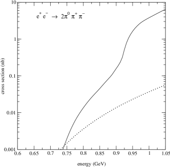
Refer to caption

Figure 8: Theoretical predictions for the cross section $\sigma(e^{+}e^{-}\to 2\pi^{0}\pi^{+}\pi^{-})$ for 0.65 $\leq E$(GeV) $\leq$ 1.05.

The analogous theoretical results for $\sigma(e^{+}e^{-}\to 2\pi^{0}\pi^{+}\pi^{-})$ are shown in Fig.Β 8. Although there are so far no data in the region below 1 GeV the theoretical cross section (full curve) connects well with the data starting at 1 GeV [17]. For this channel, the much steeper rise compared to the $2\pi^{+}2\pi^{-}$ mode is almost exclusively due to $\omega$ exchange. $a_{1}$ exchange, even though less important here, interferes constructively with $\omega$ exchange in the 1 GeV region. All other contributions are very small there.

Near the $\rho$ pole, the amplitudes are of course completely dominated by the resonant parts containing the propagator function $D_{\rho}^{-1}(q^{2})$. The cross sections at $E=M_{\rho}$ therefore determine the branching ratios for $\rho^{0}\to 4\pi$ according to the general formula

$$BR(\rho^{0}\to f)=\displaystyle\frac{M_{\rho}^{2}~{}\sigma(e^{+}e^{-}\to f)|_{E=M_{\rho}}}{12\pi~{}BR(\rho^{0}\to e^{+}e^{-})}~{}.$$ (7.1)

For the channel $2\pi^{+}2\pi^{-}$, the relevant contributions are the lowest-order amplitude with pion form factor, single $\rho$ and $a_{1}$ exchange. There is a destructive interference between the modified lowest-order amplitude on the one hand and the two single-resonance exchange amplitudes at $E=M_{\rho}$. Except for $a_{1}$ exchange, this interference is dictated by the QCD structure of $O(p^{4})$. Although the $a_{1}$ amplitude depends on our assumption (6.11) for the $a_{1}\rho\pi$ vertex the relative sign to the other two amplitudes is also fixed. The situation is a little different in the $2\pi^{0}\pi^{+}\pi^{-}$ channel because of the additional $\omega$ exchange. In this channel, the interference pattern is: lowest-order amplitude with pion form factor + $a_{1}$ exchange – single $\rho$ exchange – $\omega$ exchange. Although the couplings involved are relatively well known we assign a 40 $\%$ error to the calculated branching ratios in view of the destructive interferences:

$\displaystyle BR(\rho^{0}\to 2\pi^{+}2\pi^{-})$ $\displaystyle=$ $\displaystyle(6.7\pm 2.7)\times 10^{-6}$
$\displaystyle BR(\rho^{0}\to 2\pi^{0}\pi^{+}\pi^{-})$ $\displaystyle=$ $\displaystyle(5.0\pm 2.0)\times 10^{-6}~{}.$ (7.2)

The result for the $2\pi^{+}2\pi^{-}$ mode agrees within errors with the experimental value [24] (extracted from the cross section in Fig.Β 7 at $E=M_{\rho}$) although our mean value is almost a factor three smaller. For the $2\pi^{0}\pi^{+}\pi^{-}$ channel there is only an experimental upper limit [24] that is compatible with (7.2). There is a wide range of model predictions for the $4\pi$ decay modes of the $\rho$ as reviewed in Ref.Β [27].

We have plotted the cross sections only for energies $\stackrel{{\scriptstyle<}}{{{}_{\sim}}}$ 1 GeV because our amplitudes do not have the correct high-energy behaviour. This manifests itself already in the 1 to 2 GeV region where our cross sections exceed the experimental cross sections [17].

Scaling all four-momenta in the same way and requiring that $\sigma(e^{+}e^{-}\to 4\pi)$ decreases at least as fast as (most likely faster than) $1/E^{2}$ at large energies to satisfy the asymptotic QCD constraint, one finds that the basic current matrix element $J^{\mu}(p_{1},p_{2},p_{3},p_{4})$ in (2.6) must vanish at large energies at least as $1/E$. This criterion is not even met by the lowest-order matrix element (3.4) although it is satisfied by the modified lowest-order amplitude in (6.3) due to the pion form factor.

In addition to resummations of parts of the amplitude, additional higher-mass states must be included in order to access the region up to 2 GeV and to satisfy the high-energy constraints of QCD. The Particle Data Group lists [24] many such resonances with the appropriate quantum numbers, e.g., $\rho(1450)$, $\rho(1700)$, $f_{0}(1370)$, $f_{0}(1500)$, $f_{0}(1710)$, $\omega(1420)$, $\omega(1650)$ and states with higher spins. In the spirit of duality, all those states are expected to conspire to produce the right asymptotic behaviour of the amplitudes at high energies.

8 Conclusions

We have performed the first calculation of the processes $e^{+}e^{-}\to 4\pi$ and $\tau\to\nu_{\tau}4\pi$ with the correct structure to $O(p^{4})$ in the low-energy expansion of the standard model. In addition to the proper low-energy structure, CHPT automatically produces amplitudes with all relevant symmetries of the standard model, in our case (spontaneously and softly broken) chiral symmetry, gauge invariance, Bose symmetry and $C$ invariance.

Although the chiral amplitude to $O(p^{4})$ is only valid close to threshold it contains information how to extrapolate to the resonance region. This information on $\rho$ and scalar exchange is however not sufficient to describe the $e^{+}e^{-}$ cross sections up to energies of around 1 GeV. We have therefore included as additional contributions $\omega$, $a_{1}$ and double $\rho$ exchange that first show up at $O(p^{6})$. All necessary couplings were determined from the decay widths of the various resonances involved.

The predicted cross sections for $E\stackrel{{\scriptstyle<}}{{{}_{\sim}}}$ 1 GeV and the branching ratios $BR(\rho^{0}\to 4\pi)$ are in good agreement with available data. Our amplitudes do not have an acceptable high-energy behaviour so that additional ingredients are needed (such as higher-mass resonance exchange) to make predictions in the phenomenologically interesting region up to 2 GeV.

In the isospin limit, the $\tau$ decay amplitudes can be calculated from the annihilation amplitude for the channel $2\pi^{0}\pi^{+}\pi^{-}$ [13]. The comparison with $\tau$ decay data will be postponed until the proper high-energy behaviour has been implemented.

Acknowledgements

We thank J. PortolΓ©s for informing us of his unpublished work with A. Pich on the $a_{1}\rho\pi$ vertex and J.H. KΓΌhn for helpful informations.

A Isospin relations

From the isospin relations [13] (2.6),…,(2.9) for the four possible final states it is evident that the amplitude for the $2\pi^{0}\pi^{+}\pi^{-}$ channel is sufficient to obtain the remaining three amplitudes. From the observation that $\omega$ exchange cannot contribute to the $2\pi^{+}2\pi^{-}$, $3\pi^{0}\pi^{-}$ modes one finds immediately that none of those latter modes is sufficient to calculate the remaining ones.

The only nontrivial question333We thank Hans KΓΌhn for raising this question. concerns the channel $2\pi^{-}\pi^{+}\pi^{0}$. At first sight, one would expect that from the sum of two current matrix elements in (2.8) one cannot determine $J^{\mu}(p_{1},p_{2},p_{3},p_{4})$ itself. However, one has to take into account the symmetry relations for $J^{\mu}(p_{1},p_{2},p_{3},p_{4})$. It is the purpose of this appendix to show explicitly that knowledge of the amplitude for the $2\pi^{-}\pi^{+}\pi^{0}$ mode is also sufficient to determine all four matrix elements in the isospin limit.

For this purpose, we write the general decomposition of $J^{\mu}(p_{1},p_{2},p_{3},p_{4})$ as

$\displaystyle J^{\mu}(p_{1},p_{2},p_{3},p_{4})$ $\displaystyle=$ $\displaystyle p_{1}^{\mu}B(p_{1},p_{2},p_{3},p_{4})+p_{2}^{\mu}B(p_{2},p_{1},p_{3},p_{4})$ (A.1)
$\displaystyle+$ $\displaystyle p_{3}^{\mu}C(p_{1},p_{2},p_{3},p_{4})-p_{4}^{\mu}C(p_{1},p_{2},p_{4},p_{3})$

in terms of two invariant amplitudes that satisfy the constraints

$\displaystyle B(p_{1},p_{2},p_{3},p_{4})$ $\displaystyle=$ $\displaystyle-B(p_{1},p_{2},p_{4},p_{3})$
$\displaystyle C(p_{1},p_{2},p_{3},p_{4})$ $\displaystyle=$ $\displaystyle C(p_{2},p_{1},p_{3},p_{4})$ (A.2)

due to charge conjugation invariance and Bose symmetry. Gauge invariance leads to a further relation between $B$ and $C$ but we do not need this relation here.

The isospin relation (2.8) can now be written as

$\displaystyle\langle\pi^{-}\pi^{-}\pi^{+}\pi^{0}|V^{\mu}_{\rm cc}(0)|0\rangle/\sqrt{2}$ $\displaystyle=$ $\displaystyle p_{+}^{\mu}D(p_{+},p_{1},p_{2},p_{0})+p_{1}^{\mu}F(p_{+},p_{1},p_{2},p_{0})$ (A.3)
$\displaystyle+$ $\displaystyle p_{2}^{\mu}F(p_{+},p_{2},p_{1},p_{0})-p_{0}^{\mu}G(p_{+},p_{1},p_{2},p_{0})$

with

$\displaystyle D(p_{+},p_{1},p_{2},p_{0})$ $\displaystyle=$ $\displaystyle B(p_{+},p_{1},p_{2},p_{0})+B(p_{+},p_{2},p_{1},p_{0})$
$\displaystyle F(p_{+},p_{1},p_{2},p_{0})$ $\displaystyle=$ $\displaystyle B(p_{1},p_{+},p_{2},p_{0})+C(p_{+},p_{2},p_{1},p_{0})$ (A.4)
$\displaystyle G(p_{+},p_{1},p_{2},p_{0})$ $\displaystyle=$ $\displaystyle C(p_{+},p_{1},p_{0},p_{2})+C(p_{+},p_{2},p_{0},p_{1})~{}.$

With the symmetry relations (A.2) one easily verifies

$\displaystyle 2B(p_{1},p_{2},p_{3},p_{4})$ $\displaystyle=$ $\displaystyle D(p_{1},p_{3},p_{2},p_{4})+F(p_{2},p_{1},p_{3},p_{4})-F(p_{3},p_{1},p_{2},p_{4})$
$\displaystyle 2C(p_{1},p_{2},p_{3},p_{4})$ $\displaystyle=$ $\displaystyle-D(p_{3},p_{2},p_{1},p_{4})+F(p_{1},p_{3},p_{2},p_{4})+F(p_{2},p_{3},p_{1},p_{4})~{}.$ (A.5)

Therefore, the amplitude for the $2\pi^{0}\pi^{+}\pi^{-}$ channel can be obtained from the $2\pi^{-}\pi^{+}\pi^{0}$ amplitude. Consequently, knowledge of the $2\pi^{-}\pi^{+}\pi^{0}$ mode is enough to determine the other three amplitudes in the isospin limit.

B Vector and axial-vector mesons

Spin-1 mesons can be described either by the more conventional vector (or axial-vector) fields $V_{\mu}$ or by antisymmetric tensor fields $V_{\mu\nu}$. For matching resonance exchange amplitudes with standard CHPT amplitudes, the choice of fields is a matter of convenience. The tensor field formalism has the advantage of producing immediately the correct LECs of $O(p^{4})$ [2, 4]. On the other hand, single resonance exchange that contributes first at $O(p^{6})$ such as $\omega$ exchange is better described by vector fields [5, 28]. The two descriptions are equivalent but the transformation from one formalism to the other involves the introduction of explicit local amplitudes. Those local terms may be avoided by employing the proper formalism.

We recall first the usual normalization of a conventional massive vector field $V_{\mu}$ for a vector meson of mass $M$, with polarization vector $\varepsilon_{\mu}(p)$, and the associated propagator:

$\displaystyle\langle 0|V_{\mu}(0)|V,p\rangle$ $\displaystyle=$ $\displaystyle\varepsilon_{\mu}(p)$ (B.1)
$\displaystyle\langle 0|T\{V_{\mu}(x),V_{\nu}(0)\}|0\rangle$ $\displaystyle=$ $\displaystyle i\int\frac{d^{4}ke^{-ikx}}{(2\pi)^{4}(M^{2}-k^{2}-i\varepsilon)}\left(g_{\mu\nu}-k_{\mu}k_{\nu}/M^{2}\right)~{}.$ (B.2)

The same spin-1 particle can also be described by an antisymmetric tensor field $V_{\mu\nu}$. The corresponding one-particle matrix element and the propagator are given by [4]

$\displaystyle\langle 0|V_{\mu\nu}(0)|V,p\rangle$ $\displaystyle=$ $\displaystyle iM^{-1}\{p_{\mu}\varepsilon_{\nu}(p)-p_{\nu}\varepsilon_{\mu}(p)\}$ (B.3)
$\displaystyle\langle 0|T\{V_{\mu\nu}(x),V_{\rho\sigma}(0)\}|0\rangle$ $\displaystyle=$ $\displaystyle iM^{-2}\int\frac{d^{4}ke^{-ikx}}{(2\pi)^{4}(M^{2}-k^{2}-i\varepsilon)}\left[g_{\mu\rho}g_{\nu\sigma}(M^{2}-k^{2})\right.$ (B.4)
$\displaystyle+\left.g_{\mu\rho}k_{\nu}k_{\sigma}-g_{\mu\sigma}k_{\nu}k_{\rho}-(\mu\leftrightarrow\nu)\right]~{}.$

In many cases, the tensor field propagator can be simplified. Whenever the $\rho$ meson couples either directly to the (virtual) photon or to two pions the transverse part of (B.4) does not contribute [7] and the $\rho$ propagator may be replaced by

$\displaystyle\langle 0|T\{\rho_{\mu\nu}(x),\rho_{\rho\sigma}(0)\}|0\rangle$ $\displaystyle=$ $\displaystyle i\int\frac{d^{4}ke^{-ikx}}{(2\pi)^{4}(M^{2}-k^{2}-i\varepsilon)}\left[g_{\mu\rho}g_{\nu\sigma}-g_{\mu\sigma}g_{\nu\rho}\right]~{}.$ (B.5)

This happens to be the case for all diagrams considered involving $\rho$ exchange. The simplification does not apply for the $a_{1}$ propagator in the diagrams of Fig.Β 6.

C Numerical input

In this appendix we collect the numerical values of masses and coupling constants that we have used for the calculation of cross sections.

Chiral LECs

$F_{\pi}$ = 0.0924 GeV Β Β Β Β Β Β Β Β Β Β Β Β Β Β Β Β Β Β Β  l~1subscript~𝑙1\widetilde{l}_{1} = -2.0 $\times 10^{-3}$ Β Β Β Β Β Β Β Β Β Β Β Β Β Β Β Β Β Β Β  l~2subscript~𝑙2\widetilde{l}_{2} = 1.1 $\times 10^{-2}$
$\widetilde{l}_{3}$ = -4.6 $\times 10^{-3}$ Β Β Β Β Β Β Β Β Β Β Β Β Β Β Β Β Β Β Β  l~4subscript~𝑙4\widetilde{l}_{4} = 2.8 $\times 10^{-2}$ Β Β Β Β Β Β Β Β Β Β Β Β Β Β Β Β Β Β Β  l~6subscript~𝑙6\widetilde{l}_{6} = -1.7 $\times 10^{-2}$

Vector mesons

$M_{\rho}$ = 0.775 GeV Β Β Β Β Β Β Β Β Β Β Β Β Β Β Β Β Β Β Β  FVsubscript𝐹𝑉F_{V} = 0.14 GeV Β Β Β Β Β Β Β Β Β Β Β Β Β Β Β  GVsubscript𝐺𝑉G_{V} = 0.066 GeV
$M_{\omega}$ = 0.783 GeV Β Β Β Β Β Β Β Β Β Β Β Β Β Β Β Β Β Β Β  ΓωsubscriptΞ“πœ”\Gamma_{\omega} = 0.00844 GeV Β Β Β Β Β Β Β Β Β Β Β Β Β Β Β  gω​ρ​πsubscriptπ‘”πœ”πœŒπœ‹g_{\omega\rho\pi} = 5.7

Axial-vector meson

$M_{a_{1}}$ = 1.23 GeV Β Β Β Β Β Β Β Β Β Β Β Β Β Β Β Β Β Β Β  Ξ“a1subscriptΞ“subscriptπ‘Ž1\Gamma_{a_{1}} = 0.5 GeV
$F_{A}=F_{\pi}$ Β Β Β Β Β Β Β Β Β Β Β Β Β Β Β Β Β Β Β  c2=c3=c4subscript𝑐2subscript𝑐3subscript𝑐4c_{2}=c_{3}=c_{4} = 319

Scalar mesons

$M_{f_{0}}$ = 0.98 GeV Β Β Β Β Β Β Β Β Β Β Β Β Β Β Β Β Β Β Β  Ξ“f0subscriptΞ“subscript𝑓0\Gamma_{f_{0}} = 0.05 GeV
$M_{\sigma}$ = 0.6 GeV Β Β Β Β Β Β Β Β Β Β Β Β Β Β Β Β Β Β Β  ΓσsubscriptΞ“πœŽ\Gamma_{\sigma} = 0.6 GeV
$c_{d}$ = 0.032 GeV Β Β Β Β Β Β Β Β Β Β Β Β Β Β Β Β Β Β Β  cmsubscriptπ‘π‘šc_{m} = 0.042 GeV Β Β Β Β Β Β Β Β Β Β Β Β Β Β Β Β  c~isubscript~𝑐𝑖\widetilde{c}_{i} = $c_{i}/\sqrt{3}~{}~{}~{}(i=d,m)$

References

  • [1] S. Weinberg, Physica 96A, 327 (1979);
    H. Leutwyler, Ann. Phys. 235, 165 (1994).
  • [2] J. Gasser and H. Leutwyler, Ann. Phys. 158, 142 (1984).
  • [3] J. Gasser and H. Leutwyler, Nucl. Phys. B250, 465 (1985).
  • [4] G. Ecker, J. Gasser, A. Pich and E. de Rafael, Nucl. Phys. B321, 311 (1989).
  • [5] G. Ecker et al., Phys. Lett. B223, 425 (1989).
  • [6] F. Guerrero and A. Pich, Phys. Lett. B412, 382 (1997).
  • [7] D. GΓ³mez Dumm, A. Pich and J. PortolΓ©s, Phys. Rev. D62, 054014 (2000).
  • [8] J.A. Oller, E. Oset and J.E. Palomar, Phys. Rev. D63, 114009 (2001).
  • [9] R. Decker, P. Heiliger, H.H. Jonsson and M. Finkemeier, Z. Phys. C70, 247 (1996).
  • [10] H. Czyz and J.H. KΓΌhn, Eur. Phys. J. C18, 497 (2001).
  • [11] A.E. Bondar et al., hep-ph/0201149.
  • [12] A. Pich, in Heavy Flavours II, Eds. A.J. Buras and M. Lindner, Advanced Series on Directions in High Energy Physics 15, 453 (1998).
  • [13] J.H. KΓΌhn, Nucl. Phys. B (Proc. Suppl.) 76, 21 (1999).
  • [14] A. Pich, in Proc. 1997 Les Houches Summer School, Vol. II, p. 949, Eds. R. Gupta et al., Elsevier (Amsterdam, 1999);
    G. Ecker, Prog. Part. Nucl. Phys. 35, 1 (1995).
  • [15] R. Fischer, J. Wess and F. Wagner, Z. Phys. C3, 313 (1980).
  • [16] R.R. Akhmetshin et al. (CMD-2-Coll.), Phys. Lett. B475, 190 (2000).
  • [17] R.R. Akhmetshin et al. (CMD-2-Coll.), Phys. Lett. B466, 392 (1999).
  • [18] R. Unterdorfer, The one-loop functional of chiral $SU(2)$, hep-ph/0205162.
  • [19] G. D’Ambrosio, G. Ecker, G. Isidori and H. Neufeld, Phys. Lett. B380, 165 (1996).
  • [20] G. Colangelo, J. Gasser and H. Leutwyler, Nucl. Phys. B603, 125 (2001).
  • [21] For a recent discussion of the light scalar meson spectrum, see
    W. Ochs, hep-ph/0111309.
  • [22] M. Gell-Mann, D. Sharp and W.G. Wagner, Phys. Rev. Lett. 8, 261 (1962).
  • [23] J.J. Sakurai, Currents and Mesons, Univ. of Chicago Press (Chicago, 1969).
  • [24] Particle Data Group, Review of Particle Physics, Eur. Phys. J. C15, 1 (2000).
  • [25] A. Pich and J. PortolΓ©s, in preparation.
  • [26] J.H. KΓΌhn and A. Santamaria, Z. Phys. C48, 445 (1990).
  • [27] R.S. Plant and M.C. Birse, Phys. Lett. B365, 292 (1996).
  • [28] G. Ecker, A. Pich and E. de Rafael, Phys. Lett. B237, 481 (1990).