Abstract

We present complete solution of Altarelli-Parisi (AP) evolution equation in next-to-leading order (NLO) and obtain t-evolution of non-singlet structure function at low-x. Results are compared with HERA low-x and low-$Q^{2}$ data and also with those of complete solution in leading oder (LO) of AP evolution equation.

PACS No.: 12.38.Bx, 12.39.-x, 13.60.Hb
Keywords: Complete solution, Altarelli-Parisi equation, Structure function

1. Introduction:
The Altarelli-Parisi (AP) evolution equations [1-4] are fundamental tools to study the t(=ln$(Q^{2}/\Lambda^{2})$) and x-evolutions of structure functions, where x and $Q^{2}$ are Bjorken scaling variable and four momenta transfer in a deep inelastic scattering (DIS) process [5] respectively and $\Lambda$ is the QCD cut-off parameter. Though numerical solutions are available in the literature [6], the explorations of the possibility of obtaining analytical solutions of AP evolution equations are always interesting. In this connection, complete solutions of AP evolution equations at low-x in leading order(LO) have been obtained [7]. Its natural improvement will be the next-to-leading order (NLO) calculation.
In this paper, we present complete solution of AP evolution equation in NLO at low-x and obtain t-evolution of non-singlet structure function. Results are compared with the HERA low-x low-$Q^{2}$ data, and also with those of complete solution in LO. Here Section 1, Section 2 and Section 3 give the introduction, the necessary theory and the results and discussion respectively.

2. Theory:
The AP evolution equation for non-singlet structure function in NLO is [8]

$$\frac{\partial F_{2}^{NS}(x,t)}{\partial t}-\frac{\alpha_{s}(t)}{2\pi}\left[\frac{2}{3}\{3+4ln(1-x)\}F_{2}^{NS}(x,t)-\frac{4}{3}\int_{x}^{1}\frac{dw}{1-w}\{(1+w^{2})F_{2}^{NS}\left(\frac{x}{w},t\right)-2F_{2}^{NS}(x,t)\}\right]$$

$$-\left(\frac{\alpha_{s}(t)}{2\pi}\right)^{2}\left[(x-1)F_{2}^{NS}(x,t)\int_{0}^{1}f(w)dw+\int_{x}^{1}f(w)F_{2}^{NS}\left(\frac{x}{w},t\right)dw\right]=0$$ (1)

where,

$$f(w)=\frac{16}{9}P_{F}(w)+2P_{G}(w)+\frac{2}{3}n_{f}P_{{N}_{F}}(w)+\frac{2}{9}P_{A}(w).$$

The explicit forms of higher order kernels are [9]

$$P_{F}(w)=-\frac{2(1+w^{2})}{1-w}lnw\;ln(1-w)-\left(\frac{3}{1-w}+2w\right)lnw-\frac{1}{2}(1+w)ln^{2}w-5(1-w),$$

$$P_{G}(w)=\frac{1+w^{2}}{1-w}\left(ln^{2}w+\frac{11}{3}lnw+\frac{67}{9}-\frac{\pi^{2}}{3}\right)+2(1+w)lnw+\frac{40}{3}(1-w),$$

$$P_{{N}_{F}}(w)=\frac{2}{3}\left[\frac{1+w^{2}}{1-w}\left(-lnw-\frac{5}{3}\right)-2(1-w)\right]$$

and

$$P_{A}(w)=\frac{2(1+w^{2})}{1+w}\int_{w/(1+w)}^{1/(1+w)}\frac{dk}{k}ln\frac{1-k}{k}+2(1+w)lnw+4(1-w).$$

Running coupling constant in higher order has the form [10,11]

$$\alpha_{s}(t)=\frac{4\pi}{\beta_{o}t}\left[1-\frac{\beta_{1}lnt}{\beta_{0}^{2}t}\right]$$

for one loop with

$$\beta_{o}=\frac{33-2n_{f}}{3}\;{\rm{and}}\;\beta_{1}=\frac{306-38n_{f}}{3},$$

$n_{f}$ being the number of flavours.

Using Taylor expansion method [12] and neglecting higher order terms as discussed in our earlier works [7,13,14], $F_{2}^{NS}(x/w,t)$ can be approximated for low-x as

$$F_{2}^{NS}\left(\frac{x}{w},t\right)\simeq F_{2}^{NS}(x,t)+x\sum_{l=1}^{\infty}u^{l}\frac{\partial F_{2}^{NS}(x,t)}{\partial x}$$ (2)

where

$$x=1-w\;{\rm{and}}\;\frac{x}{1-u}=x\sum_{l=0}^{\infty}u^{l}.$$

Putting equation (2) in equation (1) and performing u-integrations we get,

$$\frac{\partial F_{2}^{NS}(x,t)}{\partial t}-\left[\frac{\alpha_{s}(t)}{2\pi}A(x)+\left(\frac{\alpha_{s}(t)}{2\pi}\right)^{2}B(x)\right]\frac{\partial F_{2}^{NS}(x,t)}{\partial x}$$

$$-\left[\frac{\alpha_{s}(t)}{2\pi}C(x)+\left(\frac{\alpha_{s}(t)}{2\pi}\right)^{2}D(x)\right]F_{2}^{NS}(x,t)=0$$ (3)

where,

$$A(x)=\frac{2}{3}\{-2xlnx+x(1-x^{2})\},$$

$$B(x)=x\int_{x}^{1}\frac{1-w}{w}f(w)dw,$$

$$C(x)=\frac{2}{3}\{3+4ln(1-x)+(x-1)(x+3)\}$$

and

$$D(x)=-\int_{0}^{x}f(w)dw+x\int_{0}^{1}f(w)dw.$$

For a possible solution, we assume that

$$\left(\frac{\alpha_{s}(t)}{2\pi}\right)^{2}=k\left(\frac{\alpha_{s}(t)}{2\pi}\right)$$

where, k is a numerical parameter to be obtained from the particular $Q^{2}$- range under study. By a suitable choice of k we can reduce the error to a minimum. Now equation (3) can be recast as

$$\frac{\partial F_{2}^{NS}(x,t)}{\partial t}-P(x,t)\frac{\partial F_{2}^{NS}(x,t)}{\partial x}-Q(x,t)F_{2}^{NS}(x,t)=0,$$ (4)

where,

$$P(x,t)=\frac{\alpha_{s}(t)}{2\pi}[A(x)+kB(x)]$$

and

$$Q(x,t)=\frac{\alpha_{s}(t)}{2\pi}[C(x)+kD(x)].$$

The general solution of equation (4) is

$$F(U,V)=0$$

where, F is an arbitrary function and

$$U(x,t,F_{2}^{NS})=C_{1}\;{\rm{and}}\;V(x,t,F_{2}^{NS})=C_{2},$$

where $C_{1}$ and $C_{2}$ are constants, form a solution of equations

$$\frac{dx}{P(x,t)}=\frac{dt}{-1}=\frac{dF_{2}^{NS}(x,t)}{-Q(x,t)}.$$ (5)

Solving equation (5) we obtain,

$$U(x,t,F_{2}^{NS})=t^{(b/t+1)}\;exp\left[\frac{b}{t}+\frac{N(x)}{a}\right]$$

and

$$V(x,t,F_{2}^{NS})=F_{2}^{NS}(x,t)\;exp[M(x)]$$

where

$$a=\frac{2}{\beta_{o}},\;b=\frac{\beta_{1}}{\beta_{o}^{2}},$$

$$N(x)=\int\frac{dx}{A(x)+kB(x)}$$

and

$$M(x)=\int\frac{C(x)+kD(x)}{A(x)+kB(x)}dx.$$

If U and V are two independent solutions of equation (4) and if $\alpha$ and$\beta$ are arbitrary constants, then

$$V=\alpha U+\beta$$

is called a complete solution of equation (4). Then the complete solution [12]

$$F_{2}^{NS}(x,t)\;exp[M(x)]=\alpha\left[t^{(b/t+1)}\;exp\left(\frac{b}{t}+\frac{N(x)}{a}\right)\right]+\beta$$

is a two-parameter family of planes. The one parameter family determined by taking $\beta=\alpha^{2}$ has equation

$$F_{2}^{NS}(x,t)\;exp[M(x)]=\alpha\left[t^{(b/t+1)}\;exp\left(\frac{b}{t}+\frac{N(x)}{a}\right)\right]+\alpha^{2}.$$ (6)

Differentiating equation (6) with respect to $\alpha$, we get

$$\alpha=-\frac{1}{2}t^{(b/t+1)}\;exp\left[\frac{b}{t}+\frac{N(x)}{a}\right].$$

Putting the value of $\alpha$ again in equation (6), we obtain

$$F_{2}^{NS}(x,t)\;exp[M(x)]=-\frac{1}{4}\left[t^{(b/t+1)}\;exp\left(\frac{b}{t}+\frac{N(x)}{a}\right)\right]^{2}.$$

Therefore,

$$F_{2}^{NS}(x,t)=-\frac{1}{4}t^{2(b/t+1)}\;exp\left[\frac{2b}{t}+\frac{2N(x)}{a}-M(x)\right].$$ (7)

Now, defining

$$F_{2}^{NS}(x,t_{o})=-\frac{1}{4}t_{o}^{2(b/t_{o}+1)}\;exp\left[\frac{2b}{t_{o}}+\frac{2N(x)}{a}-M(x)\right].$$

at $t=t_{o}$, where $t_{o}=ln(Q_{o}^{2}/\Lambda^{2})$ at any lower value $Q=Q_{o}$, we get from equation (7)

$$F_{2}^{NS}(x,t)=F_{2}^{NS}(x,t_{o})\left(\frac{t^{(b/t+1)}}{t_{o}^{(b/t_{o}+1)}}\right)^{2}\;exp\left[2b\left(\frac{1}{t}-\frac{1}{t_{o}}\right)\right]$$ (8)

which gives the t-evolution of non-singlet structure function $F_{2}^{NS}(x,t)$ in NLO. In an earlier communication [7], we suggested that for low-x in LO

$$F_{2}^{NS}(x,t)=F_{2}^{NS}(x,t_{o})\left(\frac{t}{t_{o}}\right)^{2}.$$ (9)

We observe that if b tends to zero, then equation (8) tends to equation(9), i.e., solution of NLO equation goes to that of LO equation. Physically b tends to zero means number of flavours is high.
Again defining,

$$F_{2}^{NS}(x_{o},t)=-\frac{1}{4}t^{(b/t+1)}\;exp\left[\frac{2b}{t}+\frac{2N(x)}{a}-M(x)\right]_{x=x_{o}},$$

we obtain from equation (7)

$$F_{2}^{NS}(x,t)=F_{2}^{NS}(x_{o},t)\;exp\int_{x_{o}}^{x}\left[\frac{2}{a}.\frac{1}{A(x)+kB(x)}-\frac{C(x)+kD(x)}{A(x)+kB(x)}\right]dx$$ (10)

which gives the x-evolution of non-singlet structure function $F_{2}^{NS}(x,t)$ in NLO.
Proton and neutron structure functions measured in deep inelastic electro-production can be written in terms of singlet and non-singlet quark distribution functions as

$$F_{2}^{p}(x,t)=\frac{5}{18}F_{2}^{S}(x,t)+\frac{3}{18}F_{2}^{NS}(x,t)$$

and

$$F_{2}^{n}(x,t)=\frac{5}{18}F_{2}^{S}(x,t)-\frac{3}{18}F_{2}^{NS}(x,t).$$

These equations give

$$F_{2}^{NS}=3(F_{2}^{p}-F_{2}^{n})$$

from which we can calculate experimental values of $F_{2}^{NS}$ in t and x ranges given in $F_{2}^{p}$ and $F_{2}^{n}$.

3. Results and Discussion:
In the present paper, we compare our results of t-evolution of non-singlet structure functions from equation (8) with the HERA low-x and low-$Q^{2}$ data [15]. Here proton and neutron structure functions are measured in the range $2\leq Q^{2}\leq 50\;GeV^{2}$. Moreover here $P_{T}\leq 200\;MeV$, where $P_{T}$ is the transverse momentum of the final state baryon. We consider number of flavours $n_{f}$=4.

In figures 1(a-c) we present our results of t-evolution of non-singlet structure functions $F_{2}^{NS}$ (solid lines) for the representative values of x given to test the evolution equation (8) in next-to-leading order. Agreement is found to be good. In the same figures we also plot the results of t-evolutions of non-singlet structure functions $F_{2}^{NS}$ (dashed lines) for the complete solutions from equation (9) in leading order. Data points at lowest-$Q^{2}$ values in the figures are taken as inputs. We observe that t-evolutions are slightly steeper in NLO calculations then those of LO. We can also calculate x-evolution of non-singlet structure functions at low-x from equation (10). But it involves complicated triple integrations and we keep it as our subsequent work.

In figure 2 we plot ${T(t)}^{2}$ and kT(t) against $Q^{2}$ in the $Q^{2}$ range $2\leq Q^{2}\leq 50\;GeV^{2}$ as required by our data used[15]. Though the explicit value of k is not necessary in calculating t-evolution of $F_{2}^{NS}$, yet we observe that for k= 0.027, errors become minimum and varies from 17.68% to -13.68% in the $Q^{2}$ range $2\leq Q^{2}\leq 50\;GeV^{2}$.

Acknowledgement:
We are grateful to G. A. Ahmed of Department of Physics and N. Basumatary of Department of Information Technology of Tezpur University for the help in the computational part of this work. One of us (JKS) is grateful to UGC, New Delhi for the financial assistance to this work in the form of a major research project.

References:
$[1]$G. Altarelli and G. Parisi, Nucl. Phys. B 126 (1977) 298.
$[2]$G. Altarelli, Phy. Rep. 81 (1981) 1.
$[3]$V.N. Gribov and L.N. Lipatov, Sov. J. Nucl. Phys. 20 (1975) 94.
$[4]$Y.L. Dokshitzer, Sov. Phy. JETP 46 (1977) 641.
$[5]$F. Halzen and A. D. Martin, Quarks and Leptons: An Introductory Course in Modern Particle Physics, John and Wiley (1984).
$[6]$M. Miyama and S. Kumano, hep-ph/9508246 (1995).
$[7]$R. Rajkhowa and J.K. Sarma, hep-ph/0202263 (2002).
$[8]$A. Deshamukhya and D.K. Choudhury, Proc. 2nd Regional Conf. Phys. Research in North-East, Guwahati, India, October, 2001 (2001) 34.
$[9]$G.Curci, W.Furmanski and R.Petronzio, Nucl. Phys. B175 (1980) 27.
$[10]$L.F. Abbott and R.M. Barnett, Ann.Phys. 125 (1980) 276.
$[11]$A. Saikia and D.K. Choudhury, Pramana-J. Phys. 38 (1992) 313.
$[12]$F. Ayres Jr., Differential Equations, Schaum’s Outline Series, McGraw-Hill (1952).
$[13]$J.K. Sarma and B. Das, Phy. Lett. B304 (1993) 323.
$[14]$J.K. Sarma, D.K. Choudhury and G.K. Medhi, Phys. Lett. B403 (1997) 139.
$[15]$M. Arneodo et al., hep/961031, NMC, Nucl. Phy. B483 (1997).

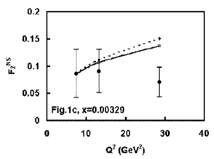
Figure 1: t-evolutions of non-singlet structure functions $F_{2}^{NS}(x,t)$(solid lines) for the representative values of x given in the figures. Data points at lowest-$Q^{2}$ values in the figures are taken as input to test NLO t-evoluation of non-singlet structure functions $F_{2}^{NS}$ from equation (8). In the same figures we also plot the results of t-evolutions of non-singlet structure functions $F_{2}^{NS}$ (dashed lines) for LO from equation (9).

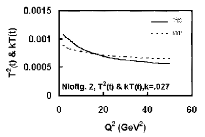
Figure 2: ${T(t)}^{2}$ and kT(t) against $Q^{2}$ in the range $2\leq Q^{2}\leq 50\;GeV^{2}$ for k=0.027.

References:

[1]delimited-[]1[1]