Resonant and Non–Resonant Effects in Photon–Technipion Production at Lepton Colliders

Lepton collider experiments can search for light technipions in final states made striking by the presence of an energetic photon: ${\mathrm{{e^{+}}}\mathrm{{e^{-}}}}\to\mathrm{{\gamma}}\mathrm{{\Pi_{T}}}$. To date, searches have focused on either production through anomalous coupling of the technipions to electroweak gauge bosons or on production through a technivector meson ($\mathrm{{\rho_{T}}}$, $\mathrm{{\omega_{T}}}$) resonance. This paper creates a combined framework in which both contributions are included. This will allow stronger and more accurate limits on technipion production to be set using existing data from LEP or future data from a higher-energy linear collider. We provide explicit formulas and sample calculations (analytic and Pythia) in the framework of the Technicolor Straw Man Model, a model that includes light technihadrons.

1 Introduction

Modern technicolor [1] models require a walking gauge coupling [2, 3] to avoid large flavor–changing neutral currents and extra top quark dynamics such as topcolor interactions [4] to generate the large top quark mass. To incorporate these innovations, a large number of technifermion doublets, $N_{D}$, must typically be present in the model to perform such crucial tasks as flattening the beta function and breaking the topcolor interactions to ordinary color [5, 6, 7, 8]. This large number of doublets also suppresses the technihadron mass scale, resulting in a small technipion decay constant

$$F_{\mathrm{T}}\approx\frac{246\,\mathrm{GeV}}{\sqrt{N_{D}}}\ ,$$ (1.1)

and very light technipions [5]. For example, if $N_{D}=10$, $F_{\mathrm{T}}\approx 80\,\mathrm{GeV}$. With such a low mass scale, the question of collider phenomenology becomes of immediate interest, since the lowest lying technimeson states could be produced directly at current or near future experiments [9, 10].

This study discusses production of light technimeson states at lepton colliders. We focus on providing a complete phenomenological description of both resonant and non-resonant technimeson production. The framework created here should enable the LEP experiments to obtain more comprehensive limits on light technihadrons from their final analyses than have been extracted thus far with the more limited methods available previously [10, 11]. We perform several sample calculations for colliders with $\sqrt{s}$ of up to a few hundred GeV, consistent with our interest in the LEP data. However, our methods are also applicable to future linear colliders at higher energies.

We use the Technicolor Straw Man Model (TCSM) [12, 13] as a benchmark for assessing the experimental visibility of technipion production. The TCSM assumes that techni–isospin is a good symmetry, and that, in analogy with QCD, the lightest technimesons are constructed solely from the lightest technifermion weak doublet, $(\mathrm{{T_{U}}},\mathrm{{T_{D}}})$, which transform as ${\mathrm{SU}({3})}_{C}$ singlets and ${\mathrm{SU}({N_{\mathrm{TC}}})}$ fundamentals. The members of the doublet are assigned electric charges $Q_{\mathrm{{U}}}$ and $Q_{\mathrm{{D}}}$ respectively. This flavor and gauge structure gives rise to the same type of spectrum as two–flavor QCD: namely, an isotriplet and isosinglet of pseudoscalar, pseudo-goldstone modes, the $\mathrm{{\mathrm{{\pi}}_{T}}}^{0,\pm}$ and $\mathrm{{\mathrm{{\pi}}_{T}^{\prime}}}^{0}$, and an isotriplet and isosinglet of vector modes, the $\mathrm{{\rho_{T}}}^{0,\pm}$ and $\mathrm{{\omega_{T}}}^{0}$. The electric charge assignments of the mesons require that $Q_{\mathrm{{U}}}-Q_{\mathrm{{D}}}=1$. Since we assume that techni–isospin symmetry is a good symmetry, the technipions should be nearly degenerate in mass, as should the technivector modes. When both the $\mathrm{{\mathrm{{\pi}}_{T}}}$ and $\mathrm{{\mathrm{{\pi}}_{T}^{\prime}}}$ are possible final states for a given process, we will refer to both collectively by the notation $\mathrm{{\Pi_{T}}}$.

Calculation of matrix elements involving the technihadron bound states at energies below the technicolor scale, $\Lambda_{\mathrm{TC}}$, in the full non-abelian technicolor model requires use of low energy phenomenological models. In the recent past, two different types of descriptions have been widely used for fermion–antifermion annihilation to a technipion plus electroweak gauge boson. In these the initial–state fermions couple with standard weak couplings to the appropriate electroweak gauge bosons in the $s$–channel. The descriptions differ in how they handle the weak gauge boson transition to the final state, and can be divided into

1. Anomaly–Mediated Approach: the gauge boson couples to the $\mathrm{{\Pi_{T}}}$ in the final state through a technifermion ($\mathrm{{f_{T}}}$) triangle anomaly [14, 15] (Figure 1a), and

2. Technivector ($\mathrm{{V_{T}}}$) Dominated Approach: the gauge boson undergoes a kinetic mixing (that is, a term proportional to $s$ in the inverse propagator matrix) into a $\mathrm{{\rho_{T}}}$ or $\mathrm{{\omega_{T}}}$, which then decays directly into the $\mathrm{{\Pi_{T}}}$ in the final state [6, 12, 13] (Figure 1b).

Both schemes have direct analogues in Standard Model QCD calculations. Our goal is to synthesize these approaches within the TCSM to eliminate the shortcomings of each.

In Section 2, we review the details of both the anomaly–mediated and $\mathrm{{V_{T}}}$–dominated approaches to the TCSM and indicate the limitations of their individual descriptions of technimeson production at lepton colliders. Our calculations focus on the process ${\mathrm{{e^{+}}}\mathrm{{e^{-}}}}\to\mathrm{{\gamma}}\mathrm{{\Pi_{T}}}$ because kinematic and phase space considerations should give it a larger cross–section than processes involving final–state weak bosons. In Section 2.3 we discuss how to combine the strengths of both approaches within the TCSM framework. In Section 3 we compare analytic cross section predictions for ${\mathrm{{e^{+}}}\mathrm{{e^{-}}}}\to\mathrm{{\gamma}}\mathrm{{\Pi_{T}}}$ in all three approaches. In Section 3.2 we discuss the predictions for the mass recoiling against the photon in the process ${\mathrm{{e^{+}}}\mathrm{{e^{-}}}}\to\mathrm{{\gamma}}\mathrm{{\Pi_{T}}}$ within the combined framework as implemented in Pythia.

2 Phenomenological Approaches

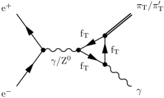
1a Anomaly model

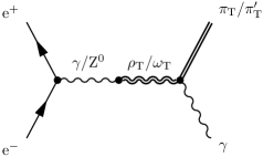
1b $\mathrm{{V_{T}}}$-dominance model

Figure 1: 1a The anomaly–mediated production mechanism of a $\mathrm{{\gamma}}\mathrm{{\Pi_{T}}}$ final state. 1b The $\mathrm{{V_{T}}}$–dominated production mechanism to lowest order in $\alpha$.

2.1 Anomaly Mediation

In the anomaly–mediated schemes, we assume that the lowest lying observable states, the $\mathrm{{\mathrm{{\pi}}_{T}}}$ and $\mathrm{{\mathrm{{\pi}}_{T}^{\prime}}}$, are pseudo–Nambu–Goldstone modes of the $\mathrm{SU}({N_{\mathrm{TC}}})$ technicolor theory, in direct analogy to the QCD pion. The coupling of these $\mathrm{{\Pi_{T}}}$ goldstone modes to a pair, $G_{1}$ and $G_{2}$, of electroweak gauge bosons is given by [16, 2]

$$\mathcal{M}(G_{1}(q)\to G_{2}(p_{1})\mathrm{{\Pi_{T}}}(p_{2}))=N_{\mathrm{TC}}\mathcal{V}_{G_{1}G_{2}\mathrm{{\Pi_{T}}}}\frac{g_{1}g_{2}}{8\pi^{2}F_{\mathrm{T}}}\varepsilon^{\mu\nu\lambda\rho}\epsilon_{\mu}(q)\epsilon^{*}_{\nu}(p_{1})q_{\lambda}p_{1\rho}$$ (2.1)

where $N_{\mathrm{TC}}$ is the number of technicolors, the $g_{i}$ are the couplings of the gauge groups, $q$ and $p_{1}$ are the momenta and the $\epsilon_{i}$ the polarizations of the gauge bosons. The triangle anomaly factor, $\mathcal{V}_{G_{1}G_{2}\mathrm{{\Pi_{T}}}}$, is given by [16, 2]

$$\mathcal{V}_{G_{1}G_{2}\mathrm{{\Pi_{T}}}}=\operatorname{Tr}\left[T^{a}\left(\left\{T_{1},T_{2}\right\}_{L}+\left\{T_{1},T_{2}\right\}_{R}\right)\right]\ .$$ (2.2)

Here $T_{i}$ is the generator associated with the gauge boson $G_{i}$, and $T^{a}$ is the generator of the axial current associated with the technipion

$$j^{\mu a}_{5}=\overline{\psi}\gamma^{{\mu}}\gamma_{5}T^{a}\psi\ ;$$ (2.3)

in this convention, the generators are normalized such that $\operatorname{Tr}{\left(T^{a}T^{b}\right)}=\frac{1}{2}\delta^{ab}$ .

Using these expressions, we can calculate the cross section for ${\mathrm{{e^{+}}}\mathrm{{e^{-}}}}\to\mathrm{{\gamma}}\mathrm{{\Pi_{T}}}$ in an anomaly mediated framework, obtaining [15]

$${\mathrm{\sigma}({{\mathrm{{e^{+}}}\mathrm{{e^{-}}}}\to\mathrm{{\gamma}}\mathrm{{\Pi_{T}}}})}=\frac{\alpha_{\mathrm{em}}^{3}N_{\mathrm{TC}}^{2}}{192\pi^{2}F_{\mathrm{T}}^{2}}\left(s-M_{\mathrm{{\Pi_{T}}}}^{2}\right)^{3/2}\\ \times\left[\left|\left(\mathcal{V}_{\mathrm{{\gamma}}\mathrm{{\gamma}}\mathrm{{\Pi_{T}}}}\Delta_{\mathrm{{\gamma}}\mathrm{{\gamma}}}(s)-\frac{2\zeta_{\mathrm{{e}}L}\mathcal{V}_{\mathrm{{\gamma}}\mathrm{{Z^{0}}}\mathrm{{\Pi_{T}}}}}{\sin 2\theta_{W}}\Delta_{\mathrm{{Z^{0}}}\mathrm{{Z^{0}}}}(s)\right)\right|^{2}+\left|\left(\mathcal{V}_{\mathrm{{\gamma}}\mathrm{{\gamma}}\mathrm{{\Pi_{T}}}}\Delta_{\mathrm{{\gamma}}\mathrm{{\gamma}}}(s)-\frac{2\zeta_{\mathrm{{e}}R}\mathcal{V}_{\mathrm{{\gamma}}\mathrm{{Z^{0}}}\mathrm{{\Pi_{T}}}}}{\sin 2\theta_{W}}\Delta_{\mathrm{{Z^{0}}}\mathrm{{Z^{0}}}}(s)\right)\right|^{2}\right]\ ,$$ (2.4)

where $\Delta_{\mathrm{{\gamma}}\mathrm{{\gamma}}}(s)^{-1}=s$, $\Delta_{\mathrm{{Z^{0}}}\mathrm{{Z^{0}}}}(s)^{-1}=s-M_{\mathrm{{Z^{0}}}}^{2}+i\Gamma_{\mathrm{{Z^{0}}}}M_{\mathrm{{Z^{0}}}}$, and $\zeta_{\mathrm{{e}}\lambda}=T^{3}_{\mathrm{{e}}_{\lambda}}+\sin^{2}\theta_{W}$ for chiralities $\lambda=L,R$. For the TCSM, the anomaly factors involving the $\mathrm{{\mathrm{{\pi}}_{T}}}$ and $\mathrm{{\mathrm{{\pi}}_{T}^{\prime}}}$ are given by [11, 12]

$$\mathcal{V}_{\mathrm{{\gamma}}\mathrm{{\gamma}}\mathrm{{\mathrm{{\pi}}_{T}}}} =2\left(Q_{\mathrm{{U}}}+Q_{\mathrm{{D}}}\right)c_{\chi} \mathcal{V}_{\mathrm{{\gamma}}\mathrm{{Z^{0}}}\mathrm{{\mathrm{{\pi}}_{T}}}} =\frac{\left(Q_{\mathrm{{U}}}+Q_{\mathrm{{D}}}\right)\left(1-4\sin^{2}\theta_{W}\right)c_{\chi}}{\sin 2\theta_{W}}$$ (2.5)

$$\mathcal{V}_{\mathrm{{\gamma}}\mathrm{{\gamma}}\mathrm{{\mathrm{{\pi}}_{T}^{\prime}}}} =2\left(Q_{\mathrm{{U}}}^{2}+Q_{\mathrm{{D}}}^{2}\right)c_{\chi^{\prime}} \mathcal{V}_{\mathrm{{\gamma}}\mathrm{{Z^{0}}}\mathrm{{\mathrm{{\pi}}_{T}^{\prime}}}} =\frac{\left(1-4\sin^{2}\theta_{W}\left(Q_{\mathrm{{U}}}^{2}+Q_{\mathrm{{D}}}^{2}\right)\right)c_{\chi^{\prime}}}{\sin 2\theta_{W}}\ .$$ (2.6)

A more detailed discussion of this and other processes in the anomaly framework can be found in [15, 17, 11]. Using this framework, limits on various TC models have been extracted from published LEP data on final states with photons, large missing energy, jet pairs, or $b\bar{b}$ pairs in [11]. Production of technipions in the anomaly framework at future $\mathrm{{e^{+}}}$$\mathrm{{e^{-}}}$ colliders has been discussed in [18]

The anomaly mediated description has the dual strengths of conceptual clarity and relative ease of calculation. It does, however, have a flaw which would not be present in a complete technicolor model and and which prevents it from being an appropriate description in all kinematic regimes. Since this scheme does not take into account the heavier technimeson bound states of the technifermions (the states equivalent to the QCD $\rho$ and $\omega$, among others), it can only provide a valid description of technicolor physics in kinematic regions well below the propagator poles of the lightest technivector meson [12].

2.2 Technivector Meson Dominance in the TCSM

To describe the kinematic regime near the technivector poles, an alternative phenomenological approach is needed; typically this takes the form of the $\mathrm{{V_{T}}}$–dominance scheme introduced above. For the TCSM, a framework has been developed by Lane [12, 13]. Conceptually, the collider experiments generate electroweak gauge bosons via the direct couplings of standard model particles to the electroweak gauge fields. The electroweak gauge bosons then convert into technivector mesons through mixing terms in the vector propagator matrix (for illustration, we display the inverse of the neutral propagator matrix here)

$$\Delta_{0}^{-1}(s)=\left(\begin{array}[]{cccc}s&0&sf_{\mathrm{{\gamma}}\mathrm{{\rho_{T}}}}&sf_{\mathrm{{\gamma}}\mathrm{{\omega_{T}}}}\\ 0&s-\mathcal{M}_{\mathrm{{Z^{0}}}}^{2}&sf_{\mathrm{{Z^{0}}}\mathrm{{\rho_{T}}}}&sf_{\mathrm{{Z^{0}}}\mathrm{{\omega_{T}}}}\\ sf_{\mathrm{{\gamma}}\mathrm{{\rho_{T}}}}&sf_{\mathrm{{Z^{0}}}\mathrm{{\rho_{T}}}}&s-\mathcal{M}_{\mathrm{{\rho_{T}}}}^{2}&0\\ sf_{\mathrm{{\gamma}}\mathrm{{\omega_{T}}}}&sf_{\mathrm{{Z^{0}}}\mathrm{{\omega_{T}}}}&0&s-\mathcal{M}_{\mathrm{{\omega_{T}}}}^{2}\end{array}\right)\begin{array}[]{c}\\ \\ \\ \ ,\end{array}$$ (2.7)

where the masses, $\mathcal{M}_{V}=M_{V}^{2}-i\sqrt{s}\Gamma_{V}$ include $s$–dependent width effects. The mixing factors are $f_{\mathrm{{\gamma}}\mathrm{{\rho_{T}}}}=\xi$, $f_{\mathrm{{\gamma}}\mathrm{{\omega_{T}}}}=\xi(Q_{\mathrm{{U}}}+Q_{\mathrm{{D}}})$, $f_{\mathrm{{Z^{0}}}\mathrm{{\rho_{T}}}}=\xi\cot 2\theta_{W}$, and $f_{\mathrm{{Z^{0}}}\mathrm{{\omega_{T}}}}=-\xi(Q_{\mathrm{{U}}}+Q_{\mathrm{{D}}})\tan\theta_{W}$ where $\xi^{2}=\alpha_{em}/\alpha_{\mathrm{{\rho_{T}}}}$ [12, 13]. These vector technimesons decay into the lighter spinless technimesons, electroweak bosons, and fermion–antifermion pairs.

The TCSM was developed to describe technihadron production at high–energy hadron colliders for which the convoluted parton distributions sweep over the $\mathrm{{\rho_{T}}}/\mathrm{{\omega_{T}}}$ resonance poles. In its original form, it did not properly include contributions that are far below the poles [12]. However, at an $\mathrm{{e^{+}}}$$\mathrm{{e^{-}}}$ collider such as LEP (or a future linear collider), the machine’s operating energy $\sqrt{s}$ may be well away from the resonance. For those cases, it is necessary to include off–resonance contributions. At the very least, this may allow more stringent limits on technihadron masses and couplings to be derived from searches in ${\mathrm{{e^{+}}}\mathrm{{e^{-}}}}$ colliders.

The coupling of the initial state electrons to the gauge boson is unchanged from the Standard Model. The couplings of the technivectors, $\mathrm{{\rho_{T}}}$ and $\mathrm{{\omega_{T}}}$, to the final state technipion and photon are given by the TCSM matrix element [12]

$$\begin{split}\mathcal{M}\left(V_{T}(q)\to\mathrm{{\gamma}}(p_{1})\mathrm{{\Pi_{T}}}(p_{2})\right)=&\frac{eV_{V_{T}\mathrm{{\gamma}}\mathrm{{\Pi_{T}}}}}{M_{V}}\varepsilon^{\mu\nu\lambda\rho}\epsilon_{\mu}(q)\epsilon^{*}_{\nu}(p_{1})q_{\lambda}p_{1\rho}+\\ &\frac{eA_{V_{T}\mathrm{{\gamma}}\mathrm{{\Pi_{T}}}}}{M_{A}}\left(\epsilon(q)\cdot\epsilon^{*}(p_{1})q\cdot p_{1}-\epsilon(q)\cdot p_{1}\epsilon^{*}(p_{1})\cdot q\right)\ ,\end{split}$$ (2.8)

where the first (second) term is the vector (axial) contribution, and $M_{V}$ and $M_{A}$ are dynamical mass parameters of the same order that set the strengths of these terms (for simplicity we set them equal below). The relevant axial couplings ($A_{V_{T}\mathrm{{\gamma}}\mathrm{{\Pi_{T}}}}$) are zero; the relevant vector ($V_{V_{T}\mathrm{{\gamma}}\mathrm{{\Pi_{T}}}}$) couplings are [12]

$$V_{\mathrm{{\rho_{T}}}\mathrm{{\gamma}}\mathrm{{\mathrm{{\pi}}_{T}}}} =2\left(Q_{\mathrm{{U}}}+Q_{\mathrm{{D}}}\right)c_{\chi} V_{\mathrm{{\rho_{T}}}\mathrm{{\gamma}}\mathrm{{\mathrm{{\pi}}_{T}^{\prime}}}} =c_{\chi^{\prime}}$$ (2.9)

$$V_{\mathrm{{\omega_{T}}}\mathrm{{\gamma}}\mathrm{{\mathrm{{\pi}}_{T}}}} =c_{\chi} V_{\mathrm{{\omega_{T}}}\mathrm{{\gamma}}\mathrm{{\mathrm{{\pi}}_{T}^{\prime}}}} =2\left(Q_{\mathrm{{U}}}+Q_{\mathrm{{D}}}\right)c_{\chi^{\prime}}.$$ (2.10)

A list of analogous couplings for other gauge bosons and $\mathrm{{V_{T}}}$ in the TCSM is given in [12].

The cross section for ${\mathrm{{e^{+}}}\mathrm{{e^{-}}}}\to\mathrm{{\gamma}}\mathrm{{\Pi_{T}}}$ is given by [12]

$${\mathrm{\sigma}({{\mathrm{{e^{+}}}\mathrm{{e^{-}}}}\to\mathrm{{\gamma}}\mathrm{{\Pi_{T}}}})}=\frac{\pi\alpha_{\mathrm{em}}^{2}}{108M_{V}^{2}}\frac{\left(s-M_{\mathrm{{\Pi_{T}}}}^{2}\right)^{4}}{s^{2}}\left[\left|\mathcal{G}_{\mathrm{{e}}L}^{V\mathrm{{\gamma}}\mathrm{{\Pi_{T}}}}\right|^{2}+\left|\mathcal{G}_{\mathrm{{e}}R}^{V\mathrm{{\gamma}}\mathrm{{\Pi_{T}}}}\right|^{2}+\left|\mathcal{G}_{\mathrm{{e}}L}^{A\mathrm{{\gamma}}\mathrm{{\Pi_{T}}}}\right|^{2}+\left|\mathcal{G}_{\mathrm{{e}}R}^{A\mathrm{{\gamma}}\mathrm{{\Pi_{T}}}}\right|^{2}\right]\ .$$ (2.11)

The $\mathcal{G}_{\mathrm{{e}}\lambda}^{X\mathrm{{\gamma}}\mathrm{{\Pi_{T}}}}$ are given by

$$\mathcal{G}_{\mathrm{{e}}\lambda}^{X\mathrm{{\gamma}}\mathrm{{\Pi_{T}}}}=\sum_{V_{T}=\mathrm{{\rho_{T}}},\mathrm{{\omega_{T}}}}X_{V_{T}\mathrm{{\gamma}}\mathrm{{\Pi_{T}}}}\mathcal{F}_{\mathrm{{e}}\lambda}^{V_{T}}(s)\ ,$$ (2.12)

where the $X_{V_{T}\mathrm{{\gamma}}\mathrm{{\Pi_{T}}}}$ are the vector and axial couplings of the vector technimesons to the technipion and photon, and

$$\mathcal{F}_{\mathrm{{e}}\lambda}^{V_{T}}(s)=e\Delta_{\mathrm{{\gamma}}V_{T}}(s)+\frac{2\zeta_{\mathrm{{e}}\lambda}}{\sin 2\theta_{W}}\Delta_{\mathrm{{Z^{0}}}V_{T}}(s)$$ (2.13)

includes the coupling of the initial state electrons to the gauge bosons and the propagator elements that mix the vector bosons with the technivector mesons. A more detailed discussion of this and other processes in the $\mathrm{{V_{T}}}$–dominance approach to the TCSM can be found in [12, 13]. The DELPHI and OPAL experiments at LEP [10] used $\mathrm{{V_{T}}}$–dominance to obtain limits on ${\mathrm{{e^{+}}}\mathrm{{e^{-}}}}\to\mathrm{{\rho_{T}}},\mathrm{{\omega_{T}}}\to\mathrm{{\gamma}}\mathrm{{\Pi_{T}}}$ and related processes in the TCSM.

2.3 Combining Both Schemes

The center of mass energies of LEP and proposed future linear colliders are comparable to the expected masses of the lightest technihadrons in low–scale technicolor: a few hundred GeV. Hadron collider experiments are sensitive only to resonant technivector contributions, and therefore need consider only contributions from the poles. In contrast, lepton collider experiments have a broader sensitivity and may well be operating off the poles — especially when their location is unknown. For an $\mathrm{{e^{+}}}$$\mathrm{{e^{-}}}$ collider operating slightly below the poles, it is especially important to understand how the resonant and non–resonant contributions are combined.

Schematically, we would like to define a matrix element that interpolates between the anomaly mediated matrix element at the $\mathrm{{\Pi_{T}}}$ production threshold and the $\mathrm{{V_{T}}}$-dominated matrix element in the region of the technivector poles, that is

$$\mathcal{M}_{\text{combined}}=\mathcal{M}_{\text{anomaly}}\left[f(s)\right]^{n}+\mathcal{M}_{\mathrm{{V_{T}}}}\left[1-f(s)\right]^{n}\ ,$$

where the interpolating function $f(s)$ has the limits $f(s\to 0)\to 1$ and $f(s\to M_{\mathrm{{\rho_{T}}},\mathrm{{\omega_{T}}}})\to 0$. Numerically, we find that either the anomaly–mediated or the $\mathrm{{V_{T}}}$–mediated matrix element completely dominates the cross section, except in a relatively narrow region approximately midway between threshold and the first technivector pole, where they are of approximately equal magnitude (see Figure 2). Because of this behavior, we gain little by implementing such a complicated scheme rather than simply taking $n\to 0$ in the above interpolation, that is, simply adding the relevant matrix elements everywhere. This gives us the correct limits, up to numerically irrelevant errors.

Adding the matrix elements has several virtues: it reproduces the correct cross-section both well below and in the region of the technivector meson resonances, and it is simple to implement. In addition, as will be shown shortly, the combined cross-sections still respect unitarity bounds in the energy range of experimental interest. At much higher energies, our description will break down because additional resonances and continuum technifermion production will emerge, but that is not relevant to our purposes.

Since the matrix element in Equation 2.1 for the anomaly–mediated coupling and the vectorial component in Equation 2.8 of the matrix element in the $\mathrm{{V_{T}}}$-dominated scheme have the same Lorentz structure, we add them. From the combined matrix elements, we obtain the cross section for ${\mathrm{{e^{+}}}\mathrm{{e^{-}}}}\to G\mathrm{{\Pi_{T}}}$, where $G$ is a photon or a transversely polarized $\mathrm{{Z^{0}}}$:

$${\mathrm{\sigma}({{\mathrm{{e^{+}}}\mathrm{{e^{-}}}}\to G\mathrm{{\Pi_{T}}}})}=\\ \frac{\pi\alpha_{\mathrm{em}}^{2}}{12s}\lambda({s},{M_{G}^{2}},{M_{\mathrm{{\Pi_{T}}}}^{2}})^{3/2}\left(\left|\mathcal{G}_{\mathrm{{e}}L}^{VG\mathrm{{\Pi_{T}}}}(s)\right|^{2}+\left|\mathcal{G}_{\mathrm{{e}}R}^{VG\mathrm{{\Pi_{T}}}}(s)\right|^{2}+\left|\mathcal{G}_{\mathrm{{e}}L}^{AG\mathrm{{\Pi_{T}}}}(s)\right|^{2}+\left|\mathcal{G}_{\mathrm{{e}}R}^{AG\mathrm{{\Pi_{T}}}}(s)\right|^{2}\right)\\ +\frac{\pi\alpha_{\mathrm{em}}^{2}M_{G}^{2}}{2}\lambda({s},{M_{G}^{2}},{M_{\mathrm{{\Pi_{T}}}}^{2}})^{1/2}\left(\left|\mathcal{G}_{\mathrm{{e}}L}^{AG\mathrm{{\Pi_{T}}}}(s)\right|^{2}+\left|\mathcal{G}_{\mathrm{{e}}R}^{AG\mathrm{{\Pi_{T}}}}(s)\right|^{2}\right)\ .$$ (2.14)

Here $\lambda({a},{b},{c})=a^{2}+b^{2}+c^{2}-2ab-2ac-2bc$ and $M_{G}$ is the mass of the final state gauge boson. The vectorial couplings for a given fermion helicity $\lambda$, including both $\mathrm{{V_{T}}}$ and anomaly terms, is given by

$$\mathcal{G}_{\mathrm{{e}}\lambda}^{VG\mathrm{{\Pi_{T}}}}(s)=\sum_{V_{T}=\mathrm{{\rho_{T}}},\mathrm{{\omega_{T}}}}\frac{V_{V_{T}G\mathrm{{\Pi_{T}}}}}{M_{V}}\left(Q_{\mathrm{{e}}}\Delta_{\mathrm{{\gamma}}V_{T}}(s)+\frac{2\zeta_{\mathrm{{e}}\lambda}}{\sin 2\theta_{W}}\Delta_{\mathrm{{Z^{0}}}V_{T}}(s)\right)\\ +\frac{eN_{\mathrm{TC}}}{8\pi^{2}F_{\mathrm{T}}}\sum_{G^{\prime}=\mathrm{{\gamma}},\mathrm{{Z^{0}}}}\mathcal{V}_{G^{\prime}G\mathrm{{\Pi_{T}}}}\left(Q_{\mathrm{{e}}}\Delta_{\mathrm{{\gamma}}G^{\prime}}(s)+\frac{2\zeta_{\mathrm{{e}}\lambda}}{\sin 2\theta_{W}}\Delta_{\mathrm{{Z^{0}}}G^{\prime}}(s)\right)\ ,$$ (2.15)

where in contrast to Equation 2.4, the anomaly contribution now includes off–diagonal mixing terms in the propagator, $\Delta_{\mathrm{{Z^{0}}}\mathrm{{\gamma}}}(s)$ and $\Delta_{\mathrm{{\gamma}}\mathrm{{Z^{0}}}}(s)$, that are induced by the presence of the $\mathrm{{\rho_{T}}}$ and $\mathrm{{\omega_{T}}}$ in the vector spectrum. The axial couplings are given by

$$\mathcal{G}_{\mathrm{{e}}\lambda}^{AG\mathrm{{\Pi_{T}}}}(s)=\sum_{V_{T}=\mathrm{{\rho_{T}}},\mathrm{{\omega_{T}}}}\frac{A_{V_{T}G\mathrm{{\Pi_{T}}}}}{M_{V}}\left(Q_{\mathrm{{e}}}\Delta_{\mathrm{{\gamma}}V_{T}}(s)+\frac{2\zeta_{\mathrm{{e}}\lambda}}{\sin 2\theta_{W}}\Delta_{\mathrm{{Z^{0}}}V_{T}}(s)\right)\ .$$ (2.16)

Once again, the $\mathrm{{Z^{0}}}{\mathrm{{e^{+}}}\mathrm{{e^{-}}}}$ coupling is $\zeta_{\mathrm{{e}}\lambda}=T^{3}_{\mathrm{{e}}_{\lambda}}-Q_{\mathrm{{e}}}\sin^{2}\theta_{W}$.

This method of combining the anomaly and $\mathrm{{V_{T}}}$ contributions applies more generally to fermion–antifermion annihilation into technipion plus transverse weak gauge boson at lepton and hadron colliders. The set of all such differential cross sections including anomaly and $\mathrm{{V_{T}}}$ terms and a tabulation of the various anomaly factors in the TCSM will appear in an updated version of [12].

3 ${\mathrm{{e^{+}}}\mathrm{{e^{-}}}}\to\mathrm{{\gamma}}\mathrm{{\Pi_{T}}}$

As an example of our results, we study in this section the process ${\mathrm{{e^{+}}}\mathrm{{e^{-}}}}\to\mathrm{{\gamma}}\mathrm{{\Pi_{T}}}$, both analytically and by means of Pythia simulations. We remind the reader that $\mathrm{{\Pi_{T}}}$ refers to both the $\mathrm{{\mathrm{{\pi}}_{T}}}$ and $\mathrm{{\mathrm{{\pi}}_{T}^{\prime}}}$. They can not be distinguished experimentally unless the $\mathrm{{\mathrm{{\pi}}_{T}}}$ and $\mathrm{{\mathrm{{\pi}}_{T}^{\prime}}}$ have significantly different masses and/or decay modes. Note, however, that interference between production of $\mathrm{{\mathrm{{\pi}}_{T}}}$ and $\mathrm{{\mathrm{{\pi}}_{T}^{\prime}}}$ decaying to the same final state will not generally be significant because the $\mathrm{{\Pi_{T}}}$ states are extremely narrow [13, 12]. Only for $|M_{\mathrm{{\mathrm{{\pi}}_{T}}}}-M_{\mathrm{{\mathrm{{\pi}}_{T}^{\prime}}}}|\leq\Gamma_{\mathrm{{\mathrm{{\pi}}_{T}}}},\Gamma_{\mathrm{{\mathrm{{\pi}}_{T}^{\prime}}}}$ would this be a concern. To represent the general expectations in the TCSM, we take $M_{\mathrm{{\mathrm{{\pi}}_{T}}}}=M_{\mathrm{{\mathrm{{\pi}}_{T}^{\prime}}}}$ throughout this section and in Pythia, but do not include interference between the $\mathrm{{\Pi_{T}}}$.

3.1 Analytical Results

2a 50 GeV $\mathrm{{\Pi_{T}}}$

2b 110 GeV $\mathrm{{\Pi_{T}}}$

Figure 2: These plots display ${\mathrm{{e^{+}}}\mathrm{{e^{-}}}}\to\mathrm{{\gamma}}\mathrm{{\Pi_{T}}}$ cross sections for two $\mathrm{{\mathrm{{\pi}}_{T}}}$ masses (50 GeV on the left, and 110 GeV on the right), for fixed $\mathrm{{\rho_{T}}}$ and $\mathrm{{\omega_{T}}}$ masses (200 GeV and 220 GeV respectively), as a function of the collider center of mass energy, $\sqrt{s}$. Displayed are the total cross sections for the anomaly scheme (the dashed curves), the $\mathrm{{V_{T}}}$–dominance scheme (the dash–dotted curves), and a scheme including both contributions (the solid curve). In figure 2a, we can see that the anomaly scheme provides the dominant contribution at energies well below the resonances, while the $\mathrm{{V_{T}}}$’s dominate in the region of the poles. The transition region is quite narrow. In figure 2b, the cross-section probes only the region near the resonances. For comparison purposes we also show the unitarity limits for a process with a vector intermediary (top solid curve) and the tree–level standard model ${\mathrm{{e^{+}}}\mathrm{{e^{-}}}}\to\mathrm{{W^{+}}}\mathrm{{W^{-}}}$ cross section (central solid curve).

As noted before, in the region of the technivector poles, the $\mathrm{{V_{T}}}$ mesons dominate other contributions, while well below the poles, the anomaly dominates. In between, there is a transition region where the contributions should be of the same order, and neither can be considered in isolation. Because (for our choice of technihadron masses) this is the region in which LEP experiments were done, the combined amplitudes may result in better limits on low–scale technicolor. In Figure 2, we plot the cross sections for the process ${\mathrm{{e^{+}}}\mathrm{{e^{-}}}}\to\mathrm{{\gamma}}\mathrm{{\Pi_{T}}}$ for two $\mathrm{{\mathrm{{\pi}}_{T}}}$ masses (50 GeV in Figure 2a and 110 GeV in Figure 2b), with a $\mathrm{{\rho_{T}}}$ mass of 200 GeV and a $\mathrm{{\omega_{T}}}$ mass of 220 GeV. From these plots, the low energy anomaly dominance and pole region $\mathrm{{V_{T}}}$–dominance are clear. The $\mathrm{{\omega_{T}}}$ resonance is stronger than the $\mathrm{{\rho_{T}}}$, because the $\mathrm{{\omega_{T}}}$ is narrower. We also see that the transition region is relatively narrow. For comparison with typical weak scale processes, we also plot the tree level Standard Model prediction for ${\mathrm{{e^{+}}}\mathrm{{e^{-}}}}\to\mathrm{{W^{+}}}\mathrm{{W^{-}}}$ [19].

Finally, we must ensure that the cross sections calculated above do not violate unitarity in any kinematic region of interest. For a vector mediated interaction, both $l=0$ and $l=1$ partial waves contribute to the cross section, and the upper bound on the cross section from partial wave unitarity is given by $\sigma<64\pi/s$; this unitarity limit is also plotted in Figure 2. The total cross section is well within the unitarity limit in all currently accessible kinematic regions. Unitarity will be lost at inaccessibly high energies, but well before that point the model becomes invalid since it does not include higher mass technihadrons or continuum technifermion production.

3.2 Pythia Simulations

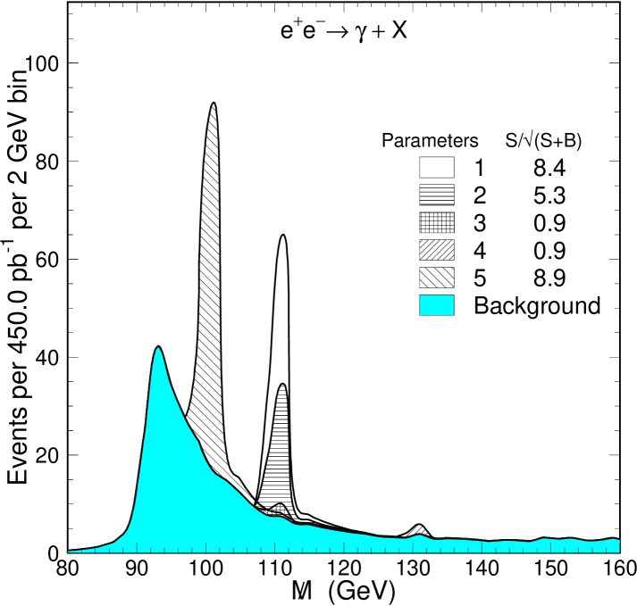
3a Anomaly Included

3b Anomaly Excluded

Figure 3: The recoil mass spectrum in ${\mathrm{{e^{+}}}\mathrm{{e^{-}}}}\to\mathrm{{\gamma}}\mathrm{{\Pi_{T}}}$ at $\sqrt{s}=200\,\mathrm{GeV}$ as simulated at the particle level in the TCSM using modifications to Pythia v6.202 as described in Section 3.2. In Figure 3a we display the background process, along with five different TCSM parameter sets: (1) The baseline set with $M_{V}=M_{A}=200\,\mathrm{GeV}$, $Q_{\mathrm{{U}}}+Q_{\mathrm{{D}}}=5/3$, $M_{\mathrm{{\Pi_{T}}}}=110\,\mathrm{GeV}$, and $M_{\mathrm{{\rho_{T}}}}=210\,\mathrm{GeV}$; (2) where $M_{V}=M_{A}=300\,\mathrm{GeV}$; (3) where $Q_{\mathrm{{U}}}+Q_{\mathrm{{D}}}=0$; (4) where $M_{\mathrm{{\rho_{T}}}}=250\,\mathrm{GeV}$ and $M_{\mathrm{{\Pi_{T}}}}=130\,\mathrm{GeV}$; and (5) where $M_{\mathrm{{\Pi_{T}}}}=100\,\mathrm{GeV}$. Figure 3b differs from Figure 3a in the exclusion of the anomaly coupling from the calculations. The legends display the signal to background significance ratios for each parameter set.

We now discuss our Pythia studies of the process ${\mathrm{{e^{+}}}\mathrm{{e^{-}}}}\to\mathrm{{\gamma}}\mathrm{{\Pi_{T}}}$ at the LEP collider. The kinematics of the process dictate that the photon is hard and more central than would be expected in background processes. We define the signal to be a significant peak in the “recoil mass” recoiling against the photon ${\makebox[0.0pt][l]{\hskip 2.89583pt$/$}{M}}=\sqrt{s-2\sqrt{s}E_{\mathrm{{\gamma}}}}$ for $E_{\mathrm{{\gamma}}}>10\,\mathrm{GeV}$ and $|\cos\theta_{\mathrm{{\gamma}}}|<0.7$. To reduce backgrounds, the photon must pass an isolation requirement: there must be no more than 5 GeV of excess energy within an opening angle of 30^∘ centered on the photon. Since the technipion is expected to decay visibly, and predominantly to $\mathrm{{b}}$ quarks, we will impose a $\mathrm{{b}}$–tag to eliminate the potentially large backgrounds from ${\mathrm{{e^{+}}}\mathrm{{e^{-}}}}\to\mathrm{{\gamma}}\mathrm{{\nu}}\smash[t]{\overline{\mathrm{{{\nu}}}}}$. We comment later on how to generalize this search.

We simulated the signal at the particle level using Pythia v6.202 [20], with updates to the technicolor simulation as specified in this paper. The proposed signature is a peak excess in the recoil mass distribution and a loose $\mathrm{{b}}$–tag in the rest of the event. We are not sure how stringent a $\mathrm{{b}}$–tag needs to be imposed and have not included any efficiency factors for the signal or fake rates from other quarks. We do not impose any kinematic cuts or jet–reconstruction algorithm on the particles recoiling from the photon, but require only a displaced vertex.

The only background included is from ${\mathrm{{e^{+}}}\mathrm{{e^{-}}}}\to\mathrm{{\gamma}}{\mathrm{{b}}\smash[t]{\overline{\mathrm{{{b}}}}}}$. To account for the final–state radiation of photons off the $\mathrm{{b}}$–partons, the full 2-to-3 parton–level process is calculated at the matrix element–level. The parton level calculation is then interfaced to Pythia, producing particle–level results that include the effects of parton showering and hadronization. After the isolation cut on the photon, the results are in good agreement with the standard Pythia simulation of ${\mathrm{{e^{+}}}\mathrm{{e^{-}}}}\to\mathrm{{\gamma}}+\mathrm{{\gamma}}^{*}/\mathrm{{Z^{*}}}$. The implied suppression of radiation off the $\mathrm{{b}}$–quark arises from several effects: (1) the small charge of the $\mathrm{{b}}$, (2) the large $\mathrm{{b}}$ quark mass, which regulates collinear emission, and (3) the kinematic constraints favoring a small invariant mass of the ($\mathrm{{b}}\mathrm{{\gamma}}$) or ($\smash[t]{\overline{\mathrm{{{b}}}}}\mathrm{{\gamma}}$) systems, which is removed by the isolation cut. Finally, we require that at least one of the $\mathrm{{b}}$–partons (after parton showering) has a $p_{T}$ of at least 5 GeV. Assuming that displaced vertices are detected with unit probability, this eliminates backgrounds from light quarks.

The results are shown in Figure 3a, assuming a collider energy of 200 GeV and $450\,\mathrm{pb^{-1}}$ of integrated luminosity. To demonstrate the variation with TCSM parameters, we have chosen five parameter sets starting with the baseline (1): $M_{V}=M_{A}=200\,\mathrm{GeV}$, $Q_{\mathrm{{U}}}+Q_{\mathrm{{D}}}=5/3$, $M_{\mathrm{{\Pi_{T}}}}=110\,\mathrm{GeV}$, and $M_{\mathrm{{\rho_{T}}}}=210\,\mathrm{GeV}$. The $\mathrm{{\mathrm{{\pi}}_{T}}}$ and $\mathrm{{\mathrm{{\pi}}_{T}^{\prime}}}$ and, separately, the $\mathrm{{\rho_{T}}}$ and $\mathrm{{\omega_{T}}}$ are assumed to be degenerate in mass. The other parameter sets are variations on this baseline, with all parameters as in (1) except: for (2), $M_{V}=M_{A}=300\,\mathrm{GeV}$; for (3), $Q_{\mathrm{{U}}}+Q_{\mathrm{{D}}}=0$; for (4), $M_{\mathrm{{\rho_{T}}}}=250\,\mathrm{GeV}$ and $M_{\mathrm{{\Pi_{T}}}}=130\,\mathrm{GeV}$; and, for (5), $M_{\mathrm{{\Pi_{T}}}}=100\,\mathrm{GeV}$. The general TCSM condition $Q_{U}-Q_{D}=1$ obtains for all parameter sets. Figure 3a shows also the significance defined as $S/\sqrt{S+B}$ for each of the parameter sets.

The baseline curve (1) includes a strong signal from the $\mathrm{{V_{T}}}$ poles just above the collider energy. Comparison with set (2) shows that the peak height scales as $M_{V}^{-2}$ as we would expect from Equation 2.11. Comparison with set (4), confirms the expected reduction of signal when the $\mathrm{{V_{T}}}$ and $\mathrm{{\Pi_{T}}}$ masses are scaled up to put the collider energy well below the poles. Set (3) allows us to infer that, as in figure 2, most of the $\mathrm{{V_{T}}}$ signal comes specifically from the $\mathrm{{\omega_{T}}}$. Taking $Q_{\mathrm{{U}}}+Q_{\mathrm{{D}}}=0$ decouples the $\mathrm{{\omega_{T}}}$ from the gauge bosons and eliminates the $\mathcal{V}_{\mathrm{{\gamma}}\mathrm{{\gamma}}\mathrm{{\Pi_{T}}}}$ coupling. The branching fraction for $\mathrm{{\rho_{T}}}\to\mathrm{{\gamma}}\mathrm{{\mathrm{{\pi}}_{T}^{\prime}}}$ is also small for these TCSM parameters, even though the $\mathrm{{\rho_{T}}}$ is kinematically forbidden to decay to a pair of $\mathrm{{\Pi_{T}}}$; the dominant decay is to $\mathrm{{W}}_{L}\mathrm{{\Pi_{T}}}$. Then the small signal in set (3) reflects the size of contributions from the $\mathcal{V}_{\mathrm{{\gamma}}\mathrm{{Z^{0}}}\mathrm{{\Pi_{T}}}}$ anomaly and the $\mathrm{{\rho_{T}}}\to\mathrm{{\gamma}}\mathrm{{\mathrm{{\pi}}_{T}}}$ channel. The only possible source of the much larger peak in set (1) is the restored contribution of the $\mathrm{{\omega_{T}}}$. Finally, in set (5), we deliberately open the (dominant when present) decay channel $\mathrm{{\rho_{T}}}\to\mathrm{{\Pi_{T}}}\mathrm{{\Pi_{T}}}$; this would normally be closed because of large extended technicolor contributions to the $\mathrm{{\Pi_{T}}}$ masses [13, 12]. Although this significantly decreases the $\mathrm{{\rho_{T}}}\to\mathrm{{\gamma}}\mathrm{{\Pi_{T}}}$ branching ratio, a strong signal of $\mathrm{{\omega_{T}}}\to\mathrm{{\gamma}}\mathrm{{\Pi_{T}}}$ still occurs because $\mathrm{{\omega_{T}}}$ decays to two or three $\mathrm{{\Pi_{T}}}$ remain suppressed or forbidden. Once again, the dominant role of the $\mathrm{{\omega_{T}}}$ in the signal is confirmed.

Figure 3b shows what the signals would look like if the anomaly couplings $\mathcal{V}_{\mathrm{{\gamma}}\mathrm{{\gamma}}\mathrm{{\Pi_{T}}}}$ and $\mathcal{V}_{\mathrm{{\gamma}}\mathrm{{Z^{0}}}\mathrm{{\Pi_{T}}}}$ were eliminated. The peak heights and significances are clearly reduced in all cases. For the parameter sets with the strongest signals (1,2,5), a comparison with figure 3a confirms that the $\mathrm{{\omega_{T}}}$ resonance is largely responsible for making the $\mathrm{{\Pi_{T}}}$ production visible. This is what we would expect from the results we presented in Figure 2, because the mass of the resonance is just slightly higher than the $\sqrt{s}$ of the collider. Nonetheless, the anomaly couplings make a contribution that can be large enough to impact the limits extracted from the data.

Several further comments are in order. First, the signature discussed here is strongly dependent on the $\mathrm{{\omega_{T}}}$ properties, especially the coupling $\mathrm{{\gamma}}\to\mathrm{{\omega_{T}}}\to\mathrm{{\gamma}}\mathrm{{\Pi_{T}}}$ which is proportional to $Q_{\mathrm{{U}}}+Q_{\mathrm{{D}}}$. In this respect, it is complementary to the $\mathrm{{\rho_{T}}}\to\mathrm{{W^{\pm}}}\mathrm{{\Pi_{T}}}$ signatures [8]. On the other hand, the TCSM may be naive in its assumption of certain mass degeneracies, and the $\mathrm{{\omega_{T}}}$ may be significantly lighter than the $\mathrm{{\rho_{T}}}$, yielding the first signature of technicolor. Second, the proposed signature is not inclusive, but assumes the $\mathrm{{\Pi_{T}}}\to{\mathrm{{b}}\smash[t]{\overline{\mathrm{{{b}}}}}}$ branching ratio is large (the observation of some visible energy is necessary to remove the $\mathrm{{\gamma}}+{\makebox[0.0pt][l]{\hskip 1.47916pt$/$}{E}}$ background). This is reasonable, but the solution to the flavor problem may bring surprises in the $\mathrm{{\mathrm{{\pi}}_{T}}}$ decay rates. There may also be a substantial rate for $\mathrm{{\mathrm{{\pi}}_{T}^{\prime}}}\to\mathrm{{g}}\mathrm{{g}}$ (this rate is already 30% for $\mathrm{{\mathrm{{\pi}}_{T}^{\prime}}}$ with the default TCSM choices as encoded in Pythia), and there even may be appreciable $\mathrm{{\mathrm{{\pi}}_{T}}}$–$\mathrm{{\mathrm{{\pi}}_{T}^{\prime}}}$mixing. Therefore, while the first search should be tuned for the $\mathrm{{\gamma}}{\mathrm{{b}}\smash[t]{\overline{\mathrm{{{b}}}}}}$ mode, we advocate a decay–independent search without the $\mathrm{{b}}$–tag. The background should be 4–5 times bigger, reducing $S/B$ (which is a few–to–one for the $\mathrm{{\gamma}}{\mathrm{{b}}\smash[t]{\overline{\mathrm{{{b}}}}}}$ signature). It will not not reduce the significance very much; we have defined it to include a systematic error on the background. For example, naively scaling the background estimate by 5 would reduce $S/\sqrt{S+B}$ to $6.6,3.7,0.4,0.5$, and $6.2$ for parameter sets $(1)$–$(5)$, respectively. This does not include the small increase in signal rate from all decays of the technipions.

4 Conclusions

In the context of the TCSM, we have shown that both the anomaly and kinetic mixing contributions should be included in analyses of technipion production at lepton colliders. We have provided analytic formulas combining these contributions and used them to display the predictions of the TCSM for a range of technihadron masses and collider energies. We have also performed Pythia simulations of ${\mathrm{{e^{+}}}\mathrm{{e^{-}}}}\to\mathrm{{\gamma}}\mathrm{{\Pi_{T}}}$ including the modifications to the TCSM described in this paper for five distinct sets of technihadron masses and technifermion charges. We find that resonant production of technipions is necessary to ensure a visible signature at LEP II energies for typical TCSM parameters, but that including the non-resonant production will be important for setting accurate limits. Finally, we note that measuring the recoil mass spectrum for ${\mathrm{{e^{+}}}\mathrm{{e^{-}}}}\to\mathrm{{\gamma}}\mathrm{{\Pi_{T}}}$ production (which we found to proceed mainly through the $\mathrm{{\omega_{T}}}$) provides a technicolor search strategy that is complementary to the $\mathrm{{\rho_{T}}}\to\mathrm{{W^{\pm}}}\mathrm{{\Pi_{T}}}$ channel.

Acknowledgments

We thank Guennadi Borisov and Francois Richard of DELPHI and Markus Schumacher of OPAL for asking questions that led to the present study and improvements in the TCSM. We are also grateful to R. Sekhar Chivukula and Markus Schumacher for comments on the manuscript. K. Lane acknowledges the support of the Fermilab Theory Group through a Frontier Fellowship. This work was also supported in part by the Department of Energy under grant DE-FG02-91ER40676 and by the National Science Foundation under grant PHY-0074274. FNAL is operated by Universities Research Association Inc. under contract DE-AC02-76CH03000.

References

- [1] S. Weinberg, Phys. Rev. D13, 974 (1976); S. Weinberg, Phys. Rev. D19, 1277 (1979); L. Susskind, Phys. Rev. D20, 2619 (1979).
- [2] B. Holdom, Phys. Rev. D24, 157 (1981).
- [3] E. Eichten and K. D. Lane, Phys. Lett. B90, 125 (1980); B. Holdom, Phys. Rev. D24, 1441 (1981); B. Holdom, Phys. Lett. B150, 301 (1985); T. W. Appelquist, D. Karabali, and L. C. R. Wijewardhana, Phys. Rev. Lett. 57, 957 (1986); T. Appelquist and L. C. R. Wijewardhana, Phys. Rev. D36, 568 (1987); K. Yamawaki, M. Bando, and K.-i. Matumoto, Phys. Rev. Lett. 56, 1335 (1986); T. Akiba and T. Yanagida, Phys. Lett. B169, 432 (1986).
- [4] C. T. Hill, Phys. Lett. B266, 419 (1991); C. T. Hill, Phys. Lett. B345, 483 (1995), hep-ph/9411426.
- [5] K. D. Lane and E. Eichten, Phys. Lett. B222, 274 (1989); K. D. Lane and M. V. Ramana, Phys. Rev. D44, 2678 (1991).
- [6] E. Eichten and K. D. Lane, Phys. Lett. B388, 803 (1996), hep-ph/9607213.
- [7] E. Eichten, K. D. Lane, and J. Womersley, Phys. Rev. Lett. 80, 5489 (1998), hep-ph/9802368.
- [8] E. Eichten, K. D. Lane, and J. Womersley, Phys. Lett. B405, 305 (1997), hep-ph/9704455.
- [9] T. Affolder et al. (CDF) (1999), FERMILAB-PUB-99-141-E; F. Abe et al. (CDF), Phys. Rev. Lett. 83, 3124 (1999), hep-ex/9810031; T. Affolder et al. (CDF), Phys. Rev. Lett. 84, 1110 (2000); T. Affolder et al. (CDF), Phys. Rev. Lett. 85, 2056 (2000), hep-ex/0004003; F. Abe et al. (CDF), Phys. Rev. Lett. 82, 3206 (1999).
- [10] J. Abdallah et al. (DELPHI), Eur. Phys. J. C22, 17 (2001), hep-ex/0110056; The OPAL Collaboration, Searches for Technicolor with the OPAL Detector in e+e- Collisions at the Highest LEP Energies (2001), OPAL Physics Note PN485.
- [11] K. R. Lynch and E. H. Simmons, Phys. Rev. D64, 035008 (2001), hep-ph/0012256.
- [12] K. D. Lane (1999), hep-ph/9903372.
- [13] K. D. Lane, Phys. Rev. D60, 075007 (1999), hep-ph/9903369.
- [14] A. Manohar and L. Randall, Phys. Lett. B246, 537 (1990).
- [15] L. Randall and E. H. Simmons, Nucl. Phys. B380, 3 (1992).
- [16] S. Dimopoulos, S. Raby, and G. L. Kane, Nucl. Phys. B182, 77 (1981); J. R. Ellis, M. K. Gaillard, D. V. Nanopoulos, and P. Sikivie, Nucl. Phys. B182, 529 (1981).
- [17] G. Rupak and E. H. Simmons, Phys. Lett. B362, 155 (1995), hep-ph/9507438.
- [18] R. Casalbuoni, A. Deandrea, S. D. Curtis, D. Dominici, R. Gatto, and J. F. Gunion (1999), hep-ph/9912333; V. Lubicz and P. Santorelli, Nucl. Phys. B460, 3 (1996), hep-ph/9505336.
- [19] R. W. Brown and K. O. Mikaelian, Phys. Rev. D19, 922 (1979).
- [20] T. Sjostrand et al., Comput. Phys. Commun. 135, 238 (2001), hep-ph/0010017; T. Sjostrand, L. Lonnblad, and S. Mrenna (2001), hep-ph/0108264.