Abstract

In view of their physics goals, future neutrino factories from muon decay aim at an overall flux precision of ${\cal O}(1\%)$ or better. We analytically study the QED radiative corrections to the neutrino differential distributions from muon decay. Kinematic uncertainties due to the divergence of the muon beam are considered as well. The resulting corrections to the neutrino flux turn out to be of order ${\cal O}(0.1\%)$, safely below the required precision.

1 Introduction

Results on neutrino oscillations from Superkamiokande [1] and SNO [2] provide a compelling evidence for neutrino masses, constituting the first strong indication of Physics beyond the Standard Model. Much is still unknown, though, regarding fundamental issues such as the absolute neutrino mass scale, the possible Majorana character of neutrino fields, the ordering of their mass eigenstates with respect to charged lepton eigenstates, or the possible existence of leptonic CP violation and its tantalizing relationship to baryogenesis. In this situation one could argue that the subject of lepton flavor physics is at its exciting infancy, and to obtain rough answers to those questions could be a sufficient goal at present, postponing any aim at a precise determination of the involved parameters. Nevertheless, some of those questions prerequire precision: for instance the study of CP violation rests upon a precise knowledge of the angles in the neutrino mixing matrix.

In a more general way and much as for the quark sector, it is necessary to know accurately the values of the masses and mixing parameters in the lepton sector, as a first step to unravel the flavor puzzle. And what does precision means, quantitatively?. For instance, with which precision is it desirable to determine the values of the leptonic mixing angles in order to discriminate between models for neutrino masses? Clearly no definite answer can be given to such question, but as an indication it has been argued [4] that a $10\%-1\%$ precision in the knowledge of, say, $sin^{2}2\theta_{atm}$ would result in significant advance. It is not impossible to envisage such a precision. In resume, we are simultaneously entering a discovery and a precision era in neutrino physics. With the bonus that the extraction of physical conclusions will not be necessarily hindered by large theoretical errors, as it happens in the quark sector due to QCD long distance contributions.

A quest for precise physics answers evidently requires an effort in precision on the experimental conditions, and on the knowledge of the neutrino flux to start with. Several experiments using neutrino beams from particle accelerators such as K2K, MINOS and OPERA [3] will take data in the next few years. Their reach will be limited by the use of conventional neutrino beams produced from a charged pion source. The decay $\pi^{+}\rightarrow\mu^{+}\nu_{\mu}\,(\pi^{-}\rightarrow\mu^{-}\bar{\nu}_{\mu})$ produces a $\nu_{\mu}$ beam with a ${\cal O}(1\%)$ component of $\nu_{e}$ from kaon decays. The $\nu_{e}$ contamination limits the precision of the flux measurements, resulting in an error of $7\%$ for K2K, while MINOS reduces it to $2\%$ [3]. A further step forward could be provided by the so-called superbeams which, although based on the same traditional beams, can achieve better precision thanks to the much higher statistics. It has been argued, for example, that by working at energies below the threshold of kaon production, the $\nu_{e}$ flavor contamination could be reduced, with the overall figure of merit for precision in the flux measurements limited to ${\cal O}(1\%)$ [6, 7].

A major advance should come from a neutrino factory from muon decays, aiming at both fundamental discoveries and ${\cal O}(1\%)$ precision measurements. Present projects consider the production of very intense muon sources of about $10^{20}$ muons per year [8]. Neutrino beams originate from the decay of high-momentum muons along the straight sections of a storage ring. The beam produced presents a precisely known neutrino content: $50\%$ muon neutrinos and $50\%$ electron antineutrinos if a $\mu^{-}$ beam is used, and $50\%$ muon antineutrinos and $50\%$ electron neutrinos if a $\mu^{+}$ beam is used. The resulting $\nu$ fluxes are expected to be known with a precision better than $1\%$ [9]. It is necessary to ensure that any possible corrections and sources of errors are controlled at that level. In this work, we study two effects: the contribution of QED one-loop corrections to muon decay and the divergence of the muon beam. For both cases, we give novel corrected formulae for neutrino differential distributions.

Radiative corrections to the electron differential distribution in $\mu^{-}\rightarrow e^{-}+\bar{\nu}_{e}+\nu_{\mu}$ were calculated long ago resulting in a correction of ${\cal O}(1\%)$ [10], larger than the expected effect of ${\cal O}(\frac{\alpha}{\pi})\sim{\cal O}(0.1\%)$. Such an effect is at the level of the expected precision at a neutrino factory. In this work we study whether QED corrections affect neutrino distributions at the same order.

The correction to the (massive) neutrino spectra from unpolarized muons has been first calculated in [11]. In our work, we give new anlytic formulae with $m_{\nu}=0$ and $m_{e}=0$ including muon polarization, relevant for neutrino factory measurements. Different from the electron case, the analysis of the correction to the neutrino differential distributions entails non-trivial integrations. By using the correspondence between the QED corrections to the $\mu$-decay and those for the charge $2/3$ heavy quarks in QCD, we make use of the techniques developped in Refs. [12, 13, 14] for the calculation of the QCD corrections to the lepton spectrum in the decay $t\rightarrow b+l^{+}+\nu_{l}$.

The second subject addressed in this paper is that of the muon beam divergence, one of the basic properties that can bias the predicted neutrino spectra . We explore the error induced in the neutrino distributions at the far site due to the systematic uncertainty on the angular divergence, and compare our results with previous ones in which this effect was not included [15].

The paper is organized as follows. In section 2 we recall the tree-level angular distributions. In section 3 the neutrino one-loop corrected formulae are given, with 3.1 specializing in the soft photon limit and cancellation of infrared divergences. Section 4 accounts for the corrections due to the beam divergence.

2 General definitions

In the muon rest-frame, the angular distributions of the neutrinos produced in the decay $\mu^{-}\rightarrow e^{-}+\nu_{\mu}+\bar{\nu}_{e}$, Fig. 1a, are computed from the muon decay rate:

$$d\Gamma_{0}=\frac{1}{2m_{\mu}}\,64\,{\rm G_{F}}^{2}\,\,|M_{0}(p_{\mu};p_{e},p_{\bar{\nu}_{e}},p_{\nu_{\mu}})|^{2}\,d\Phi_{3}(p_{\mu};p_{e},p_{\bar{\nu}_{e}},p_{\nu_{\mu}})~{},$$ (1)

where $|M_{0}(p_{\mu},p_{e},p_{\bar{\nu}_{e}},p_{\nu_{\mu}})|^{2}$ is the averaged squared amplitude obtained from the Feynmann diagram at tree level. For polarized muons:

$$|M_{0}(p_{\mu};p_{e},p_{\bar{\nu}_{e}},p_{\nu_{\mu}})|^{2}=\left[(p_{\mu}-m_{\mu}s)\,p_{\bar{\nu}_{e}}\right](p_{e}p_{\nu_{\mu}})~{},$$ (2)

where $s$ is the four-spin. For unpolarized muons $s=0$.

$d\Phi_{3}$ is the three-body phase-space. In general, the n-body phase space is defined by :

$$d\Phi_{n}(P;p_{1},...,p_{n})=(2\pi)^{4}\,\delta(P-p_{1}-...-p_{n})\,\prod_{i=1}^{n}\frac{d^{3}{\bf p_{i}}}{2p_{i}^{0}}\frac{1}{(2\pi)^{3}}~{}.$$ (3)

Differential distributions of decay products are obtained integrating over the phase space of the remaining decay particles,

$$\frac{d^{2}N}{dx\,d\cos{\theta}}=F^{(0)}(x)+J^{(0)}(x)\,{\cal P}_{\mu}\cos\theta~{},$$ (4)

where $x$ denotes the scaled energy, $x=2E_{e,\nu}/m_{\mu}$ and ${\cal P}_{\mu}$ is the average over polarization of the initial state muon along the beam direction. $\theta$ is the angle between three-momentum of the emitted particle and the muon spin direction and $m_{\mu}$ is the muon mass. The normalized functions $F^{(0)}$ and $J^{(0)}$, in the limit $m_{e}=0$, read [16]:

$$F_{e}^{(0)}(x) = x^{2}(3-2x)~{},\qquad J_{e}^{(0)}(x)=x^{2}(1-2x)~{},$$ (5)

$$F_{\nu_{\mu}}^{(0)}(x) = x^{2}(3-2x)~{},\qquad J_{\nu_{\mu}}^{(0)}(x)=x^{2}(1-2x)~{},$$ (6)

$$F_{\bar{\nu}_{e}}^{(0)}(x) = 6x^{2}(1-x)~{},\qquad J_{\bar{\nu}_{e}}^{(0)}(x)=6x^{2}(1-x)~{}.$$ (7)

3 QED corrections

The QED radiative corrections to the formula (5) where calculated long ago in Ref. [10] through the integration over the neutrino phase-space of the $\cal{O}(\alpha)$ corrected differential muon decay rate. The QED corrections to the Eq. (6) ( Eq. (7) ), are similarly obtained from the integration over the $\bar{\nu}_{e}-e^{-}$ ($\nu_{\mu}-e^{-}$) phase-space.

In the muon decay, the QED corrected differential rate is given by

$${\rm d}\Gamma={\rm d}\Gamma_{0}+{\rm d}\Gamma_{V}+{\rm d}\Gamma_{R}~{},$$ (8)

where ${\rm d}\Gamma_{V}$ describes the contribution of virtual photon diagrams in Figs. 1b-1d and ${\rm d}\Gamma_{R}$ accounts for the effects of the real photon emission diagrams in Fig. 1e and Fig. 1f.

The virtual photon correction to the decay rate is given by

$$d\Gamma_{V}=\frac{1}{2m_{\mu}}\,64\,{\rm G_{F}}^{2}\,\,|M_{V}|^{2}\,d\Phi_{3}(p_{\mu};p_{e},p_{\bar{\nu}_{e}},p_{\nu_{\mu}})~{},$$ (9)

where $|M_{V}|^{2}$ is the squared amplitude. For unpolarized muons it has the expression:

$$|M_{V}|^{2}=|M_{0}|^{2}\,-\,\frac{\alpha}{\pi} \bigg{[} g_{\rm{L}}^{\rm{S}}\,|M_{0}|^{2}+\frac{m_{\mu}m_{e}}{4}\,g_{\rm{R}}^{\rm{S}}\,(p_{\bar{\nu}_{e}}p_{\nu_{\mu}})$$ (10)

$$+ m_{e}\,g_{\rm{L}}^{\rm{V}}\,(p_{\mu}p_{\bar{\nu}_{e}})(p_{\mu}p_{\nu_{\mu}})+m_{\mu}\,g_{\rm{R}}^{\rm{V}}\,(p_{e}p_{\bar{\nu}_{e}})(p_{e}p_{\nu_{\mu}})\,\,\bigg{]}~{}.$$

where $g_{\,\rm{L,R}}^{\rm{S,V}}$ are ultraviolet (UV) and are listed in the appendix A. The function $g_{\rm{L}}^{S}$ is infrared (IR) divergent while the rest of the “$g$” functions are finite.

The IR singularity in $g_{\rm{L}}^{S}$ is canceled with the soft photon terms of the real emission diagrams, which correct the differential rate as

$$d\Gamma_{R}=\frac{1}{2m_{\mu}}\,64\,{\rm G_{F}}^{2}\,\,|M_{R}|^{2}\,d\Phi_{4}(p_{\mu};p_{e},p_{\bar{\nu}_{e}},p_{\nu_{\mu}},k)~{}.$$ (11)

The explicit expression of the amplitude $|M_{R}|^{2}$ can be found in the Appendix A.

QED corrections for polarized muons are calculated identically to those of unpolarized ones with the replacement $p_{\mu}\rightarrow p_{\mu}-sm_{\mu}$ in the amplitudes , where $s$ is the muon four-spin [13].

3.1 Soft photon limit and IR cancellation

Before continuing with the discussion of the exact corrections, let us consider their soft photon limit, i.e. $k\rightarrow 0$, as only IR singular terms of virtual and real photon diagrams remain in this limit. When soft virtual and soft real photon contributions are added up, all ${\cal O}(\alpha)$ IR singularities are canceled.

In this limit, the ${\cal O}(k)$ terms in the virtual photon diagrams are neglected and Eq. (10) is simplified to :

$$|M_{V}^{\rm SP}|^{2}=\left(1-\,\frac{\alpha}{\pi}\,g_{\rm{L}}^{\rm{S}}\right)\,|M_{0}|^{2},$$ (12)

where $g_{\rm{L}}^{\rm{S}}$ contains all IR divergent terms which are regularized introducing a finite photon mass $\lambda$.

In the diagrams containing real photon emission, only terms of order ${\cal O}(k^{-2})$ remain in the soft photon limit. They contain all IR divergent contributions from bremsstrahlung. The squared amplitude in Eq.(11) reduces to:

$$|M_{R}^{\rm SP}|^{2}=32\,\frac{\alpha}{2\pi}\,\bigg{[}\frac{p_{\mu}^{2}}{(p_{\mu}k)^{2}}+\frac{p_{e}^{2}}{(p_{e}k)^{2}}-\frac{2(p_{\mu}p_{e})}{(p_{\mu}k)(p_{e}k)}\bigg{]}|M_{0}|^{2}.$$ (13)

The divergences in Eq. (12) cancel when added with the soft bremsstrahlung part. However, Eq. (13) must be previously integrated over the photon-electron phase space in order to reduce the real phton emission from a four-body problem to a three-body problem. The integral is performed introducing a finite photon mass $\lambda$, resulting in a expression which exactly cancels the IR terms in Eq. (12).

After the integration over the corresponding phase space, we obtain the soft-photon corrected for both $\nu_{\mu}$ and $\bar{\nu}_{e}$ distributions, which are proportional to the tree level amplitude , in the limits $x\rightarrow 1$ and $m_{e}\rightarrow 0$:

$$\frac{d^{2}N_{\nu}^{SP}}{dx\,d\cos{\theta}}=F_{\nu}^{(0)}(x)[1-\frac{\alpha}{2\pi}\,k(x)].$$ (14)

The resulting function $k(x)$ is $\lambda$-independent:

$$k(x)=2\,{\rm L}(x)+2\pi^{2}/3+\ln^{2}(1-x).$$ (15)

where ${\rm L}(x)$ is the Spence function defined in the Appendix A.

Realize that $k(x)$ diverges for $x\rightarrow 1$. This singularity is originated due to a failure the perturbative treatment: at the end point of the spectrum, the phase space for the emission of real photons shrinks to zero and does not compensate the IR infinities of the virtual photons.

The end-point singularity of the corrected electron distribution from muon decay has been largely discussed in the literature [17]. For $x\rightarrow 1$ and $k\rightarrow 0$, the corrected electron differential distribution diverges as $\ln(1-x)$. Since the IR divergences in the muon decay stem from soft-photons in the limit $k\rightarrow 0$, the solution proposed to control the end-point divergence is to consider multiple soft-photon emission. The effect of considering soft photons at all orders in $\alpha$ is the exponentiation of the singular logarithm $\ln(1-x)$ which leads to a non-singular distribution [18].

Following as a guideline the solution found for the electron, we apply the same proccedure to the neutrino distributions. Consider the neutrino soft-photon correction in Eq. (14). At the end-point, for each soft virtual photon and each soft real photon we get a $\ln^{2}(1-x)$ term, which multiplies the tree level amplitude. If there are $n$ soft virtual photons and $n$ soft real photons, there are $n$ double logarithms with an additional symmetry factor of $1/n!$. Therefore, the correction to the neutrino distribution at all orders in $\alpha$ is obtained summing over $n$:

$$\frac{d^{2}N_{\nu}}{dx\,d\cos{\theta}}=[F_{\nu}^{(0)}(x)+J_{\nu}^{(0)}\,{\cal P}_{\mu}(x)\cos\theta]\,e^{-\frac{\alpha}{2\pi}\ln^{2}(1-x)}~{}.$$ (16)

The evaluation of infrared divergences at all orders results in the exponentiation of the double logarithm, which ensures a non-divergent behavior of the neutrino distributions. The exponentiation is only valid for a small region $x\rightarrow 1$. For lower $x$, we must include all the terms of the exact corrections, computed in the next subsection.

3.2 Results

Exactly corrected neutrino distributions are obtained considering all terms of the ${\cal O}(\alpha)$ corrected decay rate, Eq. (8) and integrating over the phase space of the remaining particles. Different from the corrected electron distribution, in the neutrino case, the integrals over the electron-photon phase space in the real emission diagrams are nontrivial. We follow the method found in Ref. [14] to solve analytically these integrals in the calculation of the QCD corrections to the lepton spectrum from the decay $t\rightarrow b+l^{+}+\nu_{l}$. We use the fact that there is a one to one correspondence between the Feynmann diagrams in Fig. 1 for the QED corrections to the $\mu$-decay and those for the top quarks. This correspondence can be seen by simply replacing

$$\alpha \to \frac{4}{3}\alpha_{S}$$

$$(\mu^{-},e^{-},\bar{\nu}_{e},\nu_{\mu}) \to (t,b,l^{+},\nu_{l})~{}.$$ (17)

Therefore, by following the techniques detailed Ref. [14], we perform the corresponding phase-space integrals to the differential rate of polarised muons. We find that the corrected neutrino angular and energy distributions, including all finite terms in the limit $m_{e}=0$, are:

$$\frac{d^{2}N_{\nu_{\mu}}}{dx\,d\cos{\theta}}=F_{\nu_{\mu}}^{(0)}(x)+J_{\nu_{\mu}}^{(0)}\,{\cal P}_{\mu}(x)\cos\theta-\frac{\alpha}{2\pi}\left[F_{\nu_{\mu}}^{(1)}(x)+J_{\nu_{\mu}}^{(1)}(x)\,{\cal P}_{\mu}\cos\theta\right]\,\,,$$

$$\frac{d^{2}N_{\bar{\nu}_{e}}}{dx\,d\cos{\theta}}=F_{\bar{\nu}_{e}}^{(0)}(x)+J_{\bar{\nu}_{e}}^{(0)}(x)\,{\cal P}_{\mu}\cos\theta-\frac{\alpha}{2\pi}\left[F_{\bar{\nu}_{e}}^{(1)}(x)+J_{\bar{\nu}_{e}}^{(1)}(x)\,{\cal P}_{\mu}\cos\theta\right]\,\,$$ (18)

where $F_{{\bar{\nu}_{e}},\nu_{\mu}}^{(0)}$-$J_{{\bar{\nu}_{e}},\nu_{\mu}}^{(0)}$ are given in Eq. (6), and the one-loop corrections are given by:

$$F_{\nu_{\mu}}^{(1)}(x) = F_{\nu_{\mu}}^{(0)}(x)k(x)+\frac{1}{6}(41-36x+42x^{2}-16x^{3})\ln(1-x)$$ (19)

$$+ \frac{1}{12}x(82-153x+86x^{2})\,\,,$$

$$J_{\nu_{\mu}}^{(1)}(x) = J_{\nu_{\mu}}^{(0)}(x)k(x)+\frac{1}{6}(11-36x+14x^{2}-16x^{3}-4/x)\ln(1-x)$$ (20)

$$+ \frac{1}{12}(-8+18x-103x^{2}+78x^{3})\,\,,$$

$$F_{\bar{\nu}_{e}}^{(1)}(x) = F_{\bar{\nu}_{e}}^{(0)}(x)k(x)+(1-x)\Big{[}(5+8x+8x^{2})\ln(1-x)$$ (21)

$$+ \frac{1}{2}x(10-19x)\Big{]}\,\,,$$

$$J_{\bar{\nu}_{e}}^{(1)}(x) = J_{\bar{\nu}_{e}}^{(0)}(x)k(x)+(1-x)\Big{[}(-3+12x+8x^{2}+4/x)\ln(1-x)$$ (22)

$$+ \frac{1}{2}(8-2x-15x^{2})\Big{]}\,\,.$$

As expected, due to the above correspondence, the results in Eqs. (19)-(22) are identical to those for the QCD corrections of the lepton distributions from top decay.

Notice that the function $k(x)$ appears in Eqs. (19)-(22) multiplying the tree level functions $F_{\nu}^{(0)}$-$J_{\nu}^{(0)}$, which agrees with the discussion in the former subsection.

Fig. 2 and Fig. 4 compare the corrected and the tree level forward $\nu_{\mu}$ and $\nu_{e}$ distributions, respectively. In both cases, the relative correction is of ${\cal O}(0.1\%)$, well below the order of the expected precision in the knowledge of the beam parameters.

The correction found of ${\cal O}(\frac{\alpha}{\pi})\sim{\cal O}(0.1\%)$ agrees of that expected from first order QED processes. This result differs with the correction of ${\cal O}(1\%)$ found for the electron distribution [10]. The enhacement of the correction the $e^{-}$ case is due to the “leading logs”: terms proportional to $\ln(\frac{m_{\mu}}{m_{e}})$ which stem from the emission of collinear photons in the electron leg [19]. Since neutrinos are not sensitive to QED, no term in $\frac{\alpha}{\pi}\ln(\frac{m_{\mu}}{m_{\nu}})$ appears in the neutrino distributions and, neither, terms in $\frac{\alpha}{\pi}\log(\frac{m_{\mu}}{m_{e}})$, which cancel when the variables affected by QED corrections, i.e. electron and the photon electron momenta, are integrated over. An identical cancellation it is found in the ${\cal O}({\alpha})$ corrections to the muon lifetime computed which result to be of ${\cal O}(\frac{\alpha}{\pi})\sim{\cal O}(0.1\%)$ [10].

In the laboratory frame, neutrino fluxes are boosted along the muon momentum direction. The formulae of the corrected distributions in that frame are given in Appendix B.

4 Muon-beam divergence

We study below the systematic uncertainty in the neutrino distributions produced by the muon beam divergence. For the sake of illustration, the quantitative results will be given for a $30$ GeV unpolarized muon beam decaying in a long straight section pointing to a far detector located at $2810$ km.

The natural decay angle of the forward neutrino beam in the laboratory frame is deduced from the relation between the rest and laboratory frames. In the rest frame, half of the neutrinos are emitted within the cone $\theta\leq\pi/2$. In the laboratory frame:

$$\cos\theta^{{}^{\prime}}=\frac{\cos\theta+\beta}{1+\beta\cos\theta},$$ (23)

where $\beta=\sqrt{1-\gamma^{-2}}$ is the muon velocity in the laboratory frame. Therefore, half of neutrinos are emitted within the cone subtended by the decay angle $\theta^{{}^{\prime}}\leq 1/\gamma$. For instance, for $30$ GeV muons $1/\gamma=m_{\mu}/E_{\mu}=3$ mrad.

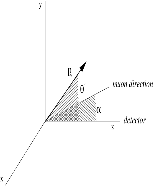
Figure 6: Muon divergence in the laboratory frame

For the beam and baseline illustrated here, a $10$ kt detector and one year of data taking [20], the statistical error on the neutrino flux is of the order of O($0.4\%$). It is then convenient to restrain the uncertainty induced by the muon beam divergence below that level. To achieve this, the direction of the beam must be carefully monitored within the decay straight section by placing beam position monitors at its ends. The angular divergence of the parent muon beam is then small compared to the natural decay angle of the neutrino beam $\theta^{{}^{\prime}}\sim 1/\gamma$, see Fig. 6, aiming at present to a divergence of ${\cal O}(0.1/\gamma)$. It implies that the neutrino beam will be collinear, within the limits set by the decay kinematics.

In our calculations we parameterize this beam focalization by a gaussian distribution with standard deviation $\sigma\sim 0.1/\gamma$ (i.e. $0.3$ mrad for $30$ GeV muon beam) [21], which suppresses the flux of neutrinos as they separate from the straight direction. The divergence is introduced analytically by considering that the muon direction opens an angle $\alpha$ with respect to the z-axis, defined as the direction pointing towards the far detector at a distance $L$, see Fig. 6. The neutrino distributions in the rest frame, Eq. (4), are Lorentz boosted along the z-axis. The rest-frame basis $(x,\cos{\theta})$ is transformed to the lab-frame basis $(z,\cos{\theta}^{{}^{\prime}})$, where $z=E_{\nu}/E_{\mu}$ and $\theta^{{}^{\prime}}$ is the angle between the neutrino beam and the z-axis. Using the parameters $\beta=\sqrt{1-\gamma^{-2}}$, the boosted distributions read:

$$\frac{d^{2}N_{\bar{\nu}_{\mu},\nu_{\mu}}}{dzd\Omega} = \frac{4n_{\mu}}{\pi L^{2}m_{\mu}^{6}}\,E_{\mu}^{4}z^{2}(1-\beta(\sin\varphi^{{}^{\prime}}\sin\alpha\sin\theta^{{}^{\prime}}+\cos\alpha\cos\theta^{{}^{\prime}}))$$

$$\times\left\{\left[3m_{\mu}^{2}-4zE_{\mu}^{2}(1-\beta(\sin\varphi^{{}^{\prime}}\sin\alpha\sin\theta^{{}^{\prime}}+\cos\alpha\cos\theta^{{}^{\prime}}))\right]\right.$$

$$\left.\mp\,{\cal P}_{\mu}\left[m_{\mu}^{2}-4z(1-\beta(\sin\varphi^{{}^{\prime}}\sin\alpha\sin\theta^{{}^{\prime}}+\cos\alpha\cos\theta^{{}^{\prime}}))\right]\right\},\,$$

$$\frac{d^{2}N_{\nu_{e},\bar{\nu}_{e}}}{dzd\Omega} = \frac{24n_{\mu}}{\pi L^{2}m_{\mu}^{6}}\,E_{\mu}^{4}z^{2}(1-\beta(\sin\varphi^{{}^{\prime}}\sin\alpha\sin\theta^{{}^{\prime}}+\cos\alpha\cos\theta^{{}^{\prime}}))$$ (24)

$$\times\left\{\left[m_{\mu}^{2}-2zE_{\mu}^{2}(1-\beta(\sin\varphi^{{}^{\prime}}\sin\alpha\sin\theta^{{}^{\prime}}+\cos\alpha\cos\theta^{{}^{\prime}}))\right]\right.$$

$$\left.\mp\,{\cal P}_{\mu}\left[m_{\mu}^{2}-4z(1-\beta(\sin\varphi^{{}^{\prime}}\sin\alpha\sin\theta^{{}^{\prime}}+\cos\alpha\cos\theta^{{}^{\prime}}))\right]\right\}.$$

The above expressions are integrated on $\alpha$, weighted with the gaussian factor

$$\frac{e^{\frac{-\alpha^{2}}{2\sigma^{2}}}}{\sqrt{2\pi\sigma^{2}}}.$$ (25)

For unpolarized muons ($P_{\mu}=0$) (for different muon polarizations we obtain similar results), it results:

$$\frac{d^{2}N_{\bar{\nu}_{\mu},\nu_{\mu}}}{dzd\Omega} = \frac{4n_{\mu}}{\pi L^{2}m_{\mu}^{6}}\,E_{\mu}^{4}z^{2}\,\left\{3m_{\mu}^{2}\left(1-\beta e^{\frac{-\sigma^{2}}{2}}\cos\theta^{{}^{\prime}}\right)\right.$$

$$\left.-4zE_{\mu}^{2}\left(1-2\beta e^{\frac{-\sigma^{2}}{2}}\cos\theta^{{}^{\prime}}\right.\right.$$

$$\left.\left.+\beta^{2}\left(\frac{1-e^{-2\sigma^{2}}}{2}\right)\sin^{2}\theta^{{}^{\prime}}\sin^{2}\varphi^{{}^{\prime}}+\beta^{2}\left(\frac{1+e^{-2\sigma^{2}}}{2}\right)\cos^{2}\theta^{{}^{\prime}}\right)\right\},$$

$$\frac{d^{2}N_{\nu_{e}\bar{\nu}_{e}}}{dzd\Omega} = \frac{24n_{\mu}}{\pi L^{2}m_{\mu}^{6}}\,E_{\mu}^{4}z^{2}\,\left\{m_{\mu}^{2}\left(1-\beta e^{\frac{-\sigma^{2}}{2}}\cos\theta^{{}^{\prime}}\right)\right.$$ (26)

$$\left.-2zE_{\mu}^{2}\left(1-2\beta e^{\frac{-\sigma^{2}}{2}}\cos\theta^{{}^{\prime}}\right.\right.$$

$$\left.\left.+\beta^{2}\left(\frac{1-e^{-2\sigma^{2}}}{2}\right)\sin^{2}\theta^{{}^{\prime}}\sin^{2}\varphi^{{}^{\prime}}+\beta^{2}\left(\frac{1+e^{-2\sigma^{2}}}{2}\right)\cos^{2}\theta^{{}^{\prime}}\right)\right\}.$$

Setting $\theta^{{}^{\prime}}=0$, the expression of forward neutrino fluxes reads:

$$\frac{d^{2}N_{\bar{\nu}_{\mu},\nu_{\mu}}}{dzd\Omega} = \frac{4n_{\mu}}{\pi L^{2}m_{\mu}^{6}}\,E_{\mu}^{4}z^{2}\,\left\{3m_{\mu}^{2}\left(1-\beta e^{\frac{-\sigma^{2}}{2}}\right)\right.$$

$$\left.-4zE_{\mu}^{2}\left(1-2\beta e^{\frac{-\sigma^{2}}{2}}+\beta^{2}\left(\frac{1+e^{-2\sigma^{2}}}{2}\right)\right)\right\},$$

$$\frac{d^{2}N_{\nu_{e}\bar{\nu}_{e}}}{dzd\Omega} = \frac{24n_{\mu}}{\pi L^{2}m_{\mu}^{6}}\,E_{\mu}^{4}z^{2}\,\left\{m_{\mu}^{2}\left(1-\beta e^{\frac{-\sigma^{2}}{2}}\right)\right.$$ (27)

$$\left.-2zE_{\mu}^{2}\left(1-2\beta e^{\frac{-\sigma^{2}}{2}}+\beta^{2}\left(\frac{1+e^{-2\sigma^{2}}}{2}\right)\right)\right\}.$$

Figs. 7, 8 show the numerical results for the neutrino and antineutrino spectra in a medium baseline ($2810$ km). We compare the distribution where the muon beam is aligned with the detector direction (no beam divergence) with the distribution where the muon-beam divergence is included. In the former, neutrino beams are averaged over an angle $\theta^{{}^{\prime}}$ of $0.1$ mrad at the far detector [15].

Our formulae predict a similar flux correction than previous numerical estimations [21]. For instance, a $10\%$ uncertainty in the muon beam divergence would lead to a flux uncertainty of $0.3\%$. We obtain,

$$\frac{\frac{\Delta dN_{\nu}}{dE}}{\frac{dN_{\nu}}{dE}}\sim 0.03\frac{\Delta\alpha}{\alpha}.$$ (28)

If the muon beam divergence is constrained by lattice design to be less than $0.05/\gamma$, the loss of flux will be negligible [22].

5 Conclusions

A neutrino factory from muon decay aims at a precision better than ${\cal O}(1\%)$ in the knowledge of the resulting intense neutrino fluxes.

We have presented here novel results about the effects of QED corrections and muon beam divergence on the neutrino differential distributions from muon decay. We have given the corresponding corrected formulae (for $m_{e}=0$ and $m_{\nu}=0$), including muon polarization effects. The induced uncertainties on the neutrino spectra turn out to be a safe ${\cal O}(0.1\%)$.

Neutrino one-loop corrected distributions diverge at the upper edge of the kinematical allowed region. This results from a failure in the cancellation of infrared divergences from virtual photons by real photons. Applying the soft photon limit to the exact calculations, we have isolated the end-point divergent term for the neutrino distributions which takes the form of $\ln^{2}(1-x)$. In order to control this singularity, the double logarithmic-contribution is exponentiated, encompassing the contributions from all orders of perturbation theory. All in all, the exact neutrino distributions get corrections of ${\cal O}(0.1)\%$, safely below the expected precision in the flux measurements.

We have also studied carefully the influence of the muon beam divergence on the neutrino spectra at the far site. The challenge in designing the neutrino production section, where the muons decay, is to constrain the muon beam divergence to a value smaller than the natural cone of forward going neutrinos in the laboratory frame, ($\sim 1/\gamma$). At present, the long straight sections under discussion aim at an angular muon beam divergence of the order of $0.1/\gamma$, typically less than one mrad.

6 Acknowledgments

We thank M.B. Gavela, P. Hernández and A. De Rújula for their physics suggestions and useful discussions. We thank as well F.J Ynduráin for illuminating conversations. We are further indebted to A. Blondel, F. Dydak, J.J. Gómez-Cádenas. A.B acknowledges M.E.C.D for financial support by FPU grant AP2001-0521 and O.M acknowledges C.A.M for financial support by a FPI grant. The work has been partially supported by CICYT FPA2000-0980 project.

Appendix A: QED loop corrections

A.1 Virtual corrections

There three diagrams containing a photon loop: the exchange of the virtual photon between the muon and the electron legs, Fig. 1b, and lepton propagator corrections, Figs. 1c, 1d. They correct the invariant amplitude of the muon decay as follows:

$$-i\ M=\frac{G_{F}}{\sqrt{2}}\{\bar{u}(p_{e})\Gamma_{\sigma}{u}(p_{\mu})\}\{\bar{u}(p_{\nu_{\mu}})\gamma^{\sigma}(1-\gamma_{5}){v}(p_{\bar{\nu}_{e}})\}~{}.$$ (29)

$\Gamma_{\sigma}$ is the corrected $\mu-e$ vertex:

$$\Gamma_{\sigma}=\gamma_{\sigma}(1-\gamma_{5})+\Gamma_{\sigma}^{b}+\Gamma_{\sigma}^{c,d}~{},$$ (30)

where $\Gamma_{\sigma}^{b}$ results from the diagram in Fig. 1b and $\Gamma_{\sigma}^{c,d}$ from those in Figs. 1c, 1d.

After integration over the photon momentum, the correction from diagram  1b, has the expression

$$\Gamma_{\sigma}^{b}=-\frac{\alpha}{2\pi}\, [ (g_{\rm{IR}}^{b}+g_{\rm{UV}}^{b})\,\gamma_{\sigma}\,(1-\gamma_{5})+g_{\rm{R}}^{\rm{S}}\,\gamma_{\sigma}\,(1+\gamma_{5})$$ (31)

$$+ g_{\rm{L}}^{\rm{V}}\,p_{1\sigma}\,(1-\gamma_{5})+g_{\rm{R}}^{\rm{V}}\,p_{2\sigma}\,(1+\gamma_{5})\,]~{},$$

whith

$$g_{\rm{IR}}^{b} = \coth{\phi}\left[{\rm L}\left(\frac{2\sinh{\phi}}{e^{\omega}-e^{-\phi}}\right)-{\rm L}\left(\frac{2\sinh{\phi}}{e^{\phi}-e^{-\omega}}\right)+(\omega-\phi)\ln{\left(\frac{2\sinh{\left(\frac{\omega-\phi}{2}\right)}}{2\sinh{\left(\frac{\phi+\omega}{2}\right)}}\right)}\right.$$

$$\qquad\left.\,\,+\,\phi\left(\omega-\ln{\left(\frac{\lambda^{2}}{m_{e}^{2}}\right)}\right)\right]~{},$$

$$g_{\rm{UV}}^{b} = \frac{\phi\sinh{\phi}-\omega\sinh{\omega}}{2(\cosh{\omega}-\cosh{\phi})}+\frac{1}{2}\left(\omega-\ln{\left(\frac{\Lambda^{2}}{m_{e}^{2}}\right)}\right)-\frac{3}{2},$$

$$g_{\rm{R}}^{\rm{S}} = \frac{-\phi}{\sinh{\phi}},$$

$$g_{\rm{L}}^{\rm{V}} = \frac{1}{2m_{\mu}\sinh{\phi}}\left[\phi-\frac{\omega\sinh{\phi}-\phi\sinh{\omega}}{\cosh{\omega}-\cosh{\phi}}\right],$$

$$g_{\rm{R}}^{\rm{V}} = \frac{1}{2m_{e}\sinh{\phi}}\left[\phi+\frac{\omega\sinh{\phi}-\phi\sinh{\omega}}{\cosh{\omega}-\cosh{\phi}}\right]~{},$$ (32)

where the IR term is regularized by a finite photon mass $\lambda$ and the variables

$$\cosh{\phi}=\frac{(p_{\mu}p_{e})}{m_{\mu}m_{e}}\qquad e^{\omega}=\frac{m_{\mu}}{m_{e}}~{}.$$ (33)

are introduced following [10].

L(x) is the Spence function

$$L(x)\equiv-\int_{0}^{x}\,dt\,\frac{\ln|1-t|}{t}~{}.$$ (34)

The contribution of self-energy diagrams to the muon-electron vertex, after integration over the photon momentum, is given by

$$\Gamma^{c,d}_{\sigma}=-\frac{\alpha}{2\pi}\,\frac{1}{2}\,(h_{\rm{UV}}^{c,d}+h_{\rm{IR}}^{c,d})~{},$$ (35)

where, now,

$$h_{\rm{UV}}^{c,d} = -\frac{1}{2}\left(\omega-\ln{\left(\frac{\Lambda^{2}}{m_{e}^{2}}\right)}\right)+\frac{3}{2}~{},$$ (36)

$$h_{\rm{IR}}^{c,d} = \left(\omega-\ln{\left(\frac{\lambda^{2}}{m_{e}^{2}}\right)}\right)+2~{}.$$ (37)

Adding Eq. (6) and Eq. (36) the UV divergences are exactly cancelled. The IR terms in Eq. (37), when combined with Eq. (31) gives rise to the term

$$g_{\rm{L}}^{\rm{S}} = -\coth{\phi}\left[\phi-{\rm L}\left(\frac{2\sinh{\phi}}{e^{\omega}-e^{-\phi}}\right)+{\rm L}\left(\frac{2\sinh{\phi}}{e^{\phi}-e^{-\omega}}\right)-(\omega-\phi)\ln{\left(\frac{2\sinh{\left(\frac{\omega-\phi}{2}\right)}}{2\sinh{\left(\frac{\phi+\omega}{2}\right)}}\right)}\right],$$ (38)

$$+ \frac{\phi\sinh{\phi}-\omega\sinh{\omega}}{2(\cosh{\omega}-\cosh{\phi})}+2-(1-\phi\coth{\phi})\left(\omega-\ln{\left(\frac{\lambda^{2}}{m_{e}^{2}}\right)}\right)~{}.$$

A.2 Bremstrahlung corrections

The contribution from real photon emission, Fig. 1e and Fig. 1f, is given by

$$d\Gamma_{r}=\frac{1}{2m_{\mu}}\,64\,{\rm G_{F}}^{2}\,\,|M_{R}|^{2}\,d\Phi_{4}(p_{\mu};p_{e},p_{\bar{\nu}_{e}},p_{\nu_{\mu}},k),$$ (39)

where the amplitude $|M_{R}|^{2}$ has the following expression:

$$|M_{R}|^{2}=\frac{\alpha}{2\pi}\,\bigg{[}\frac{A}{(p_{\mu}k)^{2}}+\frac{B}{(p_{e}k)^{2}}-\frac{C}{(p_{\mu}k)(p_{e}k)}\bigg{]}.$$ (40)

The numerators for unpolarized muons read:

$$A = p_{\mu}^{2}\,[(p_{\mu}p_{\bar{\nu}_{e}})(p_{e}p_{\nu_{\mu}})-(kp_{\bar{\nu}_{e}})(p_{e}p_{\nu_{\mu}})-(p_{\mu}k)(kp_{\bar{\nu}_{e}})(p_{e}p_{\nu_{\mu}})]$$

$$B = p_{e}^{2}\,[(p_{\mu}p_{\bar{\nu}_{e}})(p_{e}p_{\nu_{\mu}})+(p_{\mu}p_{\bar{\nu}_{e}})(kp_{\nu_{\mu}})-(p_{\mu}p_{\bar{\nu}_{e}})(p_{e}k)(kp_{\nu_{\mu}})]$$

$$C = (p_{\mu}p_{e})\,[2(p_{\mu}p_{\bar{\nu}_{e}})(p_{e}p_{\nu_{\mu}})+(p_{\mu}p_{\bar{\nu}_{e}})(kp_{\nu_{\mu}})-(kp_{\bar{\nu}_{e}})(p_{e}p_{\nu_{\mu}})]$$

$$+ (p_{e}k)[(p_{\mu}p_{\bar{\nu}_{e}})(p_{e}p_{\nu_{\mu}})+(p_{\mu}p_{\bar{\nu}_{e}})(p_{\mu}p_{\nu_{\mu}})-(p_{\mu}p_{\bar{\nu}_{e}})(kp_{\nu_{\mu}})]$$

$$- (p_{\mu}k)[(p_{\mu}p_{\bar{\nu}_{e}})(p_{e}p_{\nu_{\mu}})+(p_{e}p_{\bar{\nu}_{e}})(p_{e}p_{\nu_{\mu}})-(kp_{\bar{\nu}_{e}})(p_{e}p_{\nu_{\mu}})].$$

Terms of order $k^{2}$ are not included in Eq. (6), since they vanish in the limit of massless photons.

Appendix B: QED corrected distributions in the laboratory frame

In order to obtain the neutrino distributions in the laboratory frame, a Lorentz boost is performed in the direction of the muon velocity towards the detector at a distance $L$. The rest-frame basis $(x,\cos{\theta})$ is transformed to the lab-frame basis $(z,\cos{\theta}^{{}^{\prime}})$, where $z=E_{\nu}/E_{\mu}$ is the scaled energy at the laboratory frame and $\theta^{{}^{\prime}}$ is the angle between the neutrino beam and the direction of the muon beam [15]. The muon beam divergence is set to zero. Using the parameters $\gamma=E_{\mu}/m_{\mu}$ and $\beta=\sqrt{1-\gamma^{-2}}$, the boosted distributions read:

$$\frac{d^{2}N_{\nu_{\mu}}}{dzd\cos{\theta}^{{}^{\prime}}} = \,F_{\nu_{\mu}}^{(0)}(z,\theta^{{}^{\prime}})+{\cal P}_{\mu}\,J_{\nu_{\mu}}^{(0)}(z,\theta^{{}^{\prime}})\cos\theta^{{}^{\prime}}$$

$$- \frac{\alpha}{2\pi}\left[F_{\nu_{\mu}}^{(1)}(z,\theta^{{}^{\prime}})+{\cal P}_{\mu}\,J_{\nu_{\mu}}^{(1)}(z,\theta^{{}^{\prime}})\cos\theta^{{}^{\prime}}\right]\,,$$

$$\frac{d^{2}N_{\bar{\nu}_{e}}}{dzd\cos{\theta}^{{}^{\prime}}} = \,F_{\bar{\nu}_{e}}^{(0)}(z,\theta^{{}^{\prime}})+{\cal P}_{\mu}\,J_{\bar{\nu}_{e}}^{(0)}(z,\theta^{{}^{\prime}})\cos\theta^{{}^{\prime}}$$ (43)

$$- \frac{\alpha}{2\pi}\left[F_{\bar{\nu}_{e}}^{(1)}(z,\theta^{{}^{\prime}})+{\cal P}_{\mu}\,J_{\bar{\nu}_{e}}^{(1)}(z,\theta^{{}^{\prime}})\cos\theta^{{}^{\prime}}\right]\,,$$

where

$$F_{\nu_{\mu}}^{(0)}(z,\theta^{{}^{\prime}}) = 8\,\frac{E_{\mu}^{4}}{m_{\mu}^{6}}\,z^{2}\,(1-\beta\cos{\theta}^{{}^{\prime}})(3m_{\mu}^{2}-4E_{\mu}^{2}z(1-\beta\cos{\theta}^{{}^{\prime}})),$$ (44)

$$J_{\nu_{\mu}}^{(0)}(z,\theta^{{}^{\prime}}) = 8\,\frac{E_{\mu}^{4}}{m_{\mu}^{6}}\,z^{2}\,(1-\beta\cos{\theta}^{{}^{\prime}})(m_{\mu}^{2}-4E_{\mu}^{2}z(1-\beta\cos{\theta}^{{}^{\prime}})),$$ (45)

$$F_{\bar{\nu}_{e}}^{(0)}(z,\theta^{{}^{\prime}}) = 48\frac{E_{\mu}^{4}}{m_{\mu}^{6}}\,z^{2}\,(1-\beta\cos{\theta}^{{}^{\prime}})(m_{\mu}^{2}-2E_{\mu}^{2}z(1-\beta\cos{\theta}^{{}^{\prime}})),$$ (46)

$$J_{\bar{\nu}_{e}}^{(0)}(z,\theta^{{}^{\prime}}) = 48\frac{E_{\mu}^{4}}{m_{\mu}^{6}}\,z^{2}\,(1-\beta\cos{\theta}^{{}^{\prime}})(m_{\mu}^{2}-2E_{\mu}^{2}z(1-\beta\cos{\theta}^{{}^{\prime}})),$$ (47)

$$F_{\nu_{\mu}}^{(1)}(z,\theta^{{}^{\prime}}) = F_{\nu_{\mu}}^{(0)}(z,\theta^{{}^{\prime}})k(z,\theta^{{}^{\prime}})+\frac{1}{3(1-\beta\cos{\theta}^{{}^{\prime}})}\Bigg{\{}\left[41-36\left(2\gamma^{2}z\,(1-\beta\cos{\theta}^{{}^{\prime}})\right)\right.$$

$$+ \left.42\left(2\gamma^{2}z\,(1-\beta\cos{\theta}^{{}^{\prime}})\right)^{2}-16\left(2\gamma^{2}z\,(1-\beta\cos{\theta}^{{}^{\prime}})\right)^{3}\right]$$

$$\times \ln{\left(1-2\gamma^{2}z\,(1-\beta\cos{\theta}^{{}^{\prime}})\right)}$$

$$+ \frac{1}{2}\left(2\gamma^{2}z\,(1-\beta\cos{\theta}^{{}^{\prime}})\right)\left[82-153\left(2\gamma^{2}z\,(1-\beta\cos{\theta}^{{}^{\prime}})\right)\right.$$

$$+ \left.86\left(2\gamma^{2}z\,(1-\beta\cos{\theta}^{{}^{\prime}})\right)^{2}\right]\Bigg{\}},$$

$$J_{\nu_{\mu}}^{(1)}(z,\theta^{{}^{\prime}}) = J_{\nu_{\mu}}^{(0)}(z,\theta^{{}^{\prime}})k(z,\theta^{{}^{\prime}})+\frac{1}{3(1-\beta\cos{\theta}^{{}^{\prime}})}\Bigg{\{}\left[11-36\left(2\gamma^{2}z\,(1-\beta\cos{\theta}^{{}^{\prime}})\right)\right.$$

$$+ \left.14\left(2\gamma^{2}z\,(1-\beta\cos{\theta}^{{}^{\prime}})\right)^{2}-16\left(2\gamma^{2}z\,(1-\beta\cos{\theta}^{{}^{\prime}})\right)^{3}\right.$$

$$+ \left.4\left(2\gamma^{2}z\,(1-\beta\cos{\theta}^{{}^{\prime}})\right)^{-1}\right]\times\ln{\left(1-2\gamma^{2}z\,(1-\beta\cos{\theta}^{{}^{\prime}})\right)}$$

$$+ \frac{1}{2}\left[-8+18\left(2\gamma^{2}z\,(1-\beta\cos{\theta}^{{}^{\prime}})\right)\right.$$

$$- \left.103\left(2\gamma^{2}z\,(1-\beta\cos{\theta}^{{}^{\prime}})\right)^{2}+78\left(2\gamma^{2}z\,(1-\beta\cos{\theta}^{{}^{\prime}})\right)^{3}\right]\Bigg{\}},$$

$$\ F_{\bar{\nu}_{e}}^{(1)}(z,\theta^{{}^{\prime}}) = F_{\nu_{e}}^{(0)}(z,\theta^{{}^{\prime}})k(z,\theta^{{}^{\prime}})+\frac{2\left(1-2\gamma^{2}z\,(1-\beta\cos{\theta}^{{}^{\prime}})\right)}{(1-\beta\cos{\theta}^{{}^{\prime}})}$$

$$\times \Bigg{\{}\left[5+8\left(2\gamma^{2}z\,(1-\beta\cos{\theta}^{{}^{\prime}})\right)\right.$$

$$+ \left.8\left(2\gamma^{2}z\,(1-\beta\cos{\theta}^{{}^{\prime}})\right)^{2}\right]\ln{\left(1-2\gamma^{2}z\,(1-\beta\cos{\theta}^{{}^{\prime}})\right)}$$

$$+ \frac{1}{2}\,\left(2\gamma^{2}z\,(1-\beta\cos{\theta}^{{}^{\prime}})\right)\left[10-19\left(2\gamma^{2}z\,(1-\beta\cos{\theta}^{{}^{\prime}})\right)\right]\Bigg{\}},$$

$$J_{\bar{\nu}_{e}}^{(1)}(z,\theta^{{}^{\prime}}) = J_{\nu_{e}}^{(0)}(z,\theta^{{}^{\prime}})k(z,\theta^{{}^{\prime}})+\frac{2\left(1-2\gamma^{2}z\,(1-\beta\cos{\theta}^{{}^{\prime}})\right)}{(1-\beta\cos{\theta}^{{}^{\prime}})}$$

$$\times \Bigg{\{}\left[-3+12\left(2\gamma^{2}z\,(1-\beta\cos{\theta}^{{}^{\prime}})\right)+8\left(2\gamma^{2}z\,(1-\beta\cos{\theta}^{{}^{\prime}})\right)^{2}\right.$$

$$+ \left.4\left(2\gamma^{2}z\,(1-\beta\cos{\theta}^{{}^{\prime}})\right)^{-1}\right]\,\ln{\left(1-2\gamma^{2}z\,(1-\beta\cos{\theta}^{{}^{\prime}})\right)}$$

$$+ \frac{1}{2}\,\left[8-2\left(2\gamma^{2}z\,(1-\beta\cos{\theta}^{{}^{\prime}})\right)-15\left(2\gamma^{2}z\,(1-\beta\cos{\theta}^{{}^{\prime}})\right)^{2}\right]\Bigg{\}},$$

$$k(z,\theta^{{}^{\prime}}) = \ln^{2}{\left(1-2\gamma^{2}z\,(1-\beta\cos{\theta}^{{}^{\prime}})\right)}+2{\rm L}\left(2\gamma^{2}z\,(1-\beta\cos{\theta}^{{}^{\prime}})\right)+\frac{2\pi^{2}}{3}$$ (52)

Figure 1: QED Radiative corrections to muon decay: (a) Tree level diagram, (b) Vertex correction, (c) Muon propagator correction, (d) Electron propagator correction, (e) Muon leg bremsstrahlung, (d) Electron leg bremsstrahlung

Figure 2: Zeroth order and ${\cal O}(\alpha)$ corrected $\nu_{\mu}$ forward distributions for $E_{\mu}=30$ GeV and ${\cal P}_{\mu}$=0.2.

Figure 3: Detail of Fig. 2.

Figure 4: Zeroth order and ${\cal O}(\alpha)$ corrected $\bar{\nu}_{e}$ forward distributions. Parent muon parameters as in Fig. 2.

Figure 5: Detail of Fig. 4.

Figure 7: $\nu_{\mu}$ and $\bar{\nu}_{\mu}$ differential distributions. The solid lines represent the spectra obtained by averaging over an angular divergence of $0.1$ mrad and the dashed lines the spectra including muon beam divergence. The distributions are plotted in the forward direction $\cos\theta=0$ pointing towards a detector located 2810 km from a the neutrino source of unpolarized positive or negative muons circulating in the storage ring with energies of $30$ GeV.

Figure 8: $\nu_{e}$ and $\bar{\nu}_{e}$ differential distributions. The solid lines represent the spectra obtained by averaging over an angular divergence of $0.1$ mrad and the dashed lines the spectra including muon beam divergence. The distributions are plotted with the same parameters as of fig(7).

References

• [1] Y. Fukuda et al. [SuperKamiokande Collaboration], Phys. Rev. Lett.  82 (1999) 2644
• [2] J. N. Bahcall, P. I. Krastev and A. Y. Smirnov, JHEP 0105 (2001) 015
• [3] S. H. Ahn et al. [K2K Collaboration], Phys. Lett. B 511, 178 (2001),
MINOS Collaboration http://www-numi.fnal.gov:8875/,
A. G. Cocco [OPERA Collaboration], Nucl. Phys. Proc. Suppl.  85, 125 (2000).
• [4] T. Adams et al., in Proc. of the APS/DPF/DPB Summer Study on the Future of Particle Physics (Snowmass 2001) ed. R. Davidson and C. Quigg, arXiv:hep-ph/0111030.
• [5] D. E. Groom et al. [Particle Data Group Collaboration],
Eur. Phys. J. C 15 (2000) 1.
• [6] V. D. Barger et al., hep-ph/0103052.
• [7] J. J. Gomez-Cadenas et al. [CERN working group on Super Beams Collaboration]
hep-ph/0105297.
• [8] S. Geer,Phys. Rev. D 57 (1998) 6989 [Erratum-ibid. D 59 (1998)]
• [9] A. Blondel et al., Nucl. Instrum. Meth. A 451 (2000) 102.
• [10] R.J. Finkelstein, R. E. Behrends and A. Sirlin, Phys. Rev. 101 (1956) 866;
S. Berman, Phys. Rev. 112 (1958) 267;
T. Kinoshita and A. Sirlin, Phys. Rev. 113 (1959) 1652.
• [11] C. Greub, D. Wyler and W. Fetscher, Phys. Lett. B 324 (1994) 109 [Erratum-ibid. B 329 (1994) 526]
• [12] M. Jeżabek and J. H. Kühn, Nucl. Phys. B320 (1989) 20.
• [13] A. Czarnecki, M. Jeżabek and J.H. Kühn, Nucl. Phys.B351 (1991) 70.
• [14] A. Czarnecki, M. Jeżabek, Nucl. Phys. B427 (1994) 3
• [15] A. Cervera, A. Donini, M. B. Gavela, J. J. Gomez Cadenas, P. Hernandez, O. Mena and S. Rigolin, Nucl. Phys. B 579 (2000) 17, [Erratum-ibid. B 593 (2000) 731]
• [16] T. K. Gaisser, “Cosmic Rays and Particle Physics”, Cambridge University Press, 1990.
• [17] L. Matsson, Nucl.Phys. B12 (1969) 647;
D.A. Ross, Nuovo Cim. 10A (1972) 475;
A.M. Sachs and A.Sirlin, “Muon physics”, ed.V.H.Hughes,1975.
• [18] D. Yennie, S. Frautschi and H.Suura, Ann.Phys. 13 (1961) 379;
S. Weinberg, Phys. Rev 140 (1965) B516.
• [19] A. Arbuzov, A. Czarnecki and A. Gaponenko, hep-ph/0202102.
• [20] S. Geer, C. Johnstone and D. Neuffer, FERMILAB-Pub-99/121.
• [21] C. Crisan and S. Geer, report FERMILAB-TM-2001.
• [22] I. M. Papadopoulos, Nucl. Instrum. Meth. A 451, 138 (2000).
Refer to caption