Lepton polarization asymmetry in radiative dileptonic B-meson decays in MSSM

Abstract

In this paper we study the polarization asymmetries of the final state lepton in the radiative dileptonic decay of B meson ($B_{s}\to\ell^{+}\ell^{-}\gamma$ ) in the framework of Minimal Supersymmetric Standard Model (MSSM) and various other unified models within the framework of MSSM e.g. mSUGRA, SUGRA (where condition of universality of scalar masses is relaxed) etc. Lepton polarization, in addition of having a longitudinal component ($P_{L}$ ), can have two other components, $P_{T}$ and $P_{N}$ , lying in and perpendicular to the decay plane, which are proportional to $m_{\ell}$ and hence are significant for final state being $\mu^{+}~{}\mu^{-}$ or $\tau^{+}~{}\tau^{-}$. We analyse the dependence of these polarization asymmetries on the parameters of the various models.

I Introduction

Flavor Changing Neutral Current (FCNC) induced B-meson rare decays provide a unique testing ground for Standard Model (SM) improved by QCD corrections via Operator Product Expansion ( for a review and complete set of references see Ali:1997vt ). Studies of rare B decays can give precise information about various fundamental parameters of SM like Cabbibo-Kobayashi-Maskawa (CKM) matrix elements, leptonic decay constants etc. In addition to this, rare B decays can also give information about various extensions of SM like two Higgs doublet model (2HDM) Iltan:2000iw ; Aliev:1999kr ; Skiba:1993mg ; Dai:1997vg , Minimal Supersymmetric Standard Model (MSSM) Cho:1996we ; Hewett:1996ct ; Choudhury:1999ze ; RaiChoudhury:1999qb ; Xiong:2001up ; Huang:1999vb ; goto1 ; Bobeth:2001jm etc. After the first observation of the penguin induced decay $B\to X_{s}\gamma$ and the corresponding exclusive decay channel $B\to K^{*}\gamma$ by CLEO cleo1 , rare decays have begun to play an important role in particle physics phenomenology.

Among the rare B decays, $B_{s}\to\ell^{+}\ell^{-}\gamma$ ($\ell=e,\mu,\tau$) are of special interest due to their relative cleanliness and sensitivity to new physics. They have been extensively studied within SM Eilam:1997vg ; Aliev:1997ud ; Dincer:2001hu and beyond Iltan:2000iw . In the mode $B_{s}\to\ell^{+}\ell^{-}\gamma$ , one can study many experimentally accessible quantities associated with final state leptons and photon e.g. lepton pair invariant mass spectrum, lepton pair forward backward asymmetry, photon energy distribution and various polarization asymmetries (like longitudinal, transverse and normal). The final state leptons in the radiative decay mode $B_{s}\to\ell^{+}\ell^{-}\gamma$ , apart from having longitudinal polarization, can have two more components of polarization ( $P_{T}$ is the component of the polarization lying in the decay plane and $P_{N}$ is the one that is normal to the decay plane) Kruger:1996cv . Both $P_{N}$ and $P_{T}$ remain non-trivial for $\mu^{+}\mu^{-}$ and $\tau^{+}\tau^{-}$ channel since they are proportional to the lepton mass, $m_{\ell}$ . The different components of the polarization i.e. $P_{L}$ , $P_{N}$ , $P_{T}$ involve different combinations of Wilson coefficients and hence contain independent information. For this reason confronting the polarization results with experiments are important investigations of the structure of SM and for establishing new physics beyond it. The radiative process $B_{s}\to\ell^{+}\ell^{-}\gamma$ has been extensively studied in 2HDM and SUSY by various people Iltan:2000iw ; Xiong:2001up and the importance of the neutral Higgs bosons (NHBs) has been emphasized in the decay mode with $\mu$ and $\tau$ pairs in the final state. In this work we study various polarization asymmetries associated with final state lepton (considering lepton to be either muon or tau) with special focus on the NHB effects .

$B_{s}\to\ell^{+}\ell^{-}\gamma$ decay is induced by the pure leptonic decay $B_{s}\to\ell^{+}\ell^{-}$ which suffers from helicity suppression for light leptons ($\ell=e,\mu$). But in radiative mode ($B_{s}\to\ell^{+}\ell^{-}\gamma$ ) this helicity suppression is overcome because the lepton pair by itself does not carry the available four momentum . For this reason, one can expect $B_{s}\to\ell^{+}\ell^{-}\gamma$ to have a relatively large branching ratio compared to non-radiative mode despite an extra factor of $\alpha$. In MSSM, the situation for pure dileptonic modes ($B_{s}\to\ell^{+}\ell^{-}$ ) becomes different specially if $\ell=\mu,\tau$ and $tan\beta$ is large Skiba:1993mg ; Choudhury:1999ze ; Xiong:2001up . This is because in MSSM the scalar and pseudoscalar Higgs coupling to the leptons is proportional to $m_{\ell}tan\beta$ and thus can be large for $\ell=\mu,\tau$ and for large $tan\beta$ . The effect of NHBs has been studied in great detail in various leptonic decay modes Iltan:2000iw ; Aliev:1999kr ; Skiba:1993mg ; Dai:1997vg ; Choudhury:1999ze ; Xiong:2001up ; Huang:1999vb ; RaiChoudhury:1999qb ; Bobeth:2001jm ; Grossman:1997qj . The effect of NHBs on radiative mode $B_{s}\to\ell^{+}\ell^{-}\gamma$ has also been studied in 2HDM Iltan:2000iw and SUSY Xiong:2001up . Here we will focus on the NHB effects on various polarization asymmetries within the framework of MSSM.

This paper is organized as follows : In section 2, we first present the Leading Order (LO) QCD corrected effective Hamiltonian for the quark level process $b\to s\ell^{+}\ell^{-}\gamma$ including NHB effects leading to the corresponding matrix element and dileptonic invariant mass distribution. In section 3, all the three polarization asymmetries associated with the final state lepton are calculated. Section 4 contains discussion of the numerical analysis of the polarization asymmetries and their dependence on various parameters of the theory, focusing again mainly on NHB effects in the large $tan\beta$ regime.

II Dilepton invariant mass distribution

The exclusive decay $B_{s}\to\ell^{+}\ell^{-}\gamma$ can be obtained from the inclusive decay $b\to s\ell^{+}\ell^{-}\gamma$ and further from $b\to s\ell^{+}\ell^{-}$ . To do this photon has to be attached to any charged internal or external line in the Feynman diagrams for $b\to s\ell^{+}\ell^{-}$ . As pointed out by Eilam et. al. Eilam:1997vg , contributions coming from attachment of photon to any charged internal line will be suppressed by a factor of $m_{b}^{2}/M_{W}^{2}$ in Wilson coefficient and hence can be safely neglected . So we only consider the cases when the photon is hooked to initial quark lines and final lepton lines. To start off, the effective Hamiltonian relevant for $b\to s\ell^{+}\ell^{-}$ is Iltan:2000iw ; Aliev:1999kr ; Skiba:1993mg ; Choudhury:1999ze ; Xiong:2001up ; Huang:1999vb ; RaiChoudhury:1999qb :

$${\cal H}_{eff} = \frac{\alpha G_{F}}{2\sqrt{2}\pi}V_{tb}V_{ts}^{*}\left\{~{}-2~{}C_{7}^{eff}~{}\frac{m_{b}}{p^{2}}~{}\bar{s}i\sigma_{\mu\nu}p^{\nu}(1+\gamma_{5})b~{}\bar{\ell}\gamma^{\mu}\ell~{}+~{}C_{9}^{eff}~{}\bar{s}\gamma_{\mu}(1-\gamma_{5})b~{}\bar{\ell}\gamma^{\mu}\ell\right.$$ (1)

$$\left.~{}+~{}C_{10}~{}\bar{s}\gamma_{\mu}(1-\gamma_{5})b~{}\bar{\ell}\gamma^{\mu}\gamma_{5}\ell~{}+~{}C_{Q_{1}}~{}\bar{s}(1+\gamma_{5})b~{}\bar{\ell}\ell~{}+~{}C_{Q_{2}}~{}\bar{s}(1+\gamma_{5})b~{}\bar{\ell}\gamma_{5}\ell~{}\right\}$$

where $p=p_{1}+p_{2}$ is the sum of momenta of $\ell^{-}$ and $\ell^{+}$ and $V_{tb},V_{ts}$ are CKM factors. The Wilson coefficients $C_{7}^{eff},C_{9}^{eff}$ and $C_{10}$ are given in Grinstein:1989me ; Cho:1996we . Wilson coefficients $C_{Q_{1}}$ and $C_{Q_{2}}$ are given in Xiong:2001up ; Huang:1999vb ; Choudhury:1999ze ; Bobeth:2001jm . In addition to the short distance corrections included in the Wilson coefficients, there are some long distance effects also, associated with real $c\bar{c}$ resonances in the intermediate states. This is taken into account by using the prescription given in Long-Distance , namely by using the Breit-Wigner form of resonances that add on to $C_{9}^{eff}$ :

$$C_{9}^{(res)}~{}=~{}\frac{-3\pi}{\alpha^{2}}~{}\kappa_{V}\sum_{V=J/\psi,\psi^{\prime},..}\frac{M_{V}Br(V\to l^{+}l^{-})\Gamma_{total}^{V}}{(s-M_{V}^{2})+i\Gamma_{total}^{V}M_{V}}~{};$$ (2)

there are six known resonances in $c\bar{c}$ system that can contribute . The phenomenological factor $\kappa_{V}$ is taken as 2.3 in numerical calculations Kruger:1996cv ; Long-Distance .

Using eq(1) we calculate the matrix elements for the decay mode $B_{s}\to\ell^{+}\ell^{-}\gamma$ . When the photon is hooked to the initial quark lines, the corresponding matrix element can be written as :

$${\cal M}_{1}=\frac{\alpha^{3/2}G_{F}}{\sqrt{2\pi}}V_{tb}V_{ts}^{*} \left\{~{}[A~{}\varepsilon_{\mu\alpha\beta\sigma}{\epsilon^{*}}^{\alpha}p^{\beta}q^{\sigma}~{}+~{}iB~{}(\epsilon_{\mu}^{*}(pq)-(\epsilon^{*}p)q_{\mu})]~{}\bar{\ell}\gamma^{\mu}\ell\right.$$ (3)

$$+~{}\left.[C~{}\varepsilon_{\mu\alpha\beta\sigma}{\epsilon^{*}}^{\alpha}p^{\beta}q^{\sigma}~{}+~{}iD~{}(\epsilon_{\mu}^{*}(pq)-(\epsilon^{*}p)q_{\mu})]~{}\bar{\ell}\gamma^{\mu}\gamma_{5}\ell~{}\right\}$$

where A, B, C and D are related to the form factor definition and are define in appendix eqns.(18 - 21). Here $\epsilon_{\mu}$ and $q_{\mu}$ are the polarization vector and four momentum of the photon respectively, $p$ is the momentum transfer to the lepton pair i.e. the sum of momenta of $\ell^{+}$ and $\ell^{-}$. We can very easily see from the structure of eq.(3) that neutral scalars don’t contribute to ${\cal M}_{1}$ . This is due to eq.(21) given in appendix.

When the photon is radiated from either of the lepton lines we get the contribution due to $C_{10}$ along with scalar and pseudoscalar interactions i.e. $C_{Q_{1}}$ and $C_{Q_{2}}$. Using eqns. (23 - 25) of the appendix Iltan:2000iw ; Xiong:2001up the corresponding matrix element is :

$${\cal M}_{2} = \frac{\alpha^{3/2}G_{F}}{\sqrt{2\pi}}~{}V_{tb}V_{ts}^{*}~{}i2~{}m_{\ell}~{}f_{B_{s}}~{}\left\{~{}(C_{10}~{}+~{}\frac{m_{B_{s}}^{2}}{2m_{\ell}m_{b}}C_{Q_{2})}~{}\bar{\ell}\left[\frac{\not\epsilon\not P_{B_{s}}}{2p_{2}q}~{}-~{}\frac{\not P_{B_{s}}\not\epsilon}{2p_{1}q}\right]\gamma_{5}\ell\right.$$ (4)

$$~{}+~{}\left.\frac{m_{B_{s}}^{2}}{2m_{\ell}m_{b}}C_{Q_{1}}\left[2m_{\ell}(\frac{1}{2p_{1}q}~{}+~{}\frac{1}{2p_{2}q})~{}\bar{\ell}\not\epsilon\ell~{}+~{}\bar{\ell}(\frac{\not\epsilon\not P_{B_{s}}}{2p_{2}q}~{}-~{}\frac{\not P_{B_{s}}\not\epsilon}{2p_{1}q})\ell\right]\right\}.$$

where $P_{B_{s}}$ and $f_{B_{s}}$ are the four momentum and decay constant of $B_{s}$ meson and $p_{1}$ and $p_{2}$ are the four momenta of $\ell^{-}$ and $\ell^{+}$ respectively.

The final matrix elment of $B_{s}\to\ell^{+}\ell^{-}\gamma$ decay thus is :

$${\cal M}~{}=~{}{\cal M}_{1}~{}+~{}{\cal M}_{2}$$ (5)

From this matrix element we can get the square of the matrix element as :

$$|{\cal M}|^{2}~{}=~{}|{\cal M}_{1}|^{2}~{}+~{}|{\cal M}_{2}|^{2}~{}+~{}2Re({\cal M}_{1}{\cal M}^{*}_{2})$$ (6)

with

$$|{\cal M}_{1}|^{2} = 4~{}|\frac{\alpha^{3/2}G_{F}}{\sqrt{2\pi}}V_{tb}V_{ts}^{*}|^{2}~{}\left\{~{}[~{}|A|^{2}+|{B}~{}|^{2}]~{}[p^{2}((p_{1}q)^{2}+(p_{2}q)^{2})+2m_{\ell}^{2}(pq)^{2}]~{}+~{}[~{}|C|^{2}+|{D}~{}|^{2}]\right.$$ (7)

$$\left.~{}[p^{2}((p_{1}q)^{2}+(p_{2}q)^{2})-2m_{\ell}^{2}(pq)^{2}]~{}+~{}2~{}Re(B^{*}C+A^{*}D)~{}p^{2}((p_{2}q)^{2}-(p_{1}q)^{2})\right\}$$

$$|{\cal M}_{2}|^{2} = 4~{}|\frac{\alpha^{3/2}G_{F}}{\sqrt{2\pi}}V_{tb}V_{ts}^{*}|^{2}~{}f_{B_{s}}^{2}~{}m_{\ell}^{2}~{}\Bigg{[}(C_{10}+\frac{m_{B_{s}}^{2}}{2m_{\ell}m_{b}}C_{Q_{2}})\left\{~{}8+\frac{1}{(p_{1}q)^{2}}(-2m_{B_{s}}^{2}m_{\ell}^{2}-m_{B_{s}}^{2}p^{2}+p^{4}~{}+~{}2p^{2}(p_{2}q))\right.$$ (8)

$$\left..~{}+~{}\frac{1}{(p_{1}q)}(6p^{2}+4(p_{2}q))~{}+~{}\frac{1}{(p_{2}q)^{2}}(-2m_{B_{s}}^{2}m_{\ell}^{2}-m_{B_{s}}^{2}p^{2}+p^{4}+2p^{2}(p_{1}q))~{}+~{}\frac{1}{(p_{2}q)}(6p^{2}+4(p_{1}q))\right.$$

$$\left.~{}+~{}\frac{1}{(p_{1}q)(p_{2}q)}(-4m_{B_{s}}^{2}m_{\ell}^{2}+2p^{4})~{}\right\}$$

$$+~{}(\frac{m_{B_{s}}^{2}}{2m_{\ell}m_{b}}C_{Q_{1}})\left\{8~{}+~{}\frac{1}{(p_{1}q)^{2}}.(6m_{B_{s}}^{2}m_{\ell}^{2}+8m_{\ell}^{4}-m_{B_{s}}^{2}p^{2}-8m_{\ell}^{2}p^{2}+p^{4}-8m_{\ell}^{2}(p_{2}q)+2p^{2}(p_{2}q))\right.$$

$$\left.+~{}\frac{1}{(p_{1}q)}(-40m_{\ell}^{2}+6p^{2}+4(p_{2}q))~{}+~{}\frac{1}{(p_{2}q)^{2}}(6m_{B_{s}}^{2}m_{\ell}^{2}+8m_{\ell}^{4}-m_{B_{s}}^{2}p^{2}-8m_{\ell}^{2}p^{2}+p^{4}-8m_{\ell}^{2}(p_{1}q)\right.$$

$$\left.+~{}2p^{2}(p_{1}q))~{}+~{}\frac{1}{(p_{2}q)}(-40m_{\ell}^{2}+6p^{2}+4(p_{2}q))+~{}\frac{1}{(p_{1}q)(p_{2}q)}(4m_{B_{s}}^{2}m_{\ell}^{2}+16m_{\ell}^{4}-16m_{\ell}^{2}p^{2}+2p^{4})\right\}\Bigg{]}$$

$$2Re({\cal M}_{1}{\cal M}_{2}^{*}) = 16~{}|\frac{\alpha^{3/2}G_{F}}{\sqrt{2\pi}}V_{tb}V_{ts}^{*}|^{2}~{}f_{B_{s}}~{}m_{\ell}^{2}\Bigg{[}(C_{10}+\frac{m_{B_{s}}^{2}}{2m_{\ell}m_{b}}C_{Q_{2}})\left\{~{}-~{}Re(A)\frac{(p_{1}q+p_{2}q)^{3}}{(p_{1}q)(p_{2}q)}\right.$$ (9)

$$\left.+~{}Re(D)\frac{(pq)^{2}(p_{1}q~{}-~{}p_{2}q)}{(p_{1}q)(p_{2}q)}\right\}~{}+~{}(\frac{m_{B_{s}}^{2}}{2m_{\ell}m_{b}}C_{Q_{1}})~{}\left\{Re(B)~{}\frac{1}{(p_{1}q)(p_{2}q)}(-(pq)^{3}-2(p_{1}p_{2})(p_{1}q)^{2}\right.$$

$$\left.(-2(p_{1}p_{2})(p_{2}q)^{2}+4m_{\ell}^{2}(p_{1}q)(p_{2}q))~{}+~{}Re(C)\frac{(pq)^{2}(p_{1}q-p_{2}q)}{(p_{1}q)(p_{2}q)}\right\}$$

The differential decay rate of $B_{s}\to\ell^{+}\ell^{-}\gamma$ as a function of invariant mass of dileptons is given by :

$$\frac{d\Gamma}{d\hat{s}}=~{}|\frac{\alpha^{3/2}G_{F}}{2\sqrt{2\pi}}V_{tb}V_{ts}^{*}|^{2}~{}\frac{m_{B_{s}}^{missing}5}{16(2\pi)^{3}}~{}(1-\hat{s})~{}\sqrt{1-\frac{4\hat{m}_{\ell}^{2}}{\hat{s}}}~{}\bigtriangleup$$ (10)

with $\bigtriangleup$ defined as

$$\bigtriangleup = ~{}~{}{4\over 3}~{}m_{B_{s}}^{2}~{}(1-\hat{s})^{2}~{}[~{}(|A|^{2}+|B|^{2})~{}(2\hat{m}_{\ell}^{2}+\hat{s})~{}+~{}(|C|^{2}+|D|^{2})(-4\hat{m}_{\ell}^{2}+\hat{s})~{}]$$ (11)

$$+~{}\frac{64~{}f_{B_{s}}^{2}\hat{m}_{\ell}^{2}}{m_{B_{s}}^{2}}~{}(C_{10}+\frac{m_{B_{s}}^{2}}{2m_{\ell}m_{b}}C_{Q_{2}})^{2}~{}\frac{[~{}(1-4\hat{m}_{\ell}^{2}+\hat{s}^{2}){\rm ln}(\hat{z})~{}-~{}2\hat{s}\sqrt{1-\frac{4\hat{m}_{\ell}^{2}}{\hat{s}}}~{}]}{(1-\hat{s})^{2}~{}\sqrt{1-\frac{4\hat{m}_{\ell}^{2}}{\hat{s}}}}$$

$$-~{}\frac{64~{}f_{B_{s}}^{2}\hat{m}_{\ell}^{2}}{m_{B_{s}}^{2}}~{}(\frac{m_{B_{s}}^{2}}{2m_{\ell}m_{b}}C_{Q_{1}})^{2}~{}\frac{[~{}(-1+12\hat{m}_{\ell}^{2}-16\hat{m}_{\ell}^{4}-\hat{s}^{2}){\rm ln}(\hat{z})~{}+~{}(-2\hat{s}-8\hat{m}_{\ell}^{2}\hat{s}+4\hat{s}^{2})\sqrt{1-\frac{4\hat{m}_{\ell}^{2}}{\hat{s}}}~{}]}{(1-\hat{s})^{2}~{}\sqrt{1-\frac{4\hat{m}_{\ell}^{2}}{\hat{s}}}}$$

$$+~{}32~{}f_{B_{s}}\hat{m}_{\ell}^{2}~{}(C_{10}+\frac{m_{B_{s}}^{2}}{2m_{\ell}m_{b}}C_{Q_{2}})~{}Re(A)~{}\frac{{\rm ln}(\hat{z})}{\sqrt{1-\frac{4\hat{m}_{\ell}^{2}}{\hat{s}}}}$$

$$-~{}32~{}f_{B_{s}}\hat{m}_{\ell}^{2}~{}(\frac{m_{B_{s}}^{2}}{2m_{\ell}m_{b}}C_{Q_{1}})~{}Re(B)~{}\frac{[~{}(1-4\hat{m}_{\ell}^{2}+\hat{s}){\rm ln}(\hat{z})~{}-~{}2\hat{s}\sqrt{1-\frac{4\hat{m}_{\ell}^{2}}{\hat{s}}}~{}]}{\sqrt{1-\frac{4\hat{m}_{\ell}^{2}}{\hat{s}}}}$$

where $\hat{s}=p^{2}/m_{B_{s}}^{2}~{},~{}\hat{m}_{\ell}^{2}=m_{\ell}^{2}/m_{B_{s}}^{2}~{},~{}\hat{z}=\frac{1+\sqrt{1-\frac{4\hat{m}_{\ell}^{2}}{\hat{s}}}}{1-\sqrt{1-\frac{4\hat{m}_{\ell}^{2}}{\hat{s}}}}$ are dimensionless quantities

III Lepton Polarization asymmetries

We now compute the lepton polarization asymmetries from the four Fermi interaction defined in the matrix element eqn.(3) and eqn.(4). For this we need to calculate the polarized rates corresponding to different lepton polarizations. These rates are obtained by introducing spin projection operators defined by $N~{}=~{}{1\over 2}(1+\gamma_{5}{\not S}_{x})$, where index $x~{}=~{}L,~{}N,~{}T$ and corresponds to longitudinal, normal and transverse polarization states respectively. The orthogonal unit vectors, $S_{x}$, defined in the rest frame of $\ell^{-}$ read Kruger:1996cv :

$$S^{\mu}_{L} \equiv (0,{\bf e}_{L})~{}=~{}\left(0,\frac{{\bf p}_{1}}{|{\bf p}_{1}|}\right)$$

$$S^{\mu}_{N} \equiv (0,{\bf e}_{N})~{}=~{}\left(0,\frac{{\bf q}\times{\bf p}_{1}}{|{\bf q}\times{\bf p}_{1}|}\right)$$

$$S^{\mu}_{T} \equiv (0,{\bf e}_{T})~{}=~{}(0,{\bf e}_{N}\times{\bf e}_{L})$$ (12)

where ${\bf p}_{1}$ and ${\bf q}$ are the three momenta of $\ell^{-}$ and photon in the center-of-mass (CM) frame of $\ell^{-}\ell^{+}$ system. Furthurmore, it is quite obvious to note that, $S_{x}.p_{1}~{}=~{}0$. Now boosting all the three vectors given in eqn.(12) to the dilepton rest frame , only the longitudinal vector will get boosted while the other two (normal and transverse) will remain the same. The longitudinal vector after boost becomes :

$$S^{\mu}_{L}~{}=~{}\left(\frac{|{\bf p}_{1}|}{m_{\ell}},\frac{E_{1}{\bf p}_{1}}{m_{\ell}|{\bf p}_{1}|}\right)$$ (13)

We can now calculate the polarization asymmetries by using the spin projectors for $\ell^{-}$ as ${1\over 2}(1+\gamma_{5}\not S)$. The lepton polarization asymmetries are defined as :

$$P_{x}(\hat{s})~{}~{}~{}\equiv~{}~{}~{}\frac{\frac{d\Gamma(S_{x})}{d\hat{s}}~{}-~{}\frac{d\Gamma(-S_{x})}{d\hat{s}}}{\frac{d\Gamma(S_{x})}{d\hat{s}}~{}+~{}\frac{d\Gamma(-S_{x})}{d\hat{s}}}$$ (14)

where the index $x$ is $L,T$ or $N$, representing respectively the longitudinal asymmetry, the asymmetry in the decay plane and the normal component to the decay plane. From the definition of the lepton polarization we can see that $P_{L}$ and $P_{T}$ are P-odd, T-even and CP-even observable while $P_{N}$ is P-even, T-odd and hence CP-odd observable

Our results for the polarization asymmetries are

$$P_{L}(\hat{s}) = \Bigg{[}{8\over 3}m_{B_{s}}^{2}~{}Re(A^{*}C+B^{*}D)~{}\sqrt{1-\frac{4\hat{m}_{\ell}^{2}}{\hat{s}}}~{}\hat{s}(1-\hat{s})^{2}-~{}\frac{128f_{B_{s}}^{2}\hat{m}_{\ell}^{2}}{m_{B_{s}}^{2}}~{}(C_{10}+\frac{m_{B_{s}}^{2}}{2m_{\ell}m_{b}}C_{Q_{2}})$$ (15)

$$\times(\frac{m_{B_{s}}^{2}}{2m_{\ell}m_{b}}C_{Q_{1}})\frac{1}{(1-\hat{s})^{2}(\hat{s}-4\hat{m}_{\ell}^{2})}\Bigg{\{}(\hat{s}-4\hat{m}_{\ell}^{2}\hat{s}-2\hat{s}^{2}-4\hat{m}_{\ell}^{2}\hat{s}^{2}+3\hat{s}^{3})\sqrt{1-\frac{4\hat{m}_{\ell}^{2}}{\hat{s}}}$$

$$+~{}(2\hat{m}_{\ell}^{2}-8\hat{m}_{\ell}^{4}-\hat{s}+8\hat{m}_{\ell}^{2}\hat{s}-8\hat{m}_{\ell}^{4}\hat{s}+2\hat{m}_{\ell}^{2}\hat{s}^{2}-\hat{s}^{3})~{}{\rm ln}(\hat{z})\Bigg{\}}$$

$$+~{}32~{}f_{B_{s}}\hat{m}_{\ell}^{2}~{}(C_{10}+\frac{m_{B_{s}}^{2}}{2m_{\ell}m_{b}}C_{Q_{2}})\frac{1}{(4\hat{m}_{\ell}^{2}-\hat{s})}\left\{Re(B)\Bigg{(}(-\hat{s}+3\hat{s}^{2})\sqrt{1-\frac{4\hat{m}_{\ell}^{2}}{\hat{s}}}~{}+~{}2(\hat{m}_{\ell}^{2}+\hat{m}_{\ell}^{2}\hat{s}-\hat{s}^{2}){\rm ln}(\hat{z})\Bigg{)}\right.$$

$$\left.-~{}Re(C)(1-\hat{s})\Bigg{(}\hat{s}\sqrt{1-\frac{4\hat{m}_{\ell}^{2}}{\hat{s}}}+(2\hat{m}_{\ell}^{2}-\hat{s}){\rm ln}(\hat{z})\Bigg{)}\right\}~{}+~{}32f_{B_{s}}(\frac{m_{B_{s}}^{2}}{2m_{\ell}m_{b}}C_{Q_{1}})\frac{\hat{m}_{\ell}^{2}(1-\hat{s})}{\hat{s}(1-\frac{4\hat{m}_{\ell}}{\hat{s}})}$$

$$\left\{Re(A)~{}\Bigg{(}-\hat{s}~{}\sqrt{1-\frac{4\hat{m}_{\ell}^{2}}{\hat{s}}}~{}+~{}2\hat{m}_{\ell}^{2}~{}{\rm ln}(\hat{z})~{}\Bigg{)}+~{}Re(D)\Bigg{(}\hat{s}\sqrt{1-\frac{4\hat{m}_{\ell}^{2}}{\hat{s}}}+(2\hat{m}_{\ell}^{2}-\hat{s}){\rm ln}(\hat{z})\Bigg{)}\right\}\Bigg{]}/\bigtriangleup$$

$$P_{T}(\hat{s}) = \pi~{}\hat{m}_{\ell}\Bigg{[}-~{}2m_{B_{s}}^{2}~{}Re(A^{*}B)~{}\sqrt{\hat{s}}(1-\hat{s})^{2}~{}-~{}\frac{64f_{B_{s}}^{2}}{m_{B_{s}}^{2}}\hat{m}_{\ell}(C_{10}+\frac{m_{B_{s}}^{2}}{2m_{\ell}m_{b}}C_{Q_{2}})(\frac{m_{B_{s}}^{2}}{2m_{\ell}m_{b}}C_{Q_{1}})\frac{(1-4\hat{m}_{\ell}^{2})}{(1-\hat{s})}$$ (16)

$$+~{}8~{}f_{B_{s}}~{}(C_{10}+\frac{m_{B_{s}}^{2}}{2m_{\ell}m_{b}}C_{Q_{2}})\left\{Re(B)~{}\frac{(1-\hat{s})(\hat{s}+4\hat{m}_{\ell}^{2})}{(2\hat{m}_{\ell}+\sqrt{\hat{s}})}~{}+~{}Re(C)~{}(-2\hat{m}_{\ell}+\sqrt{\hat{s}})~{}(1+\hat{s})\right\}$$

$$+~{}8~{}f_{B_{s}}~{}(\frac{m_{B_{s}}^{2}}{2m_{\ell}m_{b}}C_{Q_{1}})\left\{Re(A)\frac{(4\hat{m}_{\ell}^{2}+\hat{s}-12\hat{m}_{\ell}^{2}\hat{s}+\hat{s}^{2})}{(2\hat{m}_{\ell}+\sqrt{\hat{s}})}~{}-~{}Re(D)~{}(2\hat{m}_{\ell}-\sqrt{\hat{s}})~{}(1-\hat{s})\right\}\Bigg{]}/\bigtriangleup$$

$$P_{N}(\hat{s}) = \pi~{}\hat{m}_{\ell}~{}\Bigg{[}-~{}m_{B_{s}}^{2}Im(A^{*}D+B^{*}C)~{}(1-\hat{s})^{2}~{}\sqrt{\hat{s}-4\hat{m}_{\ell}^{2}}$$ (17)

$$+~{}8~{}f_{B_{s}}~{}(C_{10}+\frac{m_{B_{s}}^{2}}{2m_{\ell}m_{b}}C_{Q_{2}})~{}\frac{\hat{s}\sqrt{1-\frac{4\hat{m}_{\ell}^{2}}{\hat{s}}}}{(2\hat{m}_{\ell}+\sqrt{s})}\left\{Im(A)(1+\hat{s})~{}+~{}Im(D)(1-\hat{s})\right\}$$

$$+~{}8~{}f_{B_{s}}~{}(\frac{m_{B_{s}}^{2}}{2m_{\ell}m_{b}}C_{Q_{1}})~{}\frac{\sqrt{\hat{s}-4\hat{m}_{\ell}^{2}}}{(2\hat{m}_{\ell}+\sqrt{\hat{s}})}\left\{Im(B)(1-\hat{s})+Im(C)(1-8\hat{m}_{\ell}^{2}+\hat{s})\right\}\Bigg{]}/\bigtriangleup$$

with $\bigtriangleup$ as defined in eqn.(12) and $\hat{m}_{\ell}=m_{\ell}/m_{B_{s}}$.

IV Numerical results and discussion

We have performed the numerical analysis of various polarization asymmetries whose analytical expressions are given in eqns.(15 - 17).

Although MSSM is the simplest (and the one having the least number of parameters) SUSY model, it still has a very large number of parameters making it rather difficult to do any meaningfull phenomenology in such a large parameter space. Many choices are available to reduce such large number of parameters. The most favorite among them is the Supergravity (SUGRA) model. In this model, universality of all the masses and couplings is assumed at the GUT scale. The minimal SUGRA (mSUGRA) model has only five parameters (in addition to SM parameters) to deal with. They are : $m$ (the unified mass of all the scalars), $M$ (unified mass of all the gauginos), $tan\beta$ (ratio of vacuum expectation values of the two Higgs doublets), $A$ (the universal trilinear coupling constant) and finally, $sgn(\mu)$ .

It has been well emphasized in many works Choudhury:1999ze ; RaiChoudhury:1999qb ; goto1 that it is not necessary to have a common mass for all the scalars at the GUT scale. To have required suppression in $K^{0}-\bar{K^{0}}$ mixing, it is sufficient to have common masses of all the squarks at the GUT scale. So the condition of universality of all scalar masses at the GUT is not a very strict one in SUGRA. Thus we also explore a more relaxed kind of mSUGRA model where the condition of universality of all the scalar masses at the GUT scale is relaxed with the assumption that universal squark and Higgs masses are different. For the Higgs sector we take the pseudo-scalar Higgs mass ($m_{A}$) to be a parameter. Over the whole MSSM parameter space we have imposed a 95 % CL bound Anikeev:2002a , consistant with CLEO and ALEPH results :

$$2\times 10^{-4}<Br(B\to X_{s}\gamma)<4.5\times 10^{-5}$$

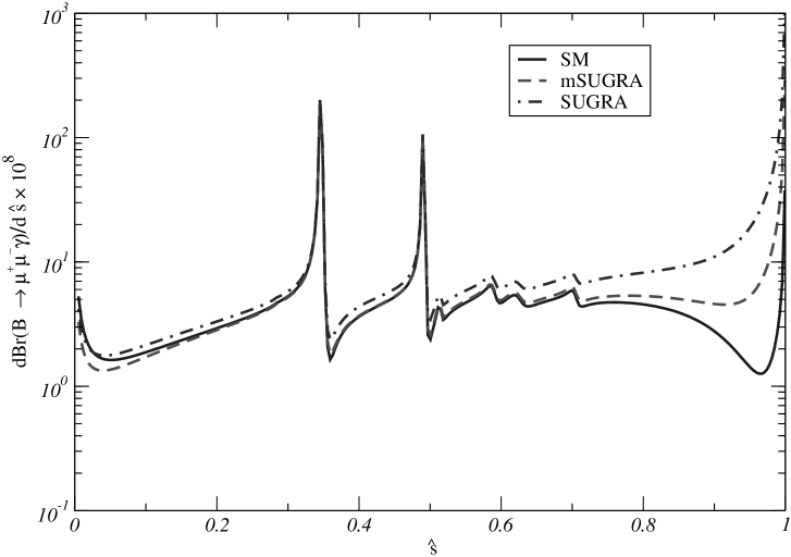
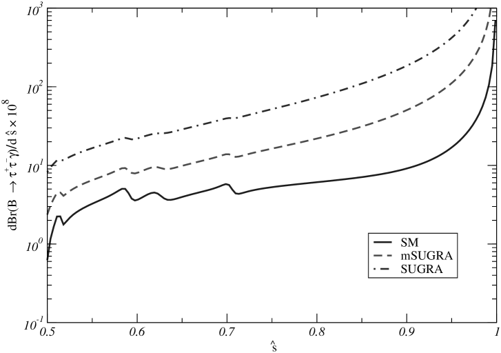
Figure 1: Branching ratios for $B_{s}\to\ell^{+}\ell^{-}\gamma$ with $\ell~{}=~{}\mu$ (above) and $\ell~{}=~{}\tau$ (below). mSUGRA parameters are : $m=200$ GeV, $M=450$ GeV , $A=0$ , $\tan\beta=40$. Additinal parameter for SUGRA (the pseudo-scalar Higgs mass) is taken to be $m_{A}=306$ GeV

Figure(1) shows plots of the differential Braching ratios of $B_{s}\to\ell^{+}\ell^{-}\gamma$ for leptons to be $\mu$ and $\tau$ . The prediction of the Branching ratios for $B_{s}\to\ell^{+}\ell^{-}\gamma$ are :

Table 1: Branching ratios for $B_{s}\to\ell^{+}\ell^{-}\gamma$ ($\ell\ =\mu,\tau$)

Model	Br($B_{s}\to\mu^{+}\mu^{-}\gamma$ )	Br($B_{s}\to\tau^{+}\tau^{-}\gamma$ )
Standard Model	$5.53\times 10^{-8}$	$6.57\times 10^{-8}$
mSUGRA	$6.86\times 10^{-8}$	$3.59\times 10^{-7}$
SUGRA	$1.21\times 10^{-7}$	$1.31\times 10^{-6}$

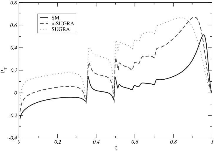
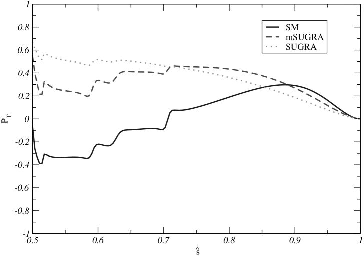
Figure 8: $P_{T}$ for $B_{s}\to\ell^{+}\ell^{-}\gamma$ with $\ell~{}=~{}\mu$ (above) and $\ell~{}=~{}\tau$ (below). mSUGRA parameters are : $m=200$ GeV, $M=450$ GeV , $A=0$ , $\tan\beta=40$. Additinal parameter for SUGRA (the pseudo-scalar Higgs mass) is taken to be $m_{A}=306$ GeV

We have plotted various polarization asymmetries ($P_{L}$ , $P_{T}$ and $P_{N}$ ) in the three models - SM, mSUGRA and SUGRA in Figures(2,5,8) for $B_{s}\to\mu^{+}\mu^{-}\gamma$ and $B_{s}\to\tau^{+}\tau^{-}\gamma$ as a function of $\hat{s}$ (scaled invariant mass of the dilepton pair).

Now we try to analyse the behavior of the polarization asymmetries on the parameters of the models chosen (mSUGRA, and SUGRA). For this analysis we consider the polarization asymmetries at dilepton invariant mass ($\hat{s}$) away from the resonances (the $J/\Psi$) resonances (we choose $\hat{s}=0.68$ for our analysis) . The main focus of the analysis is NHB effects on polarization asymmetries. These effects crucially depend on $tan\beta$ and pseudoscalar Higgs mass ($m_{A}$).

In mSUGRA model the Higgs mass (at electroweak scale) depends crucially on the universal mass of the scalars and $tan\beta$ . To illustrate this crucial behaviour, we have plotted various polarization asymmetries as a function of $tan\beta$ for different values of unified scalar mass ($m$) in Figs. (4, 7, 10) . As can be seen from these figures, $P_{L}$ shows large deviations from the SM values and over a significant portion of the allowed region, even shows a sign flip, provided $tan\beta$ is sufficiently large. Similar behaviour is also there for $P_{T}$ . On the other hand, the predictions for $P_{N}$ don’t differ substantially from SM results but the mSUGRA predictions can change $P_{N}$ by more than 50 % with an appreciable increase in $tan\beta$ .

For SUGRA model we have plotted ( Figs. (4, 7, 10)) the polarization asymmetries as a function of pseudoscalar Higgs mass ($m_{A}$) for various values of $tan\beta$ . In SUGRA we expect more variation of all the polarization asymmetries as compared to their SM values because here we have Higgs mass (pseudo-scalar Higgs mass) as an additional parameter along with $tan\beta$ . As we can see from Figure(4) the variation of $P_{L}$ is more substantial in SUGRA model. In fact for fairly large region of SUGRA parameter space, $P_{L}$ can be opposite in sign as compared to SM case . $P_{T}$ can vary upto five in magnitude when compared with the SM value over the large region of allowed parameter space and for the parameter space we have taken into consideration, the predicted value of $P_{T}$ in SUGRA is opposite in sign to the SM value. Again $P_{N}$ does not show as much deviation as observed for $P_{L}$ and $P_{T}$ but the variation can still be upto an order in certain region.

Summarizing the results of the numerical analysis :

1. From Figures (2,8) it is clear that the longitudinal and transverse polarization asymmetries ($P_{L}$ , $P_{T}$ ) can have substantial deviation from their respective Standard Model values over the whole region of dilepton invariant mass ($\hat{s}$), while Figure(5) indicates deviation for $P_{N}$ from SM values for a limited region of the dilepton invariant mass.

2. As we have pointed out earlier RaiChoudhury:1999qb that for the inclusive process $B\to X_{s}\ell^{+}\ell^{-}$ there is not much deviation from SM results in mSUGRA model. But in radiative dileptonic decay mode, mSUGRA predictions also show large deviations (at least of $P_{L}$ and $P_{T}$ ) from SM results, making it possible to use polarization asymmetries to test mSUGRA model. This is mainly because in the bremmstrahlung part of the matrix elment (${\cal M}_{2}$), the Wilson coefficient $C_{Q_{2}}$ adds on to $C_{10}$ via the combination $(C_{10}+\frac{m_{B_{s}}^{2}}{2m_{\ell}m_{b}}C_{Q_{2}})$ which effectively increases the SM value of $C_{10}$. This doesn’t happen for the process $B\to X_{s}\ell^{+}\ell^{-}$ and this numerically is the reason for the scalar exchanges affecting the $B_{s}\to\ell^{+}\ell^{-}\gamma$ process more than the semi-leptonic one.

3. From Figs. (4, 7, 10) we can see that the polarization asymmetries show a general enhancement with increase in $tan\beta$ and they decrease as the universal scalar mass ($m$) is increased. This is expected because the Higgs boson mass increases with $m$ and thus the contributions of scalar ($C_{Q_{1}}$) and pseudoscalar ($C_{Q_{2}}$) type interactions decrease.

4. As can be seen from the structure of the analytical expressions for various polarization asymmetries ( eqn.(15, 16, 17), they are all different analytic functions of various Wilson coefficients and hence contain independent information. These asymmetries, hence, can also be used for accurate determination of various Wilson coefficients.

In conclusion, we can say that the observation of the polarization asymmetries can be a very useful probe for finding out the new physics effects and testing the structure of the effective Hamiltonian.

Appendix A Input Parameters

$m_{B_{s}}~{}=~{}5.26$ GeV  ,   $m_{c}~{}=~{}1.4$ GeV  ,   $m_{s}~{}=~{}0.2$ GeV

$m_{\mu}~{}=~{}0.106$ GeV  ,  $m_{\tau}~{}=~{}1.77$ GeV  ,  $m_{b}~{}=~{}4.8$ GeV

$m_{W}~{}=~{}80.4$ GeV  ,   $m_{t}~{}=~{}176$ GeV  ,  $|V_{tb}V_{ts}^{*}|~{}=~{}0.045$

$G_{F}~{}=~{}1.17\times 10^{-5}~{}{\rm GeV}^{-2}$  ,  $\alpha~{}=~{}\frac{1}{129}$  ,  $\tau(m_{B_{s}})~{}=~{}1.6\times 10^{-12}$ sec

Appendix B

Definition of A, B, C and D defined in eq(3) are :

$$A = \frac{1}{m_{B_{s}}^{2}}~{}[C_{9}^{eff}G_{1}(p^{2})~{}-~{}2C_{7}^{eff}\frac{m_{b}}{p^{2}}G_{2}(p^{2})],$$

$$B = \frac{1}{m_{B_{s}}^{2}}~{}[C_{9}^{eff}F_{1}(p^{2})~{}-~{}2C_{7}^{eff}\frac{m_{b}}{p^{2}}F_{2}(p^{2})],$$

$$C = \frac{C_{10}}{m_{B_{s}}^{2}}~{}G_{1}(p^{2}),$$

$$D = \frac{C_{10}}{m_{B_{s}}^{2}}~{}F_{1}(p^{2}).$$ (18)

where the form factors definition chosen is Eilam:1995zv

$$\langle\gamma|~{}\bar{s}\gamma_{\mu}(1\pm\gamma_{5})b~{}|B_{s}\rangle = \frac{e}{m_{B_{s}}^{2}}\left\{\varepsilon_{\mu\alpha\beta\sigma}\epsilon_{\alpha}^{*}p_{\beta}q_{\sigma}G_{1}(p^{2})\mp i[(\epsilon_{\mu}^{*}(pq)-(\epsilon^{*}p)q_{\mu})]F_{1}(p^{2})\right\}$$ (19)

$$\langle\gamma|~{}\bar{s}i\sigma_{\mu\nu}p_{\nu}(1\pm\gamma_{5})b~{}|B_{s}\rangle = \frac{e}{m_{B_{s}}^{2}}\left\{\varepsilon_{\mu\alpha\beta\sigma}\epsilon_{\alpha}^{*}p_{\beta}q_{\sigma}G_{2}(p^{2})\pm i[(\epsilon_{\mu}^{*}(pq)-(\epsilon^{*}p)q_{\mu})]F_{2}(p^{2})\right\}$$ (20)

multiplying eq.(19) with $p_{\mu}$ and using equation of motion we can get relation :

$$\langle\gamma|~{}\bar{s}(1\pm\gamma_{5})b~{}|B_{s}\rangle~{}=~{}0$$ (21)

The defination of form factors we are using for numerical analysis is Eilam:1995zv :

$$G_{1}(p^{2})~{}=~{}\frac{1}{1-p^{2}/5.6^{2}}~{}GeV G_{2}(p^{2})~{}=~{}\frac{3.74}{1-p^{2}/40.5}GeV^{2},$$ ,

$$F_{1}(p^{2})~{}=~{}\frac{0.8}{1-p^{2}/6.5^{2}}~{}GeV F_{2}(p^{2})~{}=~{}\frac{0.68}{1-p^{2}/30}~{}GeV^{2}.$$ , (22)

Identities used in calculation of matrix element when photon is radiated from lepton leg :

$$\langle 0|~{}\bar{s}b~{}|B_{s}\rangle = 0$$ (23)

$$\langle 0|~{}\bar{s}\sigma_{\mu\nu}(1+\gamma_{5})b~{}|B_{s}\rangle = 0$$ (24)

$$\langle 0|~{}\bar{s}\gamma_{\mu}\gamma_{5}b~{}|B_{s}\rangle = -~{}if_{B_{s}}P_{B_{s}\mu}$$ (25)

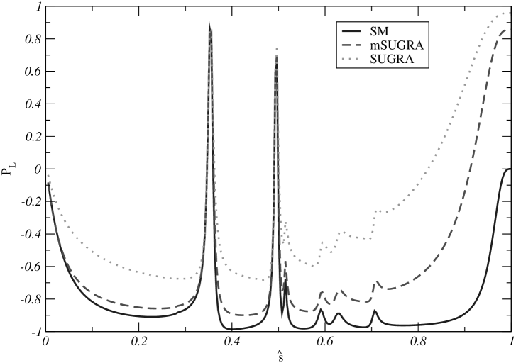
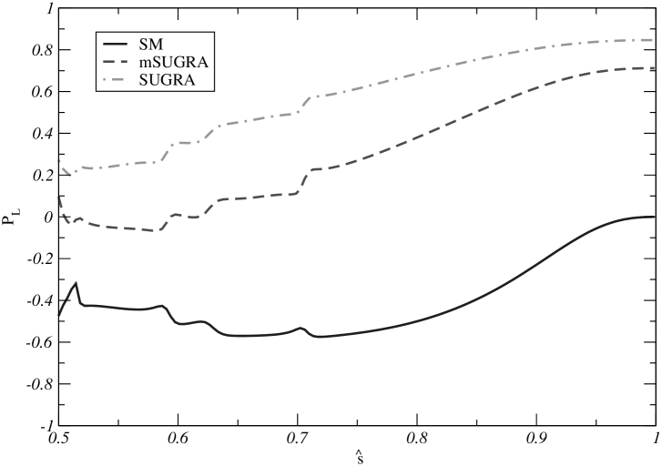
Figure 2: $P_{L}$ for $B_{s}\to\ell^{+}\ell^{-}\gamma$ with $\ell~{}=~{}\mu$ (above) and $\ell~{}=~{}\tau$ (below). mSUGRA parameters are : $m=200$ GeV, $M=450$ GeV , $A=0$ , $\tan\beta=40$. Additinal parameter for SUGRA (the pseudo-scalar Higgs mass) is taken to be $m_{A}=306$ GeV

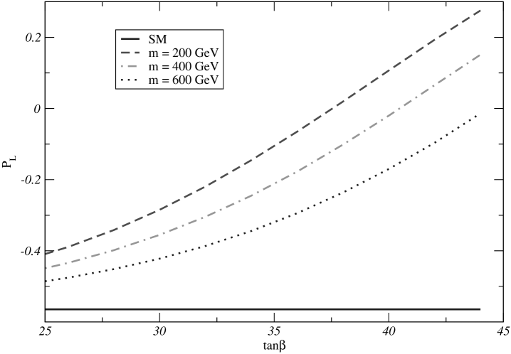
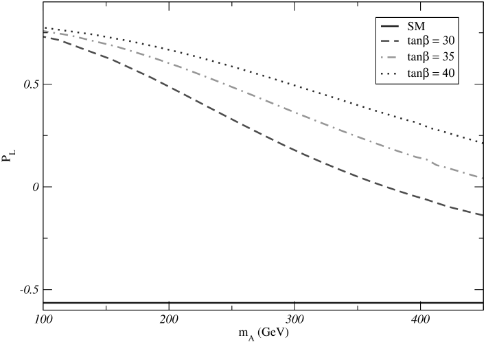
Figure 3: $P_{L}$ vs $tan\beta$ at $\hat{s}=0.68$ for $B_{s}\to\tau^{+}\tau^{-}\gamma$ in mSUGRA model, other parameters are : $M=450$ GeV , $A=0$.

Figure 4: $P_{L}$ vs $m_{A}$ at $\hat{s}=0.68$ for $B_{s}\to\tau^{+}\tau^{-}\gamma$ in SUGRA, other parametes are : $m=200$ GeV , $M=450$ GeV , $A=0$.

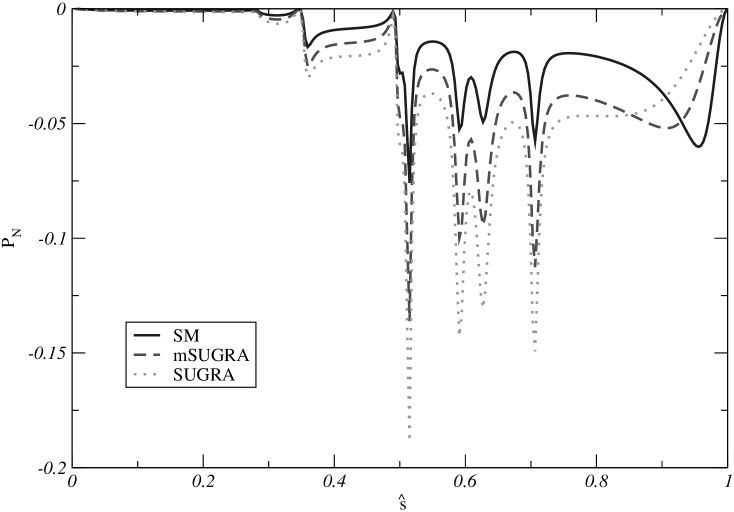
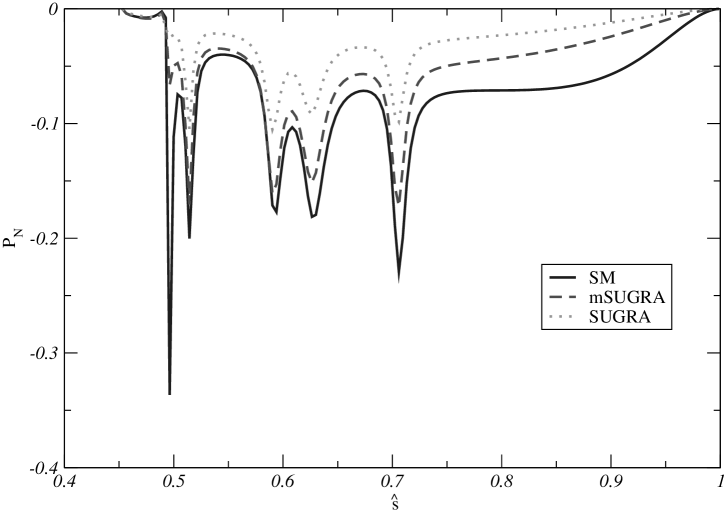
Figure 5: $P_{N}$ for $B_{s}\to\ell^{+}\ell^{-}\gamma$ with $\ell~{}=~{}\mu$ (above) and $\ell~{}=~{}\tau$ (below). mSUGRA parameters are : $m=200$ GeV, $M=450$ GeV , $A=0$ , $\tan\beta=40$. Additinal parameter for SUGRA (the pseudo-scalar Higgs mass) is taken to be $m_{A}=306$ GeV

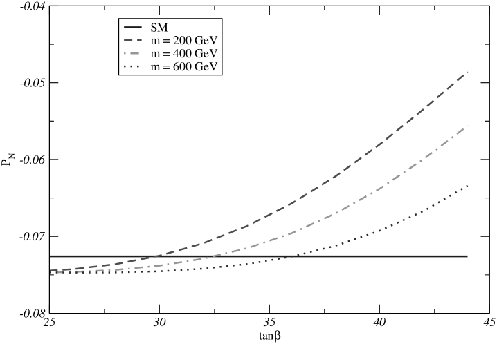
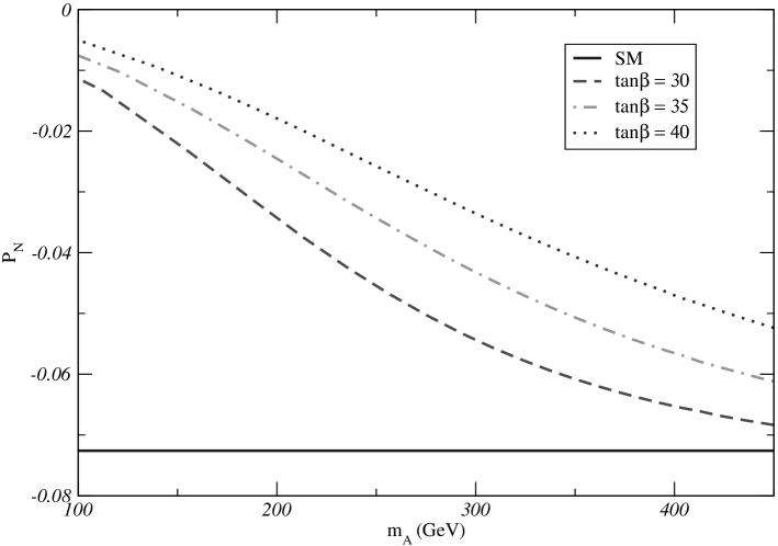
Figure 6: $P_{N}$ vs $tan\beta$ for $B_{s}\to\tau^{+}\tau^{-}\gamma$ at $\hat{s}=0.68$ in mSUGRA , other parameters are : $M=450$ GeV , $A=0$.

Figure 7: $P_{N}$ vs $m_{A}$ at $\hat{s}=0.68$ for $B_{s}\to\tau^{+}\tau^{-}\gamma$ in SUGRA , other parametes are : $m=200$ GeV , $M=450$ GeV , $A=0$.

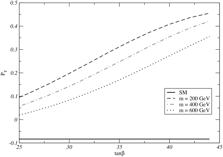
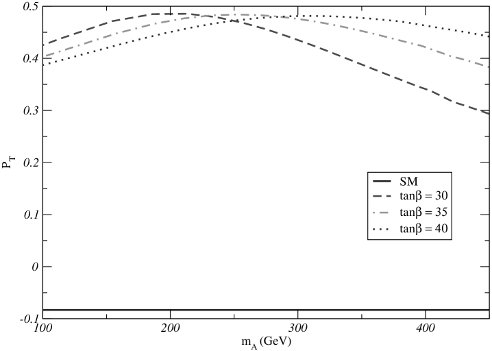
Figure 9: $P_{T}$ vs $tan\beta$ for $B_{s}\to\tau^{+}\tau^{-}\gamma$ at $\hat{s}=0.68$ in mSUGRA , other parameters are : $M=450$ GeV , $A=0$.

Figure 10: $P_{T}$ vs $m_{A}$ for $B_{s}\to\tau^{+}\tau^{-}\gamma$ at $\hat{s}=0.68$ in SUGRA , other parameters are : $m=200$ GeV , $M=450$ GeV , $A=0$.

References

• (1) A. Ali, arXiv:hep-ph/9709507,
G. Buchalla, A. J. Buras and M. E. Lautenbacher, Rev. Mod. Phys.  68, 1125 (1996) [arXiv:hep-ph/9512380].
• (2) E. O. Iltan and G. Turan, Phys.  Rev. D 61, 034010 (2000)[arXiv:hep-ph/9906502] ,
G. Erkol and G. Turan arXiv:hep-ph/0112115
• (3) T. M. Aliev and M. Savci, Phys.  Lett. B 452, 318 (1999)[arXiv:hep-ph/9902208].
• (4) W. Skiba and J. Kalinowski, Nucl.  Phys. B 404, 3 (1993,)
H. E. Logan and U. Nierste, Nucl.  Phys. B 586, 39 (2000)[arXiv:hep-ph/0004139].
• (5) Y. Dai, C. Huang and H. Huang, Phys.  Lett. B 390, 257 (1997)[arXiv:hep-ph/9607389],
• (6) S. R. Choudhury and N. Gaur, Phys.  Lett. B 451, 86 (1999)[arXiv:hep-ph/9810307].
D. A. Demir, K. A. Olive and M. B. Voloshin , arXiv : hep-ph/0204119.
C. Bobeth, T. Ewerth, F. Krüger and J. Urban Phys.  Rev. D 64, 074014 (2001), [arXiv: hep-ph/0104284].
• (7) Z. Xiong and J. M. Yang, Nucl.  Phys. B 628, 193 (2002)[arXiv:hep-ph/0105260].
• (8) C. Huang, W. Liao and Q. Yan, Phys.  Rev. D 59, 011701 (1999)[arXiv:hep-ph/9803460],
• (9) S. Rai Choudhury, A. Gupta and N. Gaur, Phys.  Rev. D 60, 115004 (1999)[arXiv:hep-ph/9902355].
• (10) T. Goto, Y. Okada, Y. Shimizu and M. Tanaka, Phys.  Rev. D 55, 4273 (1997)[arXiv:hep-ph/9609512],
T. Goto, Y. Okada and Y. Shimizu, Phys.  Rev. D 58, 094006 (1998)[arXiv:hep-ph/9804294].
• (11) C. Bobeth, A. J. Buras, F. Kruger and J. Urban, arXiv:hep-ph/0112305.
• (12) P. L. Cho, M. Misiak and D. Wyler, Phys.  Rev. D 54, 3329 (1996)[arXiv:hep-ph/9601360].
• (13) J. L. Hewett and J. D. Wells, Phys.  Rev. D 55, 5549 (1997)[arXiv:hep-ph/9610323].
• (14) M. S. Alam et al. [CLEO Collaboration], Phys.  Rev.  Lett. 74, 2885 (1995,)
R. Ammar et al. [CLEO Collaboration], Phys.  Rev.  Lett. 71, 674 (1993.)
• (15) Y. Grossman, Z. Ligeti and E. Nardi, Phys.  Rev. D 55, 2768 (1997)[arXiv:hep-ph/9607473],
• (16) G. Eilam, C. Lu and D. Zhang, Phys.  Lett. B 391, 461 (1997)[arXiv:hep-ph/9606444],
• (17) T. M. Aliev, A.Özpineci and M. Savci, Phys.  Rev. D 55, 7059 (1997)[arXiv:hep-ph/9611393],
T. M. Aliev, N. K. Pak and M. Savci, Phys.  Lett. B 424, 175 (1998)[arXiv:hep-ph/9710304].
• (18) Y. Dincer and L. M. Sehgal, Phys.  Lett. B 521, 7 (2001)[arXiv:hep-ph/0108144],
C. Q. Geng, C. C. Lih and W. M. Zhang, Phys.  Rev. D 62, 074017 (2000)[arXiv:hep-ph/0007252].
• (19) F. Krüger and L. M. Sehgal, Phys.  Lett. B 380, 199 (1996)[arXiv:hep-ph/9603237],
J. L. Hewett, Phys.  Rev. D 53, 4964 (1996)[arXiv:hep-ph/9506289].
• (20) B. Grinstein, M. J. Savage and M. B. Wise, Nucl.  Phys. B 319, 271 (1989),
A. J. Buras and M. Münz, Phys.  Rev. D 52, 186 (1995)[arXiv:hep-ph/9501281].
• (21) A. Ali, T. Mannel and T. Morozumi, Phys.  Lett. B 273, 505 (1991.)
C. S. Lim, T. Morozumi and A. I. Sanda, Phys.  Lett. B 218, 343 (1989.)
N. G. Deshpande, J. Trampetic and K. Panose, Phys.  Rev. D 39, 1461 (1989.)
P. J. O’Donnell and H. K. Tung, Phys. Rev. D 43, 2067 (1991).
• (22) G. Eilam, I. Halperin and R. R. Mendel, Phys.  Lett. B 361, 137 (1995)[arXiv:hep-ph/9506264].
G. Buchalla and A. J. Buras, Nucl.  Phys. B 400, 225 (1993.)
• (23) B Physics at Tevatron : Run II & Beyond, K.Anikeev et. al. arXiv : hep-ph/0203041 ;
CLEO collaboration, T.E.Coan et. al. Phys.  Rev.  Lett. 84, 5283 (2000)[arXiv : hep-ex/9908022];
ALEPH collaboration, R.Barate et. al. Phys.  Lett. B 429, 169 (1998.)
Refer to caption
Refer to caption