CP-Violation in Kaluza-Klein and Randall-Sundrum Theories

Abstract

The Kaluza-Klein theory and Randall-Sundrum theory are examined comparatively, with focus on the five dimensional (Dirac) fermion and the dimensional reduction to four dimensions. They are treated in the Cartan formalism. The chiral property, localization, anomaly phenomena are examined. The electric and magnetic dipole moment terms naturally appear. The order estimation of the couplings is done. This is a possible origin of the CP-violation.

1 Introduction and Conclusion

If our present research direction of the string and D-brane is right, the unification of various forces should be, effectively at some scale, explained by some higher-dimensional theory. Then it is quite sure that the real world of 4 dimensions should be some approximation of the higher dimensional one. It is realized by the procedure called dimensional reduction. There are two representative and contrastive approaches, that is, the Kaluza-Klein and the Randall-Sundrum theories. In the former case, the reduction is achieved by the compactification of the extra space, while in the latter one it is done by the localization of the configuration along the extra dimension(s). The two approaches look to have both advantages and disadvantages in the phenomenological application. Here we treat them in a comparative way and examine their 4 dimensional(D) reduction properties.

We will present the higher dimensional approach to the CP-violation mechanism. As was stressed by Thirring for the KK model[1], the CP-violation naturally occurs also in the RS model.

2 Fermions in Kaluza-Klein Theory

Let us first review the 5D Kaluza-Klein theory. This serves as the preparation for the same treatment of the Randall-Sundrum theory in the next section. The 5D space-time manifold is described by the 4D coordinates $x^{a}$ ($a=0,1,2,3$) and an extra coordinate $y$. We also use the notation ($X^{m}$)=($x^{a},y$), ($m=0,1,2,3,5$). With the general 5D metric ${\hat{g}}_{mn}$: $ds^{2}={\hat{g}}_{mn}(X)dX^{m}dX^{n}$ , we assume the $S^{1}$ compactification condition for the extra space: ${\hat{g}}_{mn}(x,y)={\hat{g}}_{mn}(x,y+{2\pi}/{\mu})$ , where $\mu^{-1}$ is the radius of the extra space circle. We specify the form of the metric as

$$ds^{2}=g_{ab}(x)dx^{a}dx^{b}+{\rm e}^{\sigma(x)}(dy-fA_{a}(x)dx^{a})^{2}{\quad,}$$ (1)

where $g_{ab}(x),A_{a}(x)$ and $\sigma(x)$ are the 4D metric, the U(1) gauge field and the dilaton field respectively. $f$ is a coupling constant. This specification is based on the following additional assumptions: 1. $y$ is a space coordinate; 2. The geometry is invariant under the U(1) symmetry, $y\rightarrow y+\Lambda(x),\ A_{a}(x)\rightarrow A_{a}(x)+\frac{1}{f}\partial_{a}\Lambda$. We take $\sigma(x)=0$ in (1) for simplicity.

We take the Cartan formalism to compute the geometric quantities[1]. The basis {${\hat{\theta}}^{\mu}$} ($\mu=0,1,2,3,5$ are the local Lorentz (tangent) frame indices) of the cotangent manifold($T_{p}^{*}M$) and the fünf-bein ${\hat{e}}^{\mu}_{~{}m}$ are obtained as

$${\hat{\theta}}^{\alpha}=\theta^{\alpha}=e^{\alpha}_{~{}a}dx^{a},\ {\hat{\theta}}^{5}=dy-fA_{a}dx^{a},A_{\alpha}\equiv e_{\alpha}^{~{}a}A_{a},$$

$$({\hat{e}}^{\mu}_{~{}m})=\left(\begin{array}[]{cc}e^{\alpha}_{~{}a}&0\\ -fA_{a}&1\end{array}\right),\ ({\hat{e}}_{\mu}^{~{}m})=\left(\begin{array}[]{cc}e_{\alpha}^{~{}a}&0\\ fA_{\alpha}&1\end{array}\right),$$ (6)

where $\theta^{\alpha}$ and $e^{\alpha}_{~{}a}$ ($\alpha=0,1,2,3$) are the 4D part of ${\hat{e}}^{\mu}_{~{}m}$ and ${\hat{\theta}}^{\mu}$ respectively. The first Cartan’s structure equation gives the connection 1-form ${\hat{\omega}}^{\mu}_{~{}\nu}$,

$${\hat{\omega}}^{5}_{~{}5}=0,\ {\hat{\omega}}^{5}_{~{}\alpha}=-\frac{f}{2}F_{\alpha\beta}\theta^{\beta},$$

$${\hat{\omega}}^{\alpha}_{~{}\beta}=\omega^{\alpha}_{~{}\beta}-\frac{f}{2}F^{\alpha}_{~{}\beta}{\hat{\theta}}^{5},\ F_{\alpha\beta}\equiv e_{\alpha}^{~{}a}e_{\beta}^{~{}b}F_{ab}{\quad,}$$ (7)

where $\omega^{\alpha}_{~{}\beta}$ is the 4D part.

The 5D Dirac equation is generally given by

$$\left\{\gamma^{\mu}{\hat{e}}_{\mu}^{~{}m}\frac{\partial}{\partial X^{m}}+\frac{1}{8}({\hat{\omega}}^{\sigma})_{\mu\nu}\gamma_{\sigma}[\gamma^{\mu},\gamma^{\nu}]-{\hat{m}}\right\}{\hat{\psi}}=0.$$ (8)

The spin connection above $({\hat{\omega}}^{\sigma})_{\mu\nu}$ is defined by ${\hat{\omega}}^{\mu}_{~{}\nu}=({\hat{\omega}}_{\lambda})^{\mu}_{~{}\nu}{\hat{\theta}}^{\lambda}$. The 5D Dirac matrix $\gamma^{\mu}$ satisfies $\{\gamma^{\mu},\gamma^{\nu}\}=2{\hat{\eta}}^{\mu\nu},{\hat{\eta}}^{\mu\nu}=\mbox{diag}(-1,1,1,1,1)$. For simplicity we switch off the 4D gravity: $e^{\alpha}_{~{}a}\rightarrow\delta^{\alpha}_{a}\ ,\ \omega^{\alpha}_{~{}\beta}\rightarrow 0$. The parameter ${\hat{m}}$ is the 5D fermion mass. In the present case, using (6) and (7), the eq.(8) says

$$\left\{\gamma^{a}(\partial_{a}+fA_{a}\partial_{5})+\gamma^{5}\partial_{5}\right.$$

$$\left.+\frac{f}{16}F_{ab}\gamma^{5}[\gamma^{a},\gamma^{b}]-{\hat{m}}\right\}{\hat{\psi}}=0{\quad.}$$ (9)

We consider the following form of the fermion: ${\hat{\psi}}(x,y)={\rm e}^{i(\phi\gamma_{5}+\mu y)}\psi(x)$ . Here we regard the fermion as a KK-massive mode. The angle parameter $\phi$ is chosen as

$$(i\gamma_{5}\mu+{\hat{m}}){\rm e}^{2i\phi\gamma_{5}}=\sqrt{{{\hat{m}}}^{2}+\mu^{2}}\equiv M,\ \tan 2\phi=-\frac{\mu}{{\hat{m}}}.$$ (10)

Then (9) reduces to

$$\left\{\gamma^{a}(\partial_{a}+ieA_{a})-M+\right.$$

$$\left.\frac{1}{16M}({\hat{m}}\frac{e}{\mu}-ie\gamma_{5})F_{ab}\gamma^{5}[\gamma^{a},\gamma^{b}]\right\}\psi=0{\quad,}$$ (11)

where $e\equiv f\mu$ is the electric coupling constant. We notice, in this expression, the electric and magnetic moments appear.

$$\frac{1}{16}\frac{{\hat{m}}}{M\mu}eF_{ab}{\bar{\psi}}\gamma^{5}[\gamma^{a},\gamma^{b}]\psi,\ -\frac{i}{16}\frac{1}{M}eF_{ab}{\bar{\psi}}[\gamma^{a},\gamma^{b}]\psi.$$ (12)

The first term violate the CP symmetry. Note that the second term usually appear, in the 4D QED, as the quantum effects.

Let us do the order estimation. From the reduction of $\int\sqrt{-{\hat{g}}}{\cal L}^{grav}=\frac{1}{G_{5}}\int d^{5}X\sqrt{-{\hat{g}}}{\hat{R}}$,

$$\frac{1}{G_{5}}\frac{2\pi}{\mu}\int d^{4}x\sqrt{-g}(R-\frac{f^{2}}{4}F^{\alpha\beta}F_{\alpha\beta}+\cdots),$$ (13)

we know ${G_{5}\mu}\sim{G},\ {f^{2}}/{G_{5}\mu}\sim 1$ , where $G$ is the gravitational constant. This gives $f\sim\sqrt{G}=10^{-19}\mbox{GeV}^{-1}$. On the other hand, we know $e=\mu f\sim 10^{-1}$. Hence we obtain $\mu\sim 10^{-1}f^{-1}\sim 10^{18}\mbox{GeV}$. Assuming ${\hat{m}}\sim\mu$, we can estimate the electric and magnetic couplings as

$$\frac{{\hat{m}}}{M\mu}e\sim\frac{e}{M}\sim 10^{-19}\mbox{GeV}^{-1}\sim 10^{-32}\mbox{e cm}{\quad,}$$ (14)

which is far below the experimental upper bound of the neutron electric dipole moment $6.3\times 10^{-26}$e cm.

3 Fermions in Randall-Sundrum Geometry

We consider the following 5D space-time geometry[2].

$$ds^{2}={\rm e}^{-2\sigma(y)}\eta_{ab}dx^{a}dx^{b}+dy^{2}={\hat{g}}_{mn}dX^{m}dX^{n},$$

$$-\infty<y<+\infty\ ,\ -\infty<x^{a}<+\infty,$$ (15)

where $\sigma(y)$ is regarded as a scale factor field. $(\eta_{ab})=\mbox{diag}(-1,1,1,1)$. When the geometry is AdS₅, $\sigma(y)=c|y|,c>0$. Such a situation, in the present case, occurs in the asymptotic region of the extra space $y\rightarrow\pm\infty$. The 1-form ${\hat{\theta}}^{\mu}$, the fünf-bein ${\hat{e}}^{\mu}_{~{}m}$ and the connection 1-form ${\hat{\omega}}^{\mu}_{~{}\nu}$ are given by

$${\hat{\theta}}^{\alpha}={\rm e}^{-\sigma}\eta^{\alpha}_{~{}a}dx^{a}{\quad,}\quad{\hat{\theta}}^{5}=dy{\quad,}$$

$$({\hat{e}}^{\mu}_{~{}m})=\left(\begin{array}[]{cc}e^{-\sigma}\eta^{\alpha}_{~{}a}&0\\ 0&1\end{array}\right),\ ({\hat{e}}_{\mu}^{~{}m})=\left(\begin{array}[]{cc}e^{\sigma}\eta_{\alpha}^{~{}a}&0\\ 0&1\end{array}\right),$$ (20)

$${\hat{\omega}}^{5}_{~{}5}=0{\quad,}\quad{\hat{\omega}}^{\alpha}_{~{}5}=-{\hat{\omega}}_{5}^{~{}\alpha}=-\sigma^{\prime}\theta^{\alpha}{\quad,}$$

$${\hat{\omega}}^{5}_{~{}\alpha}=-{\hat{\omega}}_{\alpha}^{~{}5}=\sigma^{\prime}\theta_{\alpha}{\quad,}\quad{\hat{\omega}}^{\alpha}_{~{}\beta}=0{\quad,}$$ (21)

where $\sigma^{\prime}=\frac{d\sigma}{dy}$.

As the fermion model, the (5D) Dirac theory (8), $\sqrt{-{\hat{g}}}{\cal L}^{Dirac}$, is not accepted physically because the fermion configuration does not localize (around $y=0$) in the extra space. Nature requires the Yukawa interaction between the 5D fermion and the 5D Higgs[3].

Hence we examine the fermion behavior under the Yukawa coupling with the Higgs scalar: $\sqrt{-{\hat{g}}}{\cal L}=\sqrt{-{\hat{g}}}({\cal L}^{Dirac}+{\cal L}^{Y}),\ {\cal L}^{Y}=ig_{Y}{\bar{\hat{\psi}}}{\hat{\psi}}\Phi,$ where $\Phi$ is the 5D(bulk) Higgs scalar field and $g_{Y}$ is the Yukawa coupling. This reduces to

$$i{\rm e}^{\sigma}\{\gamma^{a}\partial_{a}+2{\rm e}^{-\sigma}(\sigma^{\prime}-{\frac{1}{2}}\partial_{y})\gamma_{5}-g_{Y}{\rm e}^{-\sigma}\Phi\}{\hat{\psi}}=0.$$ (22)

A solution of the right chirality zero mode: ${\hat{\psi}}(x,y)=\psi^{0}_{R}(x)\eta(y),\ \gamma_{5}\psi^{0}_{R}=+\psi^{0}_{R},\ \gamma^{a}\partial_{a}\psi^{0}_{R}=0$ , is obtained by

$$\partial_{y}\eta=(2\sigma^{\prime}-g_{Y}\Phi(y))\eta{\quad.}$$ (23)

In the far region, the solution behaves as $\eta(y)=\mbox{const}\times{\rm e}^{-(g_{Y}{v_{0}}-2\omega)|y|}$ , which shows the exponentially damping for the large yukawa coupling $g_{Y}>2\omega/{v_{0}}$. ($\omega$ and ${v_{0}}$ is the asymptotic values of $\sigma^{\prime}(y)$ and $\Phi(y)$[4]. ) This is called massless chiral fermion localization. In the near region, $\eta(y)=\mbox{const}\times{\rm e}^{-\frac{k}{2}(g_{Y}{v_{0}}-2\omega)y^{2}}$ , which shows the Gaussian damping. ($1/k$ is the thickness parameter of the wall. )

Now we analyze the 5D QED, ${\cal L}^{QED}=-e{\bar{\hat{\psi}}}\gamma^{\mu}{\hat{e}}_{\mu}^{~{}m}{\hat{\psi}}A_{m}$, with the Yukawa interaction in RS geometry: $\sqrt{-{\hat{g}}}({\cal L}^{Dirac}+{\cal L}^{EM}+{\cal L}^{QED}+{\cal L}^{Y}),{\cal L}^{EM}=-\frac{1}{4}{\hat{g}}^{mn}{\hat{g}}^{kl}F_{mk}F_{nl}$ . We assume, as in the previous paragraph, ${\hat{g}}^{mn}$ and $\Phi$ are the brane background obtained from the gravitational and Higgs systems: $\sqrt{-{\hat{g}}}({\cal L}^{grav}+{\cal L}^{S})$.

Let us examine the bulk quantum effect. It induces the 5D effective action $S_{eff}$ which reduces to the 4D action in the thin wall limit. From the diagram of Fig.1(left), we expect

$$\frac{\delta S^{(1)}_{eff}}{\delta A^{\mu}(X)}\equiv<J_{\mu}>\sim e^{2}g_{Y}\epsilon_{{\mu\nu}{\lambda\sigma}\tau}\Phi F^{\nu\lambda}F^{\sigma\tau}{\quad.}$$ (24)

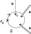
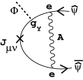
Figure 1: The left diagram induces the effective action $S^{(1)}_{eff}$, while the right one induces $S^{(2)}_{eff}$.

Then the effective action is integrated as

$$S^{(1)}_{eff}\sim e^{2}g_{Y}\int d^{5}X\epsilon_{{\mu\nu}{\lambda\sigma}\tau}\Phi A^{\mu}F^{\nu\lambda}F^{\sigma\tau}{\quad.}$$ (25)

In the thin wall limit we may approximate as $\Phi=\Phi(y)\sim{v_{0}}\epsilon(y)$ where $\epsilon(y)$ is the step function. Under the U(1) gauge transformation $\delta A^{\mu}=\partial^{\mu}\Lambda$, $S^{(1)}_{eff}$ changes as

$$\delta_{\Lambda}S^{(1)}_{eff}\sim e^{2}g_{Y}{v_{0}}\int d^{5}X\epsilon_{{\mu\nu}{\lambda\sigma}\tau}\epsilon(y)\partial^{\mu}\Lambda F^{\nu\lambda}F^{\sigma\tau}$$

$$=-e^{2}g_{Y}{v_{0}}\int d^{4}x\Lambda(x)F^{{\alpha\beta}}{\tilde{F}}_{{\alpha\beta}}{\quad,}$$ (26)

where ${\tilde{F}}_{{\alpha\beta}}\equiv\epsilon_{{\alpha\beta}\gamma\delta}F^{\gamma\delta}$. In the above we assume that the boundary term vanishes. Callan and Harvey interpreted this result as the ”anomaly flow” between the boundary (our 4D world) and the bulk[5].

Through the analysis of the induced action in the bulk, we can see the ”dual” aspect of the 4D QED.

Another interesting bulk quantum effect is given by Fig.1(right). The induced effective action $S^{(2)}_{eff}$ is expected to satisfy

$$\frac{\delta S^{(2)}_{eff}}{\delta F^{\mu\nu}}\equiv<J_{\mu\nu}>\sim e^{2}g_{Y}\epsilon_{{\mu\nu}{\lambda\sigma}\tau}\partial^{\lambda}\Phi{\bar{\hat{\psi}}}\Sigma^{\sigma\tau}{\hat{\psi}}{\quad.}$$ (27)

Then $S^{(2)}_{eff}$ is obtained as, in the thin wall limit,

$$S^{(2)}_{eff}\sim e^{2}g_{Y}\epsilon_{{\mu\nu}{\lambda\sigma}\tau}\int d^{5}X\partial^{\lambda}\Phi F^{\mu\nu}{\bar{\hat{\psi}}}\Sigma^{\sigma\tau}{\hat{\psi}}$$

$$=e^{2}g_{Y}{v_{0}}\epsilon_{{\alpha\beta}{\gamma\delta}}\int d^{4}xF^{\alpha\beta}{\bar{\psi}}\sigma^{{\gamma\delta}}\psi{\quad.}$$ (28)

This term is the ”dual” of the magnetic moment term of (12). It is a CP-violating term. The coupling depends on the vacuum expectation value of $\Phi$.

References

• [1] W. Thirring, Acta Physica Austriaca, Suppl.IX, 256-271(1972), Springer-Verlag, ”Fivedimensional Theories and CP-Violation”
• [2] L.Randall and R.Sundrum, Phys.Rev.Lett.83(1999)3370,4690
• [3] B.Bajc and G.Gabadadze, Phys.Lett.B474(2000)282
• [4] S.Ichinose,Class.Quant.Grav.18(2001)421,5239
• [5] C.G.Callan and J.A.Harvey,Nucl.Phys.B250(1985)427