Lattice QCD with Dynamical Quarks from the UKQCD Collaboration

Abstract

A brief overview of the lattice technique of studying QCD is presented. Recent results from the UKQCD Collaboration’s simulations with dynamical quarks are then presented. In this work, the calculations are all at a fixed lattice spacing and volume, but varying sea quark mass from infinite (corresponding to the quenched simulation) down to roughly that of the strange quark mass. The main aim of this work is to uncover dynamical quark effects from these “matched” ensembles.

1 Introduction

In lattice QCD, the quark degrees of freedom are defined on the sites of the 4-dimensional lattice, and the gluonic degrees of freedom are defined on the links between the lattice vertices. This enables a lattice version of the theory to be defined which maintains as many of the symmetries of the continuum theory as possible. (For a reviews of lattice QCD see [1].)

As in other theoretical field theory techniques, typical quantities of interest can then be expressed as $n$-point functions, $G_{n}(t)$, of hadronic operators. Quantities of physical interest, such as hadronic masses, can be extracted from calculations of the 2-point function $G_{2}(t)$ as follows. It can be shown that (in Euclidean space-time),

$$G_{2}(t)=\sum_{i}Z_{i}e^{-M_{i}t}\rightarrow Z_{0}e^{-M_{0}t}\;\;\;\mbox{as }t\rightarrow\infty.$$ (1)

The sum is over all states $|i>$ with the same quantum numbers as the operators which define the 2-point function, $G_{2}(t)$. Hence the ground state mass of a hadron, $M_{0}$, can be extracted simply by fitting $G_{2}(t)$ to an exponential at sufficiently large times $t$.

This is not the end of the story though because $M_{0}$ (and any other quantity extracted from a lattice calculation) is a function of the input parameters of the simulation. These are the coupling strength $g_{0}$, the quark mass $m$ and the volume $L^{3}$. Ideally what is required is the continuum limit, $a\rightarrow 0$ of $M_{0}$ ($a$ is the lattice spacing) which corresponds to $g_{0}\rightarrow 0$ (since QCD is asymptotically free). However, as has been found by several groups (e.g. [2, 3]), the (dynamical or sea) quark mass $m^{sea}$ also has impact on the lattice spacing $a$, i.e. $a=f(g_{0},m^{sea})$.

Another issue regarding lattice QCD is the error which is introduced in the discretisation of the continuum theory. In the conventional approach, the lattice action reproduces the continuum action only up to terms of ${\cal O}(a)$. Over the last several years, lattice groups, including UKQCD, have been using so-called improved versions of the lattice action which have lattice errors of ${\cal O}(a^{2})$. While this is an obvious improvement over conventional lattice actions, it does not preclude lattice results being contaminated with lattice artefacts, all-be-it at the ${\cal O}(a^{2})$ level.

In order to establish a clean signal it is imperative to fix $a=$ const for two reasons: (i) since the lattice calculation leaves the answer correct to ${\cal O}(a^{2})$, to keep this error constant, $a$ must be fixed; (ii) in order to maintain fixed finite-size effects, $a$ must be fixed (simply because the lattice size $L=Na$ where $N$ is the number of lattice sites along a side). Since $a=f(g_{0},m^{sea})$ (see above) the requirement that $a=$ const defines a “matched” trajectory in the $(g_{0},m^{sea})$ plane.

The UKQCD Collaboration has embarked upon a study of dynamical quark effects in QCD lattice simulations by simulating along a matched trajectory. This paper presents an overview of this work. See [4] for a full description.

2 Simulation Details

The standard Wilson gauge action was used together with the Clover ${\cal O}(a)$-improved fermion action. The coefficient, $c_{SW}$, used in the Clover term was non-perturbatively determined by the Alpha Collaboration [5].

A range of $(\beta,\mbox{$\kappa^{\rm sea}$})$ values were chosen in order to maintain a constant value of the lattice spacing ($\beta=6/g_{0}^{2}$). This used the technology of [6]. The parameter values for the simulations are displayed in Table 1. The lattice volume used was $16^{3}\times 32$ throughout.

Table 1 lists also the lattice spacing obtained from the Sommer scale, $r_{0}$ [7]. The first error listed is statistical, and the second (shown as ${\scriptstyle{}^{+{x}}_{-{y}}}$) is the systematic error from variations in the fit used for the static quark potential. The central values quoted were obtained using all potential data satisfying $\sqrt{2}\leq\mbox{\boldmath${r}$}\leq 8$. It can be seen that the last four simulations listed (i.e. those at $\mbox{$\kappa^{\rm sea}$}=0.1350,0.1345,0.1340$ and $0$) are matched to within errors, with the $\mbox{$\kappa^{\rm sea}$}=0$ simulation corresponding to a quenched run.

The simulations at $\mbox{$\kappa^{\rm sea}$}=0.1355$ and $0.13565$ were performed in order to study lighter sea quark masses and do not lie on the above matched trajectory.

Full details of autocorrelation times and other algorithmic issues can be found in [4].

Table 1: Lattice parameters together with measurements of $a$ and quark masses.

$\beta$	$\kappa^{\rm sea}$	$c_{SW}$	#conf.	$a_{r_{0}}$ [Fm]	$a_{J}$ [Fm]	$M_{PS}^{unitary}/M_{V}^{unitary}$
5.20	0.13565	2.0171	244	0.0941(8)${\scriptstyle{}^{+{13}}_{-{0}}}$	-	-
5.20	0.1355	2.0171	208	0.0972(8)${\scriptstyle{}^{+{7}}_{-{0}}}$	0.110${\scriptstyle{}^{+{4}}_{-{3}}}$	0.578${\scriptstyle{}^{+{13}}_{-{19}}}$
5.20	0.1350	2.0171	150	0.1031(09)${\scriptstyle{}^{+{20}}_{-{1}}}$	0.115${\scriptstyle{}^{+{3}}_{-{3}}}$	0.700${\scriptstyle{}^{+{12}}_{-{10}}}$
5.26	0.1345	1.9497	101	0.1041(12)${\scriptstyle{}^{+{11}}_{-{10}}}$	0.118${\scriptstyle{}^{+{2}}_{-{2}}}$	0.783${\scriptstyle{}^{+{5}}_{-{5}}}$
5.29	0.1340	1.9192	101	0.1018(10)${\scriptstyle{}^{+{20}}_{-{7}}}$	0.116${\scriptstyle{}^{+{3}}_{-{4}}}$	0.835${\scriptstyle{}^{+{7}}_{-{7}}}$
5.93	0	1.82	623	0.1040(03)${\scriptstyle{}^{+{4}}_{-{0}}}$	0.1186${\scriptstyle{}^{+{17}}_{-{15}}}$	1

3 The static potential

The static quark potential was determined for all our ensembles using the method originally proposed in [8] and using a variational basis of “fuzzed” links [9].

Figure 1: The static QCD potential expressed in units of $r_{0}$. The dashed curve is a string model described in the text.

Figure 2: The difference between the static QCD potential expressed in physical units and the prediction of the string model described in the text. For clarity, only data from the matched ensembles are shown.

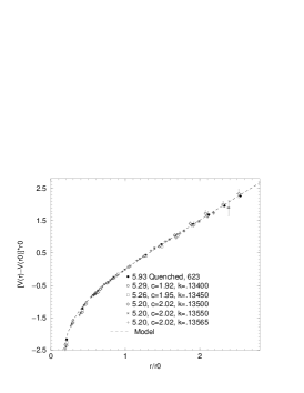
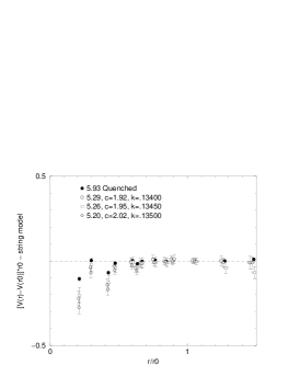
Figure 1 plots the static potential in units of $r_{0}$. The zero of the potential has been set at $r=r_{0}$. The data are well described by the universal bosonic string model potential [10] which predicts

$$\big{[}V(r)-V(r_{0})\big{]}r_{0} = (1.65-e)\left(\frac{r}{r_{0}}-1\right)$$ (2)

$$- e\left(\frac{r_{0}}{r}-1\right)\,.$$

Of course, the fact that the scaled potential measurements all have the same value and slope at $r=r_{0}$ simply reflects the definition of $r_{0}$. Figure 2 shows the deviations from this model potential for the matched ensembles. Here $e=\pi/12$ [10].

Overall there is no discernable difference between the ensembles at distance $r\approx r_{0}$. Furthermore, the data follow the string model very well. However, at shorter distances, $r<0.5r_{0}$, there is a deviation from the string model, and a variation amongst the ensembles. This seems to be systematic in the sea quark mass – the deviation from the string model increases as $m^{sea}$ decreases. In fact, careful correlated fits of the potential show that the parameter $e$ in Eq.(2) increases by 18${\scriptstyle{}^{+{13}}_{-{10}}}$% in going from the quenched to $\mbox{$\kappa^{\rm sea}$}=.13500$ data. We note that the ensembles in Figure 2 are matched, and therefore we can exclude lattice systematics from the effects that we have observed. (Similar findings in the case of two flavours of Wilson fermions have been reported by the SESAM-T$\chi$L collaboration [11] where an increase of $16-33\%$ was found.) Finally we note that there is no evidence of string breaking in our static quark potential. However the distance scales covered $r\;\raisebox{-2.15277pt}{\hbox to0.0pt{$\sim$\hss}}\raisebox{2.15277pt}{$<$}\;1.3fm$ is not large.

4 Hadronic Spectrum

In this section one of our main aims will be to uncover unquenching effects in the light hadron spectrum. Because we have a matched data set, any variation amongst our ensembles can be attributed to unquenching effects. However, the task of identifying variations is likely to be hard for those quantities which are primarily sensitive to physics at the same scale as that used to define the matching trajectory in the $(\beta,\mbox{$\kappa^{\rm sea}$})$ parameter space ($r_{0}$ in this case). This is expected to be the case for the hadron spectrum considered here where the quark masses are still relatively heavy.

Two-point hadronic correlation functions were produced for each of the ensembles using interpolating operators for pseudoscalar, vector, nucleon and delta channels as described in [12]. Mesonic correlators were constructed using both degenerate and non-degenerate valence quarks, whereas only degenerate valence quarks were used for the baryonic correlators. Full details of the fitting procedure can be found in [4].

4.1 The J parameter

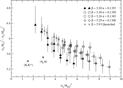
In Figures 3 and 4 the vector meson masses and hyperfine splittings are plotted against the corresponding pseudoscalar masses for all the datasets. It is difficult to identify an unquenching signal from these plots - the data seem to overlay each other. Note that in [3], it was reported that there was a tendency for the vector mass to increase as the sea quark mass decreases (for fixed pseudoscalar mass). The observations for the present matched dataset imply that this may have been due to either an ${\cal O}(a)$ effect (since the dataset in [3] was not fully improved at this level) or a finite volume effect. The conclusion therefore is that it is important to run at a fixed $a$ in order to disentangle unquenching effects from lattice artifacts or finite volume effects.

Figure 3: Vector mass plotted against pseudoscalar mass squared in units of $r_{0}$, together with the experimental data points.

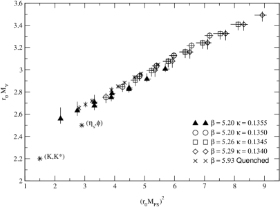
A possible explanation for the lack of convincing unquenching effects in our meson spectrum is the following. Our matched ensembles are defined to have a common $r_{0}$ value, so any physical quantity that is sensitive to this distance scale (and the static quark potential itself) will also, by definition, be matched. Our mesons, because they are composed of relatively heavy quarks, are examples of such quantities, and this is a possible reason why there is no significant evidence of unquenching effects in the meson spectrum.

A further point regarding hyperfine splitting in Figure 4 is that the lattice data for the matched ensembles tends to flatten as the sea quark mass decreases. (The quenched data has a distinctly negative slope, whereas the $\mbox{$\kappa^{\rm sea}$}=0.1350$ data is flat.) Thus the lattice data is tending towards the same behaviour as the experimental data which lies on a line with positive slope (independent of the value used for $r_{0}$). This behaviour is apparently spoiled by the unmatched run with $\mbox{$\kappa^{\rm sea}$}=0.1355$ (see Figure 4) which has a clear negative slope. However, the $\mbox{$\kappa^{\rm sea}$}=0.1355$ data does not satisfy the finite volume bound of [3], and therefore we can attribute the trend in this data to a lattice artefact.

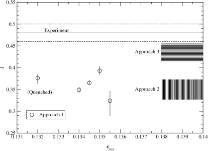
We now study the $J$-parameter defined as [13]

$$J=M_{V}\frac{dM_{V}}{dM_{PS}^{2}}\bigg{|}_{K,K^{\ast}}.$$ (3)

Figure 4: The hyperfine splitting.

In the context of dynamical fermion simulations, this parameter can be calculated in two ways. The first is to define a partially quenched $J$ for each value of the sea quark mass. In this case, the derivative in (3) is with respect to variations in the valence quark mass (with the sea quark mass fixed). The second approach is to define $J$ along what we will term the ‘unitary’ trajectory, i.e. along $\mbox{$\kappa^{\rm sea}$}=\mbox{$\kappa^{\rm val}$}$. In Table 2, the results from both methods are given. These values of $J$ are around 25% lower than the experimental value $J_{expt}=0.48(2)$.

	$\beta$	$\kappa^{\rm sea}$	$J$
First Approach
	5.2000	0.1355	0.32${\scriptstyle{}^{+{2}}_{-{4}}}$
	5.2000	0.1350	0.393${\scriptstyle{}^{+{10}}_{-{9}}}$
	5.2600	0.1345	0.365${\scriptstyle{}^{+{6}}_{-{6}}}$
	5.2900	0.1340	0.349${\scriptstyle{}^{+{7}}_{-{8}}}$
	5.9300	0.0000	0.376${\scriptstyle{}^{+{9}}_{-{12}}}$
Second Approach
	-	-	0.35${\scriptstyle{}^{+{2}}_{-{2}}}$
Third Approach
	-	-	0.43${\scriptstyle{}^{+{2}}_{-{2}}}$

Table 2: $J$ values from the various approaches as described in the text.

Finally we note that the physical value of $J$ (i.e. that which most closely follows the procedure used to determine the experimental value of $J_{expt}=0.48(2)$), should be obtained from extrapolating the results from the first approach to the physical sea quark masses. We call this the third approach. In order to perform this extrapolation, we extrapolate the three matched dynamical $J$ values obtained from the first approach linearly in $(M_{PS}^{\rm unitary})^{2}$ to $(M_{PS}^{\rm unitary})^{2}=0$. $M_{PS}^{\rm unitary}$ is the pseudoscalar meson mass at the unitary point. The value for $J$ from the third approach is presented in Table 2 and we note that it is approaching the experimental value for $J$.

The results from all three approaches are plotted in Figure 5, together with the experimental result. There is some promising evidence that the lattice estimate of $J$ increases towards the experimental point as the sea quark mass decreases (see the $J$ value from approaches 1 and 3).

Figure 5: $J$ versus $\kappa^{sea}$ using the approaches as described in the text. Note that the quenched data points have been plotted at $\mbox{$\kappa^{\rm sea}$}=0.132$ for convenience. Approaches 2 & 3 are obtained after a chiral extrapolation and are shown as banded regions. The experimental value $J=0.48(2)$ is also shown.

Recently there has been a proposed ansatz for the functional form of $M_{V}$ as a function of $M_{PS}^{2}$ [14]. Although this ansatz would be interesting to pursue, all our data have $M_{PS}/M_{V}\;\raisebox{-2.15277pt}{\hbox to0.0pt{$\sim$\hss}}\raisebox{2.15277pt}{$>$}\;0.6$, and for this region, the ansatz of [14] is linear to high precision. Therefore we have chosen to interpolate our data with a simple linear function and await more chiral data before using the ansatz of [14].

4.2 Lattice spacing

This subsection presents a determination of $a$ from the meson spectrum which complements that from $r_{0}$.

A common method of determining $a$ from the meson spectrum uses the $\rho$ mass. However, this requires the chiral extrapolation of the vector meson mass down to (almost) the chiral limit which, as was discussed in the previous subsection, may be problematic. An alternative method of extracting the lattice spacing using the vector meson mass at the simulated data points (i.e. without any chiral extrapolation) was given in [15]. Using this method, we obtain the lattice spacing values as shown in Table 1 labelled $a_{J}$. Note that these are in general 10-15% larger than the values from Section 3 where the lattice spacing was determined from $r_{0}$. A possible explanation for this discrepancy is that the potential and mesonic spectrum are contaminated with different ${\cal O}(a^{2})$ errors (or that the value $r_{0}=0.49$ fm is 10-15% too small!).

In order to investigate unquenching effects in the meson spectrum, we define the quantity

$$\delta_{i,j}(\beta,m^{sea})=1-\frac{a_{i}(\beta,m^{sea})}{a_{j}(\beta,m^{sea})},$$ (4)

where $a_{i}$ is the lattice spacing determined from the physical quantity $i=\{M_{\rho},M_{K},f_{\pi}\ldots\}$. Note that when $\delta_{i,j}=0$, the lattice prediction of $M_{i}$ with scale taken from $M_{j}$ agrees with experiment. Thus $\delta$ is a good parameter to study unquenching effects. We expect that $\delta_{i,j}(\beta,m^{sea})={\cal O}(a^{2})$ since we are working with a non-perturbatively improved clover action.

In Figure 6, $\delta_{i,j}$ is plotted against $(aM_{PS}^{\rm unitary})^{-2}$ for the matched datasets. In this plot we have fixed $j=r_{0}$ and the various physical quantities $i$ are $\sqrt{\sigma}$ (the string tension) and the hadronic mass pairs $(M_{K}*,M_{K})$ & $(M_{\rho},M_{\pi})$. The method used to determine the scale $a_{i}$ from these mass pairs is that of [15]. It is worth noting that the experimental point on this same plot would occur at an $x-$co-ordinate (depressingly) of $(aM_{PS}^{\rm unitary})^{-2}=(aM_{\pi})^{-2}\approx 200$.

Figure 6: $\delta_{i}$ as a function of $1/(aM^{unitary}_{PS})^{2}$ for $i=\sqrt{\sigma}$ and the mass pairs $(M_{K}*,M_{K})$ & $(M_{\rho},M_{\pi})$. $\delta_{i}$ is defined in eq.(4) with $j=r_{0}$.

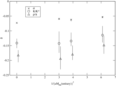
Figure 6 does not show signs of unquenching for quantities involving the hadronic spectrum i.e. the mass pairs $(M_{K}*,M_{K})$ & $(M_{\rho},M_{\pi})$. However, there is evidence of unquenching effects when comparing the scale from $r_{0}$ with that from $\sqrt{\sigma}$ since the quenched value of $\delta_{\sqrt{\sigma}}$ is distinct from the dynamical values.

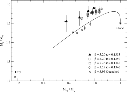
4.3 Edinburgh Plot

In Table 1 the ratios $M_{PS}/M_{V}$ are displayed for the unitary case $\mbox{$\kappa^{\rm sea}$}=\mbox{$\kappa^{\rm val}$}$. As can be seen the simulated data is a long way from the experimental value $M_{\pi}/M_{\rho}=0.18$. Figure 7 shows the ‘Edinburgh plot’ ($M_{N}/M_{V}$ v.s. $M_{PS}/M_{V}$) for all the data sets. There is no significant variation within the dynamical data as the sea quark mass is changed, but the dynamical data does tend to lie above the (matched) quenched data. This latter feature may be indicative of finite volume effects since these are expected to be larger in full QCD compared to the quenched case [16].

Figure 7: The Edinburgh plot for all the data sets. All degenerate $\kappa^{\rm val}$ correlators have been included. The phenomenological curve (from [17]) has been included as a guide to the eye.

5 Chiral Extrapolations

In [4] we used 3 approaches to perform the chiral extrapolations of hadron masses: “Pseudo-Quenched”; “Unitary Trajectory”; and a “Combined Chiral Fit”. In this publication we will refer only to the last approach. We take

$$\hat{M}(\mbox{$\kappa^{\rm sea}$};\mbox{$\kappa^{\rm val}$})$$

$$\;\;\;\;\;\;\;\;\;\;\;\;=A(\mbox{$\kappa^{\rm sea}$})+B(\mbox{$\kappa^{\rm sea}$})\hat{M}_{PS}(\mbox{$\kappa^{\rm sea}$};\mbox{$\kappa^{\rm val}$})^{2}$$

$$\;\;\;\;\;\;\;\;\;\;\;\;=A_{0}+A_{1}\hat{M}_{PS}(\mbox{$\kappa^{\rm sea}$};\mbox{$\kappa^{\rm sea}$})^{-2}$$

$$+\left[B_{0}+B_{1}\hat{M}_{PS}(\mbox{$\kappa^{\rm sea}$};\mbox{$\kappa^{\rm sea}$})^{-2}\right]\hat{M}_{PS}(\mbox{$\kappa^{\rm sea}$};\mbox{$\kappa^{\rm val}$})^{2},$$

using the nomenclature $\hat{M}\equiv aM$. The first argument of $M(\mbox{$\kappa^{\rm sea}$};\mbox{$\kappa^{\rm val}$})$ refers to the sea quark and the second to the valence quark.

The results of these extrapolations are shown in Table 3. We stress that this functional form for the extrapolation is not motivated by theory, but is used as a numerical analysis technique in order to test for evidence of unquenching effects. As can be seen from Table 3, the parameters $A_{1}$ and $B_{1}$ are compatible with zero (to $2\sigma$) and therefore we conclude that there is no evidence of unquenching effects (i.e. there is no statistical variation in the fit parameters $A$ and $B$ with sea quark mass $\kappa^{\rm sea}$).

hadron	$A_{0}$	$A_{1}$	$B_{0}$	$B_{1}$
Vector	.492${\scriptstyle{}^{+{10}}_{-{9}}}$	-0.004${\scriptstyle{}^{+{2}}_{-{3}}}$	0.61${\scriptstyle{}^{+{4}}_{-{4}}}$	.015${\scriptstyle{}^{+{9}}_{-{7}}}$
Nucleon	.663${\scriptstyle{}^{+{13}}_{-{15}}}$	0.006${\scriptstyle{}^{+{3}}_{-{4}}}$	1.23${\scriptstyle{}^{+{6}}_{-{6}}}$	-.001${\scriptstyle{}^{+{1}}_{-{1}}}$
Delta	.84${\scriptstyle{}^{+{2}}_{-{2}}}$	-0.002${\scriptstyle{}^{+{5}}_{-{5}}}$	0.91${\scriptstyle{}^{+{8}}_{-{9}}}$	.02${\scriptstyle{}^{+{2}}_{-{2}}}$

Table 3: Fit parameters from the Chiral Extrapolations

6 Conclusions

This paper attempts to uncover unquenching effects in the dynamical lattice QCD simulations at a fixed (matched) lattice spacing (and volume) and various dynamical quark masses. This approach allows a more controlled study of unquenching effects without the possible entanglement of lattice and unquenching systematics.

We see some sign of unquenching effects in the static quark potential at short distance, but no significant sign of unquenching effects in the meson spectrum. This is presumably since our dynamical quarks are relatively massive, and so the meson spectrum is dominated by the static quark potential. This potential is, by definition, matched amongst our ensembles at the hadronic length scale $r_{0}$, and so any variation of the meson spectrum within our matched ensemble must surely be a “higher” order unquenching effect which is beyond our present statistics.

It is interesting to note that other work (using the same ensembles) has shown interesting unquenching effects in the glueball and topological sector [4].

7 Acknowledgements

The author wish to thank all of his collaborators in UKQCD. The support of the Particle Physics and Astronomy Research Council is gratefully acknowledged.

References

- [1] see e.g. Stephen R. Sharpe, Plenary talk at ICHEP98, hep-lat/9811006; Rajan Gupta, Parallel Computing (special issue devoted to Lattice QCD), hep-lat/9905027; V. Lubicz, Invited talk at the XX Physics in Collision Conference, June 29 - July 1 2000, Lisbon, Portugal, hep-ph/0010171.
- [2] SESAM-Collaboration, N.Eicker et al, Phys.Lett. B407 (1997) 290.
- [3] UKQCD Collaboration, C.R.Allton et al., Phys.Rev. D60 (1999) 034507, hep-lat/9808016.
- [4] UKQCD Collaboration, C.R.Allton et al., hep-lat/0107021.
- [5] ALPHA Collaboration, K. Jansen and R. Sommer, Nucl. Phys. B530, 185 (1998), hep-lat/9803017.
- [6] UKQCD Collaboration, A. C. Irving et al., Phys. Rev. D58, 114504 (1998), hep-lat/9807015.
- [7] R. Sommer, Nucl. Phys. B411, 839 (1994), hep-lat/9310022.
- [8] C. Michael, Nucl. Phys. B259, 58 (1985); S. Perantonis, A. Huntley, and C. Michael, Nucl. Phys. B326, 544 (1989).
- [9] APE Collaboration, M. Albanese et al., Phys. Lett. B192, 163 (1987).
- [10] M. Luscher, Nucl. Phys. B180, 317 (1981).
- [11] SESAM Collaboration, G. S. Bali et al., Phys. Rev. D62, 054503 (2000), hep-lat/0003012.
- [12] UKQCD Collaboration, C. R. Allton et al., Phys. Rev. D49, 474 (1994), hep-lat/9309002.
- [13] UKQCD, P. Lacock and C. Michael, Phys. Rev. D52, 5213 (1995), hep-lat/9506009.
- [14] D. B. Leinweber, @. W. Thomas, K. Tsushima, and S. V. Wright, hep-lat/0104013.
- [15] C. R. Allton, V. Gimenez, L. Giusti, and F. Rapuano, Nucl. Phys. B489, 427 (1997), hep-lat/9611021.
- [16] A. Ukawa, Nucl. Phys. Proc. Suppl. 30, 3 (1993).
- [17] S. Ono, Phys. Rev. D17, 888 (1978).