Abstract

We use a simple Regge model to determine the energy dependence of the analyzing power for $pC$ scattering in the CNI region. We take the model of Cudell et al which determines the Regge couplings and intercepts for the $I=0$, non-flip Regge exchanges (Pomeron, $f1$ and $\omega$) and extend it to the spin-flip amplitudes by allowing each of these exchanges to have independent spin-flip factors $\tau_{P},\tau_{f}$ and $\tau_{\omega}$. Using this we show that by making measurments at two separate energies, with polarization known at one energy, one can fix the ratios of the analyzing power at any energy. By making an additional assumption that is reasonable, but not necessarily true, namely $\tau_{\omega}=\tau_{f}$, we show that one can predict the energy dependence of the analyzing power using the existing E950 data. We present the corresponding predictions for beam energies of 100 GeV and 250 GeV protons on a fixed carbon target based on a fit to the Spin 2000 data. Finally, we discuss the relation of these results to the $pp$ CNI analyzing power.

1

We begin with the parametrization of $pp$ elastic scattering given by Cudell et al [1], though one might do the same thing using other parametrizations such as that of Block et al [2]. Since it is known that the elastic, non-flip scattering is overwhelmingly $I=0$ exchange, even at 24 GeV/c [3], we will assume the Regge couplings that they determine are for the $I=0$ families and so directly applicable to $pC$ scattering. The form they assume for the forward amplitude then has the form

$$g_{0}(s,0)=g_{P}(s)+g_{f}(s)+g_{\omega}(s)$$ (1)

with

$$g_{P}(s) = -Xs^{\epsilon}(\cot\!\frac{\pi}{2}(1+\epsilon)-i),$$ (2)

$$\newline g_{f}(s) = -Ys^{-\eta}(\cot\!\frac{\pi}{2}(1-\eta)-i),$$ (3)

$$\newline g_{\omega}(s) = -Y^{\prime}s^{-\eta^{\prime}}(\tan\!\frac{\pi}{2}(1-\eta^{\prime})+i)$$ (4)

normalized that $Im(g0(s))=\sigma_{\rm tot}(s)$. The values of the parameters given by them are

$$\epsilon=0.0933,\,\eta=0.357,\,\eta^{\prime}=0.560$$ (5)

$$\newline X=18.79,\,Y=63.0,\,Y^{\prime}=36.2.$$ (6)

Our model is that the spin-flip $pp$ $I=0$ exchange amplitude $g_{5}(s,t)$ is given by

$$g_{5}(s,t) = \tau(s)\frac{\sqrt{-t}}{m}g_{0}(s,t)$$ (7)

$$= \frac{\sqrt{-t}}{m}\{\tau_{P}\,g_{P}(s)+\tau_{f}\,g_{f}(s)+\tau_{\omega}\,g_{\omega}(s)\}.$$ (8)

where $\tau(s)$ depends on energy but not on $t$ over the CNI range. It is in general neither real nor constant in $s$ and is given by

$$\tau(s)=\{\tau_{P}\,g_{P}(s)+\tau_{f}\,g_{f}(s)+\tau_{\omega}\,g_{\omega}(s)\}/g_{0}(s,0)$$ (9)

where the $\tau_{i}$’s are energy-independent, real constants. The phases of the amplitudes come only from the energy dependence as given in Eq.(1). This is the key assumption from Regge theory which we need: as a result the real and imaginary parts of $\tau(s)$ are given at each energy in terms of the three real constants $\tau_{P},\tau_{f}$ and $\tau_{\omega}$.

In a recent paper [4] it was shown under rather general assumptions that the spin-flip factor for proton-nucleus scattering $\tau_{pA}(s)$ is equal to the $I=0$ part of the proton-proton spin-flip factor $\tau(s)$. From here on we will use this result to study the energy dependence of the $pC$ analyzing power, and will return to the question of $pp$ analyzing power at the end of the note.

To determine the three real parameters $\tau_{P},\tau_{f}$ and $\tau_{\omega}$ we need three equations. At each energy, the fit to the small $t$ behaviour determines two quantities, $P(s)(\kappa/2-Re[\tau(s)])$ and $P(s)Im[\tau(s)]$. Thus if we know the polarization at one energy, $s_{0}$, then we have two of the needed equations:

$$Re[\tau(s)] = \tau_{P}\,Re[g_{P}(s)/g_{0}(s)]+\tau_{f}\,Re[g_{f}(s)/g_{0}(s)]+\tau_{\omega}\,Re[g_{\omega}(s)/g_{0}(s)],$$ (10)

$$Im[\tau(s)] = \tau_{P}\,Im[g_{P}(s)/g_{0}(s)]+\tau_{f}\,Im[g_{f}(s)/g_{0}(s)]+\tau_{\omega}\,Im[g_{\omega}(s)/g_{0}(s)],$$ (11)

evaluated at $s=s_{0}$. If we measure the asymmetry but not the polarization at some other energy $s$ then all we can obtain is the shape of the curve characterized by the energy-dependent parameter $S(s)$

$$S(s)=\frac{Im[\tau(s)]}{\kappa/2-Re[\tau(s)]}.$$ (12)

Given a measured value $S(s_{1}),\,s_{1}\neq s_{0}$ we can use

$$\frac{\kappa}{2}\,S(s)=\tau_{P}\,Im[g_{P}(s)/g_{0}(s)]+\tau_{f}\,Im[g_{f}(s)/g_{0}(s)]+\tau_{\omega}\,Im[g_{\omega}(s)/g_{0}(s)]$$ (13)

$$\newline +S(s)\{\tau_{P}\,Re[g_{P}(s)/g_{0}(s)]+\tau_{f}\,Re[g_{f}(s)/g_{0}(s)]+\tau_{\omega}\,Re[g_{\omega}(s)/g_{0}(s)]\},$$ (14)

evaluated at $s=s_{1}$ to provide a third independent equation which can be used with Eqs.(10) and (11) to determine $\tau_{P},\tau_{f}$ and $\tau_{\omega}$. One should note that

$$Re[g_{P}(s)/g_{0}(s)]+Re[g_{f}(s)/g_{0}(s)]+Re[g_{\omega}(s)/g_{0}(s)] = 1,$$ (15)

$$\newline Im[g_{P}(s)/g_{0}(s)]+Im[g_{f}(s)/g_{0}(s)]+Im[g_{\omega}(s)/g_{0}(s)] = 0.$$ (16)

Then one can solve Eq.(10) for $\tau_{P}$ in terms of the differences $\Delta_{f}=\tau_{f}-\tau_{P}$ and $\Delta_{\omega}=\tau_{\omega}-\tau_{P}$. The two remaining equations can then be solved for $\Delta_{f}$ and $\Delta_{\omega}$. It is clear that this method is not limited to the specific model chosen here and one could carry through the exercise even if more terms are needed in the Regge fit by using measurements at additional energies. The spin-flip factors for the different Regge poles are interesting quantities to know within the context of any given model.

2

Here we would like to be a little more adventuresome and see if we can determine the energy dependence from existing data by making an additional, plausible assumption; namely, it is easy to see that if $\tau_{f}=\tau_{\omega}$ that the previously described process can be carried through using measurements at only one energy. This assumption is not completely arbitrary; it follows from the assumption of exchange degeneracy for Regge couplings and trajectories and has been much used in the past [5]. It is, however, on shaky foundations and not always successful phenomenologically [6]. We use it here without further apologies because we need it, and, anyhow, we will soon know if it it true or not. We hope at the least that the results to be given below will be of some use in giving some realistic possiblilities. Obviously, they should not be used for polarimetry without some confirmation. We will proceed in the following way: we will first determine the real and imaginary parts of $\tau_{pC}(42)$ using the data from E950 reported at Spin 2000 [7], with its error ellipse. This will then be converted into values for $\tau_{P}$ and $\tau_{R}=\tau_{f}=\tau_{\omega}$ , with errors. Subsequently, this will be used to calculate the analyzing power at the higher RHIC energies with lab momentum $p_{L}=100\,{\rm GeV/c}$ and $p_{L}=250\,{\rm GeV/c}$ for proton on fixed carbon target.

We use a modification of the method given in the paper of Buttimore et al [8] to extract the value of $\tau_{pC}$ from the data. Starting from the formula of [4]

$$\frac{16\,\pi}{(\sigma^{pC}_{tot})^{2}}\,\frac{d\,\sigma_{pC}}{d\,t}\,A^{pC}_{N}(t,\tau)=\frac{\sqrt{-t}}{m_{N}}\,F_{C}^{h}(t)\,\biggl{\{}F_{C}^{em}(t)\,\frac{t_{c}}{t}\,\Bigl{[}(\kappa-2Re[\,\tau(s)])(1-\delta_{pC}\,\rho_{pC})$$

$$-2Im[\,\tau(s)](\rho_{pC}+\delta_{pC})\Bigr{]}+2\,F_{C}^{h}(t)\Bigl{(}Im[\,\tau(s)](1+\rho_{pC}^{2})\Bigr{)}\biggr{\}}\ ,$$ (17)

where $F_{C}^{em}(t)$ is the electromagnetic form-factor and $F_{C}^{h}(t)$ is the hadronic form-factor for carbon; these are calculated in [4]. $t_{c}=-8\pi Z\alpha/\sigma^{pC}_{tot}$ and $\rho_{pC}$ denotes the ratio of real to imaginary parts of the $pC$ amplitude (It depends on $t$ even if $\rho$ for $pp$ does not; it is also calculated in [4].) $\delta_{pC}$ denotes the Bethe phase [9]; it will not be important in this calculation. Note that $d\sigma_{pC}/dt$ has an implicit dependence on $\tau$ but it is insignificant.

We now propose fitting the $t$-dependence of

$$\frac{A_{N}(t,\tau)}{A_{N}(t,0)} = (1-\frac{2}{\kappa}Re[\,\tau(s)])$$

$$+ \frac{2}{\kappa}Im[\,\tau(s)]\Bigl{(}(1+\rho_{pC}^{2}(t))(t/t_{c})(F_{C}^{h}(t)/F_{C}^{em}(t))-\rho_{pC}(t)\Bigr{)}$$

to the data for the measured analyzing power divided by the pure CNI analyzing power. In this way we will determine $\tau$. (Of course, this part of the exercise is not special to the method we are proposing, but we need the results for input to our determination of $\tau_{P}$ and $\tau_{R}$.) We use the functions $F_{C}^{h}(t)$, $F_{C}^{em}(t)$ and $\rho_{pC}(t)$ as calculated in [4]. The coefficient of $Im[\,\tau(s)]$ is a smoothly varying function of $t$, nearly linear, the familiar bump structure being due to the rapid variation of the denominator in $A_{N}$. We will use a two parameter linear regression to determine the best values for $1-2\,Re[\,\tau(s)]/\kappa$ and $2\,Im[\,\tau(s)]/\kappa$. In Fig.1 we show the result for the best fit obtained, along with the data and the $1\sigma$ band. The $\chi^{2}$ for the fit is quite good, 2.1 for 4 degrees of freedom. Alternatively, the usual fit to $A_{N}$ itself is shown in Fig. 2.

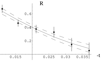
Figure 1: The best fit to the ratio of the measured analyzing power as given at the Spin 2000 conference to the pure CNI analyzing power. The 1 $\sigma$ confidence band is shown by dashed curves.

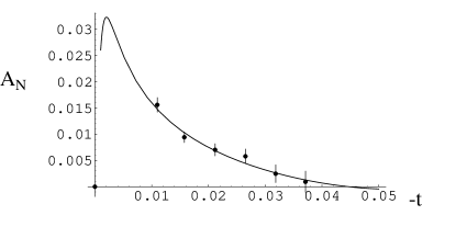
Figure 2: The best fit to the measured analyzing power as given at the Spin 2000 conference.

The best fit gives $Re[\,\tau(42)]=0.010$ and $Im[\,\tau(42)]=-0.038$; the errors on these two values are considerable and correlated, so we show the error ellipse in Fig. 3.

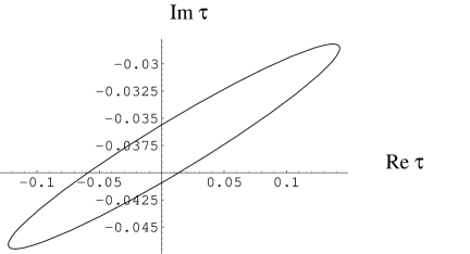
Figure 3: The 68.3% confidence level ellipse for the linear regression of the E950 data.

.

We see from this that $Re[\,\tau]$ is very uncertain; it is consistent with zero but could be bigger than 0.1 in magnitude with either sign. $Im[\,\tau]$ is much better determined, to within about 15% of its value; it is definitely not zero, and is negative. This better determination depends on the high sensitivity to $Im[\,\tau]$ of the prediction of the analyzing power at higher $|t|$. Now we use Eq.(10) and Eq.(11) to solve for $\tau_{P}$ and $\tau_{R}=\tau_{f}=\tau_{\omega}$, by our assumption. The results for the central values are $\tau_{P}=0.064$ and $\tau_{R}=-0.078$. The error ellipse is shown in Fig.4; the error on $\tau_{R}-\tau_{P}$ is relatively small because it is determined by $Im[\,\tau(42)]$. The error on $\tau_{P}$ itself is quite large; it is consistent with asymptotic spin dependence vanishing or being as large as 15%.

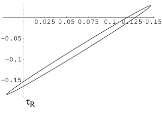
Figure 4: The 68.3% confidence level ellipse for the Regge spin-flip couplings $\tau_{P}$ and $\tau_{R}$ .

It is more interesting now to see the implication for the near term RHIC measurements with 100 GeV and 250 GeV proton beams on a fixed target. In this range both $Re[\,\tau(s)]$ and $Im[\,\tau(s)]$ vary, but not by enormous amounts. This is shown in Fig. 5.

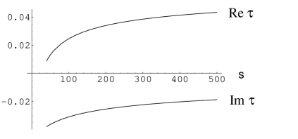
Figure 5: The energy dependence of the real and the imaginary parts of the pC spin-flip factor over the RHIC energy range.

The ratios to pure CNI, as in Fig. 1, are given in Fig. 6 and the corresponding plots of $A_{N}$ in Fig. 7.

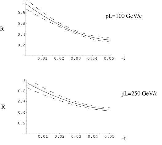
Figure 6: The ratio of the predicted analyzing power to pure CNI at $p_{L}=100\,GeV/c$ and $p_{L}=250\,GeV/c$ compared to the best fit curve at $p_{L}=21.7\,GeV/c$. The 1 $\sigma$ bands are also shown.

The asymptotic values will be eventually $Re[\,\tau(s)]=0.064$ while $Im[\,\tau(s)]$ will vanish; we see that we are a long way from that situation.

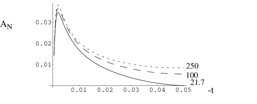
Figure 7: The predicted analyzing power at $p_{L}=100\,GeV/c$ and $p_{L}=250\,GeV/c$ compared to the best fit curve at $p_{L}=21.7\,GeV/c$.

3

Does this analysis teach us anything about the $pp$ analyzing power in the RHIC energy range? As pointed out at the beginning, the $I=1$ contribution is missing from $pC$ scattering; although it is known that, even as low as the E950 energy, the non-flip $I=1$ is small, the $I=1$ flip is very likely not to be small. It is well-known from Regge fits to $\pi p$ scattering that the $\rho$ spin-flip coupling is very large. Indeed, from the global fits done by Irving and Worden [6] the $I=1$ spin-flip Regge couplings are taken to be nearly an order of magnitude larger than the $I=1$ non-flip couplings. These are used in the analysis of Berger et al [5].

We can determine the error ellipse for the E704 data and compare it with the ellipse projected to $s=400$ for the $I=0$ piece from the $pC$ fits above. This is shown in Fig.8. Even though the E704 error ellipse is enormous, the central values, especially for $Im[\,\tau]$, are so different that there is no overlap of the two regions. The same remains true if we enlarge the ellipses to $90\%$ confidence level.

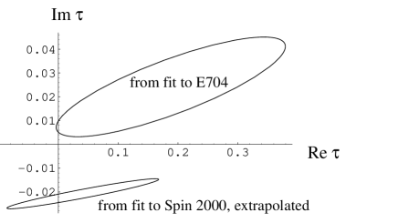
Figure 8: Ellipse from fitting E704 data compared to pC ellipse extrapolated to the same energy.

The data is too uncertain to try to do a serious fit to determine the $I=1$ piece from this difference. However, if one assumes that the Pomeron coupling is well determined from the $pC$ data because it is $I=0$, then we can try the same three Regge pole model and determine the size of the $C=+1$ and $C=-1$ Regge coupling (summing both iso-spins) and find that for $C=+1$, $\tau_{+}=0.53$ and for $C=-1$, $\tau_{-}=-1.03$. These are to be compared with the $I=0$ Regge coupling determined in Section 3: $\tau_{R}=-0.078$, evidently about an order of magnitude smaller, consistent with ancient expectations.

4

The results presented here must be considered to be preliminary. The numerical work has been checked by me several times, but not by anyone else. This all needs to be done more carefully when more data becomes available, which is expected to be soon. The parameters found are quite small but for larger $|t|$ for carbon (or any heavier nuclear target) the modification from pure CNI is large. Since the analysis here uses only the statistical errors, it seems likely that, in the small $t$-region, near the peak, the experimental uncertainty will be larger than the effects calculated here, which are less than $\approx 10\%$. Of course, this would be a useful result and is probably not very sensitive to the details of the model.

The Regge model used in the first section is fairly standard, but as with all Regge models, is pure phenomenology and the magnitude of the parameters are not calculable. As soon as data becomes available at a higher energy, the determinations described there can be carried through and, possibly, checked for use at higher energy. The model described in the second section is more speculative, requiring the assumption that $\tau_{f}=\tau_{\omega}$ ; this is unknown but is not unreasonable, and it allows us to make quantitative predictions for higher energy, just based on the E950 data. All of the quantitative results in Section 2 and Section 3 depend on it. We will soon know if it is wrong, but in the short term it may provide some guidance regarding reasonable expectations for energy dependence. The values of the spin-flip Regge couplings hold intrinsic interest for subsequent phenomenology and, possibly, for eventual understanding of the spin-dependence of Regge couplings.

I would like to thank Nigel Buttimore and Boris Kopeliovich for very helpful comments on this note.

References

- [1] J.R. Cudell et al, Phys.Rev.D61:034019 (2000), Erratum-ibid.D63:059901 (2001).
- [2] M.M. Block et al, hep-ph/9412306.
- [3] see, for example, pdg.lbl.gov.
- [4] B.Z. Kopeliovich and T.L. Trueman, Phys.Rev.D64:034004 (2001).
- [5] E.L. Berger, A.C. Irving, C. Sorenson, Phys.Rev.D17,2971 (1978).
- [6] A. Irving and R. Worden, Phys. Rep.34C, 117 (1977).
- [7] K. Kurita, private communication.
- [8] N.H. Buttimore et al, Phys.Rev.D59:114010 (1999).
- [9] B.Z. Kopeliovich and A.V. Tarasov, Phys.Lett.B497:44-48 (2001).