Verification of CPT–invariance of QED bound states for the production of muonium or antimuonium in scattering of electrons or positrons by nuclei

Abstract

A possibility of a verification of CPT–invariance of QED for bound states by example of muonium or antimuonium produced in reactions of scattering of electrons or positrons by nuclei is considered. The number of events of the muonium production is estimated for contemporary accelerators. The method of the detection of muonium by measuring of oscillations of the decay curve caused by the interference between the ground and excited state of muonium is suggested. The admixture of the excited muonium to the final state is calculated.

Department of Theoretical Physics, State Technical University of St. Petersburg,
195251 St. Petersburg, Russian Federation

1 Introduction

The verification of CPT–invariance of a quantum field theory (QFT) (in particular, Quantum Electrodynamics (QED)) is a meaningful problem of high energy physics, since the postulates of QFT are locality and relativistic invariance [1,2]. As has been shown in Ref.[3], this leads to invariance of the Lagrangian with respect to C–, P– and T–invariance. The simplest consequence CPT–invariance, the equality of masses of a particle and its antiparticle, is verified at present with a great accuracy. For example, for the masses of $\mu^{+}$ and $\mu^{-}$ one has $m_{\mu^{+}}/m_{\mu^{-}}=1.000024\pm 0.000078$ [4]. However, the problem of CPT–invariance of bound states is still much less clarified. For example, in Ref.[5] there has been suggested to treat the production of the antihydrogen for $\bar{p}Z$ collisions with a subsequent analysis of Lamb shifts $2S_{1/2}-2P_{1/2}$ of the transitions between hydrogen and antihydrogen. However, nowadays the available statistics of events is n ot enough to make a definite conclusion. It is smaller compared with the required by a factor 40.

2 Cross section for reactions (1)

In this paper we suggest to treat the production of a muonium $M^{0}$ or antimuonium $\bar{M}^{0}$ in reactions

$$e^{-}+Z\to Z+M^{0}+\mu^{-}\quad,\quad e^{+}+Z\to Z+\bar{M}^{0}+\mu^{+},$$ (2.1)

where $M^{0}(\bar{M}^{0})$ is a bound state of $\mu^{+}$, $e^{-}$ ($\mu^{-}$, $e^{+}$). The dominant contribution to the amplitude of reactions (2.1) comes from the diagrams depicted in Fig.1.

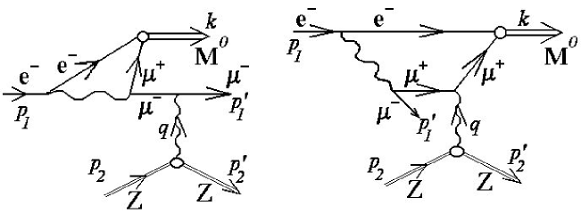
Figure 1: Feynman diagrams giving the dominant contribution to the amplitude of reactions (2.1)

Before we have written the amplitude of the reactions (2.1)(we would make everything by example of the reaction $e^{-}Z\to ZM^{0}\mu^{-}$) we suggest to discuss the vertex of recombination $e^{-}+\mu^{+}\to M^{0}$, $e^{+}+\mu^{-}\to\bar{M}^{0}$. This vertex has been derived in [6] within the Bethe–Salpeter equation with a kernel approximated by the one–photon exchange. The set diagrams depicting this kernel is given in Fig.2 .

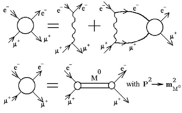
Figure 2: The Bethe–Salpeter equation in the diagrammatic form.

If for the diagrams in Fig.1 to denote the product of the Green function of electron $\hat{G}_{e^{-}}(p)=1/(\hat{p}-m_{e})$, the vertex of recombination $e^{-}+\mu^{+}\to M^{0}$, $\hat{\Gamma}_{0}$, and the Green function of the $\mu^{+}$–meson $\hat{G}_{\mu^{+}}(k-p)=1/(\hat{p}-\hat{k}-m_{\mu})$ as the quantity

$$\hat{X}(p,k-p)=\hat{G}_{\mu^{+}}(k-p)\,\hat{\Gamma}_{0}\,\hat{G}_{e^{-}}(p),$$ (2.2)

the solution of the Bethe–Salpeter equation for $\hat{X}(p,k-p)$ one can represent in the form [6]

$$\hat{X}(p,k-p)=(1-\gamma_{0})\gamma_{5}\frac{\sqrt{m_{\mu}}}{2\,i}\frac{\displaystyle\Big{(}\frac{\vec{p}^{\,2}}{2m_{e}}-E_{bound}\Big{)}\,\Phi(\vec{p}\,)}{\displaystyle\Big{(}p_{0}-m_{e}-\frac{\vec{p}^{\,2}}{2m_{e}}+i\,0\Big{)}\Big{(}p_{0}-k_{0}+m_{\mu}+\frac{\vec{p}^{\,2}}{2m_{\mu}}-i\,0\Big{)}},$$ (2.3)

such as the Fourier transform of the wave function of the electron in $M^{0}$ reads

$$\Phi(\vec{p}\,)=\frac{8\sqrt{\pi a^{3}_{0}}}{(1+p^{2}\,a^{2}_{0})^{2}},$$

where $a_{0}=1/m_{e}\alpha$ with $\alpha=e^{2}/4\pi$ is the fine structure constant defined in units $\hbar=c=1$.

Taking into account the diagrams in Fig.1 and using the vertex (2.3), we obtain the amplitude of the reaction (2.1) with $e^{-}$ in the following form

$$M=\frac{(4\pi\alpha)^{2}}{q^{2}}\,\Psi(0)\,{\ell}_{\nu}\,\frac{\sqrt{m_{\mu}}}{m_{e}\,(\omega^{2}-2q\cdot k)^{2}(q^{2}-2q\cdot k)}\,\bar{u}(p\,^{\prime}_{1})\,\gamma_{5}\,\Big{\{}2(2q\cdot k-\omega^{2})\,(q\cdot p\,^{\prime}_{1}\,\gamma_{\mu}$$

$$~{}~{}~{}-\hat{q}\,p\,^{\prime}_{1\mu})+m_{\mu}\,[(q^{2}-2q\cdot k)\,(2\,p\,^{\prime}_{1\mu}-\gamma_{\mu}\hat{q})-(\omega^{2}-2q\cdot k)\,(\hat{q}\,\gamma_{\mu}-2\,k_{\mu})]\Big{\}}\,u(p_{1}),$$ (2.4)

where $m_{e}$ and $m_{\mu}$ are masses of the electron and $\mu$–meson, respectively, $\omega^{2}=(p\,^{\prime}_{1}+k)^{2}$ is the squared invariant mass of $(M^{0},\mu^{-})$ system, ${\ell}_{\mu}$ is the electromagnetic current of the nucleus, and $\Psi(0)=1/\sqrt{\pi a^{3}_{0}}$.

The squared amplitude would involve the tensor $R_{\mu\nu}$ describing the lower block of the diagrams in Fig.1 containing the electromagnetic form factors of the nucleus $F_{1Z}$ and $F_{2Z}$:

$$R_{\mu\nu}=4\Big{\{}F^{2}_{1Z}(q^{2})\,\Big{[}2\,p_{2\mu}p_{2\nu}-(p_{2\mu}q_{\nu}+p_{2\nu}q_{\mu})+\frac{1}{2}\,q^{2}\,g_{\mu\nu}\Big{]}$$

$$+F^{2}_{2Z}(q^{2})\,\Big{[}2\,q^{2}\,m^{2}_{Z}\,g_{\mu\nu}+q^{2}\,(p_{2\mu}q_{\nu}+p_{2\nu}q_{\mu})-q_{\mu}q_{\nu}\,\Big{(}\frac{1}{2}\,q^{2}+2\,m^{2}_{Z}\Big{)}-2\,q^{2}\,p_{2\mu}p_{2\nu}\Big{]}\Big{\}}.$$ (2.5)

Let us introduce $x=\cos\theta$, where $\theta$ is a polar angle of the momentum of $M^{0}$ defined in the center of mass frame (CMF) of the system $(M^{0},\mu^{-})$ relative to the momentum of the electron in the CMF $(e^{-},Z)$. Using Eqs.(2) and (2) one can easily get the differential cross section with respect to $\omega^{2}$ and $x$ which reads

$$\frac{d^{2}\sigma}{d\omega^{2}dx} = 4\,F^{2}_{1Z}(0)\,|\Psi(0)|^{2}\pi\,\alpha^{4}\,\frac{m_{\mu}}{m^{2}_{e}}\,\sqrt{1-\frac{4m^{2}_{\mu}}{\omega^{2}}}\,{\ell n}\Big{(}\frac{s^{3}}{m^{2}_{Z}\omega^{4}}\Big{)}\,\frac{1}{\displaystyle 1+x\,\sqrt{1-\frac{4m^{2}_{\mu}}{\omega^{2}}}}$$ (2.6)

$$\times\,\frac{s-\omega^{2}}{s\,\omega^{6}}\left\{1+\frac{\displaystyle 8m^{2}_{\mu}\sqrt{1-\frac{4m^{2}_{\mu}}{\omega^{2}}}\Big{[}(1-x^{2})\sqrt{1-\frac{4m^{2}_{\mu}}{\omega^{2}}}+2\,x\Big{]}}{\displaystyle\omega^{2}\Big{[}1-x^{2}\Big{(}1-\frac{4m^{2}_{\mu}}{\omega^{2}}\Big{)}\Big{]}\,\Big{(}1-x\,\sqrt{1-\frac{4m^{2}_{\mu}}{\omega^{2}}}\Big{)}^{2}}\right\},$$

where $F_{1Z}(0)=Z$. The expression (2.6) is calculated within the Weizsäcker–Williams approach. One can see from Eq.(2.6) that in the CMF ($M^{0},\mu^{-}$) the muonium produces itself mainly backward. After the integration of (2.6) over $x$ one obtains the differential cross section with respect to $\omega^{2}$:

$$\frac{d\sigma}{d\omega^{2}}=2\,Z^{2}\,\alpha^{7}\,\Big{(}\frac{m_{e}}{m_{\mu}}\Big{)}\,\sqrt{1-\frac{4m^{2}_{\mu}}{\omega^{2}}}\,{\ell n}\Big{(}\frac{s^{3}}{m^{2}_{Z}\omega^{4}}\Big{)}\,\frac{s-\omega^{2}}{s\omega^{4}}\Bigg{\{}1-12\,\frac{m^{2}_{\mu}}{\omega^{2}}$$

$$+\left[4\,\left(\frac{m^{2}_{\mu}}{\omega^{2}}\right)^{2}\left(1-6\,\frac{m^{2}_{\mu}}{\omega^{2}}\right)+2\,\frac{m^{2}_{\mu}}{\omega^{2}}\right]\,\frac{1}{\displaystyle\sqrt{1-4m^{2}_{\mu}/\omega^{2}}}\,{\ell n}\frac{1+\sqrt{1-4m^{2}_{\mu}/\omega^{2}}}{1-\sqrt{1-4m^{2}_{\mu}/\omega^{2}}}\Bigg{\}}.$$ (2.7)

From Eq.(2) one gets that the maximum of the cross section is located in the vicinity of the threshold of the $(M^{0},\mu^{-})$–system production, $\omega^{2}\sim 4\,m^{2}_{\mu}$, and the quantity $d\sigma/d\omega^{2}$ falls substantially with $\omega^{2}$ and behaves like $d\sigma/d\omega^{2}\sim 1/\omega^{4}$.

Let us now obtain the total cross section of the reactions (2.1). For this aim we introduce a variable $\xi=4m^{2}_{\mu}/\omega^{2}$ and integrate (2) over $\xi$. This yields

$$\sigma=\Big{(}\frac{Z^{2}\alpha^{7}m_{e}}{16\,m^{3}_{\mu}}\Big{)}\int\limits^{1}_{0}f(\xi)\,d\xi,$$

$$f(\xi)={\ell n}\Bigg{(}\frac{s^{3}\xi^{2}}{16m^{2}_{Z}m^{4}_{\mu}}\Bigg{)}\,\left\{2\,(4-3\,\xi^{2})\sqrt{1-\xi}+\xi\,(4+2\,\xi-\xi^{2})\,{\ell n}\left(\frac{1+\sqrt{1-\xi}}{1-\sqrt{1-\xi}}\right)\right\}\!.$$ (2.8)

Let us estimate the values of the cross sections for the reactions (2.1) for Tevatron–DIS (FNAL) [8] and LHC [9] (we mean the beams of daughter leptons). The cross section is proportional to $Z^{2}$. Hence, it can be enhanced by using the target with a big $Z$ [5], for example, Radon ${{}^{220}}{\rm Rn}_{86}$ having a spin $1/2$. The values of the cross sections, different luminosities and an expected number of events for one year are adduced in Table.

Table. The data for the cross sections for the reactions (2.1) and the expected number of events for one year.

Accelerator	$\sqrt{s}$, GeV	$\sigma$, fb	L, ${\rm cm^{-2}\,s^{-1}}$	N
FNAL (Tevatron–DIS)	477	17	$2.1\times 10^{32}$	$1.1\times 10^{2}$
LHC	14000	28	$10^{33}-10^{34}$	$8.8\times 10^{2}-8.8\times 10^{3}$

3 Method of detection and estimate of admixture of excited states of muonium and antimuonim

Let us consider the method of the detection of the muonium $M^{0}$ and antimuonium $\bar{M}^{0}$. For the reactions (2.1) $M^{0}$ and $\bar{M}^{0}$ would be production both in the ground state and in the excited one as well

$$\Psi_{M^{0}}(0)=C_{1}\Psi_{1}(0)+C_{2}\Psi_{2}(0).$$ (3.1)

Emphasize that the solution of the Bethe–Salpeter equation (2.3) has been obtained for the production of the muonium in the ground state. The mechanisms of the production of an excited muonium, from which there follows that the coefficient $C_{2}$ contains an additional small parameter, would be discussed below. Taking into account the decay of muonium, the partial width of which we denote as $\Gamma_{M^{0}}$, one can represent the wave function of muonium in the form

$$\Psi_{M^{0}}(t)=\Big{(}C_{1}\Psi_{1}(t)+C_{2}\Psi_{2}(t)\Big{)}\,\exp\Big{(}-\frac{\Gamma_{M^{0}}t}{2\,\hbar}\Big{)}.$$ (3.2)

Here $\Psi_{1}(t)$ and $\Psi_{2}(t)$ are defined by

$$\Psi_{1}(t)=\Psi_{1}\,\exp\Big{(}-\frac{i}{\hbar}\,E_{1}t\Big{)}\quad,\quad\Psi_{2}(t)=\Psi_{2}\,\exp\Big{(}-\frac{i}{\hbar}\,E_{2}t\Big{)},$$ (3.3)

where $E_{1}$ and $E_{2}$ are the energies of muonium in the ground and excited states, then $\Gamma_{M^{0}}=\hbar/\tau_{M^{0}}$ with $\tau_{M^{0}}\sim 10^{6}\,sec$ is the mean life of muonium.

Taking into account that the wave function of muonium is normalized to the current density and introducing the power of the polarization $\varepsilon=|C_{2}|^{2}/|C_{1}+C_{2}|^{2}$, it is not difficult to calculate the current density of $M^{0}$ at an arbitrary time $t$ [7]:

$$I(t)=I_{0}\,\left\{1-2\,\sqrt{\varepsilon}\,(1-\sqrt{\varepsilon})\left[1-\cos\left(\frac{E_{2}-E_{1}}{\hbar}\,t\right)\right]\right\}\,\exp\left(-\frac{\Gamma_{M^{0}}t}{\hbar}\right).$$ (3.4)

It is seen that the decay curve $I(t)$ depicted in Fig.3 contains oscillations. Let us estimate the period of oscillations (the distance on which the curve in Fig.3 contains only one oscillation in time). Using (3.4), denoting $\omega=(E_{2}-E_{1})/\hbar=2\pi/T$ and accounting for that $E_{2}-E_{1}=10.1\,{\rm eV}$ one obtains $T\approx 4\times 10^{-16}\,$s. When matching $T$ with $\tau_{M^{0}}$ one can see that the period of oscillations in time is smaller compared with $\tau_{M^{0}}$ by ten orders of magnitude. The former means that in Fig.3 there should be a lot of oscillations for the mean life of $M^{0}$.

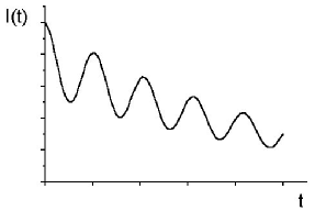
Figure 3: The decay curve of muonium with account for the excited state.

Since muonium produces in the reaction (2.1) with $E_{M^{0}}\gg m_{M^{0}}c^{2}$, for example, for Tevatron–DIS one gets $E_{M^{0}}\sim 225\,{\rm MeV}$, so $T_{\ell ab}=T(E_{M^{0}}/m_{M^{0}}c^{2})\approx 10^{-12}\,{\rm s}$. For this time muonium should be moved for the distance comeasurable with a space period of oscillations equal to approximately 300$\,mkm$. Effects on such distances are measurable.

Let us estimate the value of $\varepsilon$ defining the contribution of the wave function $\Psi_{2}$ to the formula (3.2) due to the production of muonium at the excited state $M^{0*}$. There are two mechanisms of the production of $M^{0*}$: (i) the production at the vertex of recombination $e^{-}+\mu^{+}\to M^{0*}$ in the diagrams in Fig.1 and (ii) interaction in the final state when $M^{0}$ rescatters inelastically by either $\mu^{-}$ or the nucleus. Consider the first mechanism. Let $M^{0}$ be produced at the $2\,{{}^{1}}{\rm S}_{0}$–state. In this case the equality (2.3) would contain $\Phi(\vec{p}\,)$ defined by

$$\Phi(\vec{p}\,)=-\frac{32\sqrt{2\pi a^{3}_{0}}\,(1-4\,\vec{p}^{\,2}\,a^{2}_{0})}{(1+4\,\vec{p}^{\,2}\,a^{2}_{0})^{3}},$$ (3.5)

where $a_{0}$ has been determined above and $\Psi(0)=1/\sqrt{8\pi a^{3}_{0}}$. This leads to the value $\varepsilon=1/256$ which means that the admixture of the excited state $\Psi_{2}$ in Eq.(3.2) is of order $10\,\%$. In the case of the $M^{0*}$ production at one of the $2P$–states the value of $\varepsilon$ turns out to be of the same order. The second mechanism gives a contribution substantially less.

Thus, a comparison of the decay curves of muonium and antimuonium for a few periods of oscillations should give a possibility to check whether there exists CPT–invariance for bound states in QED.

References

- [1] A. I. Achiezer and V. B. Berestetskii, in QUANTUM ELECTRODYNAMICS, Nauka, 1969.
- [2] N. N. Bogoliubov and D. V. Shirkov, in INTRODUCTION TO THEORY OF QUANTUM FIELDS, Nauka, 1976.
- [3] R. Jost, in GENERAL THEORY OF QUANTUM FIELDS, 1967.
- [4] D. E. Groom et al., Eur. Phys. J. C15, 1 (2000).
- [5] C. T. Munger, S. J. Brodsky, and I. Schmidt, Phys. Rev. D49, 3228 (1994).
- [6] E. A. Choban, Proceedings of SPIE, 3345, 162 (1997)
- [7] E. A. Choban, Proceedings of XXXIV Winter School of Petersburg Nuclear Physics Institute (Physics of Atomic Nucleus and Elementary Particles), pp. 498–510, 2000.
- [8] CERN Yellow Report, 4, 25 (2000).
- [9] P. Chiapetta et al., Phys. Rev. D59, 014016 (1999).