SACLAY-T02/024

THE COLOUR GLASS CONDENSATE:
AN INTRODUCTION

Edmond Iancu
Service de Physique Théorique
CE Saclay, F-91191 Gif-sur-Yvette, France

Andrei Leonidov
P. N. Lebedev Physical Institute, Moscow, Russia

Larry McLerran
Nuclear Theory Group, Brookhaven National Laboratory
Upton, NY 11793, USA

Abstract: In these lectures, we develop the theory of the Colour Glass Condensate. This is the matter made of gluons in the high density environment characteristic of deep inelastic scattering or hadron-hadron collisions at very high energy. The lectures are self contained and comprehensive. They start with a phenomenological introduction, develop the theory of classical gluon fields appropriate for the Colour Glass, and end with a derivation and discussion of the renormalization group equations which determine this effective theory.

1 General Considerations

1.1 Introduction

The goal of these lectures is to convince you that the average properties of hadronic interactions at very high energies are controlled by a new form of matter, a dense condensate of gluons. This is called the Colour Glass Condensate since

• Colour: The gluons are coloured.

• Glass: The associated fields evolve very slowly relative to natural time scales, and are disordered. This is like a glass which is disordered and is a liquid on long time scales but seems to be a solid on short time scales.

• Condensate: There is a very high density of massless gluons. These gluons can be packed until their phase space density is so high that interactions prevent more gluon occupation. With increasing energy, this forces the gluons to occupy higher momenta, so that the coupling becomes weak. The gluon density saturates at a value of order $1/\alpha_{s}\gg 1$, corresponding to a multiparticle state which is a Bose condensate.

In these lectures, we will try to explain why the above is very plausible.

Before doing this, however, it is useful to review some of the typical features of hadronic interactions, and some unanswered theoretical questions which are associate with these phenomena. This will motivate much of the later discussion.

1.2 Total Cross Sections at Asymptotic Energy

Computing total cross sections as $E\rightarrow\infty$ is one of the great unsolved problems of QCD. Unlike for processes which are computed in perturbation theory, it is not required that any energy transfer become large as the total collision energy $E\rightarrow\infty$. Computing a total cross section for hadronic scattering therefore appears to be intrinsically non-perturbative. In the 60’s and early 70’s, Regge theory was extensively developed in an attempt to understand the total cross section. The results of this analysis were to our mind inconclusive, and certainly can not be claimed to be a first principles understanding from QCD.

Figure 1: The cross sections for $pp$ and $p\overline{p}$ scattering.

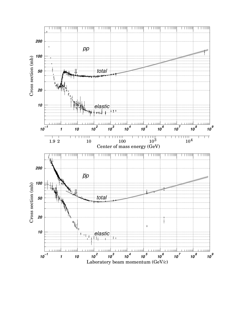
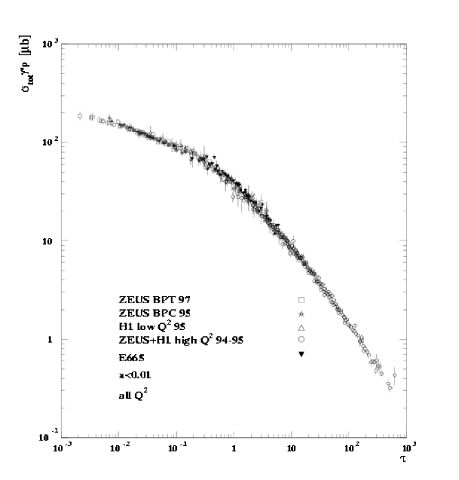
The total cross section for $pp$ and $\overline{p}p$ collisions is shown in Fig. 1. Typically, it is assumed that the total cross section grows as $\ln^{2}E$ as $E\rightarrow\infty$. This is the so called Froissart bound, which corresponds to the maximal growth allowed by the unitarity of the scattering matrix. Is this correct? Is the coefficient of $\ln^{2}E$ universal for all hadronic precesses? Why is the unitarity limit saturated? Can we understand the total cross section from first principles in QCD? Is it understandable in weakly coupled QCD, or is it an intrinsically non-perturbative phenomenon?

1.3 Particle Production in High Energy Collisions

In order to discuss particle production, it is useful to introduce some kinematical variables adapted for high energy collisions: the light cone coordinates. Let $z$ be the longitudinal axis of the collision. For an arbitrary 4-vector $v^{\mu}=(v^{0},v^{1},v^{2},v^{3})$ ($v^{3}=v_{z}$, etc.), we define its light-cone (LC) coordinates as

$$v^{+}\equiv{1\over\sqrt{2}}(v^{0}+v^{3}),\qquad v^{-}\equiv{1\over\sqrt{2}}(v^{0}-v^{3}),\qquad v_{\perp}\equiv(v^{1},v^{2}).$$ (1.1)

In particular, we shall refer to $x^{+}=(t+z)/\sqrt{2}$ as the LC “time”, and to $x^{-}=(t-z)/\sqrt{2}$ as the LC “longitudinal coordinate”. The invariant dot product reads:

$$p\cdot x\,=\,p^{-}x^{+}+p^{+}x^{-}-p_{\perp}\cdot x_{\perp},$$ (1.2)

which suggests that $p^{-}$ — the momentum variable conjugate to the “time” $x^{+}$ — should be interpreted as the LC energy, and $p^{+}$ as the (LC) longitudinal momentum. In particular, for particles on the mass-shell: $p^{\pm}=(E\pm p_{z})/\sqrt{2}$, with $E=(m^{2}+{\bf p}^{2})^{1/2}$, and therefore:

$$p^{+}p^{-}\,=\,{1\over 2}(E^{2}-p_{z}^{2})={1\over 2}(p_{\perp}^{2}+m^{2})\,=\,{1\over 2}\,m_{\perp}^{2}\,.$$ (1.3)

This equation defines the transverse mass $m_{\perp}$. We shall also need the rapidity :

$${\rm y}\,\equiv\,{1\over 2}\ln\frac{p^{+}}{p^{-}}={1\over 2}\ln{2p^{+2}\over m_{\perp}^{2}}.$$ (1.4)

These definitions are useful, among other reasons, because of their simple properties under longitudinal Lorentz boosts: $p^{+}\rightarrow\kappa p^{+}$, $p^{-}\rightarrow(1/\kappa)p^{-}$, where $\kappa$ is a constant. Under boosts, the rapidity is just shifted by a constant: ${\rm y}\rightarrow{\rm y}+\kappa$.

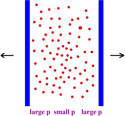
Consider now the collision of two identical hadrons in the center of mass frame, as shown in Fig. 2. In this figure, we have assumed that the colliding hadrons have a transverse extent which is large compared to the size of the produced particles. This is true for nuclei, or if the typical transverse momenta of the produced particles is large compared to $\Lambda_{QCD}$, since the corresponding size will be much smaller than a Fermi. We have also assumed that the colliding particles have an energy which is large enough so that they pass through one another and produce mesons in their wake. This is known to happen experimentally: the particles which carry the quantum numbers of the colliding particles typically lose only some finite fraction of their momenta in the collision. Because of their large energy, the incoming hadrons propagate nearly at the speed of light, and therefore are Lorentz contracted in the longitudinal direction, as suggested by the figure.

Figure 2: A hadron-hadron collision. The produced particles are shown as circles.

In LC coordinates, the right moving particle (“the projectile”) has a 4-momentum $p_{1}^{\mu}=(p_{1}^{+},p_{1}^{-},0_{\perp})$ with $p^{+}_{1}\simeq\sqrt{2}p_{z}$ and $p_{1}^{-}=M^{2}/2p^{+}_{1}$ (since $p_{z}\gg M$, with $M=$ the projectile mass). Similarly, for the left moving hadron (“the target”), we have $p^{+}_{2}=p^{-}_{1}$ and $p^{-}_{2}=p^{+}_{1}$. The invariant energy squared is $s=(p_{1}+p_{2})^{2}=2p_{1}\cdot p_{2}\simeq 2p^{+}_{1}p^{-}_{2}\simeq 4p_{z}^{2}$, and coincides, at it should, with the total energy squared $(E_{1}+E_{2})^{2}$ in the center of mass frame.

We define the longitudinal momentum fraction, or Feynman’s ${\rm x}$, of a produced pion as

$${\rm x}\,\equiv\,\frac{p^{+}_{\pi}}{p_{1}^{+}}$$ (1.5)

(with $0<{\rm x}\leq 1$). The rapidity of the pion is then

$${\rm y}\,=\,{1\over 2}\ln{p^{+}_{\pi}\over p^{-}_{\pi}}={1\over 2}\ln{2p^{+2}_{\pi}\over m_{\perp}^{2}}\,=\,{\rm y}_{proj}-\ln{1\over{\rm x}}+\ln{M\over m_{\perp}},$$ (1.6)

where ${\rm y}_{proj}=\ln(\sqrt{2}{p^{+}_{1}/M})=\ln(\sqrt{s}/M)$. The pion rapidity is in the range $-{\rm y}_{proj}\mathrel{\hbox to0.0pt{\raise 2.20013pt\hbox{$<$}\hss}{\lower 2.20013pt\hbox{$\sim$}}}{\rm y}\mathrel{\hbox to0.0pt{\raise 2.20013pt\hbox{$<$}\hss}{\lower 2.20013pt\hbox{$\sim$}}}{\rm y}_{proj}$ (up to an overall shift by $\Delta y=\ln(M/m_{\perp})$).

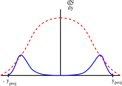
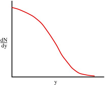
A typical distribution of produced particles (say, pions) in a hadronic collision is shown in Fig. 3. We denote by $dN/d{\rm y}$ the number of produced particles per unit rapidity. The leading particles are shown by the solid line and are clustered around the projectile and target rapidities. For example, in a heavy ion collision, this is where the nucleons would be. The dashed line is the distribution of produced mesons.

Figure 3: The rapidity distribution of particles produced in a hadronic collision.

Several theoretical issues arise in multiparticle production:

Can we compute $dN/d{\rm y}$ ? Or even $dN/d{\rm y}$ at ${\rm y}=0$ (“central rapidity”) ? How does the average transverse momentum of produced particles $\langle p_{\perp}\rangle$ behave with energy? What is the ratio of produced strange/nonstrange mesons, and corresponding ratios of charm, top, bottom etc at ${\rm y}=0$ as the center of mass energy approaches infinity? Does multiparticle production as $s\rightarrow\infty$ at ${\rm y}=0$ become simple, understandable and computable?

Note that ${\rm y}=0$ corresponds to particles with $p_{z}=0$ or $p^{+}=m_{\perp}/\sqrt{2}$, for which ${\rm x}=m_{\perp}/(\sqrt{2}p^{+}_{1})=m_{\perp}/\sqrt{s}$ is small, ${\rm x}\ll 1$, in the high-energy limit of interest. Thus, presumably, the multiparticle production at central rapidity reflects properties of the small-x degrees of freedom in the colliding hadron wavefunctions.

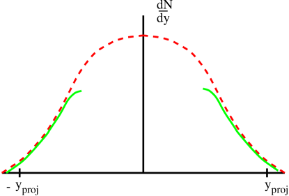
There is a remarkable feature of rapidity distributions of produced hadrons, which we shall refer to as Feynman scaling. If we plot rapidity distributions of produced hadrons at different energies, then as function of ${\rm y}-{\rm y}_{proj}$, the rapidity distributions are to a good approximation independent of energy. This is illustrated in Fig. 4, where the rapidity distribution measured at one energy is shown with a solid line and the rapidity distribution at a different, higher, energy is shown with a dotted line. (In this plot, the rapidity distribution at the lower energy has been shifted by an amount so that particles of positive rapidity begin their distribution at the same ${\rm y}_{proj}$ as the high energy particles, and correspondingly for the negative rapidity particles. This of course leads to a gap in the center for the low energy particles due to this mapping.)

This means that as we go to higher and higher energies, the new physics is associated with the additional degrees of freedom at small rapidities in the center of mass frame (small-x degrees of freedom). The large x degrees of freedom do not change much. This suggests that there may be some sort of renormalization group description in rapidity where the degrees of freedom at larger x are held fixed as we go to smaller values of x. We shall see that in fact these large x degrees of freedom act as sources for the small x degrees of freedom, and the renormalization group is generated by integrating out degrees of freedom at relatively large x to generate these sources.

Figure 4: Feynman scaling of rapidity distributions. The two different lines correspond to rapidity distributions at different energies.

1.4 Deep Inelastic Scattering

In Fig. 5, deep inelastic scattering is shown.

Figure 5: Deep inelastic scattering of an electron on a hadron.

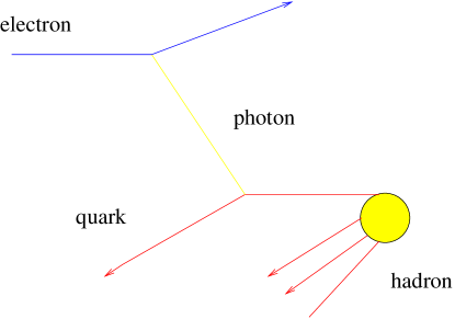
Here an electron emits a virtual photon which scatters from a quark in a hadron. The momentum and energy transfer of the electron is measured, but the results of the hadron break up are not. In these lectures, we do not have sufficient time to develop the theory of deep inelastic scattering (see, e.g., [1] for more details). For the present purposes, it is enough to say that, at large momentum transfer $Q^{2}\gg\Lambda_{QCD}^{2}$, this experiment can be used to measure the distributions of quarks in the hadron.

To describe the quark distributions, it is convenient to work in a reference frame where the hadron has a large light-cone longitudinal momentum $P^{+}\gg M$ (“infinite momentum frame”). In this frame, one can describe the hadron as a collection of constituents (“partons”), which are nearly on-shell excitations carrying some fraction x of the total longitudinal momentum $P^{+}$. Thus, the longitudinal momentum of a parton is $p^{+}={\rm x}P^{+}$, with $\,0\leq{\rm x}<1$.

For the struck quark in Fig. 5, this x variable (“Feynman’s x”) is equal to the Bjorken variable ${\rm x}_{Bj}$, which is defined in a frame independent way as ${\rm x}_{Bj}=Q^{2}/2P\cdot q$, and is directly measured in the experiment. In this definition, $Q^{2}=-q^{\mu}q_{\mu}$, with $q^{\mu}$ the (space-like) 4-momentum of the exchanged photon. The condition that ${\rm x}={\rm x}_{Bj}$ is what maximizes the spatial overlap between the struck quark and the virtual photon, thus making the interaction favourable.

The Bjorken variable scales like ${\rm x}_{Bj}\sim Q^{2}/s$, with $s=$ the invariant energy squared. Thus, in deep inelastic scattering at high energy (large $s$ at fixed $Q^{2}$) one measures quark distributions $dN_{quark}/d{\rm x}$ at small x (${\rm x}\ll 1$).

It is useful to think about these distributions as a function of rapidity. We define the rapidity in deep inelastic scattering as

$${\rm y}={\rm y}_{hadron}-\ln(1/{\rm x}),$$ (1.7)

and the invariant rapidity distribution as

$${dN\over d{\rm y}}\,={\,{\rm x}{dN\over d{\rm x}}}\,.$$ (1.8)

In Fig. 6, a typical $dN/d{\rm y}$ distribution for constituent gluons of a hadron is shown. This plot is similar to the rapidity distribution of produced particles in hadron-hadron collisions (see Fig. 3). The main difference is that, now, we have only half of the plot, corresponding to the right moving hadron in a collision in the center of mass frame.

Figure 6: The rapidity distribution of gluons inside of a hadron.

One may in fact argue that there is indeed a relationship between the structure functions as measured in deep inelastic scattering and the rapidity distributions for particle production. We expect, for instance, the gluon distribution function to be proportional to the pion rapidity distribution. This is what comes out in many models of particle production. It is further plausible, since the degrees of freedom of the gluons should not be lost, but rather converted into the degrees of freedom of the produced hadrons.

The small x problem is that in experiments at HERA, the rapidity distributions for quarks and gluons grow rapidly as the rapidity difference

$$\tau\,\equiv\,\ln(1/{\rm x})\,=\,{\rm y}_{hadron}-{\rm y}$$ (1.9)

between the quark and the hadron increases [2]. This growth appears to be more rapid than $\tau$ or $\tau^{2}$, and various theoretical models based on the original considerations by Lipatov and colleagues [3] suggest it may grow as an exponential in $\tau$ [3, 4]. The more established DGLAP evolution equation [5] predicts a less rapide growth, like an exponential in $\sqrt{\tau}$, but this is still exceeding the Froissart unitarity bound, which requires rapidity distributions to grow at most as $\tau^{2}$ (since $\tau\sim\ln s$).

Figure 7: The Zeus data for the gluon structure functions.

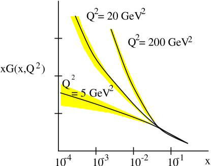
In Fig. 7, the ZEUS data for the gluon distribution are plotted for $Q^{2}=5~{}{\rm GeV}^{2}$, $20~{}{\rm GeV}^{2}$ and $200~{}{\rm GeV}^{2}$ [2]. The gluon distribution is the number of gluons per unit rapidity in the hadron wavefunction, ${\rm x}G({\rm x},Q^{2})=dN_{gluons}/d{\rm y}\;$. Experimentally, it is extracted from the data for the quark structure functions, by exploiting the dependence of the latter upon the resolution of the probe, that is, upon the transferred momentum $Q^{2}$. Note the rise of ${\rm x}G({\rm x},Q^{2})$ at small x: this is the small x problem. If one had plotted the total multiplicity of produced particles in $pp$ and $\overline{p}p$ collisions on the same plot, one would have found rough agreement in the shape of the curves.

Figure 8: Saturation of gluons in a hadron. A view of a hadron head on as x decreases.

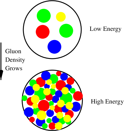
Why is the small x rise in the gluon distribution a problem? Consider Fig. 8, where we view the hadron head on. The constituents are the valence quarks, gluons and sea quarks shown as coloured circles. As we add more and more constituents, the hadron becomes more and more crowded. If we were to try to measure these constituents with say an elementary photon probe, as we do in deep inelastic scattering, we might expect that the hadron would become so crowded that we could not ignore the shadowing effects of constituents as we make the measurement. (Shadowing means that some of the partons are obscured by virtue of having another parton in front of them. This would result in a decrease of the scattering cross section relative to what is expected from incoherent independent scattering.)

We shall later argue that the distribution functions at fixed $Q^{2}$ saturate, which means that they cease growing so rapidly at high energy [6, 7, 8, 9, 10]. (See also Refs. [11, 12, 13, 14] for recent reviews and more references.) This saturation will be seen to occur at transverse momenta below some intrinsic scale, the “saturation scale”, which is estimated as:

$$Q_{s}^{2}\,=\,\alpha_{s}N_{c}\,{1\over{\pi R^{2}}}{{dN}\over{d{\rm y}}}\,,$$ (1.10)

where $dN/d{\rm y}$ is the gluon distribution. Only gluons matter since, at small x, the gluon density grows faster then the quark density, and is the driving force towards saturation. This is why in the forthcoming considerations we shall ignore the (sea) quarks, but focus on the gluons alone. Furthermore, $\pi R^{2}$ — with $R$ the hadron radius — is the area of the hadron in the transverse plane. (This is well defined as long as the wavelengths of the external probes are small compared to $R$.) Finally, $\alpha_{s}N_{c}$ is the colour charge squared of a single gluon. Thus, the “saturation scale” (1.10) has the meaning of the average colour charge squared of the gluons in the hadron wavefunction per unit transverse area.

Since the gluon distribution increases rapidly with the energy, as shown by the HERA data, so does the saturation scale. We shall use the rapidity difference $\tau=\ln(1/{\rm x})\sim\ln s$, eq. (1.9), to characterize this increase, and write $Q_{s}^{2}\equiv Q_{s}^{2}(\tau)$. For sufficiently large $\tau$ (i.e., high enough energy, or small enough x),

$$Q_{s}^{2}(\tau)\gg\Lambda^{2}_{QCD},$$ (1.11)

and $\alpha_{s}(Q_{s}^{2})\ll 1$. Then we are dealing with weakly coupled QCD, so we should be able to perform a first principle calculation of, e.g.,

• the gluon distribution function;

• the quark and heavy quark distribution functions;

• the intrinsic $p_{\perp}$ distributions of quarks and gluons.

But weak coupling does not necessarily mean that the physics is perturbative. There are many examples of nonperturbative phenomena at weak coupling. An example is instantons in electroweak theory, which lead to the violation of baryon number. Another example is the atomic physics of highly charged nuclei, where the electron propagates in the background of a strong nuclear Coulomb field. Also, at very high temperature, QCD becomes a weakly coupled quark-gluon plasma, but it exhibits nonperturbative phenomena on large distances $r\gg 1/T$ (with $T$ the temperature), due to the collective behaviour of many quanta [15].

Returning to our small-x gluons, we notice that, at low transverse momenta $Q^{2}\leq Q_{s}^{2}(\tau)$, they make a high density system, in which the interaction probability

$$\frac{\alpha_{s}(Q^{2})}{Q^{2}}\,{1\over{\pi R^{2}}}\,{{dN}\over{d{\rm y}}}\,\,\sim\,\,1\quad{\rm when}\quad Q^{2}\sim Q^{2}_{s}(\tau)$$ (1.12)

is of order one [6, 7, 16]. That is, although the coupling is small, $\alpha_{s}(Q^{2})\ll 1$, the effects of the interactions are amplified by the large gluon density (we shall see that $dN/d{\rm y}\sim 1/\alpha_{s}$ at saturation), and ordinary perturbation theory breaks down.

To cope with this, a resummation of the high density effects is necessary. Our strategy to do so — to be described at length in these lectures — will be to construct an effective theory in which the small-x gluons are described as the classical colour fields radiated by “colour sources” at higher rapidity. Physically, these sources are the “fast” partons, i.e., the hadron constituents with larger longitudinal momenta $p^{+}\gg{\rm x}P^{+}$. The properties of the colour sources will be obtained via a renormalization group analysis, in which the “fast” partons are integrated out in steps of rapidity and in the background of the classical field generated at the previous steps.

The advantage of this strategy is that the non-linear effects are dealt with in a classical context, which makes exact calculations possible. Specifically, (a) the classical field problem will be solved exactly, and (b) at each step in the renormalization group analysis, the non-linear effects associated with the classical fields will be treated exactly. On the other hand, the mutual interactions of the fast partons will be treated in perturbation theory, in a “leading-logarithmic” approximation which resums the most important quantum corrections at high energy (namely, those which are enhanced by the large logarithm $\ln(1/{\rm x})$).

As we shall see, the resulting effective theory describes the saturated gluons as a Colour Glass Condensate. The classical field approximation is appropriate for these saturated gluons, because of the large occupation number $N_{k}\sim 1/\alpha_{s}\gg 1$ of their true quantum state. In this limit, the Heisenberg commutators between particle creation and annihilation operators become negligible:

$$[a_{k},\,a^{\dagger}_{k}]\,=\,1\,\ll\,a^{\dagger}_{k}a_{k}=N_{k}\,,$$ (1.13)

which corresponds indeed to a classical regime. The classical field language is also well adapted to describe the coherence of these small-x gluons, which overlap with each other because of their large longitudinal wavelengths.

The phenomenon of saturation provides also a natural solution to the unitarity problem alluded to before. We shall see that, with increasing energy, the new partons are produced preponderently at momenta $p_{\perp}\mathrel{\hbox to0.0pt{\raise 2.20013pt\hbox{$>$}\hss}{\lower 2.20013pt\hbox{$\sim$}}}Q_{s}$. Thus, these new partons have a typical transverse size $\sim 1/p_{\perp}\mathrel{\hbox to0.0pt{\raise 2.20013pt\hbox{$<$}\hss}{\lower 2.20013pt\hbox{$\sim$}}}1/Q_{s}$. Smaller is x (i.e., larger is $\tau$), larger is $Q_{s}(\tau)$, and therefore smaller are the newly produced partons. An external probe of transverse resolution $\Delta x_{\perp}\sim 1/Q$ will not see partons smaller than this resolution size. For $\tau$ large enough, $Q^{2}<Q_{s}^{2}(\tau)$, so that the partons produced when further increasing the energy will not contribute to the cross section at fixed $Q^{2}$. Thus, although the gluon distribution keeps increasing with $\tau$, there is nevertheless no contradiction with unitarity.

1.5 Geometrical Scaling

Another striking feature of the experimental data at HERA is geometrical scaling at Bjorken ${\rm x}<0.01$ [17]. In general, one expects the structure functions extracted from deep inelastic scattering to depend upon two dimensionless kinematical variables, x and $Q^{2}/\Lambda^{2}$, where $\Lambda^{2}$ is some arbitrary momentum scale of reference, which is fixed. The striking feature alluded to before is the observation that the x dependence measured at HERA at ${\rm x}<0.01$ and for a broad region of $Q^{2}$ (between $0.045$ and $450\,{\rm Gev}^{2}$) can be entirely accounted for by a corresponding dependence of the reference scale $\Lambda^{2}\rightarrow 1/R^{2}({\rm x})$ alone. That is, rather than being functions of two independent variables x and $Q^{2}/\Lambda^{2}$, the measured structure functions at ${\rm x}<0.01$ depend effectively only upon the scaling variable

$${\cal T}\,\equiv\,Q^{2}R^{2}({\rm x})$$ (1.14)

where $R^{2}({\rm x})\sim{\rm x}^{\lambda}$ and $\lambda\sim 0.3-0.4$ in order to fit the data. This is illustrated in Fig. 9 [17].

Figure 9: Experimental data on the cross section for virtual photon-proton deep inelastic scattering from the region ${\rm x}<0.01$ plotted verses the scaling variable ${\cal T}=Q^{2}R^{2}({\rm x})$ [17].

Such a scaling behaviour is consistent with the saturation scenario [18, 10, 19], as we shall discuss towards the end of these lectures. Note however that the experimentally observed scaling extends to relatively large values of x and $Q^{2}$, above all the estimates for the saturation scale. Thus, this feature seems to be more general than the phenomenon of saturation.

1.6 Universality

There are two separate formulations of universality which are important in understanding small x physics.

a) The first is a weak universality [8, 10]. This is the statement that at sufficiently high energy, physics should depend upon the specific properties of the hadron at hand (like its size or atomic number $A$) only via the saturation scale $Q_{s}(\tau,A)$. Thus, at high energy, there should be some equivalence between nuclei and protons: When their $Q_{s}^{2}$ values are the same, their properties must be the same. An empirical parameterization of the gluon structure function in eq. (1.10) is

$${1\over{\pi R^{2}}}{{dN}\over{d{\rm y}}}\sim{{A^{1/3}}\over x^{\delta}}$$ (1.15)

where $\delta\sim 0.2-0.3$ [2]. This suggests the following correspondences:

• RHIC with nuclei $\sim$ HERA with protons;

• LHC with nuclei $\sim$ HERA with nuclei.

Estimates of the saturation scale for nuclei at RHIC energies give $\sim 1-2~{}{\rm Gev}$, and at LHC $Q_{s}\sim 2-3~{}{\rm Gev}$.

b) The second is a strong universality which is meant in a statistical mechanical sense. This is the statement that the effective action which describes small x distribution function is critical and at a fixed point of some renormalization group. This means that the behavior of correlation functions is given by universal critical exponents, which depend only on general properties of the theory such as its symmetries and dimensionality.

1.7 Some applications

We conclude these introductory considerations with a (non-exhaustive) enumeration of recent applications of the concept of saturation and the Colour Glass Condensate (CGC) to phenomenology.

Consider deep inelastic scattering first. It has been shown in Refs. [18] that the HERA data for (both inclusive and diffractive) structure functions can be well accounted for by a phenomenological model which incorporates saturation. The same model has motivated the search for geometrical scaling in the data, as explained in Sect. 1.5.

Coming to ultrarelativistic heavy ion collisions, as experimentally realized at RHIC and, in perspective, at LHC, we note that the CGC should be the appropriate description of the initial conditions. Indeed, most of the multiparticle production at central rapidities is from the small-x (${\rm x}\leq 10^{-3}$) partons in the nuclear wavefunctions, which are in a high-density, semi-classical, regime. The early stages of a nuclear collision, up to times $\sim 1/Q_{s}$, can thus be described as the melting of the Colour Glass Condensates in the two nuclei. In Refs. [20], this melting has been systematically studied, and the multiparticle production computed, via numerical simulations of the classical effective theory [8, 21]. After they form, the particles scatter with each other, and their subsequent evolution can be described by transport theory [22].

The first experimental data at RHIC [23] have been analyzed from the perspective of the CGC in Refs. [24, 25, 26]. Specifically, the multiparticle production has been studied with respect to its dependence upon centrality (“number of participants”) [24], rapidity [25] and transverse momentum distribution [26].

The charm production from the CGC in peripheral heavy-ion collisions has been investigated in [27].

Electron-nucleus ($eA$) deeply inelastic scattering has been recently summarized in [28]. Some implications of the Colour Glass Condensate for the central region of $p+A$ collisions have been explored in Refs. [29, 30].

Instantons in the saturation environment have been considered in Ref. [31].

2 The classical effective theory

With this section, we start the study of an effective theory for the small x component of the hadron wavefunction [8, 10, 32, 33, 34, 35, 36, 37] (see also the previous review papers [12, 38]). Motivated by the physical arguments exposed before, in particular, by the separation of scales between fast partons and soft (i.e., small-x) gluons, in the infinite momentum frame, this effective theory admits a rigourous derivation from QCD, to be described in Sect. 3. Here, we shall rather rely on simple kinematical considerations to motivate its general structure.

2.1 A stochastic Yang-Mills theory

In brief, the effective theory is a classical Yang-Mills theory with a random colour source which has only a “plus” component :

$$(D_{\nu}F^{\nu\mu})_{a}(x)\,=\,\delta^{\mu+}\rho_{a}(x)\,.$$ (2.1)

The classical gauge fields $A^{\mu}_{a}$ represent the soft gluons in the hadron wavefunction, i.e., the gluons with small longitudinal momenta ($k^{+}={\rm x}P^{+}$ with ${\rm x}\ll 1$). For these gluons, the classical approximation should be appropriate since they are in a multiparticle state with large occupation numbers.

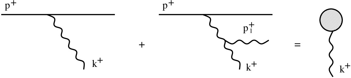
The fast partons, with momenta $p^{+}\gg k^{+}$, are not dynamical fields anylonger, but they have been rather replaced by the colour current $J^{\mu}_{a}=\delta^{\mu+}\!\rho_{a}$ which acts as a source for the soft gluon fields. This is quite intuitive: the soft gluons in the hadron wavefunction are radiated by typically fast partons, via the parton cascades shown in Fig. 10. It is in fact well known that, for the tree-level radiative process shown in Fig. 10.a, classical and quantum calculations give identical results in the limit where the emitted gluon is soft [1]. What is less obvious, but will be demonstrated by the analysis in Sect. 3, is that quantum corrections like those displayed in Fig. 10.b do not invalidate this classical description, but simply renormalize the properties of the classical source, in particular, its correlations.

Figure 10: a) Soft gluon emission by a fast parton; b) a gluon cascade.

The gross properties of this source follow from kinematics. The fast partons move along the $z$ axis at nearly the speed of light. They can emit, or absorb, soft gluons, but in a first approximation they preserve straightline trajectories along the light-cone ($z=t$). In terms of LC coordinates, they propagate in the positive $x^{+}$ direction, while sitting at $x^{-}=0$. Their colour current is proportional to their velocity, which implies $J_{a}^{\mu}=\delta^{\mu+}\!\rho_{a}$, with a charge density $\rho_{a}(x)$ which is localized near $x^{-}=0$. More precisely, as quantum fields, the fast partons are truly delocalized over a longitudinal distance $\Delta x^{-}\sim 1/p^{+}$, as required by the uncertainty principle. But since $1/p^{+}\ll 1/k^{+}$, they still look as sharply localized when “seen” by the soft gluons, which have long wavelengths and therefore a poor longitudinal resolution.

The separation of scales in longitudinal momenta implies a corresponding separation in time: Softer partons have larger energies, and therefore shorter lifetimes. Consider indeed the radiative process in Fig. 10.a, where $k^{+}\ll p^{+}$. This is a virtual excitation whose lifetime (in units of LC time $x^{+}$) can be estimated from the uncertainty principle as

$$\Delta x^{+}\,=\,\frac{1}{\varepsilon_{p-k}+\varepsilon_{k}-\varepsilon_{p}}\,\simeq\,\frac{1}{\varepsilon_{k}}\,\ll\,\frac{1}{\varepsilon_{p}}\,.$$ (2.2)

This is small as compared to the typical time scale $1/\varepsilon_{p}$ for the dynamics of the fast partons. [In eq. (2.2), $\varepsilon_{p}\equiv p_{\perp}^{2}/2p^{+}$ is the LC energy of the on-shell gluon with momentum ${\vec{p}}=(p^{+},{\bf p}_{\perp})$, and we have used the fact that, for $k^{+}\ll p^{+}$ and comparable transverse momenta $k_{\perp}$ and $p_{\perp}$, $\varepsilon_{k}\gg\varepsilon_{p},\varepsilon_{p-k}$.] Thus, the “fast” degrees of freedom are effectively frozen over the short lifetime of the soft gluon, and can be described by a time-independent (i.e., independent of $x^{+}$) colour source $\rho_{a}(x^{-},x_{\perp})$.

Still, this colour source is eventually changing over the larger time scale $1/\varepsilon_{p}$. Thus, if another soft gluon is emitted after a time interval $\mathrel{\hbox to0.0pt{\raise 2.20013pt\hbox{$>$}\hss}{\lower 2.20013pt\hbox{$\sim$}}}1/\varepsilon_{p}$, it will “see” a different configuration of $\rho$, without quantum interference between the different configurations. This can be any of the configurations allowed by the dynamics of the fast partons. We are thus led to treat $\rho_{a}(x^{-},x_{\perp})$ as a classical random variable (here, a field variable), with some probability density, or weight function, $W_{k^{+}}[\rho]$, which is a functional of $\rho$.

As suggested by its notation, the weight function depends upon the soft scale $k^{+}$ at which we measure correlations. Indeed, as we shall see in Sect. 3, $W_{k^{+}}[\rho]$ is obtained by integrating out degrees of freedom with longitudinal momenta larger than $k^{+}$. It turns out that it is more convenient to use the rapidity

$$\tau\equiv\ln(P^{+}/k^{+})=\ln(1/{\rm x})\,$$ (2.3)

to indicate this dependence, and thus write $W_{\tau}[\rho]\equiv W_{k^{+}}[\rho]$.

To deal with field variables and functionals of them, it is convenient to consider a discretized (or lattice) version of the 3-dimensional configuration space, with lattice points $(x^{-},x_{\perp})$. (We use the same notations for discrete and continuous coordinates, to avoid a proliferation of symbols.) A configuration of the colour source is specified by giving its values $\rho^{a}(x^{-},x_{\perp})$ at the $N$ lattice points. The functional $W_{\tau}[\rho]$ is a (real) function of these $N$ values. To have a meaningful probabilistic interpretation, this function must be positive semi-definite ($W_{\tau}[\rho]\geq 0$ for any $\rho$), and normalized to unity:

$$\int{D}[\rho]\,\,W_{\tau}[\rho]\,=\,1\,,$$ (2.4)

with the following functional measure:

$$D[\rho]\,\equiv\,\prod_{a}\prod_{x^{-}}\prod_{x_{\perp}}\,d\rho^{a}(x^{-},x_{\perp})\,.$$ (2.5)

Gluon correlation functions at the soft scale $k^{+}={\rm x}P^{+}=P^{+}{\rm e}^{-\tau}$ are obtained by first solving the classical equations of motion (2.1) and then averaging the solution over $\rho$ with the weight function $W_{\tau}[\rho]$ (below ${\vec{x}}\equiv(x^{-},{x}_{\perp})$) :

$$\langle A^{i}_{a}(x^{+},\vec{x})A^{j}_{b}(x^{+},\vec{y})\cdots\rangle_{\tau}\,=\,\int{D}[\rho]\,\,W_{\tau}[\rho]\,{\cal A}_{a}^{i}({\vec{x}}){\cal A}_{b}^{j}({\vec{y}})\cdots\,,$$ (2.6)

where ${\cal A}_{a}^{i}\equiv{\cal A}_{a}^{i}[\rho]$ is the solution to the classical Yang-Mills equations with static source $\rho_{a}$, and is itself independent of time (cf. Sect. 2.3 below). Note that only equal-time correlators can be computed in this way; but these are precisely the correlators that are measured by a small-x external probe, which is absorbed almost instantaneously by the hadron (cf. eq. (2.2)).

The formula (2.6) is readily extended to any operator which can be related to $\rho$. To guarantee that only the physical, gauge-invariant, operators acquire a non-vanishing expectation value, we shall require $W_{\tau}[\rho]$ to be gauge-invariant. In practical calculations, one generally has to fix a gauge, so the gauge symmetry of $W_{\tau}[\rho]$ may not be always manifest.

To summarize, the effective theory is defined by eqs. (2.1) and (2.6) together with the (so far, unspecified) weight function $W_{\tau}[\rho]$. In what follows, we shall devote much effort to derive this theory from QCD, and construct the weight function $W_{\tau}[\rho]$ in the process (in Sects. 3–5). But before doing that, let us gain more experience with the classical theory by solving the equations of motion (2.1) (in Sect. 2.3), and then using the result to compute the gluon distribution of a large nucleus (in Sect. 2.4). In performing these calculations, we shall need a more precise definition of the gluon distribution function and, more generally, of the relevant physical observables, so we start by discussing that.

2.2 Some useful observables

In subsequent applications of the effective theory, we shall mainly focus on two observables which, because of their physical content and of the specific structure of the effective theory, are particularly suggestive for studies of non-linear phenomena like saturation. These observables, that we introduce now, are the gluon distribution function and the cross-section for the scattering of a “colour dipole” off the hadron.

2.2.1 The gluon distribution function

We denote by $G({\rm x},Q^{2})d{\rm x}$ the number of gluons in the hadron wavefunction having longitudinal momenta between ${\rm x}P^{+}$ and $({\rm x}+d{\rm x})P^{+}$, and a transverse size $\Delta x_{\perp}\sim 1/Q\,$. In other terms, the gluon distribution ${\rm x}G({\rm x},Q^{2})$ is the number of gluons with transverse momenta $k_{\perp}\mathrel{\hbox to0.0pt{\raise 2.20013pt\hbox{$<$}\hss}{\lower 2.20013pt\hbox{$\sim$}}}Q$ per unit rapidity :

$${\rm x}G({\rm x},Q^{2}) = \int^{Q^{2}}{d^{2}k_{\perp}}\,k^{+}\frac{dN}{dk^{+}d^{2}k_{\perp}}\bigg{|}_{k^{+}=xP^{+}}$$ (2.7)

$$= \int{d^{3}k}\,\Theta(Q^{2}-k_{\perp}^{2})\,{\rm x}\delta({\rm x}-k^{+}/P^{+})\,\frac{dN}{d^{3}k}\,,$$

where $\vec{k}\equiv(k^{+},{\bf k}_{\perp})$ and

$$\frac{dN}{d^{3}k}\,=\,\frac{dN}{dk^{+}d^{2}k_{\perp}}\,,$$ (2.8)

is the Fock space gluon density, i.e., the number of gluons per unit of volume in momentum space. The difficulty is, however, that this number depends upon the gauge, so in general it is not a physical observables. Still, as we shall shortly argue, this quantity can be given a gauge-invariant meaning when computed in the light-cone (LC) gauge

$$A^{+}_{a}\,=\,0\,.$$ (2.9)

(We define the light-cone components of $A^{\mu}_{a}$ in the standard way, as $A^{\pm}_{a}=(A^{0}_{a}\pm A^{3}_{a})/\sqrt{2}$.) In this gauge, the equations of motion

$$D_{\mu}F^{\mu\nu}=0,$$ (2.10)

imply for the $+$ component

$$D_{i}F^{i+}+D^{+}F^{-+}=0,$$ (2.11)

which allows one to compute $A^{-}$ in terms of $A^{i}$ as

$$A^{-}={1\over\partial^{+2}}D^{i}\partial^{+}A^{i}\,.$$ (2.12)

This equation says that we can express the longitudinal field in terms of the transverse degrees of freedom which are specified by the transverse fields entirely and explicitly. These degrees of freedom correspond to the two polarization states of the gluons. The quantization of these degrees of freedom proceeds by writing [39]:

$$A^{i}_{c}(x^{+},\vec{x})=\int_{k^{+}>0}{{d^{3}k}\over{(2\pi)^{3}2k^{+}}}\left(e^{i{\vec{k}\cdot\vec{x}}}a^{i}_{c}(x^{+},\vec{k})+e^{-i{\vec{k}\cdot\vec{x}}}a^{i\dagger}_{c}(x^{+},\vec{k})\right)\,\,$$ (2.13)

($\vec{x}\cdot\vec{k}=x^{-}k^{+}-{\bf x}_{\perp}\cdot{\bf k}_{\perp}$) with the creation and annihilation operators satisfying the following commutation relation at equal LC time $x^{+}$ :

$$[a^{i}_{b}(x^{+},\vec{k}),a^{j\dagger}_{c}(x^{+},\vec{q})]\,=\,\delta^{ij}\delta_{bc}\,2k^{+}(2\pi)^{3}\delta^{(3)}(k-q).$$ (2.14)

In terms of these Fock space operators, the gluon density is computed as:

$$\frac{dN}{d^{3}k}=\langle a^{i\dagger}_{c}(x^{+},\vec{k})\,a_{c}^{i}(x^{+},\vec{k})\rangle=\frac{2k^{+}}{(2\pi)^{3}}\,\langle A^{i}_{c}(x^{+},\vec{k})A^{i}_{c}(x^{+},-\vec{k})\rangle\,,$$ (2.15)

where the average is over the hadron wavefunction. By homogeneity in time, this equal-time average is independent of the coordinate $x^{+}$, which will be therefore omitted in what follows. By inserting this into eq. (2.7) and using the fact that, in the LC-gauge, $F^{i+}_{a}(k)=ik^{+}A^{i}_{a}(k)$, one obtains (with $k^{+}={\rm x}P^{+}$):

$${\rm x}G({\rm x},Q^{2})=\frac{1}{\pi}\int{d^{2}k_{\perp}\over(2\pi)^{2}}\,\Theta(Q^{2}-k_{\perp}^{2})\Bigl{\langle}F^{i+}_{a}(\vec{k})F^{i+}_{a}(-\vec{k})\Bigr{\rangle}.$$ (2.16)

As anticipated, this does not look gauge invariant. In coordinate space:

$$F^{i+}_{a}(\vec{k})F^{i+}_{a}(-\vec{k})=\int d^{3}x\int d^{3}y\,{\rm e}^{i(\vec{x}-\vec{y})\cdot\vec{k}}\,F^{i+}_{a}(\vec{x})F^{i+}_{a}(\vec{y})$$ (2.17)

involves the electric fields at different spatial points $\vec{x}$ and $\vec{y}$. A manifestly gauge invariant operator can be constructed by appropriately inserting Wilson lines. Specifically, in some arbitrary gauge, we define

$${\cal O}_{\gamma}(\vec{x},\vec{y})\equiv\,{\rm Tr}\,\left\{F^{i+}(\vec{x})\,U_{\gamma}(\vec{x},\vec{y})\,F^{i+}(\vec{y})\,U_{\gamma}(\vec{y},\vec{x})\right\},$$ (2.18)

where (with $\vec{A}_{a}\equiv(A^{+}_{a},{\bf A}_{\perp}^{a})$, $\vec{A}\equiv\vec{A}_{a}T^{a}$)

$$U_{\gamma}(\vec{x},\vec{y})\,=\,{\rm P}\,{\rm exp}\left\{ig\int_{\gamma}d\vec{z}\cdot\vec{A}(\vec{z})\right\},$$ (2.19)

and $\gamma$ is an arbitrary oriented path from $\vec{y}$ to $\vec{x}$. The (omitted) temporal coordinates $x^{+}$ are the same for all fields. For any path $\gamma$, the operator in eq. (2.18) is gauge-invariant, since the chain of operators there makes a closed loop.

Figure 11: The path $\gamma$ used for the evaluation of the gauge-invariant operator (2.18).

We now show that, by appropriately chosing the path, the gauge, and the boundary conditions, the gauge-invariant operator (2.18) can be made to coincide with the simple 2-point function (2.17). Specifically, consider the path shown in Fig. 11, with the the following three elements: two “horizontal” pieces going along the $x^{-}$ axis from $(y^{-},y_{\perp})$ to $(-\infty,y_{\perp})$, and, respectively, from $(-\infty,x_{\perp})$ to $(x^{-},x_{\perp})$, and a “vertical” piece from $(-\infty,y_{\perp})$ to $(-\infty,x_{\perp})$. Along the horizontal pieces, $d\vec{z}\cdot\vec{A}=dz^{-}A^{+}$, so these pieces do not matter in the LC gauge. Along the vertical piece, $d\vec{z}\cdot\vec{A}=d{\bf z}_{\perp}\cdot{\bf A}_{\perp}(-\infty,z_{\perp})$, and the path $\gamma$ between $y_{\perp}$ and $x_{\perp}$ is still arbitrary. But the contribution of any such a path to the Wilson line vanishes once we impose the following, “retarded”, boundary condition:

$$A^{i}_{a}(x)\,\to\,0\quad{\rm as}\quad x^{-}\,\to\,-\infty.$$ (2.20)

(Note that the “retardation” property refers here to $x^{-}$, and not to time.)

To summarize, for the particular class of paths mentioned above, in the LC gauge $A^{+}=0$, and with the boundary condition (2.20), $U_{\gamma}(\vec{x},\vec{y})\to 1$, and the manifestly gauge-invariant operator in eq. (2.18) reduces to the simpler operator (2.17) which defines the number of gluons in this gauge. Converserly, the latter quantity has a gauge-invariant meaning, as the expression of a gauge-invariant operator in a specific gauge.

We shall need later also the gluon distribution function in the transverse phase-space (in short, the “gluon density”), i.e., the number of gluons per unit rapidity per unit transverse momentum per unit transverse area:

$${\cal N}_{\tau}(k_{\perp},b_{\perp})\,\equiv\,\frac{d^{5}N}{d\tau d^{2}k_{\perp}d^{2}b_{\perp}}\,=\,\frac{d^{2}\,{\rm x}G({\rm x},k_{\perp}^{2})}{d^{2}k_{\perp}d^{2}b_{\perp}}\,,$$ (2.21)

where $\tau=\ln(1/x)=\ln(P^{+}/k^{+})$ and $b_{\perp}$ is the impact parameter in the transverse plane (i.e., the central coordinate $b_{\perp}=(x_{\perp}+y_{\perp})/2$ in eq. (2.17)). This phase-space distribution is a meaningful quantity since the typical transverse momenta we consider are relatively large,

$$k_{\perp}^{2}\,\gg\,\Lambda_{QCD}^{2}\,\sim 1/R^{2},$$ (2.22)

so that the transverse de Broglie wavelengths $\sim 1/k_{\perp}$ of the partons under consideration are much shorter than the typical scale of transverse variation in the hadron, $1/\Lambda_{QCD}$. (In particular, this explains why we can consider the hadron to have a well defined transverse size $R$.)

In fact, for simplicity, we shall mostly consider a hadron which is homogeneous in the transverse plane, with a sharp boundary at radial distance $R$. Then, the density (2.21) is independent of $b_{\perp}$ (within the disk $b_{\perp}<R$), and reads (cf. eq. (2.16)) :

$${\cal N}_{\tau}(k_{\perp})\,=\,\frac{1}{\pi R^{2}}\,\frac{d^{3}N}{d\tau d^{2}k_{\perp}}\,=\,\frac{1}{4\pi^{4}R^{2}}\,\langle F^{i+}_{a}(\vec{k})F^{i+}_{a}(-\vec{k})\rangle.$$ (2.23)

2.2.2 The dipole-hadron cross-section

Consider high energy deep inelastic scattering (DIS) in a special frame — the “dipole frame” — in which the virtual photon $\gamma^{*}$ is moving very fast, say, in the negative $z$ direction, but most of the total energy is still carried by the hadron, which moves nearly at the speed of light in the positive $z$ direction. Thus, the rapidity gap between the hadron and the virtual photon is

$$\tau={\rm y}_{hadron}-{\rm y}_{\gamma^{*}}\,,\qquad{\rm with}\qquad|{\rm y}_{\gamma^{*}}|\ll{\rm y}_{hadron}.$$ (2.24)

(As in Sect. 1.4, $\tau=\ln(1/{\rm x})\approx\ln(s/Q^{2})$, where $Q^{2}$ is the virtuality of $\gamma^{*}$ and $s$ is the invariant energy squared. Note also that ${\rm y}_{\gamma^{*}}<0$, since $\gamma^{*}$ is a left mover.)

The dipole frame is special in two respects [14] (and references therein):

i) The DIS looks like a two step process, in which $\gamma^{*}$ fluctuates first into a quark–antiquark pair, which then scatters off the hadron. The $q\bar{q}$ pair is in a colour singlet state, so it forms a colour dipole.

ii) The essential of the quantum evolution is put in the hadron wavefunction, which carries most of the energy. The dipole wavefunction, on the other hand, is simple and given by lowest order perturbation theory. More precisely, if $\alpha_{s}|{\rm y}_{\gamma^{*}}|\ll 1$, then the dipole is just a quark–antiquark pair, without additional gluons.

Thus, in this frame, all the non-trivial dynamics is in the dipole-hadron scattering. Because of the high energy of the $q\bar{q}$ pair, this scattering can be treated in the eikonal approximation [40, 41, 42, 44] : the quark (and the antiquark) follows a straight line trajectory with $z=-t$ (or $x^{+}=0$), and the effect of its interactions with the colour field of the hadronic target is contained in the Wilson line:

$$V^{\dagger}(x_{\perp})\,=\,{\rm P}\,{\rm exp}\left(ig\int_{-\infty}^{\infty}dx^{-}A^{+}_{a}(x^{-},x_{\perp})t^{a}\right),$$ (2.25)

where $x_{\perp}$ is the transverse coordinate of the quark, $t^{a}$’s are the generators of the colour group in the fundamental representation, and the symbol P denotes the ordering of the colour matrices $A^{+}(\vec{x})=A^{+}_{a}(\vec{x})t^{a}$ in the exponent from right to left in increasing order of their $x^{-}$ arguments. Note that $A^{+}$ is the projection of $A^{\mu}$ along the trajectory of the fermion. For an antiquark with transverse coordinate $y_{\perp}$ the corresponding gauge factor is $V(y_{\perp})$. Clearly, we adopt here a gauge where $A^{+}_{a}\neq 0$ (e.g., the covariant gauge to be discussed at length in Sect. 2.3).

It can then be shown that the $S$-matrix element for the dipole-hadron scattering is obtained by averaging the total gauge factor ${\rm tr}(V^{\dagger}(x_{\perp})V(y_{\perp}))$ (the colour trace occurs since we consider a colourless $q\bar{q}$ state) over all the colour field configurations in the hadron wavefunction:

$$S_{\tau}(x_{\perp},y_{\perp})\,\equiv\,\frac{1}{N_{c}}\,\Big{\langle}{\rm tr}\big{(}V^{\dagger}(x_{\perp})V(y_{\perp})\big{)}\Big{\rangle}_{\tau}.$$ (2.26)

The dipole frame is like the hadron infinite momentum frame in that ${\rm y}_{hadron}\approx\tau$, cf. eq. (2.24), so the average in eq. (2.26) can be computed within the effective theory of Sect. 2.1, that is, like in eq. (2.6).

The dipole–hadron cross section for a dipole of size $r_{\perp}=x_{\perp}-y_{\perp}$ is obtained by integrating $2(1-S_{\tau}(x_{\perp},y_{\perp}))$ over all the impact parameters $b_{\perp}=(x_{\perp}+y_{\perp})/2\,$:

$$\sigma_{dipole}(\tau,r_{\perp})\,=\,2\int d^{2}b_{\perp}\,\frac{1}{N_{c}}\Big{\langle}{\rm tr}\Big{(}1-V^{\dagger}(x_{\perp})V(y_{\perp})\Big{)}\Big{\rangle}_{\tau}.$$ (2.27)

Finally, the $\gamma^{*}$–hadron cross-section is obtained by convoluting the dipole cross-section (2.27) with the probability that the incoming photon splits into a $q\bar{q}$ pair:

$$\sigma_{\gamma^{*}h}(\tau,Q^{2})\,=\,\int_{0}^{1}dz\int d^{2}r_{\perp}\,|\Psi(z,r_{\perp};Q^{2})|^{2}\,\sigma_{dipole}(\tau,r_{\perp}).$$ (2.28)

Here, $\Psi(z,r_{\perp};Q^{2})$ is the light-cone wavefunction for a photon splitting into a $q\bar{q}$ pair with transverse size $r_{\perp}$ and a fraction $z$ of the photon’s longitudinal momentum carried by the quark [40, 41].

2.3 The classical colour field

From the point of view of the effective theory, the high density regime at small x is characterized by strong classical colour fields, whose non-linear dynamics must be treated exactly. Indeed, we shall soon discover that, at saturation, ${\rm x}G({\rm x},Q^{2})\sim 1/\alpha_{s}$, which via eqs. (2.16) and (2.6) implies classical fields with amplitudes ${\cal A}^{i}\sim 1/g$. Such strong fields cannot be expanded out from the covariant derivative $D^{i}=\partial^{i}-igA^{i}$. Thus, we need the exact solution to the classical equations of motion (2.1), that we shall now construct.

We note first that, for a large class of gauges, it is consistent to look for solutions having the following properties:

$$F^{ij}_{a}=0,\qquad A^{-}_{a}=0,\qquad A^{+}_{a},\,A^{i}_{a}\,:\,\,{\rm static}\,,$$ (2.29)

where “static” means independent of $x^{+}$. (In fact, once such a static solution is found in a given gauge, then the properties (2.29) will be preserved by any time-independent gauge transformation.) This follows from the specific structure of the colour source which has just a “$+$” component, and is static. For instance, the component $\mu=i$ of eq. (2.1) reads:

$$0\,=\,D_{\nu}F^{\nu i}\,=\,D_{j}F^{ji}+D_{+}F^{+i}+D_{-}F^{-i}.$$ (2.30)

But $D_{+}=D^{-}=\partial^{-}-igA^{-}$ vanishes by eq. (2.29), and so does $F^{-i}$. Thus eq. (2.30) reduces to $D_{j}F^{ji}=0$, which implies $F^{ij}=0$, as indicated in eq. (2.29). This further implies that the transverse fields $A^{i}$ form a two-dimensional pure gauge. That is, there exists a gauge rotation $U(x^{-},x_{\perp})\in{\rm SU}(N)$ such that (in matrix notations appropriate for the adjoint representation: ${A}^{i}={A}^{i}_{a}T^{a}$, etc) :

$${A}^{i}(x^{-},x_{\perp})\,=\,{i\over g}\,U(x^{-},x_{\perp})\,\partial^{i}U^{\dagger}(x^{-},x_{\perp})\,.$$ (2.31)

Thus, the requirements (2.29) leave just two independent field degrees of freedom, $A^{+}(\vec{x})$ and $U(\vec{x})$, which are further reduced to one (either $A^{+}$ or $U$) by imposing a gauge-fixing condition.

We consider first the covariant gauge (COV-gauge) $\partial_{\mu}{A}^{\mu}=0$. By eqs. (2.29) and (2.31), this implies $\partial_{i}A^{i}=0$, or $U=0$. Thus, in this gauge:

$$\tilde{\cal A}^{\mu}_{a}(x)\,=\,\delta^{\mu+}\alpha_{a}(x^{-},x_{\perp}),$$ (2.32)

with $\alpha_{a}(\vec{x})$ linearly related to the colour source $\tilde{\rho}_{a}$ in the COV-gauge :

$$-\nabla^{2}_{\perp}\alpha_{a}({\vec{x}})\,=\,{\tilde{\rho}}_{a}(\vec{x})\,.$$ (2.33)

Note that we use curly letters to denote solutions to the classical field equations (as we did already in eq. (2.6)). Besides, we generally use a tilde to indicate quantities in the COV-gauge, although we keep the simple notation $\alpha_{a}(\vec{x})$ for the classical field in this gauge, since this quantity will be frequently used.

Eq. (2.33) has the solution :

$$\alpha_{a}(x^{-},{x}_{\perp}) = \int d^{2}y_{\perp}\,\langle x_{\perp}|\,\frac{1}{-\nabla^{2}_{\perp}}\,|y_{\perp}\rangle\,\tilde{\rho}_{a}(x^{-},{y}_{\perp})$$ (2.34)

$$= \int\frac{d^{2}y_{\perp}}{4\pi}\,\ln\frac{1}{({x}_{\perp}-{y}_{\perp})^{2}\mu^{2}}\,\tilde{\rho}_{a}(x^{-},{y}_{\perp}),$$

where the infrared cutoff $\mu$ is necessary to invert the Laplacean operator in two dimensions, but it will eventually disappear from (or get replaced by the confinement scale $\Lambda_{QCD}$ in) our subsequent formulae.

The only non-trivial field strength is the electric field:

$$\tilde{\cal F}^{+i}_{a}\,=\,-\partial^{i}\alpha_{a}.$$ (2.35)

In terms of the usual electric (${\bf E}$) and magnetic (${\bf B}$) fields, this solution is characterized by purely transverse fields, ${\bf E}_{\perp}=(E^{1},E^{2})$ and ${\bf B}_{\perp}=(B^{1},B^{2})$, which are orthogonal to each other: ${\bf E}_{\perp}\cdot{\bf B}_{\perp}=0$ (since $B^{1}=-E^{2}$ and $B^{2}=E^{1}$).

To compute the gluon distribution (2.16), one needs the classical solution in the LC-gauge $A^{+}=0$. This is of the form ${\cal A}^{\mu}_{a}=\delta^{\mu i}{\cal A}^{i}_{a}$ with ${\cal A}^{i}_{a}(x^{-},{x}_{\perp})$ a “pure gauge”, cf. eq. (2.31). The gauge rotation $U(\vec{x})$ can be obtained by inserting the Ansatz (2.31) in eq. (2.1) with $\mu=+$ to deduce an equation for $U$. Alternatively, and simpler, the LC-gauge solution can be obtained by a gauge rotation of the solution (2.32) in the COV-gauge:

$${\cal A}^{\mu}\,=\,U\Bigl{(}\tilde{\cal A}^{\mu}+\frac{i}{g}\partial^{\mu}\Bigr{)}U^{\dagger},$$ (2.36)

where the gauge rotation $U(\vec{x})$ is chosen such that ${\cal A}^{+}=0$, i.e.,

$$\alpha\,=\,{i\over g}\,U^{\dagger}\left(\partial^{+}U\right).$$ (2.37)

Eq. (2.37) is easily inverted to give

$$U^{\dagger}(x^{-},x_{\perp})={\rm P}\exp\left\{ig\int_{-\infty}^{x^{-}}dz^{-}\,\alpha(z^{-},x_{\perp})\right\}.$$ (2.38)

From eq. (2.36), ${\cal A}^{i}$ is obtained indeed in the form (2.31), with $U$ given in eq. (2.38). The lower limit $x^{-}_{0}\to-\infty$ in the integral over $x^{-}$ in eq. (2.38) has been chosen such as to impose the “retarded” boundary condition (2.20). Furthermore:

$${\cal F}^{+i}(\vec{x})\equiv\partial^{+}{\cal A}^{i}(\vec{x})\,=\,U(\vec{x})\tilde{\cal F}^{+i}(\vec{x})U^{\dagger}(\vec{x}).$$ (2.39)

Together, eqs. (2.31), (2.34) and (2.38) provide an explicit expression for the LC-gauge solution ${\cal A}^{i}$ in terms of the colour source ${\tilde{\rho}}\,$ in the COV-gauge. The corresponding expression in terms of the colour source in the LC-gauge $\rho$ cannot be easily obtained: Eq. (2.33) implies indeed

$$-\nabla^{2}_{\perp}\alpha\,=\,U^{\dagger}\,\rho\,U,$$ (2.40)

which implicitly determines $\alpha$ (and thus $U$) in terms of $\rho$, but which we don’t know how to solve explicitly. But this is not a difficulty, as we argue now:

Recall indeed that the classical source is just a “dummy” variable which is integrated out in computing correlations according to eq. (2.6). Both the measure and the weight function in eq. (2.6) are gauge invariant. Thus, one can compute correlation functions in the LC-gauge by performing a change of variables $\rho\to\tilde{\rho}$, and thus replacing the a priori unknown functionals ${\cal A}^{i}[\rho]$ by the functionals ${\cal A}^{i}[\tilde{\rho}]$, which are known explicitly. In other terms, one can replace eq. (2.6) by

$$\langle A^{\mu}(x^{+},\vec{x})A^{\nu}(x^{+},\vec{y})\cdots\rangle_{\tau}\,=\,\int{\cal D}[\tilde{\rho}]\,\,W_{\tau}[\tilde{\rho}]\,{\cal A}^{\mu}_{x}[\tilde{\rho}]\,{\cal A}^{\nu}_{y}[\tilde{\rho}]\cdots\,,$$ (2.41)

where ${\cal A}^{\mu}[\tilde{\rho}]$ is the classical solution in some generic gauge (e.g., the LC-gauge), but expressed as a functional of the colour source ${\tilde{\rho}}$ in the COV-gauge.

Moreover, the gauge-invariant observables can be expressed directly in terms of the gauge fields in the COV-gauge, although the corresponding expressions may look more complicated than in the LC-gauge. For instance, the operator which enters the gluon distribution can be written as (cf. eq. (2.39))

$${\rm Tr}\left\{{\cal F}^{+i}(\vec{x}){\cal F}^{+i}(\vec{y})\!\right\}={\rm Tr}\left\{U(\vec{x})\tilde{\cal F}^{+i}(\vec{x})U^{\dagger}(\vec{x})\,U(\vec{y})\tilde{\cal F}^{+i}(\vec{y})\,U^{\dagger}(\vec{y})\right\},\,\,$$ (2.42)

where the classical fields are in the LC-gauge in the l.h.s. and in the COV-gauge in the r.h.s, and $U$ and $U^{\dagger}$ are given by eq. (2.38). Both writings express the gauge-invariant operator (2.18) (with the path $\gamma$ in Fig. 11) in the indicated gauges. (Indeed, $U_{\gamma}(\vec{x},\vec{y})=U^{\dagger}(\vec{x})U(\vec{y})$ for the COV-gauge field $\tilde{\cal A}^{\mu}=\delta^{\mu+}\alpha$.) Note that, while in the LC-gauge the non-linear effects are encoded in the electric fields ${\cal F}^{+i}$, in the COV-gauge they are rather encoded in the Wilson lines $U$ and $U^{\dagger}$ (the corresponding field $\tilde{\cal F}^{+i}_{a}=-\partial^{i}\alpha_{a}$ being linear in $\tilde{\rho}_{a}$).

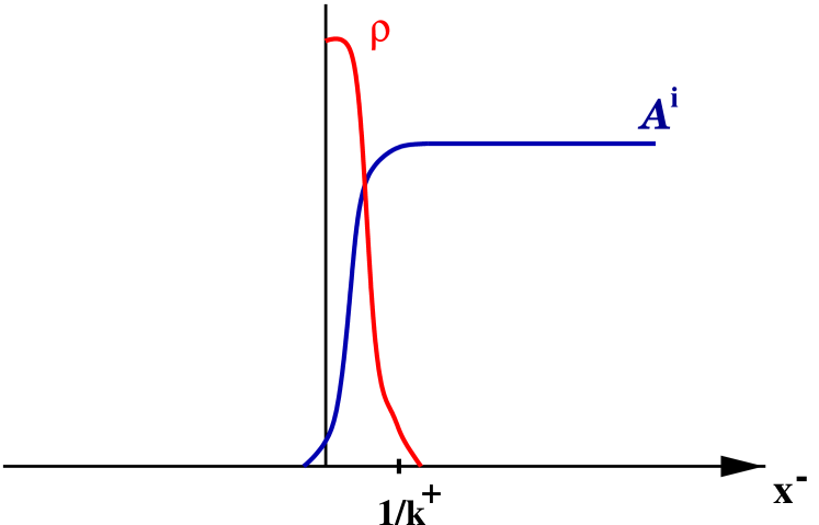
Up to this point, the longitudinal structure of the source has been arbitrary: the solutions written above hold for any function $\rho^{a}(x^{-})$. For what follows, however, it is useful to recall, from Sect. 2.1, that $\rho$ has is localized near $x^{-}=0$. More precisely, the quantum analysis in Sect. 3.4 will demonstrate that the classical source at the longitudinal scale $k^{+}$ has support at positive $x^{-}$, with $0\leq x^{-}\leq 1/k^{+}$. From eqs. (2.33)–(2.34), it is clear that this is also the longitudinal support of the “Coulomb field” $\alpha(\vec{x})$. Thus, integrals over $x^{-}$ as that in eq. (2.38) receive contributions only from $x^{-}$ in this limited range. The resulting longitudinal structure for the classical solution is illustrated in Fig. 12, and can be approximated as follows:

$${\cal A}^{i}(x^{-},x_{\perp}) \approx \theta(x^{-})\,\frac{i}{g}\,V(\partial^{i}V^{\dagger})\,\equiv\,\theta(x^{-}){\cal A}^{i}_{\infty}(x_{\perp}),$$ (2.43)

$${\cal F}^{+i}(\vec{x}) \equiv \partial^{+}{\cal A}^{i}\,\approx\,\delta(x^{-})\,{\cal A}^{i}_{\infty}(x_{\perp}).$$ (2.44)

It is here understood that the $\delta--$ and $\theta--$functions of $x^{-}$ are smeared over a distance $\Delta x^{-}\sim 1/k^{+}$. In the equations above, $V$ and $V^{\dagger}$ are the asymptotic values of the respective gauge rotations as $x^{-}\to\infty$ :

$$V^{\dagger}(x_{\perp})\,\equiv\,{\rm P}\exp\left\{ig\int_{-\infty}^{\infty}dz^{-}\,\alpha(z^{-},x_{\perp})\right\}.$$ (2.45)

In practice, $U(x^{-},x_{\perp})=V(x_{\perp})$ for any $x^{-}\gg 1/k^{+}$. Note that (2.45) is the same Wilson line as in the discussion of the eikonal approximation in Sect. 2.2.2 (compare to eq. (2.25) there). In the present context, the eikonal approximation is implicit in the special geometry of the colour source in eq. (2.1), which is created by fast moving particles.

Figure 12: The longitudinal structure of the colour source $\rho$ and of the classical field solution ${\cal A}^{i}$ for the effective theory at the scale $k^{+}\,$. As functions of $x^{-}$, $\alpha$ and ${\cal F}^{+i}$ are as localized as $\rho$.

2.4 The gluon distribution of the valence quarks

To compute observables in the effective theory, one still needs an expression for the weight function $W_{\tau}[\rho]$. Before discussing the general construction of $W_{\tau}[\rho]$ in Sect. 3, let us present a simple model for it, due to McLerran-Venugopalan (MV) [8], which takes into account the colour charge of the valence quarks alone. That is, it ignores the quantum evolution of the colour sources with $\tau$. This model is expected to work better for a large nucleus, with atomic number $A\gg 1\,$; indeed, this has many valence quarks ($A\times N_{c}$), and therefore as many colour sources, which can create a strong colour field already at moderate values of x, where the quantum evolution can be still neglected. In this model, $\tau$ is fixed, but one can study the strong field effects (in particular, gluon saturation) in the limit where $A$ is large. Besides, the MV model provides a reasonable initial condition for the quantum evolution towards small x, to be described later.

The main assumption of the MV model is that the $A\times N_{c}$ valence quarks can be treated as independent colour sources. This relies on confinement. Note first that confinement plays no role for the dynamics in the transverse plane: Indeed, we probe the nucleus with large transerse momenta $Q^{2}\gg\Lambda_{QCD}^{2}$, that is, over distance scales much shorter than those where confinement sets in. On the other hand, even at moderate values of x, we are still probing an integrated version of the hadron in the longitudinal direction, i.e., we measure all the “partons” (here, valence quarks) in a tube of transverse area $\Delta S_{\perp}\sim 1/Q^{2}$ and longitudinal extent $\Delta x^{-}\sim 1/{\rm x}P^{+}>1/P^{+}$. The number of valence quarks which are crossed by this tube,

$$\Delta N\approx n\,\Delta S_{\perp}\,=\,\Delta S_{\perp}\,\frac{AN_{c}}{\pi R^{2}_{A}}\sim A^{1/3}\,,$$ (2.46)

(with $n=$ the number of quarks per unit transverse area, $R$ the radius of a single nucleon, and $R_{A}=A^{1/3}R$ the radius of the nucleus) increases with $A$, but these quarks are confined within different nucleons, so they are uncorrelated. When the number of partons $\Delta N$ is large enough, the external probe “sees” them as a classical colour source with a random distribution over the transverse area. The total colour charge ${\cal Q}^{a}$ in the tube is the incoherent sum of the colour charges of the individual partons. Thus,

$$\langle{\cal Q}^{a}\rangle\,=\,0,\qquad\langle{\cal Q}^{a}{\cal Q}^{a}\rangle\,=\,g^{2}C_{f}\Delta N\,=\,\Delta S_{\perp}\,\frac{g^{2}C_{f}N_{c}A}{\pi R^{2}_{A}},$$ (2.47)

where we have used the fact that the colour charge squared of a single quark is $g^{2}t^{a}t^{a}=g^{2}C_{f}$. One can treat this charge as classical since, when $\Delta N$ is large enough, we can ignore commutators of charges:

$$\mid[{\cal Q}^{a},{\cal Q}^{b}]\mid\,=\,\mid if^{abc}{\cal Q}^{c}\mid\,\ll\,{\cal Q}^{2}\,.$$ (2.48)

In order to take the continuum limit (i.e., the limit where the transverse area $\Delta S_{\perp}$ of the tube is small), it is convenient to introduce the colour charge densities $\rho^{a}(x^{-},x_{\perp})$ (with the same meaning as in Sect. 2.1) and

$$\rho^{a}(x_{\perp})\equiv\int dx^{-}\rho^{a}(x^{-},x_{\perp})$$ (2.49)

(the colour charge per unit area in the transverse plane). Then,

$${\cal Q}^{a}\,=\,\int_{\Delta S_{\perp}}d^{2}x_{\perp}\,\rho^{a}(x_{\perp})\,=\,\int_{\Delta S_{\perp}}d^{2}x_{\perp}\int dx^{-}\,\rho^{a}(x^{-},x_{\perp}),$$ (2.50)

and eqs. (2.47) imply (recall that $C_{f}=(N_{c}^{2}-1)/2N_{c}$) :

$$\langle\rho_{a}(x_{\perp})\rho_{b}(y_{\perp})\rangle_{A} = \delta_{ab}\delta^{(2)}(x_{\perp}-y_{\perp})\,\mu_{A},\qquad\mu_{A}\equiv\frac{g^{2}A}{2\pi R^{2}_{A}}\,,$$

$$\langle\rho_{a}(x^{-},x_{\perp})\rho_{b}(y^{-},y_{\perp})\rangle_{A} = \delta_{ab}\delta^{(2)}(x_{\perp}-y_{\perp})\delta(x^{-}-y^{-})\,\lambda_{A}(x^{-}),$$

$$\int dx^{-}\,\lambda_{A}(x^{-}) = \mu_{A}\,.$$ (2.51)

Here, $\mu_{A}\sim A^{1/3}$ is the average colour charge squared of the valence quarks per unit transverse area and per colour, and $\lambda_{A}(x^{-})$ is the corresponding density per unit volume. The latter has some dependence upon $x^{-}$, whose precise form is, however, not important since the final formulae will involve only the integrated density $\mu_{A}$. There is no explicit dependence upon $x_{\perp}$ in $\mu_{A}$ or $\lambda_{A}(x^{-})$ since we assume transverse homogeneity within the nuclear disk of radius $R_{A}$. Finally, the correlations are local in $x^{-}$ since, as argued before, colour sources at different values of $x^{-}$ belong to different nucleons, so they are uncorrelated. All the higher-point, connected, correlation functions of $\rho_{a}(\vec{x})$ are assumed to vanish. The non-zero correlators (2.4) are generated by the following weight function [8] :

$$W_{A}[\rho]\,=\,{\cal N}{\rm exp}\left\{-\,{1\over 2}\,\int d^{3}x\frac{\rho_{a}(\vec{x})\rho_{a}(\vec{x})}{\lambda_{A}(x^{-})}\right\},$$ (2.52)

which is a Gaussian in $\rho_{a}$, with a local kernel. This is gauge-invariant, so the variable $\rho_{a}$ in this expression can be the colour source in any gauge. The integral over $x_{\perp}$ in eq. (2.52) is effectively cutoff at $R_{A}$. By using this weight function, we shall now compute the observables introduced in Sect.  2.2.

Consider first the gluon distribution in the low density regime, i.e., when the atomic number $A$ is not too high, so that the corresponding classical field is weak and can be computed in the linear approximation. By expanding the general solution (2.31) to linear order in $\rho$, or, equivalently, by directly solving the linearized version of eq. (2.1), one easily obtains:

$${\cal A}^{i}_{a}(k)\,\simeq\,-{k^{i}\over k^{+}+i\varepsilon}{\rho_{a}(k^{+},k_{\perp})\over k_{\perp}^{2}}\,,\qquad{\cal F}^{+i}_{a}(k)\,\simeq\,i{k^{i}\over k_{\perp}^{2}}\,{\rho_{a}(\vec{k})}\,,$$ (2.53)

which together with eq. (2.4) implies:

$$\langle{\cal F}^{i+}_{a}(\vec{k}){\cal F}^{i+}_{a}(-\vec{k})\rangle_{A}\simeq\frac{1}{k_{\perp}^{2}}\,\langle\rho_{a}(\vec{k})\rho_{a}(-\vec{k})\rangle_{A}\,=\,\pi R^{2}_{A}(N_{c}^{2}-1)\frac{\mu_{A}}{k_{\perp}^{2}}\,.\,\,\,\,$$ (2.54)

By inserting this approximation in eqs. (2.23) and (2.16), one obtains the following estimates for the gluon density and distribution function:

$${\cal N}_{A}(k_{\perp}) \simeq \frac{N_{c}^{2}-1}{4\pi^{3}}\,\frac{\mu_{A}}{k_{\perp}^{2}}\,,$$ (2.55)

$${\rm x}G({\rm x},Q^{2}) \simeq \frac{(N_{c}^{2}-1)R_{A}^{2}}{4\pi}\,\mu_{A}\int^{Q^{2}}_{\Lambda_{QCD}^{2}}\frac{dk_{\perp}^{2}}{k_{\perp}^{2}}\,=\,\frac{\alpha_{s}AN_{c}C_{f}}{\pi}\,\ln\frac{Q^{2}}{\Lambda_{QCD}^{2}}\,,$$

(with $\alpha_{s}=g^{2}/4\pi$). The integral over $k_{\perp}$ in the second line has a logarithmic infrared divergence which has been cut by hand at the scale $\Lambda_{QCD}$ since we know that, because of confinement, there cannot be gluon modes with transverse wavelengths larger than $1/\Lambda_{QCD}$ (see also Ref. [35]).

We recognize in eq. (2.55) the standard bremsstrahlung spectrum of soft “photons” radiated by fast moving charges [1]. In deriving this result, we have however neglected the non-Abelian nature of the radiated fields, i.e., the fact that they represent gluons, and not photons. This will be corrected in the next subsection.

2.5 Gluon saturation in a large nucleus

According to eq. (2.55), the gluon density in the transverse phase-space is proportional to $A^{1/3}$, and becomes arbitrarily large when $A$ increases. This is however an artifact of our previous approximations which have neglected the interactions among the radiated gluons, i.e., the non-linear effects in the classical field equations. To see this, one needs to recompute the gluon distribution by using the exact, non-linear solution for the classical field, as obtained in Sect. 2.3. This involves the following LC-gauge field-field correlator:

$$\langle{\cal F}^{+i}_{a}(\vec{x}){\cal F}^{+i}_{a}(\vec{y})\rangle_{A} = \Bigl{\langle}\Bigl{(}U_{ab}^{\dagger}\partial^{i}\alpha^{b}\Bigr{)}_{\vec{x}}\,\Bigl{(}U_{ac}^{\dagger}\partial^{i}\alpha^{c}\Bigr{)}_{\vec{y}}\Bigr{\rangle}_{A},$$ (2.56)

which, in view of the non-linear calculation, has been rewritten in terms of the classical field in the COV-gauge (cf. eq. (2.42)), where $\tilde{\cal F}^{+i}_{a}=-\partial^{i}\alpha_{a}$. To evaluate (2.56), one expands the Wilson lines in powers of $\alpha$ and then contracts the $\alpha$ fields in all the possible ways with the following propagator:

$$\langle\alpha_{a}(\vec{x})\alpha_{b}(\vec{y})\rangle_{A} = \delta_{ab}\delta(x^{-}-y^{-})\,\gamma_{A}(x^{-},x_{\perp}-y_{\perp}),$$

$$\gamma_{A}(x^{-},k_{\perp}) \equiv \frac{1}{k_{\perp}^{4}}\,\lambda_{A}(x^{-}).$$ (2.57)

We have used here $\tilde{\rho}^{a}(x^{-},k_{\perp})=k_{\perp}^{2}\alpha^{a}(x^{-},k_{\perp})$, cf. eq. (2.34), together with eq. (2.4) which holds in any gauge and, in particular, in the COV-gauge. The propagator (2.5) is very singular as $k_{\perp}\to 0$, but this turns out to be (almost) harmless for the considerations to follow.

The fact that the fields $\alpha$ are uncorrelated in $x^{-}$ greatly simplifies the calculation of the correlator (2.56). Indeed, this implies that the two COV-gauge electric fields $\partial^{i}\alpha_{b}(\vec{x})$ and $\partial^{i}\alpha_{c}(\vec{y})$ can be contracted only together, and not with the other fields $\alpha$ generated when expanding the Wilson lines. That is:

$$\Bigl{\langle}\Bigl{(}U_{ab}^{\dagger}\partial^{i}\alpha^{b}\Bigr{)}_{\vec{x}}\,\Bigl{(}U_{ac}^{\dagger}\partial^{i}\alpha^{c}\Bigr{)}_{\vec{y}}\Bigr{\rangle}=\left\langle\partial^{i}\alpha^{b}(\vec{x})\partial^{i}\alpha^{c}(\vec{y})\right\rangle\left\langle U_{ab}^{\dagger}(\vec{x})U_{ca}(\vec{y})\right\rangle$$

$$=\delta(x^{-}-y^{-})\langle{\rm Tr}\,U^{\dagger}(\vec{x})U(\vec{y})\rangle\big{(}-\nabla^{2}_{\perp}\gamma_{A}(x^{-},x_{\perp}-y_{\perp})\big{)},\quad$$ (2.58)

where we have used $U_{ac}^{\dagger}=U_{ca}$ in the adjoint representation. Eq. (2.5) can be proven as follows: i) By rotational symmetry, $\partial^{i}\alpha(\vec{x})$ cannot be contracted with a field $\alpha(z^{-},x_{\perp})$ resulting from the expansion of $U^{\dagger}(\vec{x})$; indeed:

$$\langle\alpha(z^{-},x_{\perp})\partial^{i}\alpha(x^{-},x_{\perp})\rangle\propto\partial^{i}\gamma_{A}(x^{-},r_{\perp})\Big{|}_{r_{\perp}=0}\propto\int{d^{2}k_{\perp}\over(2\pi)^{2}}\,\frac{-ik^{i}}{k_{\perp}^{2}}\,=\,0\,.$$

ii) Contractions of the type

$$\langle\alpha(z^{-},y_{\perp})\partial^{i}\alpha(x^{-},x_{\perp})\rangle\,\langle\alpha(u^{-},x_{\perp})\partial^{i}\alpha(y^{-},y_{\perp})\rangle\propto\delta(x^{-}-z^{-})\delta(u^{-}-y^{-})$$

are not allowed by the ordering of the Wilson lines in $x^{-}\,$: $\alpha(z^{-},y_{\perp})$ has been generated by expanding $U^{\dagger}(\vec{y})$, which requires $z^{-}<y^{-}$ (and similarly $u^{-}<x^{-}$). Then, the first contraction in (2.5) implies $x^{-}=z^{-}<y^{-}$, while the second one leads to the contradictory requirement $y^{-}=u^{-}<x^{-}$.

The allowed contractions in eq. (2.5) involve:

$$S_{A}(x^{-},x_{\perp}-y_{\perp})\,\equiv\,\frac{1}{N_{c}^{2}-1}\,\langle{\rm Tr}\,U^{\dagger}(x^{-},x_{\perp})U(x^{-},y_{\perp})\rangle_{A},$$ (2.59)

which is like the $S$-matrix element (2.26) for the dipole-hadron scattering, but now for a colour dipole in the adjoint representation (i.e., a dipole made of two gluons). This can be computed by expanding the Wilson lines, performing contractions with the help of eq. (2.5), and recognizing the result as the expansion of an ordinary exponential. One thus finds (see also Sect. 5.1 for a more rapid derivation):

$$S_{A}(x^{-},r_{\perp}) = {\rm exp}\Big{\{}-g^{2}N_{c}[\xi_{A}(x^{-},0_{\perp})-\xi_{A}(x^{-},r_{\perp})]\Big{\}},$$

$$\xi_{A}(x^{-},r_{\perp}) \equiv \int_{-\infty}^{x^{-}}dz^{-}\,\gamma_{A}(z^{-},r_{\perp}),$$ (2.60)

where the exponent can be easily understood: It arises as

$$\Big{\langle}gT^{a}(\alpha_{a}(\vec{x})-\alpha_{a}(\vec{y}))\,gT^{b}(\alpha_{b}(\vec{x})-\alpha_{b}(\vec{y}))\Big{\rangle}$$ (2.61)

where $igT^{a}(\alpha_{a}(\vec{x})-\alpha_{a}(\vec{y}))$ is the amplitude for the dipole scattering off the “Coulomb” field $\alpha_{a}$, to lowest order in this field (i.e., the amplitude for a single scattering). Then, (2.61) is the amplitude times the complex conjugate amplitude, that is, the cross section for such a single scattering. This appears as an exponent in eq. (2.5) since this equation resums multiple scatterings to all orders, and, in the eikonal approximation, the all-order result is simply the exponential of the lowest order result. Since, moreover, $\alpha_{a}$ is the field created by the colour sources in the hadron (here, the valence quarks), we deduce that eq. (2.5) describes the multiple scattering of the colour dipole off these colour sources.

If the field $\alpha_{a}$ is slowly varying over the transverse size $r_{\perp}=x_{\perp}-y_{\perp}$ of the dipole (“small dipole”), one can expand

$$gT^{a}(\alpha_{a}(\vec{x})-\alpha_{a}(\vec{y}))\approx-gT^{a}(x^{i}-y^{i})\partial^{i}\alpha_{a}(\vec{x})=gT^{a}(x^{i}-y^{i})\tilde{\cal F}^{+i}_{a}(\vec{x}),\quad$$ (2.62)

and then eq. (2.61) involves the correlator of two (COV-gauge) electric fields. This is indeed the case, at it can be seen by an analysis of the exponent in eq. (2.5) :

$$\xi_{A}(x^{-},0_{\perp})-\xi_{A}(x^{-},r_{\perp}) = \mu_{A}(x^{-})\int{d^{2}k_{\perp}\over(2\pi)^{2}}\,\frac{1}{k_{\perp}^{4}}\,\Bigl{[}1-{\rm e}^{ik_{\perp}\cdot r_{\perp}}\Bigr{]}\,,$$

$$\mu_{A}(x^{-}) \equiv \int_{-\infty}^{x^{-}}dz^{-}\lambda_{A}(z^{-}).$$ (2.63)

The above integral over $k_{\perp}$ is dominated by soft momenta, and has even a logarithmic divergence which reflects the lack of confinement in our model (see also [35]). Note, however, that the dominant, quadratic, infrared divergence $\sim\int(d^{2}k_{\perp}/k_{\perp}^{4})$, which would characterize the scattering of a coloured particle (a single gluon) off the hadronic field, has cancelled between the two components of the colourless dipole. The remaining, logarithmic, divergence can be cut off by hand, by introducing an infrared cutoff $\Lambda_{QCD}$. Then one can expand:

$$\int{d^{2}k_{\perp}\over(2\pi)^{2}}\frac{1-{\rm e}^{ik_{\perp}\cdot r_{\perp}}}{k_{\perp}^{4}}\simeq\int\limits^{1/r_{\perp}^{2}}{d^{2}k_{\perp}\over(2\pi)^{2}}\frac{1}{k_{\perp}^{4}}{(k_{\perp}\cdot r_{\perp})^{2}\over 2}\simeq{r_{\perp}^{2}\over 16\pi}\ln{1\over r_{\perp}^{2}\Lambda^{2}_{QCD}}\,.\,\,\,\,\,\,\,\,$$ (2.64)

(This is valid to leading logarithmic accuracy, since the terms neglected in this way are not enhanced by a large transverse logarithm.) We thus obtain:

$$S_{A}(x^{-},r_{\perp})\,\simeq\,{\rm exp}\left\{-\,\frac{\alpha_{s}N_{c}}{4}\,r_{\perp}^{2}\,\mu_{A}(x^{-})\,\ln{1\over r_{\perp}^{2}\Lambda^{2}_{QCD}}\right\},$$ (2.65)

which together with eq. (2.5) can be used to finally evaluate the gluon density (2.23). This requires a double Fourier transform (to $k^{+}$ and $k_{\perp}$), as shown in eq. (2.17). The presence of the $\delta$-function in eq. (2.5) makes the Fourier transform to $k^{+}$ trivial, and one gets:

$${\cal N}_{A}(k_{\perp})=\frac{N_{c}^{2}-1}{4\pi^{3}}\int d^{2}r_{\perp}{\rm e}^{-ik_{\perp}\cdot r_{\perp}}\int dx^{-}S_{A}(x^{-},r_{\perp})(-\nabla^{2}_{\perp}\gamma_{A}(x^{-},r_{\perp})),$$

where (cf. eqs. (2.5) and (2.5)) :

$$-\nabla^{2}_{\perp}\gamma_{A}(x^{-},r_{\perp})=\lambda_{A}(x^{-})\int{d^{2}p_{\perp}\over(2\pi)^{2}}\,\frac{{\rm e}^{ip_{\perp}\cdot x_{\perp}}}{p_{\perp}^{2}}=\frac{1}{4\pi}\ln{1\over r_{\perp}^{2}\Lambda^{2}_{QCD}}\,\frac{\partial\mu_{A}(x^{-})}{\partial x^{-}}.$$

The non-linear effects in eq. (2.5) are encoded in the quantity $S_{A}(x^{-},r_{\perp})$, which finds its origin in the gauge rotations in the r.h.s. of eq. (2.56). In fact, by replacing $S_{A}(x^{-},r_{\perp})\to 1$ in eq. (2.5), one would recover the linear approximation of eq. (2.55). To perform the integral over $x^{-}$ in eq. (2.5), we note that the quantity (2.5) is essentially the derivative w.r.t. $x^{-}$ of the exponent in $S_{A}(x^{-},r_{\perp})$, eq. (2.65). Therefore:

$${\cal N}_{A}(k_{\perp})=\frac{N_{c}^{2}-1}{4\pi^{4}}\!\int\!d^{2}r_{\perp}{\rm e}^{-ik_{\perp}\cdot r_{\perp}}\,\frac{1-{\rm exp}\Big{\{}-\frac{1}{4}\,r_{\perp}^{2}Q_{A}^{2}\ln{1\over r_{\perp}^{2}\Lambda^{2}_{QCD}}\Big{\}}}{\alpha_{s}N_{c}r_{\perp}^{2}}\,,\,\,$$ (2.68)

where

$$Q_{A}^{2}\,\equiv\,\alpha_{s}N_{c}\mu_{A}\,=\,\alpha_{s}N_{c}\int dx^{-}\lambda_{A}(x^{-})\,\sim\,A^{1/3}.$$ (2.69)

Eq. (2.68) is the complet result for the gluon density of a large nucleus in the MV model [33, 34]. To study its dependence upon $k_{\perp}$, one must still perform the Fourier transform, but the result can be easily anticipated:

i) At high momenta $k_{\perp}\!\gg\!Q_{A}$, the integral is dominated by small distances $r_{\perp}\!\ll\!1/Q_{A}$, and can be evaluated by expanding out the exponential. To lowest non-trivial order (which corresponds to the linear approximation), one obtains the bremsstrahlung spectrum of eq. (2.55):

$${\cal N}_{A}(k_{\perp})\,\propto\,\frac{1}{\alpha_{s}N_{c}}\,\frac{Q_{A}^{2}}{k_{\perp}^{2}}\,=\,\frac{\mu_{A}}{k_{\perp}^{2}}\qquad{\rm for}\quad k_{\perp}\gg Q_{A}.$$ (2.70)

ii) At small momenta, $k_{\perp}\!\ll\!Q_{A}$, the dominant contribution comes from large distances $r_{\perp}\!\gg\!1/Q_{A}$, where one can simply neglect the exponential in the numerator and recognize $1/r_{\perp}^{2}$ as the Fourier transform of $\ln k_{\perp}^{2}\,$:

$${\cal N}_{A}(k_{\perp})\,\approx\,\frac{N_{c}^{2}-1}{4\pi^{3}}\,\frac{1}{\alpha_{s}N_{c}}\ln\frac{Q_{A}^{2}}{k_{\perp}^{2}}\qquad{\rm for}\quad k_{\perp}\ll Q_{A}.$$ (2.71)

There are two fundamental differences between eqs. (2.70) and (2.71), which refer both to a saturation of the increase of the gluon density: either with $1/k_{\perp}^{2}$ (at fixed atomic number $A$), or with $A$ (at fixed transverse momentum $k_{\perp}$). In both cases, this saturation is only marginal : in the low–$k_{\perp}$ regime, eq. (2.71), the gluon density keeps increasing with $1/k_{\perp}^{2}$, and also with $A$, but this increase is only logarithmic, in contrast to the strong, power-like, increase $\propto(A^{1/3}/k_{\perp}^{2})$ in the high–$k_{\perp}$ regime, eq. (2.70).

Moreover, the gluon density at low $k_{\perp}$ is of order $1/{\alpha_{s}}\,$, which is the maximum density allowed by the repulsive interactions between the strong colour fields $\bar{A}^{i}=\sqrt{\langle A^{i}A^{i}\rangle}\sim 1/g$. When increasing the atomic number $A$, the new gluons are produced preponderently at large transverse momenta $\mathrel{\hbox to0.0pt{\raise 2.20013pt\hbox{$>$}\hss}{\lower 2.20013pt\hbox{$\sim$}}}Q_{A}$, where this repulsion is less important. This is illustrated in Fig. 13.

Figure 13: The gluon phase-space density ${\cal N}_{A}(k_{\perp})$ of a large nucleus (as described by the MV model) plotted as a function of $k_{\perp}$.

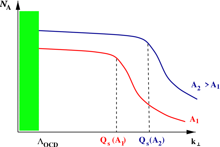
To be more precise, the true scale which separates between the two regimes (2.70) and (2.71) is not $Q_{A}$, but rather the saturation momentum $Q_{s}(A)$ which is the reciprocal of the distance $1/r_{\perp}$ where the exponent in eq. (2.68) becomes of order one. Thus, this is defined as the solution to the following equation:

$$Q_{s}^{2}(A)\,=\,{1\over 4}\,\alpha_{s}N_{c}\mu_{A}\,\ln{Q_{s}^{2}(A)\over\Lambda^{2}_{QCD}}\,.$$ (2.72)

To clarify its physical interpretation, note that, at short-distances $r_{\perp}\!\ll\!1/Q_{A}$,

$$\mu_{A}\,\ln{1\over r_{\perp}^{2}\Lambda^{2}_{QCD}}\,\propto\,\frac{{\rm x}G({\rm x},1/r_{\perp}^{2})}{(N^{2}_{c}-1)\pi R_{A}^{2}}\,$$ (2.73)

is the number of gluons (of each colour) having tranverse size $r_{\perp}$ per unit of transverse area (cf. eq. (2.55)). Since each such a gluon carries a colour charge squared $(gT^{a})(gT^{a})=g^{2}N_{c}$, we deduce that

$$\alpha_{s}N_{c}\,\mu_{A}\,\ln{1\over r_{\perp}^{2}\Lambda^{2}_{QCD}}$$ (2.74)

is the average colour charge squared of the gluons having tranverse size $r_{\perp}$ per unit area and per colour. Then, eq. (2.72) is the condition that the total colour charge squared within the area occupied by each gluon is of order one. This is the original criterion of saturation by Gribov, Levin and Ryskin [6], for which the MV model offers an explicit realization.

To conclude this discussion of the MV model, note that, in the previous computation, we have also obtained the $S$-matrix element $S_{A}(r_{\perp})$ for the dipole-hadron scattering (cf. Sect. 2.2.2). This is given by eq. (2.65) with $\mu_{A}(x^{-})\to\mu_{A}$ and $N_{c}=T^{a}T^{a}$ replaced in general by the colour Casimir $t^{a}t^{a}$ for the representation of interest (e.g., $C_{f}=(N^{2}_{c}-1)/2N_{c}$ for the fundamental representation). As discussed after eq. (2.61), this describes the multiple scattering of the colour dipole on the colour field in the hadron (here, the field of the valence quarks). According to eq. (2.65), one can distinguish, here too, between a short-distance and a large-distance regime, which moreover are separated by the same “saturation scale” as for the gluon distribution:

i) A small-size dipole $r_{\perp}\!\ll\!1/Q_{s}$ is only weakly interacting with the hadron:

$$1-S_{A}(r_{\perp})\,\approx\,\frac{1}{4}\,r_{\perp}^{2}Q_{A}^{2}\ln{1\over r_{\perp}^{2}\Lambda^{2}_{QCD}}\qquad{\rm for}\quad r_{\perp}\ll 1/Q_{s}(A),$$ (2.75)

a phenomenon usually referred to as “colour transparency”.

ii) A relatively large dipole, with $r_{\perp}\!\gg\!1/Q_{s}$, is strongly absorbed:

$$S_{A}(r_{\perp})\,\approx\,0\qquad{\rm for}\quad r_{\perp}\gg 1/Q_{s}(A),$$ (2.76)

a situation commonly referred to as the “black disk”, or “unitarity”, limit.

The remarkable fact that the critical dipole size is set by the saturation scale $Q_{s}$ can be understood as follows: A small dipole — small as compared to the typical variation scale of the external Coulomb field — couples to the associated electric field $\tilde{\cal F}^{+i}$ (cf. eq. (2.62)), so its cross-section for one scattering, eq. (2.61), is proportional to the number of gluons $\langle\tilde{\cal F}^{+i}\tilde{\cal F}^{+i}\rangle$ within the transverse area $r_{\perp}^{2}$ explored by the dipole. This is manifest on eq. (2.65), whose exponent is precisely the colour charge squared of the gluons within that area (cf. the remark after eq. (2.74)). At saturation, this charge becomes of order one, and the dipole is strongly interacting. The important lesson is that the unitarity limit (2.76) for the scattering of a small dipole on a high energy hadron is equivalent to gluon saturation in the hadron wavefunction [40, 9, 10, 45, 14].

3 Quantum evolution and
the Colour Glass Condensate

In this section, we show that the classical Yang-Mills theory described in Sect. 2 can be actually derived from QCD as an effective theory at small x. This requires integrating out quantum fluctuations in layers of $p^{+}$, which can be done with the help of a renormalization group equation (RGE) for the weight function $W_{\tau}[\rho]$. We shall not present all the calculations leading to this RGE; this would require heavy technical developments going far beyond the purpose of these lectures. (See Ref. [37] for more details.) Rather, we shall emphasize the general strategy of this construction and the physical picture behind it (that of the colour glass), together with those elements of the calculation which are important to understand the structure of the final equation.

3.1 The BFKL cascade

In Sect. 2.1, we have argued that the radiation of a soft gluon by a fast parton via the tree-level graph shown in Fig. 10.a can be described as a classical process with a colour source whose structure is largerly fixed by the kinematics. Our main goal in this section will be to show that this picture is not spoilt by quantum corrections. We start by showing that the dominant quantum corrections, those which will be resummed in what follows, preserve indeed the separation of scales which lies at the basis of the effective theory developed in Sect. 2.

Consider first the lowest-order radiative correction to the tree-level graph in Fig. 10.a, namely, the emission of one additional (quantum) gluon, as shown in Fig. 14.a. At the same level of accuracy, one should include also the vertex and self-energy corrections illustrated in Fig. 14.b, c. This will be done in the complete calculation presented in Sect. 3.4. But in order to get a simple order-of-magnitude estimate for the quantum corrections — which is our purpose in this subsection — it is enough to consider the radiative process in Fig. 14.a.

Figure 14: Lowest-order quantum corrections to the emission of a soft gluon by a fast parton: a) a real-gluon emission; b) a vertex correction; c) a self-energy correction.

The probability for the emission of a quantum gluon with longitudinal momentum $p_{1}^{+}$ in the range $p^{+}>p_{1}^{+}>k^{+}$ is

$$\Delta P\,\propto\,\frac{\alpha_{s}N_{c}}{\pi}\int_{k^{+}}^{p^{+}}\,\frac{dp_{1}^{+}}{p_{1}^{+}}\,=\,\frac{\alpha_{s}N_{c}}{\pi}\,\ln\,\frac{p^{+}}{k^{+}}\,\sim\,\alpha_{s}\ln\frac{1}{\rm x}\,.$$ (3.1)

This becomes large when the available interval of rapidity $\Delta\tau=\ln(1/{\rm x})$ is large. This is the typical kind of quantum correction that we would like to resum here. A calculation which includes effects of order $(\alpha_{s}\ln(1/{\rm x}))^{n}$ to all orders in $n$ is said to be valid to “leading logarithmic accuracy” (LLA).

The typical contributions to the logarithmic integration in eq. (3.1) come from modes with momenta $p_{1}^{+}$ deeply inside the strip: $p^{+}\gg p_{1}^{+}\gg k^{+}$. Thus, in Fig. 14.a, the soft final gluon with momentum $k^{+}$ is emitted typically from a relatively fast gluon, with momentum $p_{1}^{+}\gg k^{+}$. This latter gluon can therefore be seen as a component of the effective colour source at the soft scale $k^{+}$. In other terms, one can visualise the combined effect of the tree-level process, Fig. 10.a, and the first-order radiative correction, Fig. 14.a, as the generation of a modified colour source at the scale $k^{+}$, which receives contributions only from the modes with longitudinal momenta much larger than $k^{+}$. This is illustrated in Fig. 15.

Figure 15: Effective colour source after including the lowest-order radiative correction.

Clearly, when x is small enough, $\ln(1/{\rm x})\sim 1/\alpha_{s}$, the “correction” (3.1) becomes of ${\cal O}(1)$, and it is highly probable that more gluons will be emitted along the way. This gives birth to the gluon cascade depicted in Fig. 10.b, whose dominant contribution, for a fixed number of “rungs” $N$, is of order $(\alpha_{s}\ln(1/x))^{N}$, and comes from the kinematical domain where the longitudinal momenta are strongly ordered:

$$p^{+}\equiv p_{0}^{+}\,\gg\,p_{1}^{+}\,\gg\,p_{2}^{+}\,\gg\,\cdots\,\gg\,p_{N}^{+}\equiv k^{+}.$$ (3.2)

(Other momentum orderings give contributions which are suppressed by, at least, one factor of $1/\ln(1/{\rm x})$, and thus can be neglected to LLA.) With this ordering, this is the famous BFKL cascade, that we would like to include in our effective source. This should be possible since the hierarchy of scales in eq. (3.2) is indeed consistent with the kinematical assumptions in Sect. 2.

Note first that, the strong ordering (3.2) in longitudinal momenta implies a corresponding ordering in the lifetimes of the emitted gluons (cf. eq. (2.2)):

$$\Delta x^{+}_{0}\,\gg\,\Delta x^{+}_{1}\gg\,\Delta x^{+}_{2}\,\gg\,\cdots\,\gg\,\Delta x^{+}_{N}.$$ (3.3)

Because of this, any newly emitted gluon lives too shortly to notice the dynamics of the gluons above it. This is true in particular for the last emitted gluon, with momentum $k^{+}$, which “sees” the $N$ previous gluons in the cascade as a frozen colour charge distribution, with an average colour charge ${\cal Q}\equiv\sqrt{\langle{\cal Q}_{a}{\cal Q}_{a}\rangle}\sim N\/$. Thus, this $(N+1)$th gluon is emitted coherently off the colour charge fluctuations of the $N$ previous ones, with a differential probability (compare to eq. (3.1)) :

$$dP_{N}\,\propto\,\frac{\alpha_{s}N_{c}}{\pi}\,N(\tau)\,d\tau.$$ (3.4)

When increasing the rapidity by one more step, $\tau\to\tau+d\tau$, the number of radiated gluons changes according to

$$N(\tau+d\tau)=(1+N(\tau))dP_{N}+N(\tau)(1-dP_{N}),$$ (3.5)

which together with eq. (3.4) implies (with $\bar{\alpha}_{s}\equiv\alpha_{s}N_{c}/\pi$)

$${\rm x}G({\rm x},Q^{2})\,\equiv\,{dN\over d\tau}\,\sim\,C\alpha_{s}{\rm e}^{\kappa\bar{\alpha}_{s}\tau}.$$ (3.6)

Thus, the gluon distribution grows exponentially with $\tau=\ln(1/{\rm x})$. A more refined treatment, using the BFKL equation, gives $\kappa=4\ln 2$, and shows that the prefactor $C$ in the r.h.s. of eq. (3.6) has actually a weak dependence on $\tau\,$: $C\propto(\alpha_{s}\tau)^{-1/2}$ [3, 4].

Thus, the BFKL picture is that of an unstable growth of the colour charge fluctuations as x becomes smaller and smaller. However, this evolution assumes the radiated gluons to behave as free particles, so it ceases to be valid at very low ${\rm x}$, where the gluon density becomes so large that their mutual interactions cannot be neglected anylonger. This happens, typically, when the interaction probability for the radiated gluons becomes of order one, cf. eq. (1.12), which is also the criterion for the saturation effects to be important (compare in this respect eq. (1.12) and eqs. (2.72)–(2.73)). Thus one cannot study saturation consistently without including non-linear effects in the quantum evolution. It is our main objective in what follows to explain how to do that.

3.2 The quantum effective theory

To the accuracy of interest, quantum corrections can be incorporated in the effective theory by renormalizing the source $\rho_{a}$ and its correlation functions (i.e., the weight function $W_{\tau}[\rho]$). The argument proceeds by induction: We assume the effective theory to exist at some scale $\Lambda^{+}$ and show that it can be extended at the lower scale $b\Lambda^{+}\ll\Lambda^{+}$. Specifically:

I) We assume that a quantum effective theory exists at some original scale $\Lambda^{+}$ with $\Lambda^{+}\ll P^{+}$. That is, we assume that the fast quantum modes with momenta $p^{+}\gg\Lambda^{+}$ can be replaced, as far as their effects on the correlation functions at the scale $\Lambda^{+}$ are concerned, by a classical random source $\rho_{a}$ with weight function $W_{\Lambda^{+}}[\rho]$. (We shall eventually convert $\Lambda^{+}$ into the rapidity $\tau$ by using $\tau=\ln(P^{+}/\Lambda^{+})$.) On the other hand, the soft gluons, with momenta $p^{+}<\Lambda^{+}$, are still explicitely present in the theory, as quantum gauge fields. Thus, this effective theory includes both the classical field ${\cal A}^{i}[\rho]$ generated by $\rho$, and the soft quantum gluons.

Within this theory, the correlation functions of the soft ($k^{+}\leq\Lambda^{+}$) fields are obtained as (e.g., for the 2-point function)

$$\langle{\rm T}A^{\mu}(x)A^{\nu}(y)\rangle=\int{\cal D}\rho\,W_{\Lambda^{+}}[\rho]\left\{\frac{\int^{\Lambda^{+}}{\cal D}A\,\delta(A^{+})\,A^{\mu}(x)A^{\nu}(y)\,{\rm e}^{\,iS[A,\,\rho]}}{\int^{\Lambda^{+}}{\cal D}A\,\delta(A^{+})\,\,{\rm e}^{\,iS[A,\,\rho]}}\right\},$$

where T stays for time ordering (i.e. ordering in $x^{+}$). This is written in the LC-gauge $A^{+}_{a}=0$, and involves two functional integrals:

a) a quantum path integral over the soft gluon fields $A^{\mu}$ at fixed $\rho$:

$$\langle{\rm T}A^{\mu}(x)A^{\nu}(y)\rangle_{\rho}\,=\,\frac{\int^{\Lambda^{+}}{\cal D}A\,\delta(A^{+})\,A^{\mu}(x)A^{\nu}(y)\,{\rm e}^{\,iS[A,\,\rho]}}{\int^{\Lambda^{+}}{\cal D}A\,\delta(A^{+})\,\,{\rm e}^{\,iS[A,\,\rho]}},$$ (3.8)

b) a classical average over $\rho$, like in eq. (2.6) :

$$\langle{\rm T}A^{\mu}(x)A^{\nu}(y)\rangle\,=\,\int{\cal D}\rho\,W_{\Lambda^{+}}[\rho]\,\langle{\rm T}A^{\mu}(x)A^{\nu}(y)\rangle_{\rho}\,.$$ (3.9)

The upper script “$\Lambda^{+}$” on the quantum path integral is to recall the restriction to soft ($|p^{+}|<\Lambda^{+}$) longitudinal momenta. The action $S[A,\,\rho]$ is chosen such as to generate the classical field equations (2.1) in the saddle point approximation $\delta S/\delta A^{\mu}=0$. This requirement, together with gauge symmetry and the eikonal approximation, single out the following action [36] :

$$S[A,\rho]=-\int d^{4}x\,{1\over 4}\,F_{\mu\nu}^{a}F^{\mu\nu}_{a}+{i\over{gN_{c}}}\int d^{3}\vec{x}\,{\rm Tr}\,\Bigl{\{}\rho(\vec{x})\,W[A^{-}](\vec{x})\Bigr{\}},\,\,\,$$ (3.10)

where $W[A^{-}]$ is a Wilson line in the temporal direction:

$$W[A^{-}](\vec{x})\,=\,{\rm T}\,\exp\left\{\,ig\int dx^{+}A^{-}(x)\right\}.$$ (3.11)

With this action, the condition $\delta S/\delta A^{\mu}=0$ implies indeed eq. (2.1) for field configurations having $A^{-}_{a}=0$. Thus, the classical solution ${\cal A}^{\mu}_{a}=\delta^{\mu i}{\cal A}^{i}_{a}[\rho]$ found in Sect. 2.3 is the tree-level field in the present quantum theory.

As long as we are interested in correlation functions at the scale $\Lambda^{+}$, or slightly below it, we can satisfy ourselves with this classical (or saddle point) approximation. That is, to the accuracy to which holds the effective theory in eq. (3.2), the gluon correlations at the scale $\Lambda^{+}$ can be computed from the classical field solution, as in eq. (2.6). But quantum corrections become important when we consider correlations at a much softer scale $k^{+}\ll\Lambda^{+}$, such that $\alpha_{s}\ln(\Lambda^{+}/k^{+})\sim 1$.

II) Within the quantum effective theory, we integrate out the semi-fast quantum fluctuations, i.e., the fields with longitudinal momenta inside the strip:

$$\,\,b\Lambda^{+}\,\,\ll\,\,|p^{+}|\,\,\ll\,\,\Lambda^{+}\,,\quad{\rm with}\quad b\ll 1\quad{\rm and}\quad\alpha_{s}\ln(1/b)<1.$$ (3.12)

This generates quantum corrections to the correlation functions at the softer scale $b\Lambda^{+}$, which can be computed by decomposing the total gluon field as follows:

$$A^{\mu}_{c}\,=\,{\cal A}^{\mu}_{c}[\rho]+a^{\mu}_{c}+\delta A^{\mu}_{c}.$$ (3.13)

Here, ${\cal A}^{\mu}_{c}$ is the tree-level field, $a^{\mu}_{c}$ are the semi-fast fluctuations to be integrated out, and $\delta A^{\mu}_{c}$ are the soft modes with momenta $|p^{+}|\leq b\Lambda^{+}$ whose correlations receive quantum corrections from the semi-fast gluons.

These induced correlations must be computed to leading order in $\alpha_{s}\ln(1/b)$ (LLA), but to all orders in the classical fields ${\cal A}^{i}[\rho]$ (since we expect ${\cal A}^{i}\sim 1/g$ at saturation). This amounts to an one-loop calculation, but with the exact background field propagator $\langle a^{\mu}(x)a^{\nu}(y)\rangle_{\rho}$ of the semi-fast gluons. For instance, the quantum corrections to the 2-point function read schematically:

$$\big{\langle}({\cal A}^{i}[\rho]+\delta A^{i})({\cal A}^{j}[\rho]+\delta A^{j})\big{\rangle}_{\rho}\,-\,{\cal A}^{i}[\rho]{\cal A}^{j}[\rho]\,=\,$$

$$=\,{\cal A}^{i}[\rho]\langle\delta A^{j}\rangle_{\rho}+\langle\delta A^{i}\rangle_{\rho}\,{\cal A}^{j}[\rho]+\langle\delta A^{i}\delta A^{j}\rangle_{\rho}$$ (3.14)

where the brackets $\langle\cdots\rangle_{\rho}$ stand for the quantum average over the semi-fast fields in the background of $\rho\,$; this average is defined as in eq. (3.8), but with the functional integral now restricted to the fields $a^{\mu}_{c}$. The purpose of the quantum calculation is to provide explicit expressions for the 1-point function $\langle\delta A^{i}\rangle_{\rho}$ and the 2-point function $\langle\delta A^{i}\delta A^{j}\rangle_{\rho}$ as functionals of $\rho$ (to the indicated accuracy). Once these expressions are known, the 2-point function $\langle A^{i}(x)A^{j}(y)\rangle$ at the scale $b\Lambda^{+}$ can be finally computed as:

$$\langle A^{i}A^{j}\rangle\,=\,\Big{\langle}\big{\langle}({\cal A}^{i}[\rho]+\delta A^{i})({\cal A}^{j}[\rho]+\delta A^{j})\big{\rangle}_{\rho}\,\Big{\rangle}_{W_{\Lambda}},$$ (3.15)

where the external brackets $\langle\cdots\rangle_{W_{\Lambda}}$ denote the classical average over $\rho$ with weight function $W_{\Lambda}[\rho]$, as in eq. (3.9).

III) We finally show that the induced correlations can be absorbed into a functional change $W_{\Lambda^{+}}[\rho]\to W_{b\Lambda^{+}}[\rho]$ in the weight function for $\rho$. That is, the result (3.15) of the classical+quantum calculation in the effective theory at the scale $\Lambda^{+}$ can be reproduced by a purely classical calculation, but with a modified weight function $W_{b\Lambda^{+}}[\rho]$, corresponding to a new effective theory:

$$\Big{\langle}\langle({\cal A}^{i}[\rho]+\delta A^{i})({\cal A}^{j}[\rho]+\delta A^{j})\rangle_{\rho}\,\Big{\rangle}_{W_{\Lambda}}\,=\,\big{\langle}{\cal A}^{i}[\rho]{\cal A}^{i}[\rho]\big{\rangle}_{W_{b\Lambda}},$$ (3.16)

where the average in the r.h.s. is defined as in eq. (2.6), or (3.9), but with weight function $W_{b\Lambda^{+}}[\rho]$. This demonstrates the existence of the effective theory at the softer scale $b\Lambda^{+}$.

Since $\Delta W\equiv W_{b\Lambda^{+}}-W_{\Lambda^{+}}\propto\alpha_{s}\ln(1/b)$, the evolution of the weight function is best written in terms of rapidity: $W_{\tau+\Delta\tau}-W_{\tau}=-\Delta\tau HW_{\tau}$, where $\tau=\ln(P^{+}/\Lambda^{+})$, $\Delta\tau=\ln(1/b)$, and $H\equiv H[\rho,{\delta\over\delta\rho}]$ is a functional differential operator acting on $W_{\tau}$ (generally, a non-linear functional of $\rho$). In the limit $\Delta\tau\to 0$, this gives a renormalization group equation (RGE) describing the flow of the weight function with $\tau$ [33, 36] :

$${\partial W_{\tau}[\rho]\over{\partial\tau}}\,=\,-H\Big{[}\rho\,,{\delta\over\delta\rho}\Big{]}W_{\tau}[\rho]\,.$$ (3.17)

By integrating this equation with initial conditions at $\tau\ll 1$ (i.e., at $\Lambda^{+}\sim P^{+}$), one can obtain the weight function at the rapidity $\tau$ of interest. The initial conditions are not really perturbative, but one can rely on some non-perturbative model, like the MV model discussed in Sects. 2.4–2.5.

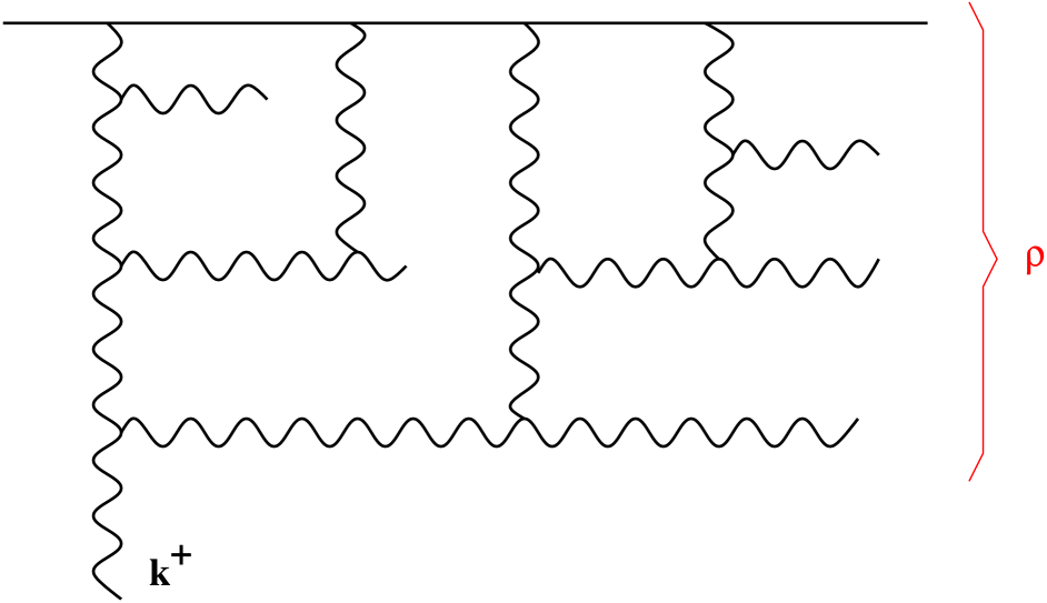
A key ingredient in this approach, which makes the difference w.r.t. the BFKL equation, are the non-linear effects encoded in the background field calculation. Recall that $\rho$, and therefore the classical fields ${\cal A}^{i}[\rho]$, are random variables whose correlators (2.6) reproduce the gluon density and, more generally, the $n$-point correlation functions of the gluon fields at the scale $\Lambda^{+}$. Thus by computing quantum corrections in the presence of these background fields, and then averaging over the latter, one is effectively studying quantum evolution in a medium with high gluon density. After each step in this evolution, the properties of the medium (i.e., the correlators of $\rho$) are updated, by including the latest quantum corrections. In terms of Feynman graphs of the ordinary perturbation theory, this corresponds to a complicated resummation of diagrams describing the interactions between the gluons radiated in different parton cascades and at different rapidities. A typical such a diagram is shown in Fig. 16. At low density, where the non-linear effects can be neglected, eq. (3.17) correctly reproduces the BFKL equation [36], as it should (see Sect. 3.5 below).

Figure 16: A typical Feynman diagram that is implicitely resummed in the quantum evolution of the effective theory.

3.3 The Colour Glass Condensate

Note the special form of the average in eq. (3.2). This is not the same as :

$$\frac{\int{\cal D}\rho\,\,W_{\Lambda}[\rho]\,\int^{\Lambda}{\cal D}A\,A^{\mu}(x)A^{\nu}(y)\,\,{\rm e}^{\,iS[A,\,\rho]}}{\int{\cal D}\rho\,\,W_{\Lambda}[\rho]\,\int^{\Lambda}{\cal D}A\,\,{\rm e}^{\,iS[A,\,\rho]}}\,.$$ (3.18)

In eq. (3.18), both the colour source $\rho_{a}$ and the gauge fields $A^{\mu}_{a}$ are dynamical variables that are summed over on the same footing. They are free to take on values which extremize the total “effective action” :

$$S_{eff}[A,\,\rho]\,=\,S[A,\,\rho]\,-\,i\ln W_{\Lambda}[\rho].$$ (3.19)

By contrast, in eq. (3.2), the average over $A^{\mu}$ is taken at fixed $\rho$ : the gauge fields can vary in response to $\rho$, but $\rho$ cannot vary in response to the gauge fields. That is, $\rho$ is not a dynamical variable, but rather an “external” source. Giving a colour charge distribution $\rho_{a}(\vec{x})$ specifies a medium in which propagate the quantum gluons. But this medium is, by itself, random, so after performing the quantum analysis at fixed $\rho$, one must also perform an average over $\rho$. The reason for treating $\rho$ and $A^{\mu}$ differently lies is the separation of scales in the problem: the changes in $\rho$ happens on time scales much larger than the lifetime of the soft gluons. This situation is typical for amorphous materials called “glasses”.

The prototype of such systems is a “spin glass” [43], that is, a collection of magnetic impurities (the “spins”) which are randomly distributed in a non-magnetic metal host. For instance, one can take the spins to sit on a regular lattice with lattice sites $i,j,\dots$, and interaction Hamiltonian

$$H_{J}[S]\,=\,-\sum_{<i,j>}J_{ij}S_{i}S_{j},$$ (3.20)

(the sum runs over all pairs $<i,j>$, and the spins $S_{i}$ are allowed to take two values, $+1$ or $-1$), but let their interactions (the “link variables” $J_{ij}$) to be random, with a Gaussian probability distribution, for simplicity:

$$dP[J]\,=\,\prod_{<i,j>}dJ_{ij}P(J_{ij}),\qquad P(J_{ij})\,=\,\frac{1}{\sqrt{2\pi\Delta_{ij}}}\,{\rm e}^{-\frac{J_{ij}^{2}}{2\Delta_{ij}}}.$$ (3.21)

Physically, this corresponds to the fact that the modifications in $J_{ij}$ occur on time scales much larger than the time scales characterizing the dynamics of the spins (e.g., their thermalization when the system is brought in contact with a thermal bath). In practice, the $J_{ij}$’s are frozen into their fixed values by rapid cooling when the sample is prepared. This kind or rapid cooling is called “quenching”, and one says that the $J_{ij}$’s are “quenched variables”, as opposed to the “dynamical variables”, the spins $S_{i}$. This procedure selects random values for the $J_{ij}$’s, with the probability distribution (3.21).

Thus, the spins thermalize for a given set of “quenched variables”, and for each such a set one can compute the thermal partition function and the free energy:

$$Z[J]\,=\,\sum_{\{S\}}\,{\rm e}^{-\beta H_{J}[S]},\qquad F[J]\,=\,-T\ln Z[J].$$ (3.22)

But the $J_{ij}$’s are themselves random, so the experimentally relevant quantity is the following average

$$F\,=\,\langle F[J]\rangle\,\equiv\,\int dP[J]\,F[J]\,=\,-T\int dP[J]\,\ln Z[J].$$ (3.23)

Note that it is $\ln Z[J]$, not $Z[J]$ itself, which should be averaged (“quenched average”). Similarly, (connected) correlation functions are generated by the free energy in the presence of a site-dependent external magnetic field:

$$\langle S_{i}S_{j}\rangle\,-\,\langle S_{i}\rangle\langle S_{j}\rangle\,=\,T^{2}\int dP[J]\,\frac{\partial^{2}\ln Z[J,h]}{\partial h_{i}\partial h_{j}}\,,$$ (3.24)

with $\ln Z[J,h]$ defined as in eq. (3.22), but with $H_{J}[S]\to H_{J}[S]-\sum_{i}h_{i}S_{i}$.

Eqs. (3.23)–(3.24) are the analogs of eq. (3.2) for the problem at hand: the colour source $\rho_{a}$ is our “quenched variable”, and the quantum average over the fields $A^{\mu}$ at fixed $\rho$, eq. (3.8), corresponds to the thermal average at fixed $J_{ij}$’s, eq. (3.22). As in eq. (3.23), it is $\ln Z$, and not $Z$, which is effectively averaged in eq. (3.2) (the average of $Z$ would rather corresponds to eq. (3.18)). In fact, the connected correlation functions of the soft gluons in the effective theory are obtained from the following generating functional:

$${F}[j^{\mu}_{a}]\,=\,\int{\cal D}\rho\,\,W_{\Lambda}[\rho]\,\,\ln\left(\int^{\Lambda}{\cal D}A\,\delta(A^{+})\,\,{\rm e}^{\,iS[A,\,\rho]-i\int j\cdot A}\right),$$ (3.25)

which is the analog of eq. (3.23) with $\ln Z[J]\to\ln Z[J,h]$. (The external current $j^{\mu}_{a}$ in (3.25) is just a device to generate Green’s functions via differentiations, and should not be confused with the physical source $\rho_{a}$.)

We are thus naturally led to interprete the small-x component of the hadron wavefunction as a glass, with the colour charge density playing the role of the spin for spin glasses. Thus, this is a colour glass. Unlike what happens for spin glasses, which may have a non-zero value for the average magnetization $\langle S_{i}\rangle$ (at least locally, i.e., at a given site), the average colour charge must be zero,

$$\langle\rho_{a}(\vec{x})\rangle\,=\,0\quad{\rm at\,\,any\,\,}\vec{x},$$ (3.26)

by gauge symmetry. In practice, this is insured by the fact that we sum over all the possible configurations of $\rho_{a}(\vec{x})$ with a gauge-invariant weight function. Let us however examine a particular configuration $\rho_{a}(\vec{x})$ from this ensemble. We now argue that, at sufficiently small x (or large atomic number $A$), this configuration describes typically a Bose condensate.

This applies to the saturated modes, i.e., the modes with transverse momenta $\Lambda_{QCD}\ll k_{\perp}\ll Q_{s}(\tau)$ and longitudinal momenta $k^{+}={\rm x}P^{+}\ll P^{+}$. As argued in Sect. 2.5, these modes are characterized by a high gluon number density in the transverse phase-space, ${\cal N}_{\tau}(k_{\perp})\sim 1/\alpha_{s}$. (This prediction of the classical MV model remains valid after including the quantum evolution, as we shall see in Sect. 5.4 below.) Microscopically, these modes correspond to bosonic states with large occupation numbers $\sim 1/\alpha_{s}$. Each such a state is a Bose condensate.

More precisely, the general definition of a Bose condensate is that of a quantum state in which the Fock space annihilation operator $a^{i}_{c}(\vec{k})$ (cf. eq. (2.13)), or, equivalently, the field operator $A^{i}_{c}(x)$, takes on a non-zero expectation value. This situation may be characterized as the spontaneous generation of a classical field. Of course, this cannot happen for gluons in the vacuum, as it would violate gauge symmetry. And, in an absolute sense, this cannot happen in a hadron neither, since the average colour charge vanishes there too (cf. eq. (3.26)), and therefore so does the associated classical field: $\langle{\cal A}^{i}_{c}[\rho]\rangle=0$. But in the hadron there are colour sources, and, as argued before, they can be even treated as a classical charge distribution which is frozen during the short lifetime of the small-x gluons. Thus, over such a short time scale (short as compared to the typical time scale for changes in the colour distribution), one effectively has a non-trivial classical field ${\cal A}^{i}_{c}[\rho]$. At saturation, this field is typically strong (cf. eqs. (2.68) and (2.44)) :

$$\Bigl{\langle}{\cal A}^{ia}_{\infty}(x_{\perp})\,{\cal A}^{ia}_{\infty}(y_{\perp})\Bigr{\rangle} \approx \frac{N_{c}^{2}-1}{\pi N_{c}}\frac{1-{\rm e}^{-r_{\perp}^{2}Q_{s}^{2}}}{\alpha_{s}r_{\perp}^{2}}\,,$$ (3.27)

$$\bar{\cal A}^{i}\,\sim\,\sqrt{{\langle{\cal A}^{i}_{\infty}{\cal A}^{i}_{\infty}\rangle}} \sim \frac{1}{\sqrt{\alpha_{s}r_{\perp}^{2}}}\qquad{\rm for}\,\,\,\,r_{\perp}\gg 1/Q_{s}\,,$$ (3.28)

and its typical amplitude (3.28) at large $r_{\perp}$ is even independent of the actual strength $\bar{\rho}\sim\sqrt{\langle\rho_{a}\rho_{a}\rangle}\sim Q_{s}$ of the colour source. This can be thus characterized as a Bose condensate.

We thus see that it is the same fundamental separation in time scales which allows us to speak about both the colour glass and the Bose condensate, although these two concepts seem at a first sight contradictory: the notion of a “glass” makes explicit reference to the average over $\rho$, while the “condensate” rather refers to a specific realization of $\rho$, before averaging.

3.4 The renormalization group equation

As explained in Sect. 3.2, the quantum evolution of the effective theory is obtained by matching correlations computed in two ways: (a) via a classical+quantum calculation in the effective theory at the scale $\Lambda^{+}$, and (b) via a purely classical calculation within the effective theory at the scale $b\Lambda^{+}$. The quantum corrections that are included in this way are those generated by the coupling between the “semi-fast” gluons with $p^{+}$ momenta in the strip (3.12) and the “soft” gluons $\delta A^{\mu}_{c}$ with momenta $|p^{+}|\leq b\Lambda^{+}$. To the accuracy of interest, it is sufficient to consider the eikonal coupling $\delta A^{-}_{a}\delta\hat{\rho}_{a}$ to the plus component $\delta\hat{J}^{+}_{a}\equiv\delta\hat{\rho}_{a}$ of the colour current of the semi-fast gluons. Indeed, these gluons are relatively fast moving in the $x^{+}$ direction, so $\delta\hat{\rho}_{a}$ is the large component of their current.

The results of the matching can be summarized as follows:

i) To ${\cal O}(\alpha_{s}\ln(1/b))$, the induced correlations of the transverse fields $A^{i}_{a}$ (see eq. (3.2) for an example) can be all related to the following 1-point and 2-point functions of $\delta\hat{\rho}$ (with $\Delta\tau=\ln(1/b)$) :

$$\sigma_{a}({x}_{\perp}) \equiv \frac{1}{\Delta\tau}\int dx^{-}\,\langle\delta\hat{\rho}_{a}(x)\rangle_{\rho}\,,$$ (3.29)

$$\chi_{ab}(x_{\perp},y_{\perp}) \equiv \frac{1}{\Delta\tau}\int dx^{-}\int dy^{-}\,\langle\delta\hat{\rho}_{a}(x^{+},\vec{x})\,\delta\hat{\rho}_{b}(x^{+},\vec{y})\rangle_{\rho}\,,$$ (3.30)

where, as in eq. (3.2), $\langle\cdots\rangle_{\rho}$ denotes the average over semi-fast quantum fluctuations in the background of the tree-level source $\rho$.

Thus the quantum evolution consists in adding new correlations $\sigma$ and $\chi$ to $\rho$.

ii) These new correlations can be included in the weight function $W_{\tau}[\rho]$ by allowing this to evolve with $\tau$ according to the following RGE [36, 37] :

$${\partial W_{\tau}[\rho]\over{\partial\tau}}\,=\,{1\over 2}{\delta^{2}\over{\delta\rho_{\tau}^{a}(x_{\perp})\delta\rho_{\tau}^{b}(y_{\perp})}}[W_{\tau}\chi_{xy}^{ab}]-{\delta\over{\delta\rho_{\tau}^{a}(x_{\perp})}}[W_{\tau}\sigma_{x}^{a}]\,.$$ (3.31)

We use here compact notations where $\sigma_{x}^{a}\equiv\sigma_{a}(x_{\perp})$, $\chi_{xy}^{ab}\equiv\chi_{ab}(x_{\perp},y_{\perp})$, and repeated colour indices (and coordinates) are understood to be summed (integrated) over. The notation $\rho_{\tau}^{a}(x_{\perp})$ will be explained later (see eq. (3.4.2)).

A complete proof of the statements above would require the lengthy analysis of Refs. [37]. But assuming them to be true, it is easy to understand the general structure of the RGE (3.31). Indeed, according to eqs. (3.29)–(3.30), the induced correlations that we need to take into account are (with the notations of eq. (3.15)):

$$\Big{\langle}\big{\langle}(\rho_{a}+\delta\hat{\rho}_{a})_{x_{\perp}}(\rho_{b}+\delta\hat{\rho}_{b})_{y_{\perp}}\big{\rangle}_{\rho}\,\Big{\rangle}_{W_{\tau}}-\Big{\langle}\rho_{a}(x_{\perp})\rho_{b}(y_{\perp})\Big{\rangle}_{W_{\tau}}\quad\qquad$$ (3.32)

$$=\int{D}[\rho]\,W_{\tau}[\rho]\,\,\Delta\tau\left\{\sigma_{a}({x}_{\perp})\rho_{b}(y_{\perp})+\rho_{a}(x_{\perp})\sigma_{b}({y}_{\perp})+\chi_{ab}(x_{\perp},y_{\perp})\right\}\,=$$

$$=\int{D}[\rho]\,W_{\tau}[\rho]\,\Delta\tau\bigg{\{}\sigma_{z}^{c}{\delta\over{\delta\rho^{c}(z_{\perp})}}+{1\over 2}\chi_{zu}^{cd}{\delta^{2}\over{\delta\rho^{c}(z_{\perp})\delta\rho^{d}(u_{\perp})}}\bigg{\}}\rho_{a}(x_{\perp})\rho_{b}(y_{\perp}),$$

where the colour indices $c,d$ (the transverse coordinates $z_{\perp},u_{\perp}$) in the last line are to be summed (integrated) over. After a few integrations by parts w.r.t. $\rho$, the last expression can be recast into the form:

$$\int{D}[\rho]\,\,\rho_{a}(x_{\perp})\rho_{b}(y_{\perp})\,\Delta W_{\tau}[\rho],$$ (3.33)

with $\Delta W_{\tau}[\rho]$ given by the finite-difference version of eq. (3.31).

In eqs. (3.32)–(3.33), we have considered only correlators of two–dimensional (or “integrated”) charge densities, like

$$\rho_{a}(x_{\perp})\,\equiv\,\int dx^{-}\,\rho_{a}(x^{-},x_{\perp}),$$ (3.34)

and similarly $\delta\hat{\rho}_{a}(x_{\perp})$. This is in agreement with eqs. (3.29)–(3.30), which show that only such integrated (over $x^{-}$) quantum corrections are relevant to the order of interest, and is moreover physically intuitive: The soft gluons ($k^{+}\mathrel{\hbox to0.0pt{\raise 2.20013pt\hbox{$<$}\hss}{\lower 2.20013pt\hbox{$\sim$}}}b\Lambda^{+}$) to which applies the effective theory are unable to discriminate the internal longitudinal structure of their sources, which are localized in $x^{-}$ over relatively short distances $\ll 1/b\Lambda^{+}$, because of their large $p^{+}$ momenta. Although essentially correct, this argument is a little too simplistic as shown by the fact that some of the quantities encountered before are in fact sensitive to the longitudinal structure of $\rho$ (i.e., they are not simply functionals of the integrated charge density (3.34)). A generic example is the background field ${\cal A}^{i}[\rho]$, or any other quantity built with the Wilson lines (2.38) or (2.45). Such quantities are sensitive to the $x^{-}$ dependence of $\rho$ because of the path-ordering of the Wilson lines in $x^{-}$. The ordering is important since colour matrices $\rho(x^{-})=\rho_{a}(x^{-})T^{a}$ at different values of $x^{-}$ do not commute with each other. This suggests that the correct way to think of an “integrated” version of the hadron (over $x^{-}$) is in terms of Wilson lines — which take into account the colour precession in the colour field of the hadron, with the proper ordering of colour matrices —, and not of 2-dimensional charge densities like (3.34). This will be confirmed by the subsequent analysis of the quantum corrections.

3.4.1 The quantum colour source

For the purposes of the quantum calculation, it is useful to expand the action $S[A,\rho]\equiv S[{\cal A}+a+\delta A,\rho]$ to quadratic order in the small fluctuations $a^{\mu}$, and retain only their eikonal coupling to the component $\delta A^{-}_{a}$ of the soft fields:

$$S[{\cal A}+\delta A+a,\rho]\,\approx\,S[{\cal A}+\delta A,\rho]+{1\over 2}a^{\mu}(x)G_{\mu\nu}^{-1}({x,y})[\rho]a^{\nu}(y)-\delta A^{-}_{a}\delta\hat{\rho}_{a},$$

with

$$G_{\mu\nu}^{-1\,ab}(x,y)[\rho]\,\equiv\,\frac{\delta^{2}S[A,\,\rho]}{\delta A^{\mu}_{a}(x)\delta A^{\nu}_{b}(y)}\bigg{|}_{{\cal A}},$$ (3.36)

$$\delta\hat{\rho}_{a}(x)\equiv-\frac{\delta^{2}S}{\delta A^{-}_{a}(x)\delta A^{\nu}_{b}(y)}\bigg{|}_{{\cal A}}a^{\nu}_{b}(y)-\frac{1}{2}\frac{\delta^{3}S}{\delta A^{-}_{a}(x)\delta A^{\nu}_{b}(y)\delta A^{\lambda}_{c}(z)}\bigg{|}_{{\cal A}}a^{\nu}_{b}(y)a^{\lambda}_{c}(z),$$

where it is understood that only the soft modes with $k^{+}\mathrel{\hbox to0.0pt{\raise 2.20013pt\hbox{$<$}\hss}{\lower 2.20013pt\hbox{$\sim$}}}b\Lambda^{+}$ are kept in the products of fields.

The expansion (3.4.1) corresponds to a one-loop approximation for the soft correlation functions like $\langle\delta A^{i}\rangle_{\rho}$ and $\langle\delta A^{i}\delta A^{j}\rangle_{\rho}$ (cf. eq. (3.2)), but where the propagator $iG^{\mu\nu}(x,y)=\langle{\rm T}a^{\mu}(x)a^{\nu}(y)\rangle_{\rho}$ of the semi-fast gluons running along the loop is computed in the background of the tree-level field ${\cal A}^{i}[\rho]$, by inverting the differential operator in eq. (3.36).

Figure 17: Some typical Feynman diagrams for $\chi$ and $\sigma$. The internal wavy lines are propagators of the semi-fast gluons; the external dotted lines carry soft momenta, and couple to the fields $\delta A^{-}$. (a) A contribution to $\chi$. The external blobs denote insertions of the electric field ${\cal F}^{+i}\,$; the internal line with a blob denotes the background field propagator. (b) A contribution to $\sigma$ to linear order in $\rho$. The continuous line represents the source $\rho$.

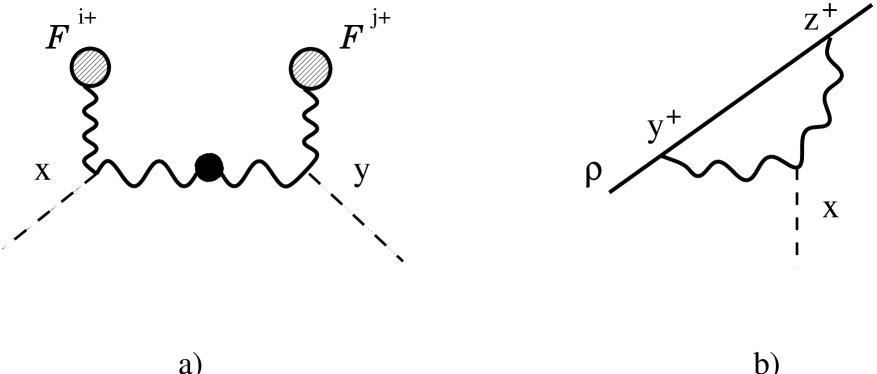
To gain some more intuition, we use as an example the contributions to $\delta\hat{\rho}_{a}$ coming from the Yang-Mills piece of the action, $S_{YM}=\int d^{4}x(-F_{\mu\nu}^{2}/4)$ :

$$\delta\hat{\rho}_{a}(x)\big{|}_{YM}\,=\,2gf^{abc}{\cal F}^{+i}_{b}(\vec{x})a^{i}_{c}(x)+gf^{abc}(\partial^{+}a_{b}^{i}(x))a_{c}^{i}(x).$$ (3.38)

The first term in the r.h.s., which is linear in $a^{i}$, is the only one to contribute to $\chi$, eq. (3.30), to leading order in $\alpha_{s}$. It generates the tree-like diagram in Fig. 17.a, where the internal line with a blob represents the background field propagator $G^{ij}(x,y)$ of the semi-fast gluons. Physically, Fig. 17.a describes the emission of an on-shell (or “real”) semi-fast gluon by the classical source.

Since $\langle a^{i}\rangle=0$, it is only the second, quadratic term in the r.h.s. of eq. (3.38) which contributes to $\sigma$, eq. (3.29). In Fig. 17.b we show such a contribution of lowest order in $\rho\,$. (This involves also vertices from the Wilson line piece of the action, eqs. (3.10)–(3.11).) Obviously, this represents a vertex correction to the tree-level emission in Fig. 10.a.

The structures illustrated by Figs. 17.a and b are generic: $\chi$ is the “real” correction, whose iteration generates the gluon cascades; $\sigma$ is the “virtual” correction, which provides one-loop corrections to the emission vertices in these cascades. Both $\chi$ and $\sigma$ include terms non-linear in $\rho$ which describe interactions among gluons at different rapidities in different cascades. In general, real and virtual corrections are related by gauge symmetry, and this is also the case for $\chi$ and $\sigma$, as we shall discuss later.

The diagrams contributing to $\sigma$ and $\chi$ in the general case, together with their explicit evaluation, can be found in Ref. [37]. Here, we shall present only the final results of this calculation.

3.4.2 The induced colour source and field

For the reasons explained in Sect. 2.3, it is more convenient to work with the colour source $\tilde{\rho}_{a}$ in the covariant gauge. The corresponding weight function $W_{\tau}[\tilde{\rho}]$ obeys an evolution equation similar to (3.31), but with modified coefficients $\tilde{\sigma}$ and $\tilde{\chi}$, which are obtained from the LC-gauge coefficients $\sigma$ and $\chi$ via the gauge rotation (2.36). In what follows, we shall give directly the final results for these COV-gauge quantities.

Consider first the induced source $\delta\rho^{a}=\langle\delta\hat{\rho}^{a}\rangle_{\rho}$, that is, the correction to the average colour charge density generated by the polarization of the semi-fast gluons. After rotation to the COV-gauge, this reads [37] :

$$\delta\tilde{\rho}_{a}(\vec{x})\,=\,F_{\Lambda}(x^{-})(-\nabla_{\perp}^{2}\nu_{a}(x_{\perp})),$$ (3.39)

where the “form factor”

$$F_{\Lambda}(x^{-})\,\equiv\,\theta(x^{-})\,\frac{e^{-ib\Lambda x^{-}}-e^{-i\Lambda x^{-}}}{x^{-}}\,,$$ (3.40)

specifies the longitudinal profile of $\delta\tilde{\rho}_{a}$, while ($V^{\dagger}_{x}\equiv V^{\dagger}(x_{\perp})$, cf. eq. (2.45))

$$\nu^{a}(x_{\perp}) = {ig\over 2\pi}\int{d^{2}z_{\perp}\over(2\pi)^{2}}\,\frac{1}{(x_{\perp}-z_{\perp})^{2}}\,{\rm Tr}\Bigl{(}T^{a}V^{\dagger}_{x}V_{z}\Bigr{)}$$ (3.41)

contains the dependence upon the background field $\alpha_{a}$ (via the Wilson lines $V$ and $V^{\dagger}$), together with the transverse and colour structure of $\delta\tilde{\rho}_{a}$. By comparing eqs. (3.39) and (2.33), we deduce that $F(x^{-})\nu^{a}(x_{\perp})$ is the induced field in the COV-gauge, i.e., the quantum correction to the tree-level field $\alpha_{a}$. Since:

$$\int dx^{-}F_{\Lambda}(x^{-})\,=\,\ln{1\over b}\,=\,\Delta\tau,$$ (3.42)

eqs. (3.29) and (3.39) immediately imply :

$$\tilde{\sigma}_{a}(x_{\perp}) = -\nabla_{\perp}^{2}\nu_{a}(x_{\perp}).$$ (3.43)

This is the coefficient of the virtual term in the RGE for $W_{\tau}[\tilde{\rho}]$.

But the longitudinal structure of $\delta\tilde{\rho}_{a}$ is also interesting. Eq. (3.39) shows that the induced source and field have typically support at

$$1/\Lambda^{+}\,\,\mathrel{\hbox to0.0pt{\raise 2.20013pt\hbox{$<$}\hss}{\lower 2.20013pt\hbox{$\sim$}}}\,\,x^{-}\,\,\mathrel{\hbox to0.0pt{\raise 2.20013pt\hbox{$<$}\hss}{\lower 2.20013pt\hbox{$\sim$}}}\,\,1/(b\Lambda^{+})\,.$$ (3.44)

Recall that $\delta\tilde{\rho}_{a}$ has been generated by integrating out quantum fluctuations in the strip $b\Lambda^{+}\ll|p^{+}|\ll\Lambda^{+}$. Thus, when integrating out quantum gluons in layers of $p^{+}$, one builds the classical source $\rho$ (or field $\alpha$) in layers of $x^{-}$, with a one-to-one correspondence between the $x^{-}$ coordinate of a given layer and the $p^{+}$ momenta of the modes that have been integrated out to generate that layer. By induction, we deduce that $\rho_{a}(\vec{x})$ ($\equiv$ the colour source generated by the quantum evolution down to $\Lambda^{+}$) has support at $0\leq x^{-}\mathrel{\hbox to0.0pt{\raise 2.20013pt\hbox{$<$}\hss}{\lower 2.20013pt\hbox{$\sim$}}}1/\Lambda^{+}$, as anticipated in Sect. 2. This allows us to consider only positive values for $x^{-}$ in what follows.

To exploit this tight correspondence between $p^{+}$ and $x^{-}$, it is convenient to use the space-time rapidity y,

$${\rm y}\,\equiv\,\ln(x^{-}/x^{-}_{0}),\quad x^{-}_{0}\equiv 1/P^{+}\,,\quad-\infty<{\rm y}<\infty\,,$$ (3.45)

to indicate the longitudinal coordinate of a field. We shall set, e.g.,

$$\rho_{{\rm y}}^{a}(x_{\perp}) \equiv x^{-}\rho^{a}(x^{-},x_{\perp})\qquad{\rm for}\quad x^{-}=x^{-}_{\rm y}\equiv x^{-}_{0}{\rm e}^{{\rm y}},$$

$$\int d{\rm y}\,\rho_{{\rm y}}^{a}(x_{\perp}) = \int dx^{-}\,\rho^{a}(x^{-},x_{\perp}),$$ (3.46)

and similarly for the other fields ($\tilde{\rho}$, $\alpha$, etc.). The previous discussion on the longitudinal structure can then be summarized as follows:

The source $\rho_{{\rm y}}^{a}(x_{\perp})$ generated by the quantum evolution from $\tau^{\prime}=0$ up to $\tau$ has support at y in the interval $0\leq{\rm y}\leq\tau$. When new quantum modes, with rapidities $\tau^{\prime}$ in the interval $\tau<\tau^{\prime}<\tau+\Delta\tau$, are integrated out, the preexisting colour source at ${\rm y}\leq\tau$ is not changed, but some new contribution is added to it, in the rapidity bin $\tau<{\rm y}<\tau+\Delta\tau$. Because of that, $\Delta W\equiv W_{\tau+\Delta\tau}-W_{\tau}$ involves only the change in $\rho_{\rm y}$ within that last bin. In the continuum limit $\Delta\tau\to 0$, this generates the functional derivatives of $W_{\tau}$ with respect to $\rho_{\rm y}^{a}$ at ${\rm y}=\tau$, as shown in eq. (3.31). This clarifies the longitudinal structure of the RGE.

Consider also the transverse and colour structure of the induced field (3.41). This can be understood by reference to Fig. 17.b. The transverse kernel in eq. (3.41) has been generated as:

$${1\over(2\pi)^{2}}\,\frac{1}{(x_{\perp}-z_{\perp})^{2}}\,=\,{1\over 2\pi}\frac{x^{i}-z^{i}}{(x_{\perp}-z_{\perp})^{2}}\,{1\over 2\pi}\frac{x^{i}-z^{i}}{(x_{\perp}-z_{\perp})^{2}}\,,$$ (3.47)

where (compare with eqs. (2.34) and (2.53))

$${1\over 2\pi}\frac{x^{i}-z^{i}}{(x_{\perp}-z_{\perp})^{2}}=\partial^{i}_{x}\langle x_{\perp}|\,\frac{1}{-\nabla^{2}_{\perp}}\,|z_{\perp}\rangle\,=\int{d^{2}p_{\perp}\over(2\pi)^{2}}\,{-i\,p^{i}\over p_{\perp}^{2}}\,{\rm e}^{ip_{\perp}\cdot(x_{\perp}-z_{\perp})}$$ (3.48)

is the propagator of the semi-fast gluon emitted by the source $\rho$ (recall that ${\cal F}^{+j}\approx(ip^{j}/p_{\perp}^{2})\rho$ to linear order). The two Wilson lines in eq. (3.41) account for the scattering of this semi-fast gluon off the background field at $z_{\perp}$ (this brings in a factor $V^{\dagger}(z_{\perp})$ in the eikonal approximation), and for its gauge rotation by the classical field ${\cal A}^{i}(\vec{x})$ at $x^{-}>1/\Lambda^{+}$ (cf. eq. (3.44)), which is a pure gauge (cf. eq. (2.43)).

3.4.3 The RGE in the $\alpha$–representation

Eq. (3.43) suggests that it may be technically simpler and physically more transparent to work directly with the classical field $\alpha_{a}$ and the quantum corrections to it (like $\nu_{a}$), rather than with the colour source $\tilde{\rho}_{a}$ and the corresponding corrections (like $\tilde{\sigma}_{a}$). This point of view is also supported by the fact that the LC-gauge field and the related observables are primarily related to $\alpha_{a}$ (cf. Sects. 2.2 and 2.3), and reexpressing them in terms of $\tilde{\rho}$ — with the help of eq. (2.34) — would introduce a dependence upon the unphysical infrared cutoff $\mu$.

For these reasons, we prefer to work in the $\alpha$–representation, in which observables are expressed in terms of $\alpha$, and the average is performed with the weight function $W_{\tau}[\alpha]\equiv W_{\tau}[\tilde{\rho}=-\nabla_{\perp}^{2}\alpha]$. This satisfies the following RGE, which is obtained after a change of variables in eq. (3.31) :

$${\partial W_{\tau}[\alpha]\over{\partial\tau}}\,=\,{1\over 2}{\delta^{2}\over{\delta\alpha_{\tau}^{a}(x_{\perp})\delta\alpha_{\tau}^{b}(y_{\perp})}}\,[W_{\tau}\eta_{xy}^{ab}]-{\delta\over{\delta\alpha_{\tau}^{a}(x_{\perp})}}\,[W_{\tau}\nu_{x}^{a}]\,,$$ (3.49)

where $\nu_{x}^{a}\equiv\nu^{a}(x_{\perp})$, cf. eq. (3.41), and $\eta_{xy}^{ab}\equiv\eta^{ab}(x_{\perp},y_{\perp})$, with

$$\eta^{ab}(x_{\perp},y_{\perp})\equiv\int d^{2}z_{\perp}d^{2}u_{\perp}\langle x_{\perp}|\frac{1}{-\nabla^{2}_{\perp}}|z_{\perp}\rangle\,\tilde{\chi}^{ab}(z_{\perp},u_{\perp})\,\langle u_{\perp}|\frac{1}{-\nabla^{2}_{\perp}}|y_{\perp}\rangle.\,\,\,\,\,\,$$ (3.50)

It is thus sufficient to give the result for the “real correction” $\langle\delta\hat{\rho}_{a}\delta\hat{\rho}_{b}\rangle_{\rho}$ directly in the $\alpha$-representation (cf. eqs. (3.30) and (3.50)). This reads [37]:

$$\eta^{ab}(x_{\perp},y_{\perp}) = {1\over\pi}\!\int{d^{2}z_{\perp}\over(2\pi)^{2}}\,\frac{(x^{i}-z^{i})(y^{i}-z^{i})}{(x_{\perp}-z_{\perp})^{2}(y_{\perp}-z_{\perp})^{2}}$$ (3.51)

$$\qquad\quad\times\,\,\Bigl{\{}1+V^{\dagger}_{x}V_{y}-V^{\dagger}_{x}V_{z}-V^{\dagger}_{z}V_{y}\Bigr{\}}^{ab}.$$

The transverse and colour structure of $\eta$ have the same pattern as discussed after eq. (3.53) in connection with $\nu$.

The r.h.s. of eq. (3.49) involves functional derivatives w.r.t. the colour field $\alpha_{\tau}^{a}(x_{\perp})$ at the end point ${\rm y}=\tau$. When applied to the coefficients $\eta$ and $\nu$, this requires the corresponding derivatives of the Wilson lines $V$ and $V^{\dagger}$, that we compute now. Note first that, since $\alpha_{{\rm y}}=0$ for ${\rm y}>\tau$, we can rewrite

$$V^{\dagger}(x_{\perp})\,\equiv\,{\rm P}\,{\rm e}^{ig\int_{-\infty}^{\infty}d{\rm y}\,\alpha_{{\rm y}}(x_{\perp})}\,=\,{\rm P}{\,\rm e}^{ig\int_{-\infty}^{\tau}d{\rm y}\,\alpha_{{\rm y}}(x_{\perp})}.$$ (3.52)

Therefore (with $\delta_{xy}\equiv\delta^{(2)}(x_{\perp}-y_{\perp})$):

$${\delta V^{\dagger}(x_{\perp})\over\delta\alpha^{a}_{\tau}(y_{\perp})}=ig\delta_{xy}T^{a}V^{\dagger}(x_{\perp}),\quad{\delta V(x_{\perp})\over\delta\alpha^{a}_{\tau}(y_{\perp})}=-ig\delta_{xy}V(x_{\perp})T^{a}\,.$$ (3.53)

A simple interpretation of the four terms in eq. (3.51) follows from the dual picture of the dipole-hadron scattering, in which the quantum evolution is put in the dipole wavefunction, and, more generally, in the Wilson line operators through which a generic external projectile scatters off the hadronic target [44, 45, 46, 47, 48, 49, 50, 51]. (See also the lectures notes by Al Mueller in this volume [14].) Recent analyses of the high energy scattering from this dual perspective have led to a set of coupled evolution equations for the correlation functions of Wilson lines, originally derived by Balitsky [44] (see also [45, 50]), and subsequently reformulated by Weigert [47] in a compact way, as a functional evolution equation for the generating functional of these correlation functions. It turns out that Weigert’s equation is equivalent to the RGE (3.49) [37, 52], which demonstrates the equivalence between the two descriptions — the target picture and the projectile picture — of the nonlinear evolution in QCD at small x. We shall say more on Balitsky’s equations in Sect. 4.3.

3.5 Recovering the BFKL equation

Before studying more general properties and consequences of the RGE in the next section, let us rapidly show that, in the weak field (or low density) limit, this equation reproduces the BFKL equation, as expected [36]. Eq. (3.32) implies the following evolution equation for the 2-point function $\langle\rho\rho\rangle_{\tau}\,$:

$${d\over{d\tau}}\langle\rho_{a}(x_{\perp})\rho_{b}(y_{\perp})\rangle_{\tau}\!=\!\langle\sigma_{a}(x_{\perp})\rho_{b}(y_{\perp})+\rho_{a}(x_{\perp})\sigma_{b}(y_{\perp})+\chi_{ab}(x_{\perp},y_{\perp})\rangle_{\tau}\,\,\,\,\,\,\,\,$$ (3.54)

For a generic, strong, source $\rho$, the coefficients $\sigma$ and $\chi$ are non-linear in $\rho$ to all orders, so the r.h.s. of eq. (3.54) involves $n$-point correlators $\langle\rho(1)\rho(2)\cdots\rho(n)\rangle_{\tau}$ of arbitrarily high order $n$. But in the weak field limit, where $\sigma$ is linear in $\rho$ and $\chi$ is quadratic, this becomes a closed equation for the 2-point function, which coincides with the BFKL equation, as we show now.

Specifically, consider the evolution equation for the following 2-point function:

$$\mu_{\tau}(k^{2}_{\perp})\,\equiv\,\langle\rho_{a}(k_{\perp})\rho_{a}(-k_{\perp})\rangle_{\tau},$$ (3.55)

($\rho_{a}(k_{\perp})$ is the Fourier transform of $\rho_{a}(x_{\perp})$), which according to eqs. (2.16) and (2.54) represents the “unintegrated gluon distribution” :

$${\partial\,{\rm x}G({\rm x},k^{2}_{\perp})\over\partial\ln k^{2}_{\perp}}\,\propto\,\mu_{\tau}(k^{2}_{\perp}),$$ (3.56)

in the weak field regime. In this regime, one can also expand $V^{\dagger}_{x}\approx 1+ig\alpha(x_{\perp})$, and therefore

$${\rm Tr}\bigl{(}T^{a}V^{\dagger}_{x}V_{z}\bigr{)}\approx igN_{c}(\alpha^{a}(x_{\perp})-\alpha^{a}(z_{\perp})).$$

Then, eq. (3.41) reduces to (with $\alpha_{s}=g^{2}/4\pi$ and $k^{2}_{\perp}\alpha_{a}(k_{\perp})=\rho_{a}(k_{\perp})$) :

$$\sigma^{(0)}_{a}(k_{\perp})\,=\,-\alpha_{s}N_{c}\,\rho_{a}(k_{\perp})\int\frac{d^{2}p_{\perp}}{(2\pi)^{2}}\,{k^{2}_{\perp}\over p_{\perp}^{2}(p_{\perp}-k_{\perp})^{2}}\,.$$ (3.57)

For $\chi$ one obtains similarly

$$\chi^{(0)}_{aa}(k_{\perp},-k_{\perp})\,=\,4\alpha_{s}N_{c}k_{\perp}^{2}\int\frac{d^{2}p_{\perp}}{(2\pi)^{2}}\,\frac{\rho_{a}(p_{\perp})\rho_{a}(-p_{\perp})}{p^{2}_{\perp}(k_{\perp}-p_{\perp})^{2}}\,.$$ (3.58)

By inserting eqs. (3.57) and (3.58) into the evolution equation (3.54), and using (3.55), one finally obtains:

$${\partial\mu_{\tau}(k^{2}_{\perp})\over\partial\tau} = \,\,\,{\alpha_{s}N_{c}\over\pi^{2}}\,\int d^{2}p_{\perp}{k^{2}_{\perp}\over p^{2}_{\perp}(k_{\perp}-p_{\perp})^{2}}\,\mu_{\tau}(p^{2}_{\perp})$$ (3.59)

$$-\,{\alpha_{s}N_{c}\over 2\pi^{2}}\,\int d^{2}p_{\perp}{k^{2}_{\perp}\over p^{2}_{\perp}(k_{\perp}-p_{\perp})^{2}}\,\mu_{\tau}(k^{2}_{\perp})\,,$$

which coincides, as anticipated, with the BFKL equation [3, 4]. The first term in the r.h.s., which here is generated by $\chi^{(0)}$, is the real BFKL kernel, while the second term, coming from $\sigma^{(0)}$, is the corresponding virtual kernel.

Note finally that the BFKL approximation has been obtained by expanding the Wilson lines to linear order in $g\alpha^{a}$; thus, this is formally the same as the lowest order perturbative expansion of the RGE.

4 A functional Fokker-Planck equation

We now dispose of a powerful tool — the functional RGE (3.49) — to construct the effective theory by integrating out quantum fluctuations in perturbation theory. Eq. (3.49) has a rich and elegant mathematical structure, to be described in Sects. 4.1 and 4.2. Then, in Sects. 4.3 and 5, we shall indicate two strategies to make use of this equation:

i) One can use it to derive ordinary (i.e., non-functional) evolution equations for the correlation functions of interest, like we did for the 2-point function $\langle\rho\rho\rangle_{\tau}\,$ in Sect. 3.5. When specialized to correlation functions of the Wilson lines, this strategy leads to a system of equations originally derived by Balitsky [44]. This will be discussed in Sect. 4.3.

A difficulty with this approach is that it generally leads to coupled equations (the 2-point function is coupled to the 4-point one, etc.), so that one has to follow simultaneously the evolution of infinitely many correlators. Still, some progress has been done, by using functional techniques [53], and, especially, by recognizing that, in the large $N_{c}$ limit, a closed equation can be written for the 2-point function: this is the Kovchegov equation [45].

ii) One can try and solve directly the functional RGE, with appropriate initial conditions. An exact but formal solution can be written in the form of a path integral [52]. This is well suited for lattice simulations in 2+1 dimensions. But approximate analytic solutions, which allow for a more direct physical insight, have been found as well [10, 57]. These solutions will be described in Sect. 5.

4.1 General properties and consequences of the RGE

We start with a summary of the most important properties of the RGE (3.49).

i) The coefficients $\eta$ and $\nu$ are real quantities. Moreover, $\eta$ is symmetric: $\eta_{ab}(x_{\perp},y_{\perp})=\eta_{ba}(y_{\perp},x_{\perp})$, and positive semi-definite.

ii) The RGE preserves the normalization of the weight function:

$$\int{\cal D}\alpha\,\,W_{\tau}[\alpha]\,=\,1\qquad{\rm at\,\,any}\,\,\tau.$$ (4.1)

Indeed, the r.h.s. of eq. (3.49) is a total derivative with respect to $\alpha$. Thus, if eq. (4.1) is satisfied by the initial condition at $\tau_{0}$, it remains true at any $\tau>\tau_{0}$.

Properties (i) and (ii) guarantee that the solution $W_{\tau}[\alpha]$ to the RGE has a meaningful probabilistic interpretation (cf. the discussion prior to eq. (2.4)).

iii) The momentum rapidity $\tau$ and the space-time rapidity ${\rm y}$ are identified by the quantum evolution. That is, the field $\alpha_{\rm y}$ in the rapidity bin $({\rm y},\,{\rm y}+d{\rm y})$ is generated by the quantum evolution from $\tau={\rm y}$ up to $\tau={\rm y}+d{\rm y}$. This follows from the discussion in Sect. 3.4.2, and implies that the two rapidities can be treated as only one variable, the “evolution time”.

With this interpretation, the function $\{\alpha_{{\rm y}}^{a}(x_{\perp})\,|\,-\infty<{\rm y}<\infty\}$ — which physically represents the longitudinal profile of the 3-dimensional field $\alpha^{a}(x^{-},x_{\perp})$ in units of rapidity (cf. eq. (3.4.2)) — is viewed as a trajectory in the functional space spanned by the 2-dimensional fields $\alpha^{a}(x_{\perp})$. Quantum evolution then appears as the progression of the “point” $\alpha^{a}(x_{\perp})$ along this trajectory. Thus, eq. (3.49) describes effectively a field theory in 2+1 dimensions (the transverse coordinates and the “evolution time”), which is however non-local in both $x_{\perp}$ and ${\rm y}$ (since the coefficients (3.41) and (3.51) of the RGE involve $\alpha_{\rm y}$ at all the “times” ${\rm y}\leq\tau$, via the Wilson lines (3.52)).

iv) The initial condition. Let the quantum evolution proceed from some original “time” $\tau_{0}$ up to the actual “time” $\tau$. The “trajectory” $\{\alpha_{{\rm y}}^{a}(x_{\perp})\,|\,-\infty<{\rm y}<\infty\}$ can be decomposed into three pieces: a) The field $\alpha_{\rm y}$ at ${\rm y}\leq\tau_{0}$ belongs to the initial conditions. b) The field $\alpha_{\rm y}$ at $\tau_{0}<{\rm y}\leq\tau$ is generated by the quantum evolution. c) There is no field at all at larger ${\rm y}$: $\alpha_{{\rm y}}=0$ for any ${\rm y}>\tau$. Thus:

$$W_{\tau}[\alpha]\,=\,\delta[\alpha^{>}]\,{\cal W}_{\tau}[\alpha^{<}],$$ (4.2)

where $\alpha^{<}_{{\rm y}}$ ($\alpha^{>}_{{\rm y}}$) is the function $\alpha_{{\rm y}}$ for ${\rm y}<\tau$ (respectively, ${\rm y}>\tau$) :

$$\alpha_{{\rm y}}(x_{\perp})\,\equiv\,\theta(\tau-{\rm y})\alpha^{<}_{{\rm y}}(x_{\perp})\,+\,\theta({\rm y}-\tau)\alpha^{>}_{{\rm y}}(x_{\perp}),$$ (4.3)

and the $\delta$–functional $\delta[\alpha^{>}]$ should be understood with a discretization of the configuration space, as in eq. (2.5):

$$\delta[\alpha^{>}]\,\equiv\,\prod_{{\rm y}>\tau}\prod_{a}\prod_{x_{\perp}}\,\delta(\alpha_{{\rm y}}^{a}(x_{\perp})).$$ (4.4)

Moreover, it can be shown [10, 52] that ${\cal W}_{\tau}[\alpha^{<}]$ has the factorized structure:

$${\cal W}_{\tau}[\alpha^{<}]\,=\,{\cal W}_{\tau,\,\tau_{0}}[\alpha|V_{0}]\,{\cal W}_{\tau_{0}}[\alpha]\,,$$ (4.5)

where ${\cal W}_{\tau_{0}}[\alpha]$ is the initial weight function at $\tau_{0}\,$, and

$$V_{0}^{\dagger}(x_{\perp})\,\equiv\,{\rm P}\,{\rm e}^{ig\int_{-\infty}^{\tau_{0}}d{\rm y}\,\alpha_{{\rm y}}(x_{\perp})}$$ (4.6)

is the Wilson line built with the initial field. In eq. (4.5), it is understood that, in ${\cal W}_{\tau_{0}}$, the field argument $\alpha_{\rm y}$ has support at ${\rm y}\leq\tau_{0}$, while in ${\cal W}_{\tau,\,\tau_{0}}$ it has support at $\tau_{0}<{\rm y}\leq\tau$. The “propagator” ${\cal W}_{\tau,\,\tau_{0}}$ from $\tau_{0}$ to $\tau$ depends also upon the initial field at ${\rm y}\leq\tau_{0}$, but only in an integrated way, via the Wilson lines $V_{0}$ and $V_{0}^{\dagger}$. From eq. (4.5) we deduce that ${\cal W}_{\tau,\,\tau_{0}}[\alpha|V_{0}]\to 1$ when $\tau\to\tau_{0}$.

The initial weight function ${\cal W}_{\tau_{0}}$ cannot be obtained within the present formalism, but rather requires some model for the hadron wavefunction at rapidity $\tau_{0}$. It is convenient to choose a moderate value for $\tau_{0}=\ln(1/{\rm x}_{0})$, e.g., ${\rm x}_{0}\simeq 10^{-2}$. This ${\rm x}_{0}$ is small enough for the LLA to apply, but still large enough for the non-linear effects to remain negligible. Then one can use initial conditions which are consistent with the standard, linear, evolution equations (cf. Sect. 5.3 below). Once a convenient value for ${\rm x}_{0}$ has been chosen, one can always redefine $\tau\equiv\ln({\rm x}_{0}/{\rm x})$ so that the initial condition is formulated at $\tau_{0}=0$. With this choice, the field $\alpha_{{\rm y}}$ at positive rapidities ${\rm y}>0$ is generated by the quantum evolution, while the field at negative rapidities ${\rm y}<0$ must be specified by the initial condition.

v) The Hamiltonian structure of the RGE. Eq. (3.49) can be rewritten as:

$${\partial W_{\tau}[\alpha]\over{\partial\tau}}\,=\,{\delta\over{\delta\alpha_{\tau}^{a}(x_{\perp})}}\left\{{1\over 2}\eta_{xy}^{ab}\,{\delta W_{\tau}\over{\delta\alpha_{\tau}^{b}(y_{\perp})}}+\left({1\over 2}\,{\delta\eta_{xy}^{ab}\over{\delta\alpha_{\tau}^{b}(y_{\perp})}}-\nu_{x}^{a}\right)W_{\tau}\right\}\,,$$ (4.7)

A crucial property, with many consequences, is that the second term within the braces is actually zero. Indeed, the following relation holds between the coefficients of the RGE [47, 37]:

$${1\over 2}\int d^{2}y_{\perp}{\delta\eta^{ab}(x_{\perp},y_{\perp})\over{\delta\alpha_{\tau}^{b}(y_{\perp})}}\,=\,\nu^{a}(x_{\perp})\,.$$ (4.8)

It is easy to prove this relation by using eq. (3.53) to act with $\delta/\delta\alpha_{\tau}^{b}(y_{\perp})$ on $\eta_{ab}(x_{\perp},y_{\perp})$, eq. (3.51). This yields, e.g.,

$${\delta\over{\delta\alpha_{\tau}^{b}(y_{\perp})}}\,(V^{\dagger}_{x}V_{y})^{ab} = {\delta V^{\dagger\,ac}_{x}\over{\delta\alpha_{\tau}^{b}(y_{\perp})}}\,V_{y}^{cb}\,+\,V^{\dagger\,ac}_{x}{\delta V_{y}^{cb}\over{\delta\alpha_{\tau}^{b}(y_{\perp})}}$$

$$= ig\delta_{xy}\Bigl{(}T^{b}V^{\dagger}_{y}\Bigr{)}_{ac}V_{y}^{cb}-ig\delta^{(2)}(0_{\perp})V^{\dagger\,ac}_{x}\Bigl{(}V_{y}T^{b}\Bigr{)}_{cb}\,=\,0,$$

where both terms in the second line vanish because of the antisymmetry of the colour group generators in the adjoint representation (e.g., $(T^{b})_{ab}=0$). The only nonvanishing contribution is

$$-{\delta\over{\delta\alpha_{\tau}^{b}(y_{\perp})}}\,(V^{\dagger}_{x}V_{z})^{ab}\,=\,-ig\delta_{xy}\Bigl{(}T^{b}V^{\dagger}_{x}V_{z}\Bigr{)}_{ab}\,=\,ig\delta_{xy}{\rm Tr}\Bigl{(}T^{a}V^{\dagger}_{x}V_{z}\Bigr{)},$$ (4.10)

which reproduces indeed eq. (3.41) after integration over $y_{\perp}$, since:

$${\cal K}(x_{\perp},y_{\perp},z_{\perp})\equiv\frac{(x^{i}\!-\!z^{i})(y^{i}\!-\!z^{i})}{(x_{\perp}\!-\!z_{\perp})^{2}(y_{\perp}\!-\!z_{\perp})^{2}}\rightarrow\frac{1}{(x_{\perp}\!-\!z_{\perp})^{2}}\,\,\,\,{\rm for}\,\,\,\,y_{\perp}\!\to\!x_{\perp}.\,\,\,\,$$ (4.11)

With eqs. (4.7) and (4.8), the RGE can be brought into a Hamiltonian form:

$${\partial W_{\tau}[\alpha]\over{\partial\tau}}\,=\,-\,HW_{\tau}[\alpha],$$ (4.12)

with the following Hamiltonian:

$$H \equiv {1\over 2}\int\!d^{2}x_{\perp}\!\int d^{2}y_{\perp}{i\delta\over{\delta\alpha_{\tau}^{a}(x_{\perp})}}\,\eta_{xy}^{ab}\,{i\delta\over{\delta\alpha_{\tau}^{b}(y_{\perp})}}\,=\!\int\!{d^{2}z_{\perp}\over 2\pi}\,J^{i}_{a}(z_{\perp})J^{i}_{a}(z_{\perp}),$$

$$J^{i}_{a}(z_{\perp}) \equiv \int{d^{2}x_{\perp}\over 2\pi}\,\frac{z^{i}-x^{i}}{(z_{\perp}-x_{\perp})^{2}}\,(1-V^{\dagger}_{z}V_{x})_{ab}\,{i\delta\over{\delta\alpha_{\tau}^{b}(x_{\perp})}}\,,$$ (4.13)

which is Hermitian (since $\eta_{xy}^{ab}$ is real and symmetric) and positive semi-definite (since the “current” $J^{i}_{a}(z_{\perp})$ is itself Hermitian).

vi) The infrared and ultraviolet behaviours of the RGE. These are determined by the kernel $\eta^{ab}(x_{\perp},y_{\perp})$ in the Hamiltonian. In the infrared limit, where $z_{\perp}$ is much larger than both $x_{\perp}$ and $y_{\perp}$ (see eq. (3.51)), ${\cal K}(x_{\perp},y_{\perp},z_{\perp})\approx 1/z_{\perp}^{2}$, and the ensuing integral $(d^{2}z_{\perp}/z_{\perp}^{2})$ has a logarithmic infrared divergence. Thus, there is potentially an IR problem in the RGE. This is not necessarily a real difficulty, since IR problems are expected to be absent only for the gauge-invariant observables. We shall see indeed, on specific examples, that the IR divergences cancel when the RGE is used to derive evolution equations for gauge-invariant quantities. This cancellation relies in a crucial way on the property (4.8).

Coming now to the ultraviolet, or short-distance, behaviour, it is easy to see on eq. (3.51) that no UV problem is to be anticipated. For instance, the would-be linear pole of ${\cal K}(x_{\perp},y_{\perp},z_{\perp})$ at $|z_{\perp}-x_{\perp}|\to 0$ is actually cancelled by the factor $1-V^{\dagger}_{z}V_{x}$ which vanishes in the same limit.

4.2 Quantum evolution as Brownian motion

To clarify the probabilistic interpretation of the RGE (3.49), we start by recalling the simplest example of a stochastic process, namely the Brownian motion of a small particle in a viscous liquid and in the presence of some external force, like gravitation [59]. The particle is so small that it can feel the collisions with the molecules in the liquid; after each such a collision, the velocity of the particle changes randomly. And the liquid is so viscous that, after each collision, the particle enters immediately a constant velocity regime in which the friction force $\propto v^{i}$ (with $v^{i}$ the velocity of the particle) is equilibrated by the random force due to collisions together with the external force $F^{i}(x)$. In these conditions, the particle executes a random walk whose description is necessary statistical. The relevant quantity is the probability density $P(x,t)$ to find the particle at point $x$ at time $t$. This is normalized as:

$$\int d^{3}x\,P(x,t)\,=\,1,$$ (4.14)

and obeys an evolution equation of the diffusion type, known as the Fokker-Planck equation [59] :

$${\partial P(x,t)\over{\partial t}}\,=\,D{\partial^{2}\over\partial x^{i}\partial x^{i}}\,P(x,t)\,-\,{\partial\over\partial x^{i}}\Bigl{(}F^{i}(x)P(x,t)\Bigr{)}.$$ (4.15)

Here, $D$ is the diffusion coefficient, which is a measure of the strength of the random force; for simplicity, we assume this to be a constant, i.e., independent of $x$ or $t$. The solution to eq. (4.15) corresponding to some arbitrary initial condition $P(x,t_{0})$ can be written as

$$P(x,t)\,=\,\int d^{3}x_{0}\,P(x,t|x_{0},t_{0})\,P(x_{0},t_{0}),$$ (4.16)

where $P(x,t|x_{0},t_{0})$ is the solution to (4.15) with the initial condition:

$$P(x,t_{0}|x_{0},t_{0})\,=\,\delta^{(3)}(x-x_{0}).$$ (4.17)

Physically, this is the probability density to find the particle at point $x$ at time $t$ knowing that it was at $x_{0}$ at time $t_{0}$.

If $F^{i}=0$, this solution is immediately obtained by going to momentum space: The Fourier transform $\tilde{P}(k,t)$ of $P(x,t_{0}|x_{0},0)\equiv P(x-x_{0},t)$ obeys to:

$${\partial\tilde{P}(k,t)\over{\partial t}}\,=\,-Dk^{2}\,\tilde{P}(k,t),\qquad\tilde{P}(k,t=0)\,=\,1,$$ (4.18)

with the obvious solution $\tilde{P}(k,t)={\rm e}^{-Dk^{2}t}$, or, finally,

$$P(x-x_{0},t)\,=\,{1\over(4\pi Dt)^{3/2}}\,\,{\rm e}^{-\frac{({x-x_{0}})^{2}}{4Dt}}.$$ (4.19)

This shows a purely diffusive behaviour: the probability to find the particle within a fixed volume centered at some point $x$ goes smoothly to zero as $t\to\infty$ for any $x$ (runaway solution). The correlations of $x$ reflect this behaviour too; for instance:

$$\overline{r^{2}}(t)\,\equiv\,\langle({x-x_{0}})^{2}\rangle(t)\,\equiv\int d^{3}x\,({x-x_{0}})^{2}\,P(x-x_{0},t)\,=\,6Dt,$$ (4.20)

showing that, on the average, the particle gets further and further away from the original point $x_{0}$, but along a non-differentiable trajectory: $\bar{r}(t)\propto\sqrt{t}$, so the average velocity $\bar{v}=\bar{r}(\Delta t)/\Delta t$ has no well-defined limit when $\Delta t\to 0$.

This situation may change, however, if the motion of the particle is biased by an external force. Assume this force to be derived from a potential: $F^{i}=-{\partial V/\partial x^{i}}$. Then one can check that the time-independent distribution $P_{0}(x)\sim{\rm exp}[-\beta V(x)]$ is a stationary solution to eq. (4.15) provided $\beta D=1$. Of course, this solution is acceptable as a probability density only if it is normalizable, which puts some constraints on the form of the potential. But assuming this to be the case, then $P_{0}(x)\sim{\rm e}^{-\beta V}$ represents an equilibrium distribution which is (asymptotically) reached by the system at large times [59]. Once this is done, all the correlations become independent of time (unlike (4.20)). This solution is a “fixed point” in the functional space of all (acceptable) distributions.

Returning to our RGE (3.49), it should be clear by now that this is a functional Fokker-Planck equation which describes a random walk in the functional space of the colour fields $\alpha^{a}(x_{\perp})$. In this equation, $\eta$ plays the role of the “diffusion coefficient”, while $\nu$ is like a “force term”, although this identification is somehow ambiguous since $\eta$ is itself a functional of $\alpha$, so its derivatives can generate other contributions to the force term, as shown in eq. (4.7). (In the analogous problem of the Brownian motion, this would correspond to a diffusion coefficient which depends on $x$ and has a tensorial structure: $D\to D_{ij}(x)$. This situation occurs, e.g., in the description of a random walk on a curved manifold [59].) In fact, it is more correct to identify the combination ${1\over 2}({\delta\eta/{\delta\alpha_{\tau}}})-\nu\,$ as the effective “force term”, since the remaining second-order differential operator in eq. (4.7) — which describes diffusion — is then Hermitian and positive semi-definite.

A fixed point of the quantum evolution would be a solution $W[\alpha]$ to eq. (3.49) which is normalizable and independent of “time” $\tau$. If such a solution existed, then the high energy limit of QCD scattering would be trivial (at least, within the present approximations): At sufficiently high energies, all the cross sections would become independent of energy (recall that $\tau\sim\ln s$). The relation (4.8) between the coefficients in the RGE guarantees, however, that such a “fixed point” does not exist: The effective force in eq. (4.7) vanishes, and the corresponding evolution Hamiltonian (4.1) is just a kinetic operator, which describes pure diffusion. We thus expect gluon correlations to keep growing with $\tau\sim\ln s$ even at asymptotically large energies. In Sect. 5, we shall find approximate solutions to eq. (4.12) which show indeed such a behaviour [10].

4.3 The Balitsky-Kovchegov equation

If $\langle O[\alpha]\,\rangle_{\tau}$ is any observable which can be computed as an average over $\alpha\,$:

$$\langle O[\alpha]\,\rangle_{\tau} = \int\,{\cal D}[\alpha]\,O[\alpha]\,W_{\tau}[\alpha],$$ (4.21)

(cf. eq. (2.41)), then its evolution with $\tau$ is governed by the following equation:

$${\partial\over{\partial\tau}}\langle O[\alpha]\,\rangle_{\tau} = \int{\cal D}\alpha\,O[\alpha]\,{\partial W_{\tau}[\alpha]\over{\partial\tau}}$$ (4.22)

$$= \left\langle{1\over 2}\,{\delta\over{\delta\alpha_{\tau}^{a}(x_{\perp})}}\,\eta_{xy}^{ab}\,{\delta\over{\delta\alpha_{\tau}^{b}(y_{\perp})}}\,O[\alpha]\right\rangle_{\tau}\,,$$

where, in writing the second line, we have used eq. (4.12) for $\partial W_{\tau}/\partial\tau$ and then integrated twice by parts within the functional integral over $\alpha$.

Let us apply this to the 2-point function (2.26) of the Wilson lines in the fundamental representation. We recall that, physically, this is the $S$-matrix element for dipole-hadron scattering (cf. Sect. 2.2.2). A straightforward calculation yields (see [37] for details):

$${\partial\over{\partial\tau}}\langle{\rm tr}(V^{\dagger}_{x}V_{y})\rangle_{\tau} = -{\alpha_{s}\over 2\pi^{2}}\int d^{2}z_{\perp}\frac{(x_{\perp}-y_{\perp})^{2}}{(x_{\perp}-z_{\perp})^{2}(y_{\perp}-z_{\perp})^{2}}$$ (4.23)

$$\quad\times\left\langle N_{c}{\rm tr}(V^{\dagger}_{x}V_{y})-{\rm tr}(V^{\dagger}_{x}V_{z}){\rm tr}(V^{\dagger}_{z}V_{y})\right\rangle_{\tau}.$$

This is the equation originally obtained by Balitsky [44], within a quite different formalism : by an analysis of the quantum evolution of the dipole itself.

Not that the above equation is not closed: It relates the 2-point function to the 4-point function $\langle{\rm tr}(V^{\dagger}_{x}V_{z}){\rm tr}(V^{\dagger}_{z}V_{y})\rangle$. One can similarly derive an evolution equation for the latter [44], but this will in turn couple the 4-point function to a 6-point function, and so on. That is, eq. (4.23) is just the first in an infinite hierarchy of coupled equations [44].

A closed equation can still be obtained in the large $N_{c}$ limit, in which the 4-point function in eq. (4.23) factorizes:

$$\left\langle{\rm tr}(V^{\dagger}_{x}V_{z})\,{\rm tr}(V^{\dagger}_{z}V_{y})\right\rangle_{\tau}\longrightarrow\left\langle{\rm tr}(V^{\dagger}_{x}V_{z})\right\rangle_{\tau}\,\left\langle{\rm tr}(V^{\dagger}_{z}V_{y})\right\rangle_{\tau}\quad{\rm for}\,\,N_{c}\to\infty.$$

Then eq. (4.23) reduces to a closed equation for $S_{\tau}(x_{\perp},y_{\perp})=\langle{\rm tr}(V^{\dagger}_{x}V_{y})\rangle_{\tau}/N_{c}$ :

$${\partial\over{\partial\tau}}S_{\tau}(x_{\perp},y_{\perp}) = -{\alpha_{s}N_{c}\over 2\pi^{2}}\int d^{2}z_{\perp}\frac{(x_{\perp}-y_{\perp})^{2}}{(x_{\perp}-z_{\perp})^{2}(y_{\perp}-z_{\perp})^{2}}$$ (4.24)

$$\qquad\times\left\{S_{\tau}(x_{\perp},y_{\perp})-S_{\tau}(x_{\perp},z_{\perp})S_{\tau}(z_{\perp},y_{\perp})\right\}.$$

The same equation has been independently obtained by Kovchegov [45] within Mueller’s dipole model [46, 14]. (See also Ref. [50] for another derivation.)

An important observation refers to the transverse kernel in eqs. (4.23) or (4.24): This is not the same as the original kernel ${\cal K}(x_{\perp},y_{\perp},z_{\perp})$, eq. (4.11), of the RGE. Rather, this has been generated as

$${\cal K}(x_{\perp},x_{\perp},z_{\perp})+{\cal K}(y_{\perp},y_{\perp},z_{\perp})-2{\cal K}(x_{\perp},y_{\perp},z_{\perp})=\frac{(x_{\perp}-y_{\perp})^{2}}{(x_{\perp}-z_{\perp})^{2}(y_{\perp}-z_{\perp})^{2}},$$

and has the remarkable feature to show a better infrared behaviour than eq. (4.11): When $z_{\perp}\!\gg\!x_{\perp},\,y_{\perp}$, the kernel above decreases like $(x_{\perp}-y_{\perp})^{2}/z_{\perp}^{4}$, so its integral over $z_{\perp}$ is actually finite.

There is currently a large interest in the solutions to eq. (4.24), and significant progress has been achieved by combining analytic and numerical methods [19, 45, 50, 54, 55, 58]. The conclusions reached in this way are equivalent to those obtained from direct investigations of the RGE (3.49) [10, 57] that we shall review in what follows.

5 Approximate solutions to
the Renormalization Group Equation

We shall now construct approximate solutions to the RGE (4.12) and study their physical implications [10, 57].

5.1 The mean field approximation

As compared to the standard diffusion equation (4.15), the main complication with the RGE (4.12) comes from the fact that its kernel $\eta$ is itself dependent on $\alpha$. In this respect, eq. (4.12) is similar to the following diffusion equation:

$${\partial P(x,t)\over{\partial t}}\,=\,{\partial\over\partial x^{i}}D_{ij}(x){\partial\over\partial x^{j}}\,P(x,t),$$ (5.1)

in which the diffusivities $D_{ij}(x)$ are allowed to depend upon the position $x$ of the particle. This dependence makes eq. (5.1) difficult to solve in general (i.e., for some arbitrary tensor field $D_{ij}(x)$). But since $x$ is a random variable, with probability density $P(x,t)$, a reasonable approximation is obtained by replacing $D_{ij}(x)$ in eq. (5.1) by its expectation value:

$$D_{ij}(x)\longrightarrow\langle D_{ij}(x)\rangle(t)\equiv\int d^{3}x\,\bar{P}(x,t)\,D_{ij}(x)\,\equiv\,\delta_{ij}\bar{D}(t),$$ (5.2)

which is independent of $x$, but a function of time. We denote with a bar quantities evaluated in this “mean field approximation” (MFA). In particular, $\bar{P}(x,t)$ is itself related to $\bar{D}(t)$, as the solution to the following approximate equation:

$${\partial\bar{P}(x,t)\over{\partial t}}\,=\,\bar{D}(t){\partial^{2}\over\partial x^{i}\partial x^{i}}\,\bar{P}(x,t).$$ (5.3)

Thus, eq. (5.2) is actually a self-consistent equation for $\bar{D}(t)$. Being homogeneous in $x$, eq. (5.3) is easily solved by Fourier transform, as in eqs. (4.18)–(4.19). For the initial condition $\bar{P}(x,t=0)=\delta^{(3)}(x)$, one thus obtains:

$$\bar{P}(x,t)\,=\,{1\over(4\pi\xi(t))^{3/2}}\,\,{\rm e}^{-\frac{x^{2}}{4\xi(t)}}\,,\qquad\xi(t)\,\equiv\,\int_{0}^{t}dt^{\prime}\,\bar{D}(t^{\prime}).$$ (5.4)

By inserting this solution in eq. (5.2), one can compute the average there (as a functional of $\bar{D}(t)$), and then solve the self-consistent equation for $\bar{D}(t)$, thus completely specifying the approximate solution (5.4).

This is the strategy that we shall use to obtain approximate solutions to the functional diffusion equation (4.12). The corresponding MFA reads:

$${\partial\bar{W}_{\tau}[\alpha]\over{\partial\tau}}\,=\,{1\over 2}\int_{x_{\perp},y_{\perp}}\!\gamma_{\tau}(x_{\perp},y_{\perp})\,{\delta^{2}\bar{W}_{\tau}[\alpha]\over{\delta\alpha_{\tau}^{a}(x_{\perp})\delta\alpha_{\tau}^{a}(y_{\perp})}}\,,$$ (5.5)

with

$$\delta^{ab}\gamma_{\tau}(x_{\perp},y_{\perp})\,\equiv\,\langle\eta^{ab}(x_{\perp},y_{\perp})\rangle_{\tau}\,\equiv\,\int D[\alpha]\,\eta^{ab}(x_{\perp},y_{\perp})\,\bar{W}_{\tau}[\alpha]\,,$$ (5.6)

where the trivial colour structure in the l.h.s. follows from gauge symmetry. By the same argument, $\langle\nu^{a}(x_{\perp})\rangle_{\tau}=0$, which is indeed consistent with the MFA (5.6) for $\eta$ and the condition (4.8).

Eq. (5.5) is homogeneous in the functional variable $\alpha_{\rm y}^{a}(x_{\perp})$ (since its kernel $\gamma_{\tau}$ is independent of $\alpha$), so it can be solved by functional Fourier analysis. This is the straightforward extension of the corresponding analysis for ordinary functions, and can be more rigourously introduced by using a discretized version of the 3-dimensional configuration space $({\rm y},x_{\perp})$, as in eqs. (2.5) or (4.4). We write:

$$\delta[\alpha] = \int D[\pi]\,\,{\rm e}^{-i\int d{\rm y}\int d^{2}x_{\perp}\,\pi_{\rm y}^{a}(x_{\perp})\alpha_{\rm y}^{a}(x_{\perp})}\,,$$

$$\bar{W}_{\tau}[\alpha] = \int D[\pi]\,\,{\rm e}^{-i\int d{\rm y}\int d^{2}x_{\perp}\,\pi_{\rm y}^{a}(x_{\perp})\alpha_{\rm y}^{a}(x_{\perp})}\,\tilde{W}_{\tau}[\pi]\,.$$ (5.7)

By inserting this representation for $\bar{W}_{\tau}[\alpha]$ in eq. (5.5), and using

$${\delta\over{\delta\alpha_{\tau}^{a}(x_{\perp})}}\int d{\rm y}\int d^{2}z_{\perp}\,\pi_{\rm y}^{c}(z_{\perp})\alpha_{\rm y}^{c}(z_{\perp})\,=\,\pi_{\tau}^{a}(x_{\perp}),$$ (5.8)

one obtains the following equation for $\tilde{W}_{\tau}[\pi]$ (compare to eq. (4.18)):

$${\partial\tilde{W}_{\tau}[\pi]\over{\partial\tau}}\,=\,-\,{1\over 2}\int_{x_{\perp},y_{\perp}}\!\gamma_{\tau}(x_{\perp},y_{\perp})\,\pi_{\tau}^{a}(x_{\perp})\pi_{\tau}^{a}(y_{\perp})\tilde{W}_{\tau}[\pi]\,,$$ (5.9)

with the immediate solution (transverse coordinates are omitted, for simplicity):

$$\tilde{W}_{\tau}[\pi]\,=\,{\rm e}^{-{1\over 2}\int_{0}^{\tau}d{\rm y}\gamma_{\rm y}\pi_{\rm y}^{a}\pi_{\rm y}^{a}}\,\tilde{W}_{0}[\pi]\,.$$ (5.10)

The argument $\pi_{\rm y}$ of the initial weight function $\tilde{W}_{0}[\pi]$ has support only at ${\rm y}<0$. After insertion in eq. (5.1), this yields:

$$\bar{W}_{\tau}[\alpha]=\!\int\!D[\pi]\,\,{\rm e}^{-i\int_{-\infty}^{\infty}d{\rm y}\,\pi_{\rm y}^{a}\alpha_{\rm y}^{a}}\,\,{\rm e}^{-{1\over 2}\int_{0}^{\tau}d{\rm y}\,\gamma_{\rm y}\pi_{\rm y}^{a}\pi_{\rm y}^{a}}=\delta[\alpha^{>}]\,\bar{\cal W}_{\tau}[\alpha^{<}],$$ (5.11)

with $\delta[\alpha^{>}]$ defined in eq. (4.4) (this has been generated by the functional integral over $\pi_{\rm y}$ with ${\rm y}>\tau$) and

$$\bar{\cal W}_{\tau}[\alpha^{<}]\,=\,{\cal N}_{\tau}\,{\rm exp}\!\left\{-\,{1\over 2}\int_{0}^{\tau}d{\rm y}\int_{x_{\perp},y_{\perp}}\!\frac{\alpha_{\rm y}^{a}(x_{\perp})\alpha_{\rm y}^{a}(y_{\perp})}{\gamma_{\rm y}(x_{\perp},y_{\perp})}\right\}\,{\cal W}_{0}[\alpha]\,.$$ (5.12)

In this equation, ${\cal W}_{0}[\alpha]$ is the original weight function at $\tau=0$, and is a functional of the field $\alpha_{\rm y}$ with ${\rm y}\leq 0$. (${\cal N}_{\tau}$ is an irrelevant normalization factor.)

The solution (5.11)–(5.12) has the general structure anticipated in eqs. (4.2)–(4.5). If the initial conditions are described by the MV model, or any other MFA, then ${\cal W}_{0}[\alpha]$ is a Gaussian too (see, e.g., eq. (2.52)), and eq. (5.12) can be rewritten as:

$$\bar{\cal W}_{\tau}[\alpha^{<}]\,=\,{\cal N}_{\tau}\,{\rm exp}\!\left\{-\,{1\over 2}\int_{-\infty}^{\tau}d{\rm y}\int_{x_{\perp},y_{\perp}}\!\frac{\alpha_{\rm y}^{a}(x_{\perp})\alpha_{\rm y}^{a}(y_{\perp})}{\gamma_{\rm y}(x_{\perp},y_{\perp})}\right\}\,.$$ (5.13)

For ${\rm y}\leq 0$, the width $\gamma_{\rm y}$ is specified by the initial conditions, while at positive rapidities $0<{\rm y}\leq\tau$, it is determined by the quantum evolution, as we shall see.

The fact that the weight function (5.13) is a Gaussian does not necessarily mean that the present approximation describes a system of independent colour sources (like the MV model). It just means that, in the MFA, all the correlations are encoded in the width of the Gaussian, or, equivalently, in the 2-point function

$$\langle\alpha_{\rm y}^{a}(x_{\perp})\,\alpha_{{\rm y}^{\prime}}^{b}(y_{\perp})\rangle_{\tau} = \delta^{ab}\delta({\rm y}-{\rm y}^{\prime})\theta(\tau-{\rm y})\,\gamma_{\rm y}(x_{\perp},y_{\perp}).$$ (5.14)

But this 2-point function contains also information on the higher-point correlations, although just in an averaged way, because it is determined by the following, non-linear, self-consistency equation:

$$\gamma_{\tau}(x_{\perp},y_{\perp}) = {1\over\pi}\!\int\!{d^{2}z_{\perp}\over(2\pi)^{2}}\,{\cal K}(x_{\perp},y_{\perp},z_{\perp})$$

$$\quad\times\,\Big{(}1+S_{\tau}(x_{\perp},y_{\perp})-S_{\tau}(x_{\perp},z_{\perp})-S_{\tau}(z_{\perp},y_{\perp})\Big{)},$$

which follows from eqs. (5.6) and (3.51) together with the fact that, for a Gaussian weight function,

$$\langle(V^{\dagger}_{x}V_{y})^{ab}\rangle_{\tau}\,=\,\frac{\delta^{ab}}{N_{c}^{2}-1}\Big{\langle}{\rm Tr}\,\big{(}V^{\dagger}(x_{\perp})V(y_{\perp})\big{)}\Big{\rangle}_{\tau}\,\equiv\,\delta^{ab}S_{\tau}(x_{\perp},y_{\perp}),$$ (5.16)

with $S_{\tau}$ a (non-linear) functional of $\gamma_{\rm y}$, to be constructed shortly.

The correlation function (5.14) is local in y : colour sources located at different space-time rapidities appear to be statistically independent. This is, of course, just an artifact of the MFA. The complete RGE generates correlations in rapidity, via the Wilson lines in its coefficients. But the only trace of these correlations in the MFA is the fact that the self-consistency equation (5.1) is non-local in y.

To perform the average in eq. (5.16), we first derive an evolution equation for $S_{\tau}$, by using the corresponding equation (5.5) for $\bar{W}_{\tau}\,$:

$${\partial\over{\partial\tau}}S_{\tau}(x_{\perp},y_{\perp})\! = \!\int D[\alpha]\,{\partial\bar{W}_{\tau}[\alpha]\over{\partial\tau}}\,V^{\dagger}_{x}V_{y}$$

$$= \!\int D[\alpha]\,\bar{W}_{\tau}[\alpha]\int_{u_{\perp},v_{\perp}}{1\over 2}\,\gamma_{\tau}(u_{\perp},v_{\perp})\,{\delta^{2}\over{\delta\alpha_{\tau}^{a}(u_{\perp})\delta\alpha_{\tau}^{a}(v_{\perp})}}\,V^{\dagger}_{x}V_{y},$$

$$= \!-{g^{2}N_{c}\over 2}\Big{[}\gamma_{\tau}(x_{\perp},x_{\perp})+\gamma_{\tau}(y_{\perp},y_{\perp})-2\gamma_{\tau}(x_{\perp},y_{\perp})\Big{]}S_{\tau}(x_{\perp},y_{\perp}).$$

(The functional derivatives of the Wilson lines have been evaluated as

$${\delta^{2}\over{\delta\alpha_{\tau}^{a}(u_{\perp})\delta\alpha_{\tau}^{a}(v_{\perp})}}{\rm Tr}(V^{\dagger}_{x}V_{y})=-g^{2}N_{c}\,{\rm Tr}(V^{\dagger}_{x}V_{y})(\delta_{xv}-\delta_{yv})(\delta_{xu}-\delta_{yu}),\,\,\,\,\,\,$$ (5.18)

where we have used eq. (3.53) and $T^{a}T^{a}=N_{c}$.) Eq. (5.1) can be trivially integrated. To simplify the calculations, we assume homogeneity in the transverse plane within the hadron disk of radius $R\,$; then $\gamma_{\rm y}(x_{\perp},y_{\perp})=\gamma_{\rm y}(x_{\perp}-y_{\perp})$ and

$$S_{\tau}(r_{\perp})={\rm e}^{-g^{2}N_{c}\int_{0}^{\tau}d{\rm y}[\gamma_{\rm y}(0_{\perp})-\gamma_{\rm y}(r_{\perp})]}S_{0}(r_{\perp})={\rm e}^{-g^{2}N_{c}[\xi_{\tau}(0_{\perp})-\xi_{\tau}(r_{\perp})]},$$ (5.19)

where $r_{\perp}=x_{\perp}-y_{\perp}$,

$$\xi_{\tau}(r_{\perp})\equiv\xi_{0}(r_{\perp})+\int_{0}^{\tau}d{\rm y}\,\gamma_{\rm y}(r_{\perp}),$$ (5.20)

and in writing the second equality in (5.19) we have assumed that the initial condition $S_{0}(r_{\perp})$ can be written in the form $S_{0}(r_{\perp})={\rm e}^{-g^{2}N_{c}[\xi_{0}(0_{\perp})-\xi_{0}(r_{\perp})]}$. This is indeed the case for the weight function in eq. (5.13) — in particular, for the MV model, cf. eq. (2.5) —, which yields :

$$\xi_{0}(r_{\perp})\,=\,\int_{-\infty}^{0}d{\rm y}\,\gamma_{\rm y}(r_{\perp}).$$ (5.21)

By combining eqs. (5.1), (5.19) and (5.20), one can finally rewrite the self-consistency equation as an evolution equation for $\xi_{\tau}(r_{\perp})$ :

$${\partial\xi_{\tau}(x_{\perp}-y_{\perp})\over{\partial\tau}} = {1\over\pi}\!\int\!{d^{2}z_{\perp}\over(2\pi)^{2}}\,{\cal K}(x_{\perp},y_{\perp},z_{\perp})$$

$$\quad\times\,\Big{(}1+S_{\tau}(x_{\perp}-y_{\perp})-S_{\tau}(x_{\perp}-z_{\perp})-S_{\tau}(z_{\perp}-y_{\perp})\Big{)},$$

with $S_{\tau}(r_{\perp})={\rm e}^{-g^{2}N_{c}[\xi_{\tau}(0_{\perp})-\xi_{\tau}(r_{\perp})]}\,$. As anticipated, this equation is highly non linear in $\xi_{\tau}$. It is furthermore non-local in the transverse coordinates, but local in the “evolution time” $\tau$. (The original non-locality of eq. (5.1) in y has been now absorbed in the relation (5.20) between $\xi_{\tau}$ and $\gamma_{\rm y}$.)

In the next sections, we shall develop further approximations, which rely on the kinematics and allow us to make progress with eq. (5.1).

5.2 Saturation scale and Kinematical Approximations

Both the non-local and the non-linear structure of the evolution equation (5.1) depend crucially upon the behaviour of $S_{\tau}(r_{\perp})$ with the transverse separation $r_{\perp}$. From its definition (5.16), it is clear that $S_{\tau}(r_{\perp})\to 1$ as $r_{\perp}\to 0$ for any $\tau$. Moreover, since a large dipole is strongly absorbed by a hadronic target, we expect that $S_{\tau}(r_{\perp})\ll 1$ for sufficiently large $r_{\perp}$, where what we mean by “sufficiently large” will generally depend on $\tau$. For instance, we have seen in Sect. 2.5, within the MV model, that $S_{\tau}(r_{\perp})\ll 1$ for $r_{\perp}\gg 1/Q_{s}$, with $Q_{s}$ the saturation scale for gluons in the hadron wavefunction (cf. eq. (2.76)). In that classical model, $Q_{s}$ was independent of energy, but in general we expect it to increase with $\tau$, because of the quantum evolution (cf. the discussion in Sect. 1.4 and Sect. 5.3 below). At a formal level, this intimate connection between the strong absorbtion limit for a colour dipole and gluon saturation is based on the fact that, in both problems, the non-linear effects are encoded in Wilson lines. So, let us introduce the correlation length $1/Q_{s}(\tau)$ of $S_{\tau}(r_{\perp})$ :

$$S_{\tau}(r_{\perp})\,\approx\,\left\{\begin{array}[]{c@{\quad\rm for\quad}l}1,&r_{\perp}\ll 1/Q_{s}(\tau)\\ 0,&r_{\perp}\gg 1/Q_{s}(\tau)\end{array}\right.$$ (5.25)

which, as its notation suggests, will play also the role of the saturation scale. This behaviour of $S_{\tau}(r_{\perp})$, with an unique separation scale between a short-range regime and a long-range one, is confirmed by numerical studies of the Kovchegov equation, which also show a rapid increase of $Q_{s}$ with $\tau$ [19, 50, 54, 58].

Eq. (5.25), together with the expression (5.19) for $S_{\tau}(r_{\perp})$ in the MFA, imply the following condition:

$$g^{2}N_{c}[\xi_{\tau}(0_{\perp})-\xi_{\tau}(r_{\perp})]\,\sim\,1\quad{\rm for}\quad r_{\perp}\sim 1/Q_{s}(\tau),$$ (5.26)

that we shall use later to obtain an estimate for $Q_{s}(\tau)$.

An external probe with transverse momentum $k_{\perp}$ will measure correlations in the hadron over a typical transverse size $r_{\perp}\sim 1/k_{\perp}$. Thus, short distances $r_{\perp}\ll 1/Q_{s}(\tau)$ correspond to high momenta, $k_{\perp}\gg Q_{s}(\tau)$, while large separations $r_{\perp}\gg 1/Q_{s}(\tau)$ correspond to low momenta $k_{\perp}\ll Q_{s}(\tau)$. In what follows, we shall not aim at a precise description of the physics around the saturation scale, but rather focus on the two limiting regimes — high–$k_{\perp}$ and low–$k_{\perp}$ — and perform appropriate simplifications on the evolution equation (5.1).

a) High–$k_{\perp}\,$. It is convenient to rewrite eq. (5.19) in momentum space as:

$$S_{\tau}(r_{\perp})={\rm exp}\left\{-g^{2}N_{c}\int\!{d^{2}p_{\perp}\over(2\pi)^{2}}\,\xi_{\tau}(p_{\perp})\Bigl{[}1-{\rm e}^{ip_{\perp}\cdot r_{\perp}}\Bigr{]}\right\}.$$ (5.27)

For $r_{\perp}\ll 1/Q_{s}(\tau)$, the integral over $p_{\perp}$ is dominated by momenta within the range $Q_{s}(\tau)\!\ll\!p_{\perp}\!\ll\!1/r_{\perp}$. This holds to leading transverse–log accuracy: In this range, $\xi_{\tau}(p_{\perp})\sim 1/p_{\perp}^{4}$ (up to logs), so the integral over $p_{\perp}$ produces the large logarithm $\ln({1}/{r_{\perp}^{2}Q_{s}^{2}(\tau)})$. To the same logarithmic accuracy, one can expand the exponential in (5.27) in powers of $p_{\perp}\cdot r_{\perp}$, like in eq. (2.64), and thus obtain:

$$S_{\tau}(r_{\perp})\,\simeq\,{\rm exp}\Bigg{\{}-\frac{g^{2}N_{c}}{4}\,r_{\perp}^{2}\int\limits^{1/r_{\perp}^{2}}{d^{2}p_{\perp}\over(2\pi)^{2}}\,\,p_{\perp}^{2}\,\xi_{\tau}(p_{\perp})\Bigg{\}}.$$ (5.28)

When extrapolated to $r_{\perp}\sim 1/Q_{s}(\tau)$, this expression gives us the following estimate for the correlation length $1/Q_{s}(\tau)$ (cf. eq. (5.26)) :

$$Q_{s}^{2}(\tau)\,\simeq\,\frac{\alpha_{s}N_{c}}{4}\int\limits^{Q_{s}^{2}(\tau)}dp_{\perp}^{2}\,\,p_{\perp}^{2}\,\xi_{\tau}(p_{\perp}).$$ (5.29)

For $r_{\perp}\ll 1/Q_{s}(\tau)$, where eq. (5.28) is strictly valid, the exponential there can be expanded to lowest order:

$$S_{\tau}(r_{\perp})\,\simeq\,1\,-\,\frac{g^{2}N_{c}}{4}\,r_{\perp}^{2}\left(-\nabla_{\perp}^{2}\xi_{\tau}(r_{\perp})\right)_{r_{\perp}=0}.$$ (5.30)

(The ultraviolet cutoff $1/r_{\perp}$ is implicit in the momentum representation of $\xi_{\tau}(0)$.) By inserting this into (5.1), we obtain a linear evolution equation for $\xi_{\tau}(r_{\perp})\,$:

$${\partial\xi_{\tau}(x_{\perp}-y_{\perp})\over{\partial\tau}} = \alpha_{s}N_{c}\!\int\!{d^{2}z_{\perp}\over(2\pi)^{2}}\,\frac{(x^{i}-z^{i})(y^{i}-z^{i})}{(x_{\perp}-z_{\perp})^{2}(y_{\perp}-z_{\perp})^{2}}$$

$$\quad\times\,\Big{(}(x_{\perp}-y_{\perp})^{2}-(x_{\perp}-z_{\perp})^{2}-(z_{\perp}-y_{\perp})^{2}\Big{)}\nabla_{\perp}^{2}\xi_{\tau}(0)\,.$$

Thus, the short-distance approximation is automatically a linear, or weak-field, approximation. This is to be expected since, at high $k_{\perp}$, the gluon density is low.

To perform the integral over $z_{\perp}$ in eq. (5.2), it is useful to recall eq. (3.48) and then notice that, within the integrand of (5.2), one can effectively replace:

$$\frac{1}{(2\pi)^{2}}\,\frac{(x^{i}-z^{i})(y^{i}-z^{i})}{(x_{\perp}-z_{\perp})^{2}(y_{\perp}-z_{\perp})^{2}}\,\longrightarrow\,\frac{1}{2}\nabla^{2}_{z}\left(\langle x_{\perp}|\,\frac{1}{-\nabla^{2}_{\perp}}\,|z_{\perp}\rangle\,\langle y_{\perp}|\,\frac{1}{-\nabla^{2}_{\perp}}\,|z_{\perp}\rangle\right).$$

(The additional terms in the r.h.s. are $\delta$-functions at $z_{\perp}=x_{\perp}$ or $z_{\perp}=y_{\perp}$, which vanish when multiplied by the remaining factor in (5.2).) By using this, together with a couple of integrations by parts w.r.t. $z_{\perp}$, and a Fourier transform to momentum space, we finally obtain the following evolution equation:

$${\partial\mu_{\tau}(k_{\perp})\over\partial\tau}\,=\,\frac{\alpha_{s}N_{c}}{\pi}\int\limits^{k_{\perp}^{2}}\frac{dp_{\perp}^{2}}{p_{\perp}^{2}}\,\mu_{\tau}(p_{\perp})\,,$$ (5.32)

for the quantity:

$$\mu_{\tau}(k_{\perp})\,\equiv\,k_{\perp}^{4}\,\xi_{\tau}(k_{\perp}),$$ (5.33)

which, physically, is the 2-point function of the colour charge density in the transverse plane $\rho^{a}(x_{\perp})$ :

$$\langle\rho^{a}(x_{\perp})\rho^{b}(y_{\perp})\rangle_{\tau}=\delta^{ab}\mu_{\tau}(x_{\perp}-y_{\perp}),\qquad\rho^{a}(x_{\perp})=\int d{\rm y}\,\rho^{a}_{\rm y}(x_{\perp}).$$ (5.34)

The initial condition for eq. (5.32) can be taken from the MV model: $\mu_{\tau}(k_{\perp})=\mu_{A}$ for $\tau=0$, cf. eq. (2.4). This initial condition is independent of $k_{\perp}$ and, together with eq. (5.32), it implies that $\mu_{\tau}(k_{\perp})$ remains a rather slowly varying function of $k_{\perp}$ in this high momentum regime. This will be manifest on the solutions to eq. (5.32) that we shall write in the next subsection.

b) Low–$k_{\perp}\,$. For large distances $r_{\perp}\gg 1/Q_{s}(\tau)$, $S_{\tau}(r_{\perp})\ll 1$, and the 2-point functions of the Wilson lines can be simply neglected in the self-consistency equations (5.1) or (5.1) [10, 57]. Eq. (5.1) then simplifies to (see also eq. (3.48))

$${\partial\xi_{\tau}(x_{\perp}-y_{\perp})\over{\partial\tau}} \approx \frac{1}{\pi}\int\!{d^{2}z_{\perp}}\,\partial^{i}_{z}\langle x_{\perp}|\,\frac{1}{-\nabla^{2}_{\perp}}\,|z_{\perp}\rangle\,\partial^{i}_{z}\langle y_{\perp}|\,\frac{1}{-\nabla^{2}_{\perp}}\,|z_{\perp}\rangle\,$$ (5.35)

$$= \frac{1}{\pi}\langle x_{\perp}|\,\frac{1}{-\nabla^{2}_{\perp}}\,|y_{\perp}\rangle,$$

or in momentum space (cf. eq. (5.20)):

$$\gamma_{\tau}(k_{\perp})\,\equiv\,{{\partial\xi_{\tau}(k_{\perp})}\over{\partial\tau}}\,=\,\frac{1}{\pi}\,\frac{1}{k_{\perp}^{2}}\,.$$ (5.36)

This is not an equation anylonger, but rather an explicit, and rather simple, expression for the propagator $\gamma_{\tau}(k_{\perp})$ of the fields $\alpha\,$: this is just the 2-dimensional Coulomb propagator.

Remarkably, the QCD coupling constant $g$ has dropped out from eqs. (5.35) and (5.36). (This should be contrasted with the corresponding equation at high $k_{\perp}$, eq. (5.2), whose r.h.s. is explicitly proportional to $\alpha_{s}=g^{2}/4\pi$.) The same property holds then for the corresponding mean-field Hamiltonian (cf. eq. (5.5)):

$$\bar{H}_{{\rm low}-k_{\perp}} \approx -\,{1\over 2\pi}\int{d^{2}k_{\perp}\over(2\pi)^{2}}\,\,\frac{1}{k_{\perp}^{2}}\,{\delta^{2}\over{\delta\alpha_{\tau}^{a}(k_{\perp})\delta\alpha_{\tau}^{a}(-k_{\perp})}},$$ (5.37)

which is quite remarkable since at low $k_{\perp}$ we are effectively in a strong coupling regime (in the sense that the COV-gauge fields are strong: $\alpha^{a}\sim 1/g\,$; see Sect. 5.4). If $g$ nevertheless drops out in this limit, it is because of the special way it enters the evolution Hamiltonian: via the exponent of the Wilson lines. That is, the relevant degrees of freedom in the non-linear regime are not the (strong) colour fields by themselves, but rather the Wilson lines built with these fields. The Wilson lines are rapidly oscillating over distances $r_{\perp}\gg 1/Q_{s}(\tau)$ (since their exponent is of order one, and the typical scale for variations is $1/Q_{s}(\tau)$), and thus average to zero (“random phase approximation”).

For what follows, it is useful to summarize the previous kinematical approximations into the following, factorized, form for the weight function (5.13), which is most conveniently written as a weight function for $\rho_{\rm y}^{a}(k_{\perp})=k_{\perp}^{2}\alpha_{\rm y}^{a}(k_{\perp})$ :

$$\bar{\cal W}_{\tau}[\rho] \approx {\cal W}_{\tau}^{\,{\rm high}}[\rho]\,{\cal W}_{\tau}^{\,{\rm low}}[\rho],$$ (5.38)

$${\cal W}_{\tau}^{\,{\rm low}}[\rho] \equiv {\cal N}_{\tau}\,{\rm exp}\!\Bigg{\{}-\,{\pi\over 2}\int\limits_{-\infty}^{\tau}d{\rm y}\int\limits^{Q_{s}({\rm y})}{d^{2}k_{\perp}\over(2\pi)^{2}}\,\frac{\rho_{\rm y}^{a}(k_{\perp})\rho_{\rm y}^{a}(-k_{\perp})}{k_{\perp}^{2}}\Bigg{\}},$$ (5.39)

$${\cal W}_{\tau}^{\,{\rm high}}[\rho] \equiv {\cal N}_{\tau}\,{\rm exp}\!\Bigg{\{}-\,{1\over 2}\int\limits_{-\infty}^{\tau}d{\rm y}\int\limits_{Q_{s}({\rm y})}{d^{2}k_{\perp}\over(2\pi)^{2}}\,\frac{\rho_{\rm y}^{a}(k_{\perp})\rho_{\rm y}^{a}(-k_{\perp})}{\lambda_{\rm y}(k_{\perp})}\Bigg{\}}.$$ (5.40)

In writing this equation, we have separated, for each rapidity y, the low-momentum ($k_{\perp}<Q_{s}({\rm y})$) modes of $\rho$ from the high-momentum ($k_{\perp}>Q_{s}({\rm y})$) ones, we have used the approximation (5.36) for the width of the Gaussian at low momenta, and we have written $\lambda_{\rm y}(k_{\perp})\equiv\partial\mu_{\rm y}(k_{\perp})/\partial{\rm y}$, with $\mu_{\tau}(k_{\perp})$ determined by eq. (5.32), at high momenta. Note that the modes with $k_{\perp}\sim Q_{s}({\rm y})$ are not correctly described by the present approximations, but we shall assume that they give only small contributions to the quantities to be computed below.

5.3 High–$k_{\perp}\,$: Recovering the perturbative evolution

We now consider the implications of eqs. (5.32) and (5.40) for the physics at high transverse momenta $k_{\perp}\gg Q_{s}(\tau)$. To this aim, we compute the gluon density (2.23) in this low density regime, where one can use the linear approximation ${\cal F}^{+j}(\vec{k})\simeq(ik^{j}/k_{\perp}^{2}){\rho(\vec{k})}$. The calculation is similar to that already performed in eqs. (2.53)–(2.55). Specifically, by using (cf. eq. (5.40)) :

$$\langle\rho_{\rm y}^{a}(x_{\perp})\,\rho_{{\rm y}^{\prime}}^{b}(y_{\perp})\rangle_{\tau}=\delta^{ab}\delta({\rm y}-{\rm y}^{\prime})\lambda_{\rm y}(x_{\perp}-y_{\perp}),\quad\lambda_{\rm y}(r_{\perp})=\frac{\partial\mu_{\rm y}(r_{\perp})}{\partial{\rm y}},\qquad\,$$ (5.41)

one eventually obtains:

$${\cal N}_{\tau}(k_{\perp}) \simeq \frac{N_{c}^{2}-1}{4\pi^{3}}\,\frac{\mu_{\tau}(k_{\perp})}{k_{\perp}^{2}}\,,$$ (5.42)

$${\rm x}G({\rm x},Q^{2}) \simeq \frac{N_{c}^{2}-1}{4\pi}\,\,R^{2}\int\limits^{Q^{2}}_{Q_{s}^{2}(\tau)}\frac{dk_{\perp}^{2}}{k_{\perp}^{2}}\,\mu_{\tau}(k_{\perp})\,.$$ (5.43)

Note the lower limit $Q_{s}(\tau)$ in the integral giving ${\rm x}G({\rm x},Q^{2})$ : for $Q^{2}\gg Q_{s}^{2}(\tau)$, and to leading transverse–log accuracy, it is sufficient to consider the contribution of the high–$k_{\perp}$ modes of $\rho$ to the gluon distribution. We shall check later that the corresponding contribution of the modes with $k_{\perp}\ll Q_{s}(\tau)$ is infrared finite, although subleading as compared to eq. (5.43) [10, 57]. This cures the infrared problem that we have faced in the classical calculation of Sects. 2.4–2.5.

Physically, $\mu_{\tau}(k_{\perp})$ plays the same role as $\mu_{A}$ in the MV model: It measures the density of the colour sources in the transverse plane, and, in the linear regime at high–$k_{\perp}$, it is also proportional to the unintegrated gluon distribution: $\mu_{\tau}(Q^{2})\propto\partial\,{\rm x}G({\rm x},Q^{2})/\partial\ln Q^{2}$. But unlike $\mu_{A}$, which is constant for a given atomic number $A$, $\mu_{\tau}(k_{\perp})$ has non-trivial dependences upon both $\tau$ and $k_{\perp}$, as determined by its quantum evolution according to eq. (5.32). The dependence on $\tau$ describes the increase in the density of the colour sources via soft gluon radiation. The dependence on $k_{\perp}$ corresponds in coordinate space to correlations in the transverse plane, which occur via the exchange of quantum gluons (see Fig. 17.a).

Eq. (5.32) can be recognized as the standard, linear evolution equation in the double-logarithmic approximation (DLA) [5], i.e., in the limit in which BFKL and DGLAP coincide with each other. (In this limit, only the first, “real”, term must be retained in the r.h.s. of the BFKL equation (3.59); for $k_{\perp}\gg p_{\perp}$, this term reduces indeed to that in eq. (5.32).) The emergence of DLA is natural, given the approximations performed in deriving eq. (5.32): we have kept only terms of leading-log accuracy in both $\tau=\ln(1/{\rm x})$ (in the construction of the effective theory), and $\ln(k_{\perp}^{2}/Q^{2}_{s}(\tau))$ (in the short-range expansion at high $k_{\perp}$).

Eqs. (5.32) and (5.43) imply the more standard form of the DLA equation [5] :

$${\partial^{2}\over\partial\tau\,\partial\ln Q^{2}}\,{\rm x}G({\rm x},Q^{2})\,=\,\frac{\alpha_{s}N_{c}}{\pi}\,{\rm x}G({\rm x},Q^{2}).$$ (5.44)

At large $\tau$ and/or $Q^{2}$, the solution to this equation increases like (with $\bar{\alpha}_{s}\equiv\alpha_{s}N_{c}/\pi$ and $Q_{0}^{2}$ some scale of reference) [5]

$${\rm x}G({\rm x},Q^{2})\,\propto\,{\rm exp}\left\{2\sqrt{\bar{\alpha}_{s}\,\tau\,\ln(Q^{2}/Q^{2}_{0})}\right\},$$ (5.45)

where we have assumed $\alpha_{s}$ to be independent of $Q^{2}$. If instead one takes the running of the coupling into account, by writing $\alpha_{s}(Q^{2})=b_{0}/\ln(Q^{2}/\Lambda^{2}_{QCD})$, then the dependence of the solution upon $Q^{2}$ gets softer [5] :

$${\rm x}G({\rm x},Q^{2})\,\propto\,{\rm exp}\left\{2\sqrt{b_{0}\,\tau\ln\Big{(}\ln(Q^{2}/\Lambda^{2}_{QCD})\Big{)}}\right\}.$$ (5.46)

In any case, eqs. (5.45) and (5.46) show that, at high transverse momenta $Q^{2}\gg Q_{s}^{2}(\tau)$, the gluon distribution ${\rm x}G({\rm x},Q^{2})$ grows rapidly with $\tau$. This is the standard picture of parton evolution, which, if extrapolated to arbitrarily high energies, would predict violations of the unitarity bound. But from the previous analysis, we know that the approximations leading to eq. (5.44) will break down at sufficiently large energies, where the non-linear effects in the quantum evolution cannot be neglected anylonger. Alternatively, for fixed rapidity $\tau$, the linear approximation breaks down at low transverse momenta $k_{\perp}\ll Q_{s}(\tau)$, with $Q_{s}(\tau)$ the saturation scale. An estimate for this scale has been given in eq. (5.29), which, together with eqs. (5.33) and (5.43), implies:

$$Q^{2}_{s}(\tau)\,\simeq\,\frac{\alpha_{s}N_{c}}{4}\,\int\limits^{Q^{2}_{s}(\tau)}\frac{dp_{\perp}^{2}}{p_{\perp}^{2}}\,\mu_{\tau}(p_{\perp})\,=\,\frac{\pi\alpha_{s}N_{c}}{N_{c}^{2}-1}\,\frac{1}{R^{2}}\,{\rm x}G({\rm x},Q^{2}_{s}(\tau)).$$ (5.47)

By further combining this result with eq. (5.45) or (5.46), one can deduce the $\tau$-dependence of the saturation scale in the DLA. One thus obtains:

$$Q^{2}_{s}(\tau)\,=\,Q^{2}_{0}\,{\rm e}^{\,4\bar{\alpha}_{s}\tau}\,,\qquad({\rm fixed\,\,\,\,coupling}),$$ (5.48)

and, respectively,

$$Q^{2}_{s}(\tau)\,=\,\Lambda^{2}_{QCD}\,{\rm e}^{\,\sqrt{2b_{0}\tau\ln\tau}}\,,\qquad({\rm running\,\,\,\,coupling}).$$ (5.49)

Eq. (5.48) (or (5.49)) defines a curve in the $\tau-k_{\perp}$ plane, which divides this plane in two (see Fig.  18) : Points on its right are effectively in the high momentum regime; they correspond to a dilute gas of weakly correlated colour sources whose density is rapidly increasing with $\tau$. Points on the left of the saturation curve correspond to the low momentum regime, to be discussed in the next subsection.

Figure 18: A “phase-diagram” of the various regions for evolution in the $\tau-k_{\perp}$ plane.

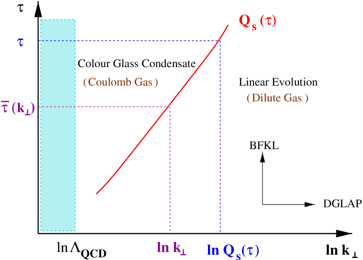
5.4 Low–$k_{\perp}\,$: Coulomb gas and gluon saturation

We finally turn to the most interesting physical regime, that of the non-linear physics at small transverse momenta $k_{\perp}\ll Q_{s}(\tau)$ (with $k_{\perp}\gg\Lambda_{QCD}$, though), whose understanding was a main motivation for all the previous developments.

Within the effective theory, the low-momentum modes of the colour source are described by the weight function ${\cal W}_{\tau}^{\,{\rm low}}$, eq. (5.39), which is equivalently rewritten as (cf. Fig.  18):

$${\cal W}_{\tau}^{\,{\rm low}}[\rho]\,=\,{\cal N}_{\tau}\,{\rm exp}\!\Biggl{\{}-\,{\pi\over 2}\int\limits^{Q_{s}^{2}(\tau)}{d^{2}k_{\perp}\over(2\pi)^{2}}\!\int\limits_{\bar{\tau}(k_{\perp})}^{\tau}\!d{\rm y}\,\frac{\rho_{\rm y}^{a}(k_{\perp})\rho_{\rm y}^{a}(-k_{\perp})}{k_{\perp}^{2}}\Bigg{\}},\,\,\,\,\,$$ (5.50)

with $\bar{\tau}(k_{\perp})=$ the rapidity at which the saturation momentum is equal to $k_{\perp}\,$:

$$Q_{s}^{2}(\bar{\tau}(k_{\perp}))\,=\,k_{\perp}^{2}\,.$$ (5.51)

There are several noteworthy features about eq. (5.50) :

i) This describes a Coulomb gas, i.e., a system of colour charges interacting via long-range Coulomb forces. The colour source $\rho_{\rm y}^{a}(x_{\perp})$ at $x_{\perp}$ feels the Coulomb field $\alpha_{\rm y}^{a}(x_{\perp})$ created at $x_{\perp}$ by all the other sources:

$$\int_{k_{\perp}}\!\!\frac{\rho_{\rm y}^{a}(k_{\perp})\rho_{\rm y}^{a}(-k_{\perp})}{k_{\perp}^{2}}=\!\int_{x_{\perp},y_{\perp}}\!\!\!\rho_{\rm y}^{a}(x_{\perp})\langle x_{\perp}|\,\frac{1}{-\nabla^{2}_{\perp}}\,|y_{\perp}\rangle\rho_{\rm y}^{a}(y_{\perp})=\!\int_{x_{\perp}}\!\!\rho_{\rm y}^{a}(x_{\perp})\alpha_{\rm y}^{a}(x_{\perp}).$$

The fact that the charge-charge correlator appears to vanish when $k_{\perp}\to 0$ is in agreement with gauge symmetry: The colour source $\rho_{\rm y}^{a}(k_{\perp})$ at low $k_{\perp}$ is an induced source, whose global strength must vanish:

$$\langle{\cal Q}^{2}\rangle\equiv\int_{x_{\perp},y_{\perp}}\!\!\int_{{\rm y},{\rm y^{\prime}}}\langle\rho_{\rm y}^{a}(x_{\perp})\rho_{\rm y^{\prime}}^{a}(y_{\perp})\rangle\propto\langle\rho_{\rm y}^{a}(k_{\perp})\rho_{\rm y}^{a}(-k_{\perp})\rangle\Big{|}_{k_{\perp}=0}=0.$$ (5.52)

ii) The colour charge correlations are local in rapidity : the Coulomb forces couple only sources located in the same layer of y (or $x^{-}$). At low–$k_{\perp}$, this property is not just an artifact of the MFA, but rather has a deep physical meaning: In the quantum evolution, the colour sources at different rapidities get correlated with each other because of the presence of Wilson lines in the evolution Hamiltonian (4.1). But these correlations are washed out on a large scale $r_{\perp}\gg 1/Q_{s}(\tau)$, on which the Wilson lines average to zero. In particular, this explains why the width $\propto k_{\perp}^{2}$ of the Gaussian (5.50) is independent of the initial conditions at ${\tau}\simeq 0$. (By contrast, at high momenta, the width $\lambda_{\rm y}(k_{\perp})=\partial\mu_{\rm y}(k_{\perp})/\partial{\rm y}$ in eq. (5.40) is sensitive to the initial conditions, since determined by solving eq. (5.32).)

iii) According to eq. (5.50), the low-momentum modes of $\rho$ are uniformly distributed in rapidity, within the interval $\bar{\tau}(k_{\perp})<{\rm y}<\tau$. It follows that the integrated quantity:

$$\mu_{\tau}(k_{\perp})=\int\limits_{\bar{\tau}(k_{\perp})}^{\tau}\!d{\rm y\,}\,\frac{k_{\perp}^{2}}{\pi}\,=\Big{(}\tau-\bar{\tau}(k_{\perp})\Big{)}\frac{k_{\perp}^{2}}{\pi}\,,$$ (5.53)

which measures the density of sources (with given $k_{\perp}$) in the transverse plane, grows only linearly with $\tau$, that is, logarithmically with the energy. This is to be contrasted with the strong, quasi-exponential, increase of $\mu_{\tau}(k_{\perp})$ in the high-momentum regime (cf. eqs. (5.45) and (5.46)). We conclude that, at low momenta $k_{\perp}\ll Q_{s}(\tau)$, the colour sources saturate, because of the strong non-linear effects in the quantum evolution.

iv) The saturated sources form the outermost layers of the hadron in the longitudinal direction: for given $k_{\perp}$, they are located at $x^{-}\geq x^{-}_{0}{\rm e}^{\bar{\tau}(k_{\perp})}$. In particular,

$$\tau\,-\,\bar{\tau}(k_{\perp})\,\simeq\,{1\over 4\bar{\alpha}_{s}}\,\ln{Q_{s}^{2}(\tau)\over k_{\perp}^{2}}\,,$$ (5.54)

is the longitudinal extent of the saturated part of the hadron, in units of rapidity (for modes with tranverse momentum $k_{\perp}$). In writing (5.54), we have used the DLA estimate (5.48) for the $\tau$-dependence of the saturation scale.

v) Note the factor $1/\alpha_{s}$ in the r.h.s. of (5.54); this implies that, at saturation, the integrated charge density $\rho^{a}(x_{\perp})$ has typically large amplitudes: $\bar{\rho}\sim\sqrt{\langle\rho\rho\rangle}\sim 1/g$. The same is therefore true for the COV-gauge field $\alpha^{a}(x_{\perp})$ : $\bar{\alpha}\sim 1/g$.

Since the colour sources at low–$k_{\perp}$ are saturated, there should be no surprise that the gluons emitted by these sources are saturated as well, and this independently of their mutual interactions (i.e., of the non-linear effects in the classical Yang-Mills equations). Indeed, a quasi-Abelian calculation of the gluon distribution, based on the linearized solution ${\cal F}^{+j}(k)\approx(ik^{j}/k_{\perp}^{2})\rho$, yields the following gluon density (cf. eqs. (5.42) and eq. (5.53)) :

$${\cal N}_{\tau}(k_{\perp})\,\simeq\,{N_{c}^{2}-1\over 4\pi^{4}c}\,\Bigl{(}\tau-\bar{\tau}(k_{\perp})\Bigr{)}\,\simeq\,{N^{2}_{c}-1\over 16\pi^{4}c}\,{1\over\bar{\alpha}_{s}}\,\ln{Q_{s}^{2}(\tau)\over k_{\perp}^{2}}\,,$$ (5.55)

which already exhibits saturation ! In fact, as argued in Refs. [10], the only effect of the non-linearities in the classical Yang-Mills equations in this low–$k_{\perp}$ regime is to modify the overall normalization of the linear-order result. In anticipation of this, we have inserted in eq. (5.55) a corrective factor $c$, which cannot be accurately determined in the present approximations (since sensitive to the physics around $Q_{s}$), but should be smaller than one (although not much smaller).

Note the striking similarity between eq. (5.55) and the corresponding prediction (2.71) of the classical MV model. Despite of the differences in the physical mechanism leading to saturation — non-linear quantum evolution for eq. (5.55), as opposed to non-linear classical dynamics for eq. (2.71) —, the final results look very much the same. So, the earlier discussion of eq. (2.71) can be immediately adapted to eq. (5.55), after replacing $A\to s$ : Eq. (5.55) shows marginal saturation (in the sense of a logarithmic increase only) with both $s$ and $1/k_{\perp}^{2}$, with a typical amplitude of order $1/\alpha_{s}$. This is illustrated in Fig. 19, which should be compared to Fig. 13. (The high–$k_{\perp}$ behaviour in Fig. 19 is taken from eq. (5.42).)

Figure 19: The gluon phase-density ${\cal N}_{\tau}(k_{\perp})$ in the effective theory plotted as a function of $k_{\perp}$ for two values of $\tau=\ln(1/{\rm x})$.

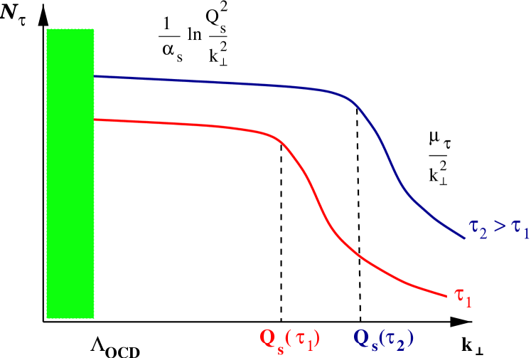
Aside from saturation, eq. (5.55) has also other important consequences, which all reflect the proportionality to the rapidity window $\tau-\bar{\tau}(k_{\perp})$, eq. (5.54):

a) Scaling. The gluon density at saturation depends upon the energy $s$ and the transverse momentum $k_{\perp}$ only via the scaling variable

$${\cal T}\equiv{Q_{s}^{2}(\tau)/k_{\perp}^{2}}\,.$$ (5.56)

A similar scaling is observed in the solutions to the Kovchegov equation [19, 56, 58]. As mentioned in the Introduction, such a scaling has been actually observed in DIS at HERA [17].

b) Universality. Eq. (5.55) is only weakly sensitive — via its logarithmic dependence upon the saturation scale — to the initial conditions for quantum evolution, and therefore to the specific properties of the hadron under consideration (e.g., its size and atomic number). Thus, eq. (5.55) not only provides arguments in the favour of hadron universality at high energy, but also predicts what should be the pattern of its violation.

The gluon distribution ${\rm x}G({\rm x},Q^{2})$ at $Q^{2}\ll Q_{s}^{2}(\tau)$ is immediately obtained by integration in eq. (5.55):

$${\rm x}G({\rm x},Q^{2}) \simeq {N^{2}_{c}-1\over 16\pi^{3}c}\,{1\over\bar{\alpha}_{s}}\,\,\pi R^{2}\int\limits^{Q^{2}}_{0}{dk_{\perp}^{2}}\,\ln{Q_{s}^{2}(\tau)\over k_{\perp}^{2}}$$ (5.57)

$$= {N^{2}_{c}-1\over 16\pi^{2}c}\,{1\over\bar{\alpha}_{s}}\,R^{2}Q^{2}\left[\ln(Q_{s}^{2}(\tau)/Q^{2})+1\right].$$

Note that, since $\mu_{\tau}(k_{\perp})\sim k_{\perp}^{2}$ in the saturation regime (cf. eq. (5.53)), the above integral is almost insensitive to the soft modes $k_{\perp}\mathrel{\hbox to0.0pt{\raise 2.20013pt\hbox{$<$}\hss}{\lower 2.20013pt\hbox{$\sim$}}}\Lambda_{QCD}$. This has allowed us to extend the integration down to $k_{\perp}=0$ without loss of accuracy. As anticipated, the phenomenon of saturation reduces the sensitivity of physical quantities to the infrared gauge fields, thus making the weak coupling expansion reliable. (In Ref. [58] a similar conclusion is drawn on the basis of Kovchegov equation.) If extrapolated up to $Q\sim Q_{s}$, eq. (5.57) yields

$${\rm x}G({\rm x},Q_{s}^{2}(\tau))\,\simeq\,{N^{2}_{c}-1\over 16\pi^{2}c}\,{1\over\bar{\alpha}_{s}}\,R^{2}Q_{s}^{2}(\tau),$$ (5.58)

in rough agreement with the corresponding extrapolation from the high momentum regime, eq. (5.47). Eq. (5.58) gives also the contribution of the saturated modes to the gluon distribution at momenta $Q>Q_{s}(\tau)$. But for very high momenta, $Q\gg Q_{s}(\tau)$, the dominant contribution comes form the hard modes ($Q_{s}\ll k_{\perp}\mathrel{\hbox to0.0pt{\raise 2.20013pt\hbox{$<$}\hss}{\lower 2.20013pt\hbox{$\sim$}}}Q$), and is given by eq. (5.43).

As a final application, let us compute the 2-point function $S_{\tau}(r_{\perp})$ of the Wilson lines for large distances $r_{\perp}\gg 1/Q_{s}(\tau)$. This is interesting for at least two reasons: It shows how the unitarity limit is reached for the scattering of a large colour dipole off the hadron, and it allows us to check a posteriori the consistency of the “random phase approximation” that we have used at low $k_{\perp}$.

To this aim, we rewrite eq. (5.27) as

$$S_{\tau}(r_{\perp})\simeq{\rm exp}\Bigg{\{}-\frac{g^{2}N_{c}}{\pi}\int\limits_{-\infty}^{\tau}d{\rm y}\int\limits^{Q_{s}({\rm y})}{d^{2}p_{\perp}\over(2\pi)^{2}}\,\frac{1}{p_{\perp}^{2}}\,\Bigl{[}1-{\rm e}^{ip_{\perp}\cdot r_{\perp}}\Bigr{]}\Bigg{\}},$$ (5.59)

where we have anticipated that the main contribution comes from the saturated modes, for which $\gamma_{\tau}=1/(\pi p_{\perp}^{2})$, cf. eq. (5.36). The integral over $p_{\perp}$ is now infrared finite (as opposed to the MV model: compare to eq. (2.64)), and to leading log accuracy can be evaluated as:

$$\int\limits^{Q_{s}({\rm y})}{d^{2}p_{\perp}\over(2\pi)^{2}}\,\frac{1}{p_{\perp}^{2}}\,\Bigl{[}1-{\rm e}^{ip_{\perp}\cdot r_{\perp}}\Bigr{]}\,\simeq\,\theta({\rm y}-\bar{\tau}(r_{\perp}))\,{1\over 4\pi}\ln\Bigl{(}Q_{s}^{2}({\rm y})r_{\perp}^{2}\Bigr{)}.$$ (5.60)

The result can be understood as follows: as long as $1/r_{\perp}\gg Q_{s}({\rm y})$, or ${\rm y}<\bar{\tau}(r_{\perp})$, ${\rm e}^{ip_{\perp}\cdot r_{\perp}}\approx 1$, and the integral vanishes. Bur for ${\rm y}>\bar{\tau}(r_{\perp})$, or $1/r_{\perp}\ll Q_{s}({\rm y})$, the integrals corresponding to the two terms in the brackets are cut off at different ultraviolet scales: $Q_{s}({\rm y})$ for the first term, and $1/r_{\perp}$ for the second one. Their difference gives the log in the r.h.s. By also using $\ln(Q_{s}^{2}({\rm y})r_{\perp}^{2})=4\bar{\alpha}_{s}({\rm y}-\bar{\tau}(r_{\perp}))$, cf. eq. (5.54), and performing the integral over y, we finally deduce:

$$S_{\tau}(r_{\perp})\simeq\,{\rm exp}\Bigl{\{}-2\bar{\alpha}_{s}^{2}(\tau-\bar{\tau}(r_{\perp}))^{2}\Bigr{\}}\,=\,{\rm exp}\bigg{\{}-{1\over 8}\Bigl{[}\ln(Q_{s}^{2}(\tau)r_{\perp}^{2})\Bigr{]}^{2}\bigg{\}},$$ (5.61)

which coincides with the result obtained from the Kovchegov equation [19, 14]. Eq. (5.61) shows that the correlator of the Wilson lines is rapidly decreasing when $Q_{s}^{2}(\tau)r_{\perp}^{2}\gg 1$, so that the RPA is indeed justified, at least as a mean field approximation.

More details and further applications of the mean field approximation will be presented in Ref. [57], where the results obtained in this way will be also compared to the corresponding predictions of the Kovchegov equation. It would be also interesting (especially in view of applications to phenomenology) to take into account the transverse inhomogeneity of the hadron (i.e., the dependence upon the impact parameter in the transverse plane). This can be done already in the framework of the MFA, but, more generally, it would be important to understand the limitations of the latter, and to be able to solve the complete RGE. This might be done, for instance, via numerical simulations on a lattice.

6 Acknowledgments

We would like to thank our colleagues Alejandro Ayala-Mercado, Jean-Paul Blaizot, Elena Ferreiro, Kazunori Itakura, Dima Kharzeev, Yuri Kovchegov, Alex Kovner, Jamal Jalilian-Marian, Genya Levin, Al Mueller, Robi Peschanski, Raju Venugopalan and Heribert Weigert with whom many of the ideas presented in these lectures were developed, or discussed. We particularly thank Kazunori Itakura and Michaela Oswald for a careful and critical reading of the manuscript.

This manuscript has been authorized under Contract No. DE-AC02-98H10886 with the U. S. Department of Energy.

References

- [1] G. Sterman, An Introduction to Quantum Field Theory, Cambridge University Press, Cambridge, 1993; M.E. Peskin and D.V. Schroeder, An Introduction to Quantum Field Theory, Addison-Wesley, New York, 1995; R.K. Ellis, W.J. Stirling and B.R. Webber, QCD and Collider Physics, Cambridge University Press, Cambridge, 1996.
- [2] J. Breitweg et. al., Eur. Phys. J. 67, 609 (1999) and references therein.
- [3] L.N. Lipatov, Sov. J. Nucl. Phys. 23 (1976), 338; E.A. Kuraev, L.N. Lipatov and V.S. Fadin, Sov. Phys. JETP 45 (1977), 199; Ya.Ya. Balitsky and L.N. Lipatov, Sov. J. Nucl. Phys. 28 (1978), 822.
- [4] J.R. Forshaw and D.A. Ross, Quantum Chromodynamics and the Pomeron, Cambridge University Press, Cambridge, 1997.
- [5] V.N. Gribov and L.N. Lipatov, Sov. Journ. Nucl. Phys. 15 (1972), 438; G. Altarelli and G. Parisi, Nucl. Phys. B126 (1977), 298; Yu. L. Dokshitzer, Sov. Phys. JETP 46 (1977), 641. See also Yu. L. Dokshitzer, V. A. Khoze, A. H. Mueller, and S.I. Troyan, “Basics of Perturbative QCD” (Editions Frontières, Gif-sur-Yvette, 1991).
- [6] L. V. Gribov, E. M. Levin, and M. G. Ryskin, Phys. Rept. 100 (1983) 1.
- [7] A. H. Mueller and Jian-wei Qiu, Nucl. Phys. B268 (1986) 427.
- [8] L.McLerran and R. Venugopalan, Phys. Rev. D49 (1994) 2233; ibid. 49 (1994) 3352; ibid. 50 (1994) 2225.
- [9] A. H. Mueller, Nucl. Phys. B558 (1999), 285.
- [10] E. Iancu and L. McLerran, Phys. Lett. B510 (2001) 145.
- [11] A. H. Mueller, Small-x Physics, High Parton Densities and Parton Saturation in QCD, hep-ph/9911289. Published in Lisbon 1999, QCD: Perturbative or nonperturbative?, pp. 180-209.
- [12] L. McLerran, The color glass condensate and small x physics: 4 lectures, Lectures given at 40th Internationale Universitatswochen fuer Theoretische Physik: Dense Matter (IUKT 40), Schladming, Austria, 3-10 Mar 2001, hep-ph/0104285.
- [13] E. Levin, Saturation at low x, hep-ph/0105205.
- [14] A. H. Mueller, Parton Saturation-An Overview, Cargese lectures, hep-ph/0111244 (this volume).
- [15] J.-P. Blaizot and E. Iancu, The quark-gluon plasma: Collective dynamics and hard thermal loops, hep-ph/0101103, Physics Reports (to appear).
- [16] J.-P. Blaizot and A. H. Mueller, Nucl. Phys. B289 (1987) 847.
- [17] A. M. Stasto, K. Golec-Biernat and J. Kwieczinski, Phys. Rev. Lett., 86, 596 (2001).
- [18] K. Golec-Biernat and M. Wüsthoff, Phys. Rev. D59 (1999), 014017; ibid. D60 (1999) 114023; Eur. Phys. J. C20 (2001) 313.
- [19] E. Levin and K. Tuchin, Nucl. Phys. B573 (2000) 833; Nucl.Phys. A691 (2001) 779; Nucl.Phys. A693 (2001) 787.
- [20] A. Krasnitz, R. Venugopalan, Phys. Rev. Lett. 84 (2000) 4309; ibid. 86 (2001) 1717; A. Krasnitz, Y. Nara, and R. Venugopalan, Phys. Rev. Lett. 87 (2001) 192302.
- [21] A. Kovner, L. McLerran and H. Weigert, Phys. Rev. D52 (1995) 3809; ibid. 6231.
- [22] R. Baier, A.H. Mueller, D. Schiff and D.T. Son, Phys. Lett. B502 (2001) 51.
- [23] See, e.g., the proceedings of 15th International Conference on Ultrarelativistic Nucleus-Nucleus Collisions (QM2001), Stony Brook, New York, 15-20 Jan 2001. Published in Nucl. Phys. A698 (2002).
- [24] D. Kharzeev, M. Nardi, Phys. Lett. B507 (2001) 121.
- [25] D. E. Kharzeev, E. Levin, Phys. Lett. B523 (2001) 79.
- [26] L. McLerran, J. Schaffner-Bielich, Phys. Lett. B514 (2001) 29; J. Schaffner-Bielich, D. Kharzeev, L. McLerran and R. Venugopalan, nucl-th/0108048.
- [27] F. Gelis and A. Peshier, Nucl. Phys. A697 (2002) 879; hep-ph/0111227.
- [28] R. Venugopalan, Deeply inelastic scattering off nuclei at RHIC, hep-ph/0102087.
- [29] A. Dumitru, L. McLerran, How protons shatter colored glass, hep-ph/0105268.
- [30] Yu. V. Kovchegov, Nucl.Phys. A692 (2001) 557; Phys.Rev. D64 (2001) 114016.
- [31] D. E. Kharzeev, Yu. V. Kovchegov, and E. Levin, Nucl. Phys. A699 (2002) 745.
- [32] Yu.V. Kovchegov, Phys. Rev. D54 (1996), 5463; Phys. Rev. D55 (1997), 5445.
- [33] J. Jalilian-Marian, A. Kovner, L. McLerran and H. Weigert, Phys. Rev. D55 (1997), 5414.
- [34] Yu.V. Kovchegov and A.H. Mueller, Nucl. Phys. B529 (1998), 451.
- [35] C. S. Lam and G. Mahlon, Phys. Rev. D62 (2000) 114023; ibid. D64 (2001) 016004.
- [36] J. Jalilian-Marian, A. Kovner, A. Leonidov and H. Weigert, Nucl. Phys. B504 (1997), 415; Phys. Rev. D59 (1999), 014014.
- [37] E. Iancu, A. Leonidov and L. McLerran, Nucl. Phys. A692 (2001), 583; Phys. Lett. B510 (2001) 133; E. Ferreiro, E. Iancu, A. Leonidov and L. McLerran, hep-ph/0109115.
- [38] R. Venugopalan, Classical methods in DIS and nuclear scattering at small x, Lectures at the XXXIX Cracow School of Theoretical Physics, Zakopane, Poland, May29th-June8th, 1999. Published in Acta Phys. Polon. B30 (1999) 3731.
- [39] J.B. Kogut and D.E. Soper, Phys.Rev. D1 (1970) 2901.
- [40] A. H. Mueller, Nucl. Phys. B335 (1990) 115.
- [41] N.N. Nikolaev and B.G. Zakharov, Z. Phys. C49 (1991) 607, ibid. C53 (1992) 331.
- [42] W. Buchmuller, M.F. McDermott and A. Hebecker, Nucl. Phys. B487 (1997) 283, Erratum-ibid. B500 (1997) 621; W. Buchmuller, T. Gehrmann, and A. Hebecker Nucl. Phys. B537 (1999) 477.
- [43] K. H. Fischer and J. A. Hertz, Spin glasses, Cambridge University Press, Cambridge, 1991.
- [44] I. Balitsky, Nucl. Phys. B463 (1996), 99; High-energy QCD and Wilson lines, hep-ph/0101042.
- [45] Yu. V. Kovchegov, Phys. Rev. D60 (1999), 034008; ibid. D61 (2000), 074018.
- [46] A. H. Mueller, Nucl. Phys. B415 (1994), 373; ibid. B437 (1995), 107.
- [47] H. Weigert, Unitarity at small Bjorken x, hep-ph/0004044.
- [48] A. H. Mueller, Phys. Lett. B523 (2001) 243.
- [49] A. Kovner, J. G. Milhano and H. Weigert, Phys. Rev. D62 (2000), 114005.
- [50] M. Braun, Eur. Phys. J. C16 (2000) 337; N. Armesto and M. Braun, ibid. C20 (2001) 517.
- [51] I. Balitsky and A.V. Belitsky, Nonlinear evolution in high-density QCD, hep-ph/0110158.
- [52] J.-P. Blaizot, E. Iancu and H. Weigert, in preparation.
- [53] I. Balitsky, Phys. Lett. B518 (2001) 235.
- [54] M. Lublinsky, E. Gotsman, E. Levin, and U. Maor, Nucl.Phys. A696 (2001) 851; E. Levin and M. Lublinsky, Nucl.Phys. A696 (2001) 833.
- [55] E. Levin and M. Lublinsky, Phys. Lett. B521 (2001) 233; Eur. Phys. J. C22 (2002) 647.
- [56] M. Lublinsky, Eur. Phys. J. C21 (2001) 513.
- [57] E. Iancu, K. Itakura, and L. McLerran, in preparation.
- [58] K. Golec-Biernat, L. Motyka, and A. M. Stasto, Diffusion into infra-red and unitarization of the BFKL pomeron, hep-ph/0110325.
-
[59]
G. Parisi, Statistical Field Theory, Addison-Wesley,
New York, 1988;
J. Zinn-Justin, Quantum field theory and critical phenomena, (International series of monographs on physics, 77), Clarendon, Oxford, 1989.