FERMILAB-PUB-02/040-T
BUHEP-02-15
hep-ph/0202255

Two Lectures on Technicolor

Abstract

These two lectures on technicolor and extended technicolor (ETC) were presented at l’Ecole de GIF at LAPP, Annecy-le-Vieux, France, in September 2001. In Lecture I, the motivation and structure of this theory of dynamical breaking of electroweak and flavor symmetries is summarized. The main phenomenological obstacles to this picture—flavor–changing neutral currents, precision electroweak measurements, and the large top–quark mass—are reviewed. Then, their proposed resolutions—walking technicolor and topcolor–assisted technicolor are discussed. In Lecture II, a scenario for CP violation is presented based on vacuum alignment for technifermions and quarks. It has the novel feature of CP–violating phases that are rational multiples of $\pi$ to better than one part in $10^{10}$ without fine–tuning of parameters. The scheme thereby avoids light axions and a massless up quark. The mixing of neutral mesons, the mechanism of top–quark mass generation, and the CP–violating parameters $\epsilon$ and $\sin(2\beta)$ strongly constrain the form of ETC–generated quark mass matrices.

I. INTRODUCTION TO TECHNICOLOR

“Faith” is a fine invention

When Gentlemen can see —

But Microscopes are prudent

In an Emergency.

— Emily Dickinson, 1860

I.1 The Motivation for Technicolor and Extended Technicolor

The elements of the standard model of elementary particles have been in place for more than 25 years now. These include the $SU(3)\otimes SU(2)\otimes U(1)$ gauge model of strong and electroweak interactions [4, 5]. And, they include the Higgs mechanism used to break spontaneously electroweak $SU(2)\otimes U(1)$ down to the $U(1)$ of electromagnetism [6]. In the standard model, couplings of the elementary Higgs scalar bosons also break explicitly quark and lepton chiral–flavor symmetries, giving them hard masses (i.e., mass terms that appear in the Lagrangian). In this quarter century, the standard model has stood up to the most stringent experimental tests [7, 8]. The only clear indications we have of physics beyond this framework are the existence of neutrino mixing and, presumably, masses (though some would say this physics is accommodated within the standard model); the enormous range of masses, about $10^{12}$, between the neutrinos and the top quark; the need for a new source of CP–violation to account for the baryon asymmetry of the universe; the likely presence of cold dark matter; and, possibly, a very small, but nonzero, cosmological constant. These hints are powerful. But they are also obscure, and they do not point unambiguously to any particular extension of the standard model.

In addition to these experimental facts, considerable theoretical discomfort and dissatisfaction with the standard model have dogged it from the beginning. All of it concerns the elementary Higgs boson picture of electroweak and flavor symmetry breaking—the cornerstone of the standard model. In particular:

1. Elementary Higgs models provide no dynamical explanation for electroweak symmetry breaking.

2. Elementary Higgs models are unnatural, requiring fine tuning of parameters to enormous precision.

3. Elementary Higgs models with grand unification have a hierarchy problem of widely different energy scales.

4. Elementary Higgs models are trivial.

5. Elementary Higgs models provide no insight to flavor physics.

In nonsupersymmetric Higgs models, there is no explanation why electroweak symmetry breaking occurs and why it has the energy scale of 1 TeV. The Higgs doublet self–interaction potential is $V(\phi)=\lambda\thinspace(\phi^{\dagger}\phi-v^{2})^{2}$, where $v$ is the vacuum expectation of the Higgs field $\phi$ provided that $v^{2}\geq 0$. Its experimental value is $v=2^{-1/4}G_{F}^{-1/2}=246\,{\rm GeV}$. But what dynamics makes $v^{2}>0$? What dynamics sets its magnitude? In supersymmetric Higgs models, the large top–quark Yukawa coupling can drive $v^{2}$ positive (by driving $M^{2}_{H}$ negative), but this just replaces one problem with another since we don’t know why the top’s Yukawa coupling is ${\cal O}(1)$. Furthermore, this electroweak symmetry breaking scenario requires the supersymmetric “mu–term” to be ${\cal O}(1\,{\rm TeV})$. Why that value?

Elementary Higgs boson models are unnatural. The Higgs boson’s mass, $M^{2}_{H}=2\lambda v^{2}$ is quadratically unstable against radiative corrections [9]. Thus, there is no natural reason why $M_{H}$ and $v$ should be much less than the energy scale at which the essential physics of the model changes, e.g., a unification scale or the Planck scale of $10^{16}\,{\rm TeV}$. To make $M_{H}$ very much less that $M_{P}$, say 1 TeV, the bare Higgs mass must be balanced against its radiative corrections to the fantastic precision of a part in $M^{2}_{P}/M^{2}_{H}\sim 10^{32}$.

In grand–unified Higgs boson models, supersymmetric or not, there are two very different scales of gauge symmetry breaking, the GUT scale of about $10^{16}\,{\rm GeV}$ and the electroweak scale of a few 100 GeV. This hierarchy is put in by hand, and must be maintained by unnaturally–fine tuning in ordinary Higgs models, or by the “set it and forget it” nonrenormalization feature of supersymmetry.

Next, taken at face value, elementary Higgs boson models are free field theories [10]. To a good approximation, the self–coupling $\lambda(\mu)$ of the minimal one–doublet Higgs boson at an energy scale $\mu$ is given by

$$\lambda(\mu)\cong{\lambda(\Lambda)\over{1+(24/16\pi^{2})\thinspace\lambda(\Lambda)\thinspace\log(\Lambda/\mu)}}\thinspace.$$ (1)

This coupling vanishes for all $\mu$ as the cutoff $\Lambda$ is taken to infinity, hence the description “trivial”. This feature persists in a general class of two–Higgs doublet models [11] and it is probably true of all Higgs models. Triviality really means that elementary–Higgs Lagrangians are meaningful only for scales $\mu$ below some cutoff $\Lambda_{\infty}$ at which new physics sets in. The larger the Higgs couplings are, the lower the scale $\Lambda_{\infty}$. This relationship translates into the so–called triviality bounds on Higgs masses. For the minimal model, the connection between $M_{H}$ and $\Lambda_{\infty}$ is

$$M_{H}(\Lambda_{\infty})\cong\sqrt{2\lambda(M_{H})}\thinspace v={2\pi v\over{\sqrt{3\log(\Lambda_{\infty}/M_{H})}}}\thinspace.$$ (2)

Clearly, the cutoff has to be greater than the Higgs mass for the effective theory to have some range of validity. From lattice–based arguments [10], $\Lambda_{\infty}\mathrel{\hbox to0.0pt{\raise 2.20013pt\hbox{$>$}\hss}{\lower 2.20013pt\hbox{$\sim$}}}2\pi M_{H}$. Since $v$ is fixed at 246 GeV in the minimal model, this implies the triviality bound $M_{H}\mathrel{\hbox to0.0pt{\raise 2.20013pt\hbox{$<$}\hss}{\lower 2.20013pt\hbox{$\sim$}}}700\,{\rm GeV}$. If the standard Higgs boson were to be found with a mass this large or larger, we would know for sure that additional new physics is lurking in the range of a few TeV. If the Higgs boson is light, less than 200–300 GeV, as it is expected to be in supersymmetric models, this transition to a more fundamental theory may be postponed until very high energy, but what lies up there worries us nonetheless.

Finally, in all elementary Higgs models, supersymmetric or not, every aspect of flavor is completely mysterious, from the primordial symmetry defining the number of quark and lepton generations to the bewildering patterns of flavor breaking. The presence of Higgs bosons has no connection to the existence of multiple and identical fermion generations. The flavor–symmetry breaking Yukawa couplings of Higgs bosons to fermions are arbitrary free parameters, put in by hand. As far as we know, this is a logically consistent state of affairs, and we may not understand flavor until we understand the physics of the Planck scale. I do not believe this. And, I cannot see how this problem, more pressing and immediate than any save electroweak symmetry breaking itself, can be so cavalierly set aside by those pursuing the “theory of everything”.

The dynamical approach to electroweak and flavor symmetry breaking known as technicolor (TC) [13, 14, 2] and extended technicolor (ETC) [15, 16] emerged in the late 1970s in response to these shortcomings of the standard model. This picture was motivated first of all by the premise that every fundamental energy scale should have a dynamical origin. Thus, the weak scale embodied in the Higgs vacuum expectation value $v=246\,{\rm GeV}$ should reflect the characteristic energy of a new strong interaction—technicolor—just as the pion decay constant $f_{\pi}=93\,{\rm MeV}$ reflects QCD’s scale $\Lambda_{QCD}\sim 200\,{\rm MeV}$. For this reason, I write $F_{\pi}=2^{-1/4}G_{F}^{-1/2}=246\,{\rm GeV}$ to emphasize that this quantity has a dynamical origin.

Technicolor, a gauge theory of fermions with no elementary scalars, is modeled on the precedent of QCD: The electroweak assignments of quarks to left–handed doublets and right–handed singlets prevent their bare mass terms. If there are no elementary Higgses to couple to, quarks have a large chiral symmetry, $SU(6)_{L}\otimes SU(6)_{R}$ for three generations. This symmetry is spontaneously broken to the diagonal (vectorial) $SU(6)$ subgroup when the QCD gauge coupling grows strong near $\Lambda_{QCD}$. This produces 35 massless Goldstone bosons, the “pions”. According to the Higgs mechanism—whose operation requires no elementary scalar bosons [17]—this yields weak boson masses of $M_{W}=M_{Z}\cos\theta_{W}={\textstyle{{1\over{2}}}}\sqrt{3}gf_{\pi}\simeq 50\,{\rm MeV}$ [13]. These masses are 1600 times too small, but they do have the right ratio. Suppose, then, that there are fermions belonging to a complex representation of a new gauge group, technicolor (taken to be $SU(N_{TC})$), whose coupling $\alpha_{TC}$ becomes strong at $\Lambda_{TC}=100$s of GeV. If, like quarks, technifermions form left–handed doublets and right–handed singlets under $SU(2)\otimes U(1)$, then they have no bare masses. When $\alpha_{TC}$ becomes strong, the technifermions’ chiral symmetry is spontaneously broken, Goldstone bosons appear, three of them become the longitudinal components of $W^{\pm}$ and $Z^{0}$, and their masses are $M_{W}=M_{Z}\cos\theta_{W}={\textstyle{{1\over{2}}}}gF_{\pi}$. Here, $F_{\pi}\sim\Lambda_{TC}$ is the decay constant of the linear combination of the absorbed “technipions”.

Technicolor, like QCD, is asymptotically free. This solves in one stroke the naturalness, hierarchy, and triviality problems! The mass of all ground–state technihadrons, including Higgs–like scalars (though that language is neither accurate nor useful in technicolor) is of order $\Lambda_{TC}$ or less. There are no large renormalizations of bound state masses, hence no fine tuning of parameters. If the technicolor gauge symmetry is embedded at a very high energy $\Lambda$ in some grand unified gauge group with a relatively weak coupling, then the characteristic energy scale $\Lambda_{TC}$—where the coupling $\alpha_{TC}$ becomes strong enough to trigger chiral symmetry breaking—is naturally exponentially smaller than $\Lambda$. Finally, asymptotically free field theories are nontrivial. A minus sign in the denominator of the analog of Eq. (1) for $\alpha_{TC}(\mu)$ prevents one from concluding that it tends to zero for all $\mu$ as the cutoff is taken to infinity. No other scenario for the physics of the TeV scale solves these problems so neatly. Period.

Technicolor alone does not address the flavor problem. It does not tell us why there are multiple generations and it does not provide explicit breaking of quark and lepton chiral symmetries. Something must play the role of Higgs bosons to communicate electroweak symmetry breaking to quarks and leptons. Furthermore, in all but the minimal TC model with just one doublet of technifermions, there are Goldstone bosons, technipions $\pi_{T}$, in addition to $W_{L}^{\pm}$ and $Z_{L}^{0}$. These must be given mass and their masses must be more than 50–100 GeV for them to have escaped detection. Extended technicolor (ETC) was invented to address all these aspects of flavor physics [15]. It was also motivated by the desire to make flavor understandable at energies well below the GUT scale solely in terms of gauge dynamics of the kind that worked so neatly for electroweak symmetry breaking, namely, technicolor. Let me repeat: the ETC approach is based on the gauge dynamics of fermions only. There can be no elementary scalar fields to lead us into the difficulties technicolor itself was invented to escape.

I.2 Dynamical Basics

In extended technicolor, ordinary $SU(3)$ color, $SU(N_{TC})$ technicolor, and flavor symmetries are unified into the ETC gauge group, $G_{ETC}$. We then understand flavor, color, and technicolor as subsets of the quantum numbers of extended technicolor. Technicolor and color are exact gauge symmetries. Flavor gauge symmetries are broken at one or more high energy scales $\Lambda_{ETC}\simeq M_{ETC}/g_{ETC}$ where $M_{ETC}$ is a typical flavor gauge boson mass.

In these lectures, I assume that $G_{ETC}$ commutes with electroweak $SU(2)$. In this case, it must not commute with electroweak $U(1)$, i.e., some part of that $U(1)$ must be contained in $G_{ETC}$. Otherwise, there will be very light pseudoGoldstone bosons which behave like classical axions and are ruled out experimentally [15, 18]. More generally, all fermions—technifermions, quarks, and leptons—must form no more than four irreducible ETC representations: two equivalent ones for left–handed up and down–type fermions and two inequivalent ones for right–handed up and down fermions (so that up and down mass matrices are not identical). In other words, ETC interactions explicitly break all global flavor symmetries so that there are no very light pseudoGoldstone bosons or fermions.

The energy scale of ETC gauge symmetry breaking into $SU(3)\otimes SU(N_{TC})$ is high, well above the TC scale of 0.1–1.0 TeV. The broken gauge interactions, mediated by massive ETC boson exchange, give mass to quarks and leptons by connecting them to technifermions (Figure 1a). They give mass to technipions by connecting technifermions to each other (Figure 1b).

The graphs in Figure 1 are convergent: The changes in chirality imply insertions on the technifermion lines of the momentum–dependent dynamical mass, $\Sigma(p)$. This function falls off as $1/p^{2}\thinspace(\log(p/\Lambda_{TC}))^{c}$ in an asymptotically free theory at weak coupling and, in any case, at least as fast as $1/p$ [19, 20]. For such a power law, the dominant momentum running around the loop is ${\cal O}(M_{ETC})$ (extending down to $\Lambda_{TC}$ for a $1/p^{2}$ falloff of $\Sigma$). Then, the operator product expansion tells us that the generic quark or lepton mass and technipion mass are given by the expressions

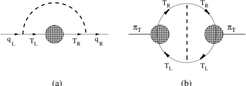
Figure 1: Graphs for ETC generation of masses for (a) quarks and leptons and (b) technipions. The dashed line is a massive ETC gauge boson. Higher–order technicolor gluon exchanges are not indicated; from Ref. [15].

$$m_{q}(M_{ETC})\simeq m_{\ell}(M_{ETC})\simeq 2{g_{ETC}^{2}\over{M_{ETC}^{2}}}\langle\bar{T}_{L}T_{R}\rangle_{ETC}\thinspace;$$ (3)

$$F^{2}_{T}M^{2}_{\pi_{T}}\simeq 2\thinspace{g^{2}_{ETC}\over{M^{2}_{ETC}}}\thinspace\langle\bar{T}_{L}T_{R}\bar{T}_{R}T_{L}\rangle_{ETC}\thinspace.$$ (4)

Here, $m_{q}(M_{ETC})$ is the quark mass renormalized at $M_{ETC}$. It is a hard mass in that it scales like one (i.e., logarithmically) for energies below $M_{ETC}$. Above that, it falls off more rapidly, like $\Sigma(p)$. The technipion decay constant $F_{T}=F_{\pi}/\sqrt{N}$ in TC models containing $N$ identical electroweak doublets of color–singlet technifermions. The vacuum expectation values $\langle\bar{T}_{L}T_{R}\rangle_{ETC}$ and $\langle\bar{T}_{L}T_{R}\bar{T}_{R}T_{L}\rangle_{ETC}$ are the bilinear and quadrilinear technifermion condensates renormalized at $M_{ETC}$. The bilinear condensate is related to the one renormalized at $\Lambda_{TC}$, expected by scaling from QCD to be

$$\langle\bar{T}_{L}T_{R}\rangle_{TC}={\textstyle{{1\over{2}}}}{\langle\bar{T}T\rangle}_{TC}\simeq 2\pi F^{3}_{T}\thinspace,$$ (5)

by the equation

$${\langle\bar{T}T\rangle}_{ETC}={\langle\bar{T}T\rangle}_{TC}\thinspace\exp\left(\int_{\Lambda_{TC}}^{M_{ETC}}\thinspace{d\mu\over{\mu}}\thinspace\gamma_{m}(\mu)\right)\thinspace.$$ (6)

The anomalous dimension $\gamma_{m}$ of the operator $\bar{T}T$ is given in perturbation theory by

$$\gamma_{m}(\mu)={3C_{2}(R)\over{2\pi}}\alpha_{TC}(\mu)+O(\alpha_{TC}^{2})\thinspace,$$ (7)

where $C_{2}(R)$ is the quadratic Casimir of the technifermion $SU(N_{TC})$–representation $R$. For the fundamental representation of $SU(N_{TC})$, it is given by $C_{2}(N_{TC})=(N_{TC}^{2}-1)/2N_{TC}$. Finally, in the large–$N_{TC}$ approximation (which will be questionable in the walking technicolor theories we discuss later, but which we adopt anyway for rough estimates)

$$\langle\bar{T}_{L}T_{R}\bar{T}_{R}T_{L}\rangle_{ETC}\simeq\langle\bar{T}_{L}T_{R}\rangle_{ETC}\thinspace\langle\bar{T}_{R}T_{L}\rangle_{ETC}={\textstyle{{1\over{4}}}}{\langle\bar{T}T\rangle}_{ETC}^{2}\thinspace.$$ (8)

We can estimate $M_{ETC}$ and $M_{\pi_{T}}$ if we assume that technicolor is QCD–like [15]. In that case, its asymptotic freedom sets in quickly (or “precociously”) at energies above $\Lambda_{TC}$ and, so, $\gamma_{m}(\mu)\ll 1$ for $\mu$ greater than a few times $\Lambda_{TC}$. Then Eq. (5) applies to ${\langle\bar{T}T\rangle}_{ETC}$ as well. For $N$ technidoublets, the ETC scale required to generate $m_{q}(M_{ETC})\simeq 1\,{\rm GeV}$ is

$$\Lambda_{ETC}\equiv{M_{ETC}\over{g_{ETC}}}\simeq\sqrt{{4\pi F_{\pi}^{3}\over{m_{q}N^{3/2}}}}\simeq{14\,{\rm TeV}\over{N^{3/4}}}\thinspace.$$ (9)

This is pretty low, but the estimate is rough. The typical technipion mass implied by this ETC scale is

$$M_{\pi_{T}}\simeq{{\langle\bar{T}T\rangle}_{TC}\over{\sqrt{2}\Lambda_{ETC}F_{T}}}\simeq{40\,{\rm GeV}\over{N^{1/4}}}\thinspace.$$ (10)

Finally, some phenomenological basics: In any model of technicolor, one expects bound technihadrons with a spectrum of mesons paralleling what we see in QCD. The principal targets of collider experiments are the spin–zero technipions and spin–one isovector technirhos and isoscalar techniomegas. In the minimal one–technidoublet model ($T=(T_{U},T_{D})$), the three technipions are the longitudinal components $W_{L}$ of the massive weak gauge bosons. Susskind pointed out that the analog of the QCD decay $\rho\rightarrow\pi\pi$ is $\rho_{T}\rightarrow W_{L}W_{L}$ [13]. In the limit that $M_{\rho_{T}}\gg M_{W,Z}$, the equivalence theorem states that the amplitude for $\rho_{T}\rightarrow W_{L}W_{L}$ has the same form as the one for $\rho\rightarrow\pi\pi$. If we scale technicolor from QCD and use large–$N_{TC}$ arguments, the strength of this amplitude is $g_{\rho_{T}}\equiv\sqrt{4\pi\alpha_{\rho_{T}}}\simeq\sqrt{4\pi(3/N_{TC})\alpha_{\rho}}$ where $\alpha_{\rho}=2.91$. The $\rho_{T}$ mass and decay rate are [21]:

$$M_{\rho_{T}}=\sqrt{{3\over{N_{TC}}}}\thinspace{F_{\pi}\over{f_{\pi}}}M_{\rho}\simeq 2\sqrt{{3\over{N_{TC}}}}\,{\rm TeV}\thinspace,$$

$$\Gamma(\rho_{T}\rightarrow W_{L}W_{L})={2\alpha_{\rho_{T}}p_{W}^{3}\over{3M^{2}_{\rho_{T}}}}\simeq 500\left({3\over{N_{TC}}}\right)^{3/2}\,{\rm GeV}\thinspace.$$ (11)

In the minimal model, a very high energy machine, such as the ill–fated Superconducting Super Collider or the $200\,{\rm TeV}$ Very Large Hadron Collider or a $2\,{\rm TeV}$ Linear Collider is needed to discover the lightest technihadrons. In nonminimal models, where $N\geq 2$, the signatures of technicolor ought to be accessible at the Large Hadron Collider (LHC) and at a comparable lepton collider. As discussed in Ref. [1], the many technifermions needed for walking technicolor and topcolor–assisted technicolor (see below) mean that signatures are likely to be within reach of the Tevatron Collider in Run II! 

I.3 Dynamical Perils

Technicolor and extended technicolor are challenged by a number of phenomenological hurdles, but the most widely cited causes of the “death of technicolor” (prematurely announced, like Mark Twain’s) are flavor–changing neutral current interactions (FCNC) [15, 24], precision measurements of electroweak quantities (STU) [25], and the large mass of the top quark. We discuss these in turn.

I.3.1 Flavor–Changing Neutral Currents

Extended technicolor interactions are expected to have flavor–changing neutral currents involving quarks and leptons. The reason is simple: Realistic quark mass matrices require ETC transitions between different flavors, $q\rightarrow T\rightarrow q^{\prime}$, or technifermion mixing so that $q\rightarrow T\rightarrow T^{\prime}\rightarrow q^{\prime}$. In the first case, there must be ETC currents of the form $\bar{q}^{\prime}_{L,R}\thinspace\gamma_{\mu}\thinspace T_{L,R}$ and $\bar{T}_{L,R}\thinspace\gamma_{\mu}\thinspace q_{L,R}$. Their commutator algebra includes the ETC currents $\bar{q}^{\prime}_{L,R}\thinspace\gamma_{\mu}\thinspace q_{L,R}$. In the second case, these currents may be generation conserving. Either way, ETC interactions necessarily produce $\bar{q}q\bar{q}q$ operators involving light quarks. Similarly, there will be $\bar{q}q\bar{\ell}\ell$ and $\bar{\ell}\ell\bar{\ell}\ell$ operators. Even if these interactions are electroweak–eigenstate conserving (or generation conserving), they will induce FCNC four–fermion operators after diagonalization of mass matrices and transformation to the mass–eigenstate basis. No satisfactory GIM mechanism has ever been found that eliminates these FCNC interactions [26].

The most stringent constraint on ETC comes from $|\Delta S|=2$ interactions. Such an interaction has the generic form

$${\cal H}^{\prime}_{|\Delta S|=2}={g^{2}_{ETC}\thinspace V^{2}_{ds}\over{M^{2}_{ETC}}}\thinspace\thinspace\bar{d}\thinspace\Gamma^{\mu}s\thinspace\thinspace\bar{d}\thinspace\Gamma^{\prime}_{\mu}s+{\rm h.c.}$$ (12)

Here, $V_{ds}$ is a mixing–angle factor; it may be complex and seems unlikely to be much smaller in magnitude than the Cabibbo angle, say $0.1\mathrel{\hbox to0.0pt{\raise 2.20013pt\hbox{$<$}\hss}{\lower 2.20013pt\hbox{$\sim$}}}|V_{ds}|\mathrel{\hbox to0.0pt{\raise 2.20013pt\hbox{$<$}\hss}{\lower 2.20013pt\hbox{$\sim$}}}1$. The matrices $\Gamma_{\mu}$ and $\Gamma^{\prime}_{\mu}$ are left– and/or right–chirality Dirac matrices. I shall put $\Gamma_{\mu},\thinspace\Gamma^{\prime}_{\mu}={\textstyle{{1\over{2}}}}\gamma_{\mu}\thinspace(1-\gamma_{5})$ and count the interaction twice to allow for different chirality terms in ${\cal H}^{\prime}_{|\Delta S|=2}$. The contribution of this interaction to the $K_{L}-K_{S}$ mass difference is then estimated to be

$$(\Delta M_{K})_{ETC} \equiv 2{\rm Re}(M_{12})_{ETC}$$ (13)

$$= {4g^{2}_{ETC}\thinspace{\rm Re}(V^{2}_{ds})\over 8M_{K}{M^{2}_{ETC}}}\thinspace\langle K^{0}|\bar{d}\thinspace\gamma^{\mu}(1-\gamma_{5})s\thinspace\bar{d}\thinspace\gamma_{\mu}(1-\gamma_{5})s|\bar{K}^{0}\rangle$$

$$\simeq {g^{2}_{ETC}\thinspace{\rm Re}(V^{2}_{ds})\over{M^{2}_{ETC}}}\thinspace f^{2}_{K}M_{K}\thinspace,$$

where I used the vacuum insertion approximation $\langle\Omega|\bar{d}\gamma_{\mu}\gamma_{5}s|\bar{K}^{0}(p)\rangle=i\sqrt{2}f_{K}p_{\mu}$ with $f_{K}\simeq 110\,{\rm MeV}$. This ETC contribution must be less than the measured mass difference, $\Delta M_{K}=3.5\times 10^{-18}\,{\rm TeV}$. This gives the limit

$${M_{ETC}\over{g_{ETC}\thinspace\sqrt{{\rm Re}(V^{2}_{ds})}}}\mathrel{\hbox to0.0pt{\raise 2.20013pt\hbox{$>$}\hss}{\lower 2.20013pt\hbox{$\sim$}}}1300\,{\rm TeV}\thinspace.$$ (14)

If $V_{ds}$ is complex, ${\cal H}^{\prime}_{|\Delta S|=2}$ contributes to the imaginary part of the $K^{0}-\bar{K}^{0}$ mass matrix. Using ${\rm Im}(M_{12})=\sqrt{2}\Delta M_{K}|\epsilon|\simeq 1.15\times 10^{-20}\,{\rm TeV}$, the limit is

$${M_{ETC}\over{g_{ETC}\thinspace\sqrt{{\rm Im}(V^{2}_{ds})}}}\mathrel{\hbox to0.0pt{\raise 2.20013pt\hbox{$>$}\hss}{\lower 2.20013pt\hbox{$\sim$}}}16000\,{\rm TeV}\thinspace.$$ (15)

If we use these large ETC masses and scale the technifermion condensates in Eqs. (3,4) from QCD—i.e., assume the anomalous dimension $\gamma_{m}$ is small so that $\langle\bar{T}T\bar{T}T\rangle_{ETC}\simeq{\langle\bar{T}T\rangle}_{ETC}^{2}\simeq{\langle\bar{T}T\rangle}_{TC}^{2}\simeq(4\pi F^{3}_{T})^{2}$—we obtain quark and lepton and technipion masses that are 10–1000 times too small, depending on the size of $V_{ds}$. This is the FCNC problem. It is remedied by the non–QCD–like dynamics of technicolor with a slowly running gauge coupling, called walking technicolor. This will be described in the next section.

I.3.2 Precision Electroweak Measurements

Precision electroweak measurements actually challenge technicolor, not extended technicolor. The basic parameters of the standard $SU(2)\otimes U(1)$ model—$\alpha(M_{Z})$, $M_{Z}$, $\sin^{2}\theta_{W}$—are measured so precisely that they may be used to limit new physics at energy scales above 100 GeV [25]. The quantities most sensitive to new physics are defined in terms of correlation functions of the electroweak currents:

$$\int d^{4}x\thinspace e^{-iq\cdot x}\langle\Omega|T\left(j^{\mu}_{i}(x)j^{\nu}_{j}(0)\right)|\Omega\rangle=ig^{\mu\nu}\Pi_{ij}(q^{2})+q^{\mu}q^{\nu}\thinspace{\rm terms}\thinspace.$$ (16)

Once one has accounted for the contributions from standard model physics, including a single Higgs boson (whose mass $M_{H}$ must be assumed), new high–mass physics affects the $\Pi_{ij}$ functions. Assuming that the scale of this physics is well above $M_{W,Z}$, it enters the “oblique” correction factors $S$, $T$, $U$ defined by

$$S=16\pi{d\over{dq^{2}}}\left[\Pi_{33}(q^{2})-\Pi_{3Q}(q^{2})\right]_{q^{2}=0}\thinspace\equiv\thinspace 16\pi\left[\Pi_{33}^{{}^{\prime}}(0)-\Pi_{3Q}^{{}^{\prime}}(0)\right]\thinspace,$$

$$T={4\pi\over{M^{2}_{Z}\cos^{2}\theta_{W}\sin^{2}\theta_{W}}}\thinspace\left[\Pi_{11}(0)-\Pi_{33}(0)\right]\thinspace,$$

$$U=16\pi\left[\Pi_{11}^{{}^{\prime}}(0)-\Pi_{33}^{{}^{\prime}}(0)\right]\thinspace.$$ (17)

The parameter $S$ is a measure of the splitting between $M_{W}$ and $M_{Z}$ induced by weak–isospin conserving effects; the $\rho$–parameter is given by $\rho\equiv M^{2}_{W}/M^{2}_{Z}\cos^{2}\theta_{W}=1+\alpha T$; the $U$–parameter measures weak–isospin breaking in the $W$ and $Z$ mass splitting. The experimental limits on $S,T,U$ are [7]

$$S=-0.07\pm 0.11\thinspace\thinspace(-0.09)\thinspace,$$ (18)

$$T=-0.10\pm 0.14\thinspace\thinspace(+0.09)\thinspace,$$

$$U=+0.11\pm 0.15\thinspace\thinspace(+0.01)\thinspace.$$

The central values assume $M_{H}=100\,{\rm GeV}$, and the parentheses contain the change for $M_{H}=300\,{\rm GeV}$. The $S$ and $T$–parameters and $M_{H}$ cannot be obtained simultaneously from data because the Higgs loops behave approximately like oblique effects.

The $S$–parameter is the one most touted as a show–stopper for technicolor [25, 27]. A value of ${\cal O}(1)$ is obtained in technicolor by scaling up from QCD. For example, for $N$ color–singlet technidoublets, Peskin and Takeuchi found the positive result

$$S=4\pi\left(1+{M^{2}_{\rho_{T}}\over{M^{2}_{a_{1T}}}}\right){F^{2}_{\pi}\over{M^{2}_{\rho_{T}}}}\simeq 0.25\thinspace N\left({N_{TC}\over{3}}\right)\thinspace.$$ (19)

The resolution to this problem may also be found in walking technicolor. One thing is sure: naive scaling of $S$ from QCD is unjustified and probably incorrect in walking gauge theories. No reliable estimate exists because no data on walking gauge theories are available to put into the calculation of $S$.

I.3.3 The Top Quark Mass

The ETC scale required to produce $m_{t}=175\,{\rm GeV}$ in Eq. (3) is $1.0\,{\rm TeV}/N^{3/4}$ for $N$ technidoublets. This is uncomfortably close to the TC scale itself. In effect, TC gets strong and ETC broken at the same energy; the representation of broken ETC interactions as contact operators is wrong; and all our mass estimates are questionable. It is possible to raise the ETC scale so that it is considerably greater than $m_{t}$, but then one runs into the problem of fine–tuning the ETC coupling $g_{ETC}$ (just as in the Nambu–Jona-Lasinio (NJL) model, where requiring the dynamical fermion mass to be much less than the four–fermion mass scale $\Lambda$ requires fine–tuning the NJL coupling very close to $4\pi$) [28]. This flouts our cherished principle of naturalness, and we reject it. Another, more direct, problem with ETC generation of the top mass is that there must be large weak isospin violation to raise it so high above the bottom mass. This adversely affects the $\rho$ parameter [29]. The large effective ETC coupling to top quarks also makes a large, unwanted contribution to the $Z\rightarrow\bar{b}b$ decay rate, in conflict with experiment [30].

In the end, there is no plausible way to understand the top quark’s large mass from ETC. Something more is needed. The best idea so far is topcolor–assisted technicolor [31], in which a new gauge interaction, topcolor [32], becomes strong near 1 TeV and generates a large $\bar{t}t$ condensate and top mass. This, too, will be described in the next section.

I.4 Dynamical Rescues

The FCNC and STU difficulties of technicolor have a common basis: the assumption that technicolor is a just a scaled–up version of QCD. Let us focus on Eqs.(3,4,6), the key equations of extended technicolor. In a QCD–like technicolor theory, asymptotic freedom sets in quickly above $\Lambda_{TC}$, the anomalous dimension $\gamma_{m}\ll 1$, and ${\langle\bar{T}T\rangle}_{ETC}\simeq{\langle\bar{T}T\rangle}_{TC}$. The conclusion that fermion and technipion masses are one or more orders of magnitude too small then followed from the FCNC requirement in Eqs. (14,15) that $M_{ETC}/g_{ETC}|V_{ds}|\mathrel{\hbox to0.0pt{\raise 2.20013pt\hbox{$>$}\hss}{\lower 2.20013pt\hbox{$\sim$}}}1300\,{\rm TeV}$. Scaling from QCD also means that the technihadron spectrum is just a magnified image of the QCD–hadron spectrum, hence that $S$ is too large for all technicolor models except, possibly, the minimal one–doublet model with $N_{TC}\mathrel{\hbox to0.0pt{\raise 2.20013pt\hbox{$<$}\hss}{\lower 2.20013pt\hbox{$\sim$}}}4$.

The solution to these difficulties lies in technicolor gauge dynamics that are distinctly not QCD–like. The only plausible example is one in which the gauge coupling $\alpha_{TC}(\mu)$ evolves slowly, or “walks”, over the large range of energy $\Lambda_{TC}\mathrel{\hbox to0.0pt{\raise 2.20013pt\hbox{$<$}\hss}{\lower 2.20013pt\hbox{$\sim$}}}\mu\mathrel{\hbox to0.0pt{\raise 2.20013pt\hbox{$<$}\hss}{\lower 2.20013pt\hbox{$\sim$}}}M_{ETC}$ [22]. In the extreme walking limit in which $\alpha_{TC}(\mu)$ is constant, it is possible to obtain an approximate nonperturbative formula for the $\bar{T}T$ anomalous dimension $\gamma_{m}$, namely,

$$\gamma_{m}(\mu)=1-\sqrt{1-\alpha_{TC}(\mu)/\alpha^{*}_{TC}}\quad{\rm where}\thinspace\thinspace\thinspace\alpha^{*}_{TC}={\pi\over{3C_{2}(R)}}\thinspace.$$ (20)

This reduces to the expression in Eq. (7) for small $\alpha_{TC}$. It has been argued that $\gamma_{m}=1$ is the signal for spontaneous chiral symmetry breaking [20], and, so, $\alpha^{*}_{TC}$ is called the critical coupling for $\chi$SB, with $\pi/3C_{2}(R)$ its approximate value. If we define $\Lambda_{TC}$ to be the scale at which technifermions in the $SU(N_{TC})$ fundamental representation condense, then $\alpha_{TC}(\Lambda_{TC})=\alpha^{*}_{TC}$.

In walking technicolor, $\alpha_{TC}(\mu)$ is presumed to remain close to its critical value from $\Lambda_{TC}$ almost up to $M_{ETC}$. This implies $\gamma_{m}(\mu)\simeq 1$, and by Eq. (6), the condensate ${\langle\bar{T}T\rangle}_{ETC}$ is enhanced by a factor of 100 or more. This yields quark masses up to a few GeV and reasonably large technipion masses despite the very large ETC mass scale. We will give a numerical example of this in Lecture II. These enhanced masses are not enough to account for the top quark; more on that soon.

Another consequence of the walking $\alpha_{TC}$ is that the spectrum of technihadrons, especially the $I=0,1$ vector and axial vector mesons, $\rho_{T}$, $\omega_{T}$, $a_{1T}$ and $f_{1T}$, cannot be QCD–like [14, 34, 35]. In QCD, the lowest lying isovector $\rho$ and $a_{1}$ saturate the spectral functions appearing in Weinberg’s sum rules [36]. Then, the relevant combination $\rho_{V}-\rho_{A}$ of spectral functions falls off like $1/p^{6}$ for $p>M_{\rho,a_{1}}\sim\Lambda_{QCD}$, and the spectral integrals converge very rapidly. This “vector meson dominance” of the spectral integrals is related to the precocious onset of asymptotic freedom in QCD. The $1/p^{6}$ momentum dependence is just what one would deduce from a naive, lowest–order calculation of $\rho_{V}-\rho_{A}$ using the asymptotic $1/p^{2}$ behavior of the quark dynamical mass $\Sigma(p)$. In walking technicolor, the technifermion’s $\Sigma(p)$ falls only like $1/p^{(2-\gamma_{m})}\sim 1/p$ for $\Lambda_{TC}\mathrel{\hbox to0.0pt{\raise 2.20013pt\hbox{$<$}\hss}{\lower 2.20013pt\hbox{$\sim$}}}M_{ETC}$, so that $\rho_{V}-\rho_{A}\sim 1/p^{4}$ up to very high energies. To account for this in terms of spin–one technihadrons, there must be something like a tower of $\rho_{T}$ and $\omega_{T}$ extending up to $M_{ETC}$. Their mass spectrum, widths, and couplings to currents cannot be predicted. Without experimental knowledge of these states, it is impossible to estimate $S$ reliably, any more than it would have been in QCD before the $\rho$ and $a_{1}$ were discovered and measured.

Finally, another issue that may affect $S$ is that it is usually defined assuming that the new physics appears at energies well above $M_{W,Z}$. However, walking technicolor suggests that there are $\pi_{T}$ and $\rho_{T}$ starting near or not far above $100\,{\rm GeV}$ [37, 38, 39, 1].

We have seen that extended technicolor cannot explain the top quark’s large mass. An alternative approach was developed in the early 90s based on a new interaction of the third generation quarks. This interaction, called topcolor, was invented as a minimal dynamical scheme to reproduce the simplicity of the one–doublet Higgs model and explain a very large top–quark mass [32]. In topcolor, a large top–quark condensate, $\langle\bar{t}t\rangle$, is formed by strong interactions at the energy scale, $\Lambda_{t}$ [40]. To preserve electroweak $SU(2)$, topcolor must treat $t_{L}$ and $b_{L}$ the same. To prevent a large $b$–condensate and mass, it must violate weak isospin and treat $t_{R}$ and $b_{R}$ differently. In order that the resulting low–energy theory simulate the standard model, particularly its small violation of weak isospin, the topcolor scale must be very high—$\Lambda_{t}\sim 10^{15}\,{\rm GeV}\gg m_{t}$. Therefore, this original topcolor scenario is highly unnatural, requiring a fine–tuning of couplings of order one part in $\Lambda_{t}^{2}/m_{t}^{2}\simeq 10^{25}$ (remember the finely–tuned Nambu–Jona-Lasinio interaction!).

Technicolor is still the most natural mechanism for electroweak symmetry breaking, while topcolor dynamics most aptly explains the top mass. Hill proposed to combine the two into what he called topcolor–assisted technicolor (TC2) [31]. In TC2, electroweak symmetry breaking is driven mainly by technicolor interactions strong near $1\,{\rm TeV}$. Light quark, lepton, and technipion masses are still generated by ETC. The topcolor interaction, whose scale is also near $1\,{\rm TeV}$, generate $\langle\bar{t}t\rangle$ and the large top–quark mass. The scale of ETC interactions still must be at least several $100\,{\rm TeV}$ to suppress flavor-changing neutral currents and, so, the technicolor coupling still must walk. Their marriage neatly removes the objections that topcolor is unnatural and that technicolor cannot generate a large top mass. In this scenario, the nonabelian part of topcolor is an ordinary asymptotically free gauge theory.

Hill’s original TC2 scheme assumes separate color $SU(3)$ and weak hypercharge $U(1)$ gauge interactions for the third and for the first two generations of quarks and leptons. In the simplest example, the (electroweak eigenstate) third generation $(t,b)_{L,R}$ transform with the usual quantum numbers under the topcolor gauge group $SU(3)_{1}\otimes U(1)_{1}$ while $(u,d)$, $(c,s)$ transform under a separate group $SU(3)_{2}\otimes U(1)_{2}$. Leptons of the third and the first two generations transform in the obvious way to cancel gauge anomalies. At a scale of order $1\,{\rm TeV}$, $SU(3)_{1}\otimes SU(3)_{2}\otimes U(1)_{1}\otimes U(1)_{2}$ is dynamically broken to the diagonal subgroup of ordinary color and weak hypercharge, $SU(3)_{C}\otimes U(1)_{Y}$. At this energy, the $SU(3)_{1}\otimes U(1)_{1}$ couplings are strong while the $SU(3)_{2}\otimes U(1)_{2}$ couplings are weak. This breaking gives rise to massive gauge bosons—a color octet of “colorons” $V_{8}$ and a color singlet $Z^{\prime}$.

Top, but not bottom, condensation is driven by the fact that the $SU(3)_{1}\otimes U(1)_{1}$ interactions are supercritical for top quarks, but subcritical for bottom. The difference between top and bottom is caused by the $U(1)_{1}$ couplings of $t_{R}$ and $b_{R}$. If this TC2 scenario is to be natural, i.e., there is no fine–tuning of the $SU(3)_{1}$, the $U(1)_{1}$ couplings cannot be weak. To avoid large violations of weak isospin in this and all other TC2 models [41], right as well as left–handed members of individual technifermion doublets $T_{L,R}=(T_{U},T_{D})_{L,R}$ must carry the same $U(1)_{1}$ quantum numbers, $Y_{1L}$ and $Y_{1R}$, respectively [42].

Hill’s simplest TC2 model does not how explain how topcolor is broken. Since natural topcolor requires it to occur near 1 TeV, the most economical cause is technifermion condensation. In Ref. [43], it was argued that this can be done for $SU(3)_{1}\otimes SU(3)_{2}\rightarrow SU(3)_{C}$ by arranging that technifermion doublets $T_{1}$ and $T_{2}$ transforming under $SU(N_{TC})\otimes SU(3)_{1}\otimes SU(3)_{2}$ as $(N_{TC},3,1)$ and $(N_{TC},1,3)$, respectively, condense with each other as well as themselves, i.e.,

$$\langle\bar{T}_{iL}T_{jR}\rangle=-W_{ij}\Delta_{T}\quad(i,j=1,2)\thinspace,$$ (21)

where $W$ is a nondiagonal unitary matrix and $\Delta_{T}$ the technifermion condensate of ${\cal O}(\Lambda_{TC}^{3})$ (see Section II). The strongly coupled $U(1)_{1}$ plays a critical role in tilting $W$ away from the identity, which is the form of the condensate preferred by the color interactions.

The breaking $U(1)_{1}\otimes U(1)_{2}\rightarrow U(1)_{Y}$ is trickier. In order that there is a well–defined $U(1)_{Y}$ boson with standard couplings to all quarks and leptons, this must occur at a somewhat higher scale, several TeV. Thus, the $Z^{\prime}$ boson from this breaking has a mass of several TeV and is strongly coupled to technifermions, at least. To employ technicolor in this $U(1)$ breaking too, technifermions $\psi_{L,R}$ belonging to a higher–dimensional $SU(N_{TC})$ representation are introduced. They condense at higher energy than the fundamentals $T_{iL,R}$ [37]. The critical reader will note that this scenario also flirts with unnatural fine tuning because the multi–TeV $Z^{\prime}$ plays a critical role in top and bottom quark condensation. Another pitfall is that the strong $U(1)_{1}$ coupling may blow up at a Landau singularity at a relatively low energy [43, 47]. To avoid this, unification of $U(1)_{1}$ with the nonabelian $G_{ETC}$ must occur at a lower energy still. Finally, we mention that $V_{8}$ and $Z^{\prime}$ exchange induce $B_{d}$–$\bar{B}_{d}$ mixing that is too large unless $M_{V_{8},Z^{\prime}}\mathrel{\hbox to0.0pt{\raise 2.20013pt\hbox{$>$}\hss}{\lower 2.20013pt\hbox{$\sim$}}}5\,{\rm TeV}$. This, too, implies a fine–tuning of the TC2 couplings to better than 1% (see Ref. [48] and Section II.7). It may be possible to evade this last constraint in flavor–universal TC2 [46]. This is not a very satisfactory state of affairs, but that is how things stand for now with TC2. There are many opportunities for improvement.

A variant of topcolor models is called the “top seesaw” mechanism [49]. Its motivation is to realize the original, supposedly more economical, top–condensate idea of the Higgs boson as a fermion–antifermion bound state [40]. Apart from its fine–tuning problem, topcolor failed because it implied a top mass of about 250 GeV. In top seesaw models, an electroweak singlet fermion $F$ acquires a dynamical mass of several TeV. Through mixing of $F$ with the top quark, it gives the latter a much smaller mass (the seesaw) and the scalar $\bar{F}F$ bound state acquires a component with an electroweak symmetry breaking vacuum expectation value. We’ll say no more about these approaches here as they are off our main line of technicolor and extended technicolor. The interested reader should consult the reviews in Refs. [2, 3] and references therein.

I.5 Open Problems

My main goal in this lecture is to attract some bright young people to the dynamical approach to electroweak and flavor symmetry breaking. Many challenging problems remain open for study there. This and the next lecture provide a basis for starting to tackle them. All that’s needed now are new ideas, new data, and good luck. Here are the problems that intrigue and vex me:

1. First, and most difficult, we need a reasonably realistic model of extended technicolor, or any other natural, dynamical description of flavor. To repeat: This is the hardest problem we face in particle physics. It deserves much more effort. I believe the difficulty of this problem and the lack of a “standard model” of flavor are what have led to ETC’s being in such disfavor. Experiments will be of great help, possibly inspiring the right new ideas. Certainly, experiments that will be done in this decade will rule out, or vindicate, the ideas outlined in these lectures. That is an exciting prospect!

2. More tractable, I think, is the problem of constructing a dynamical theory of the top–quark mass that is natural, i.e., requires no fine–tuning of parameters, and has no nearby Landau pole. Like topcolor–assisted technicolor and top–seesaw models, such a theory is bound to have testable consequences below 2–3 TeV. So hurry—before the experiments get done!

3. Neutrino masses are at least as difficult a problem as the top mass. In particular, it is a great puzzle how ETC interactions could produce $m_{\nu}\mathrel{\hbox to0.0pt{\raise 2.20013pt\hbox{$<$}\hss}{\lower 2.20013pt\hbox{$\sim$}}}10^{-7}m_{e}$. It seems artificial to have to assume an extra large ETC mass scale just for the neutrinos. Practically no thought has been has been given to this problem. Is there some simple way to tinker with the basic ETC mass–generating mechanism, some way to implement a seesaw mechanism, or must the whole ETC idea be scrapped? The area is wide open.

4. My favorite problem is “vacuum alignment” and CP violation [50, 51, 52, 53]; this will be the subject of Lecture II. The basic idea is this: Spontaneous chiral symmetry breaking implies the existence of infinitely many degenerate ground states. These are manifested by the presence of massless Goldstone bosons (technipions). The “correct” ground state, i.e., the one on which consistent chiral perturbation theory for the technipions is to be carried out, is the one which minimizes the vacuum expectation value of the explicit chiral symmetry breaking Hamiltonian ${\cal H}^{\prime}$ generated by ETC. As Dashen discovered, it is possible that an ${\cal H}^{\prime}$ that appears to conserve CP actually violates it in the correct ground state. This provides a beautiful dynamical mechanism for the CP violation we observe. Or it could lead to disaster—strong CP violation, with a neutron electric dipole moment ten orders of magnitude larger than its upper limit of $0.63\times 10^{-25}\,e$–cm [7]. This field of research is just beginning in earnest. If the strong–CP problem can be controlled (and we shall see that there is reason to hope it can be!), there may be several new sources of CP violation that are accessible to experiment.

II. CP VIOLATION IN TECHNICOLOR

II.1 Outline

In this lecture I discuss the dynamical approach to CP violation in technicolor theories and a few of its consequences. I will cover the following topics:

1. An elementary introduction to vacuum alignment—in a ferromagnet and in QCD.

2. A brief description of the strong CP problem.

3. Vacuum alignment in technicolor theories and the rational–phase solutions for the technifermion–aligning matrices.

4. A proposal to solve the strong CP problem without an axion or a massless up quark.

5. The structure of quark mass and mixing matrices in extended technicolor (ETC) theories with topcolor–assisted technicolor (TC2). In particular, realistic Cabibbo–Kobayashi–Maskawa (CKM) matrices are easily generated.

6. Flavor–changing neutral current interactions from extended technicolor and topcolor. The ETC mass scales that appear in these interactions are estimated in an appendix to this lecture.

7. Results on the $K^{0}$–$\bar{K}^{0}$ CP–violating parameter $\epsilon$ and the $B_{d}^{0}$–$\bar{B}_{d}^{0}$ parameter $\sin(2\beta)$.

II.2 Introduction to Vacuum Alignment

Consider a simple 3–dimensional ferromagnet with Hamiltonian

$${\cal H}_{0}=-K\sum_{\langle ij\rangle}{\bf S}_{i}\cdot{\bf S}_{j}\qquad(K>0)\thinspace,$$ (22)

where the sum is over nearest–neighbor spins. This Hamiltonian has as its symmetry group $G=O(3)$, the group of rotations in three dimensions. When we heat this ferromagnet, the symmetry is manifest because the spins point every which–way. The ground state $|\Omega\rangle$ of the ferromagnet is unique, transforming as the spin–zero representation of $O(3)$, so that the $O(3)$ generators ${\bf J}=\sum_{i}{\bf S}_{i}$ annihilate it: ${\bf J}|\Omega\rangle=0$. The ground state’s excitations transform as irreducible representations of $O(3)$.

Now cool the ferromagnet. When it cools below its Curie temperature, $T_{C}$, all the spins line up and there is a nonzero magnetization ${\bf M}=\langle\Omega|{\bf J}|\Omega\rangle$. Now, clearly, the ground state is not $O(3)$–invariant because not all the generators annihilate it. The symmetry of $|\Omega\rangle$ is $S=O(2)$, the group of rotations about the axis of magnetization ${\bf M}$. The symmetry of the Hamiltonian is still $O(3)$, but the ground state has a lower symmetry. We say that $G=O(3)$ has spontaneously broken to $S=O(2)$. Furthermore, the ground state is not unique. There are infinitely many $|\Omega\rangle$’s, corresponding to all the directions in space that ${\bf M}$ can point. We can label these ground states as $|\Omega(W)\rangle$ where $W$ is an element of $G$ that is not in $S$. This is called the coset space and written as $G/S=O(3)/O(2)$. All these “vacua” have the same energy,

$$E_{0}(W)=\langle\Omega(W)|{\cal H}_{0}|\Omega(W)\rangle\equiv\langle\Omega|W^{-1}{\cal H}_{0}W|\Omega\rangle=E_{0}(W_{0})\thinspace,$$ (23)

where $|\Omega\rangle$ is some fixed “standard vacuum” corresponding to a particular $W_{0}\in G/S$, say, the one with all spins up along the $z$–axis. In Eq. (23) we used the fact that ${\cal H}_{0}$ is invariant under all $G$–transformations.

Next turn on a magnetic field in the $z$–direction, ${\bf B}={\rm B}\hat{\bf z}$. The Hamiltonian becomes

$${\cal H}={\cal H}_{0}+{\cal H}^{\prime}\equiv-K\thinspace\sum_{\langle ij\rangle}{\bf S}_{i}\cdot{\bf S}_{j}-\mu\sum_{i}{\bf S}_{i}\cdot{\bf B}\thinspace,$$ (24)

where the magnetic moment $\mu$ is assumed positive for simplicity. The perturbation ${\cal H}^{\prime}$ explicitly breaks the rotational symmetry $O(3)$ down to the particular $O(2)$ corresponding to rotations about the $z$–axis. Now all the spins will line up pointing along ${\bf B}$ because that corresponds to the state of lowest energy, i.e.,

$$E(W_{0}) = \langle\Omega|{\cal H}|\Omega\rangle\equiv E_{0}+\langle\Omega|{\cal H}^{\prime}|\Omega\rangle$$

$$= E_{0}-\mu{\rm BM}<E(W){\rm\thinspace\thinspace for\thinspace\thinspace every\thinspace\thinspace}W\neq W_{0}\thinspace.$$

The vacuum has aligned with the explicit symmetry breaking perturbation ${\cal H}^{\prime}$.

In more complicated problems, we will not know a priori which vacuum “aligns” with ${\cal H}^{\prime}$, but the procedure for finding it is clear: we find the ground state of lowest energy in the presence of ${\cal H}^{\prime}$. If we fail to do this, then we generally find pseudoGoldstone bosons (PGBs) with negative $M^{2}$. Indeed, $M^{2}<0$ is the hallmark of working with the wrong ground state.

Vacuum alignment in a Lorentz–invariant quantum field theory proceeds as follows [50]: We start with an unperturbed Hamiltonian ${\cal H}_{0}$ with symmetry group $G$. The (usually strong) interactions of ${\cal H}_{0}$ cause $G$ to spontaneously break to a subgroup $S$, the symmetry group of the degenerate ground states of ${\cal H}_{0}$. The infinitely many ground states, $|\Omega(W)\rangle$, are parameterized by $W\in G/S$. Associated with this spontaneous symmetry breaking are $n$ massless Goldstone bosons, one for each of the $N$ continuous symmetry generators $Q_{a}$ ($a=1,2,\dots,N$) of $G/S$. The degeneracy of these vacua may be partially or wholly lifted by the explicit symmetry breaking perturbation, ${\cal H}^{\prime}$. In practical cases, it is necessary that matrix elements of ${\cal H}^{\prime}$ are small compared to those of ${\cal H}_{0}$. Then we can find the correct ground state(s) upon which to carry out a perturbation expansion in ${\cal H}^{\prime}$ by minimizing the vacuum energy,

$$E(W)=\langle\Omega(W)|{\cal H}|\Omega(W)\rangle\equiv\langle\Omega|W^{-1}{\cal H}^{\prime}\thinspace W|\Omega\rangle+\thinspace{\rm constant}\thinspace,$$ (26)

over the transformations $W\in G/S$. The standard vacuum $|\Omega\rangle$ is chosen to give simple forms for the vacuum expectation values of operators, usually fermion bilinears and quadrilinears.

Finally, let us write $Q_{a}=\int d^{3}xj_{0}^{a}(x)$ for the charge generating a transformation in $G/S$. Here, $j_{0}^{a}$ is the time component of the current whose divergence is the equal–time commutator

$$\partial^{\mu}j_{\mu}^{a}(x)=i\thinspace[{\cal H}^{\prime}(x),Q_{a}(x_{0})]\thinspace.$$ (27)

Then, Dashen showed that, for $W_{0}\in G/S$ which minimizes $E(W)$, the condition for an extremum of the vacuum energy is

$$\langle\Omega|[Q_{a},W_{0}^{-1}{\cal H}^{\prime}W_{0}]|\Omega\rangle=0\qquad(a=1,\dots,N)\thinspace.$$ (28)

This is trivial if $Q_{a}$ is a generator of the symmetry group of $|\Omega\rangle$, for then $Q_{a}|\Omega\rangle=0$. Furthermore, the condition for $E(W_{0})$ to be a minimum is that the PGB mass–squared matrix

$$(f^{2}_{\pi}M^{2}_{\pi})_{ab}=i^{2}\langle\Omega|[Q_{a},[Q_{b},W_{0}^{-1}{\cal H}^{\prime}W_{0}]]|\Omega\rangle\thinspace,$$ (29)

is positive–semidefinite. Here, $f_{\pi}$ is the decay constant matrix of the PGBs. In most cases of interest to us, $f_{\pi}$ is a single constant. Note that Eq. (28) plus the Jacobi identity imply that this is a symmetric matrix.

Consider vacuum alignment for QCD. The unperturbed Lagrangian for three massless quarks $u,d,s$ is

$${\cal L}_{0}=-{\textstyle{{1\over{4}}}}\thinspace F_{\mu\nu}^{A}F^{A,\mu\nu}+\sum_{j=1}^{3}i\thinspace\bar{q}_{j}\gamma^{\mu}{\cal D}_{\mu}q_{j}\thinspace,$$ (30)

where $F_{\mu\nu}^{A}$ is the gluon field strength and ${\cal D}_{\mu}=\partial_{\mu}-ig_{C}t_{A}G^{A}_{\mu}$ is the quarks’ covariant derivative (QCD coupling $g_{C}$ and $SU(3)_{C}$ generator $t_{A}$ for $A=1,\dots,8$). The Hamiltonian ${\cal H}_{0}$ is easily constructed from ${\cal L}_{0}$, but it’s not as pretty. When the quarks are massless, ${\cal H}_{0}$ is invariant under separate (global) $SU(3)$ transformations on the left and right–handed quark fields. This Hamiltonian is also invariant under the discrete CP symmetry. Because the quarks are massless, we are free to work with vacua whose instanton angle $\theta_{QCD}=0$, so there is no CP–violating $F_{\mu\nu}^{A}\tilde{F}^{A,\mu\nu}$ interaction in ${\cal L}_{0}$; see Section II.3 and Ref. [18] for a discussion of this. So, the symmetry group of ${\cal H}_{0}$ is

$$G_{f}=SU(3)_{L}\otimes SU(3)_{R}\otimes{\rm CP}\thinspace.$$ (31)

The $SU(3)_{L}\otimes SU(3)_{R}$ is called the quarks’ chiral symmetry group.

When QCD interactions become strong at energies of order a few hundred MeV, quark condensates form and $G$ is spontaneously broken to $S_{f}=SU(3)\otimes{\rm CP}$:

$$\langle\Omega(W)|\bar{q}_{Rj}q_{Li}|\Omega(W)\rangle=-{\textstyle{{1\over{2}}}}\Delta_{q}W_{ij}\thinspace.$$ (32)

Here, $W=W_{L}W_{R}^{\dagger}\in G_{f}/S_{f}\sim SU(3)$; i.e., $W$ is a unitary unimodular $SU(3)$ matrix parameterizing the ground state $|\Omega(W)\rangle$. We take our standard vacuum to be the one with diagonal condensates, i.e., with $W=1$ in Eq. (32) and $S=SU(3)_{V}$, the diagonal subgroup of $SU(3)_{L}\otimes SU(3)_{R}$ generated by vector charges $Q_{a}$. These charges annihilate the standard vacuum: $Q_{a}|\Omega\rangle=0$. The eight Goldstone bosons are the familiar $\pi_{a}=\pi^{\pm,0},K^{\pm},K^{0},\bar{K}^{0},\eta$. They correspond to the axial charges

$$Q_{5a}=\int d^{3}x\thinspace j^{a}_{50}(x)\thinspace;$$

$$\langle\Omega|j^{a}_{5\mu}|\pi_{b}(p)\rangle=i\delta_{ab}f_{\pi}p_{\mu}\thinspace.$$ (33)

The condensate $\Delta_{q}\simeq 4\pi f^{3}_{\pi}$, where $f_{\pi}=93\,{\rm MeV}$.

Now for the fun! Quarks aren’t massless; their chiral $SU(3)_{L}\otimes SU(3)_{R}$ symmetry is explicitly broken (to $U(1)^{3}$) by

$${\cal H}^{\prime}=\bar{q}_{R}M_{q}q_{L}+\bar{q}_{L}M_{q}^{\dagger}q_{R}\equiv\bar{q}M_{q}q\thinspace,$$ (34)

where the (assumed) real quark mass matrix is

$$M_{q}=M_{q}^{\dagger}=\pm\left(\begin{array}[]{ccc}m_{u}&0&0\\ 0&m_{d}&0\\ 0&0&m_{s}\\ \end{array}\right)$$ (35)

All elements $m_{i}$ of the quark mass matrix are assumed real and positive and small compared to the QCD energy scale, approximately $4\pi f_{\pi}$. Then, ${\cal H}={\cal H}_{0}+{\cal H}^{\prime}$ conserves CP. The interesting physics comes from the sign in front of the quark mass matrix.

To simplify the calculations, we follow Dashen and assume that ${\cal H}^{\prime}$ is $SU(2)\otimes U(1)$ invariant, where the $SU(2)$ is ordinary vectorial isospin:

$$m_{u}=m_{d}=\delta m_{s}\thinspace,\qquad{\rm with}\thinspace\thinspace\delta\geq 0\thinspace.$$ (36)

Then, for $W\in SU(3)$, we have to minimize

$$E(W=W_{L}W_{R}^{\dagger}) = \langle\Omega|\bar{q}_{R}(W_{R}^{\dagger}M_{q}W_{L})q_{L}+\bar{q}_{L}(W_{L}^{\dagger}M_{q}W_{R})q_{R}|\Omega\rangle$$ (37)

$$= -{\textstyle{{1\over{2}}}}\Delta_{q}{\rm Tr}(M_{q}W+M_{q}^{\dagger}W^{\dagger})\equiv E(W^{*})\thinspace.$$

The last equality is a consequence of the reality of the quark mass matrix, i.e., the CP–invariance of ${\cal H}^{\prime}$. It tells us that, if $W_{0}$ minimizes $E(W)$, then so does $W_{0}^{*}$. And, if $W_{0}$ is complex, then the CP symmetry is spontaneously broken: two different vacua, $|\Omega(W_{0})\rangle$ and $|\Omega(W_{0}^{*})\rangle$, correspond to degenerate minima of $E(W)$ and we must pick one on which to build our Hilbert space and carry out the perturbation expansion. Now, I present the vacuum alignment problem as two exercises for the reader:

Exercise 1: Show that

$$M_{q}=+m_{s}\left(\begin{array}[]{ccc}\delta&0&0\\ 0&\delta&0\\ 0&0&1\\ \end{array}\right)\quad\Longrightarrow\quad W_{0}=\left(\begin{array}[]{ccc}1&0&0\\ 0&1&0\\ 0&0&1\\ \end{array}\right)\thinspace\thinspace{\rm for}\thinspace\thinspace\delta\geq 0\thinspace;$$ (38)

and

$$M_{q}=-m_{s}\left(\begin{array}[]{ccc}\delta&0&0\\ 0&\delta&0\\ 0&0&1\\ \end{array}\right)$$ (42)

$$\Longrightarrow\thinspace\thinspace W_{0}=\left(\begin{array}[]{ccc}-1&0&0\\ 0&-1&0\\ 0&0&1\\ \end{array}\right)\thinspace\thinspace{\rm for}\thinspace\thinspace\delta\geq 2\thinspace;$$ (46)

$$\Longrightarrow\thinspace\thinspace W_{0}=\left(\begin{array}[]{ccc}-{\textstyle{{1\over{2}}}}\delta\pm i\eta&0&0\\ 0&-{\textstyle{{1\over{2}}}}\delta\pm i\eta&0\\ 0&0&-1+{\textstyle{{1\over{2}}}}\delta\pm i\delta\eta\\ \end{array}\right)\thinspace\thinspace{\rm for}\thinspace\thinspace 0\leq\delta\leq 2\thinspace,$$ (50)

where $\eta=\sqrt{1-{\textstyle{{1\over{4}}}}\delta^{2}}$ and the $\pm$ sign corresponds to the two degenerate vacua. That is, for the minus sign and $0\leq\delta\leq 2$, the mass perturbation is

$${\cal H}^{\prime}(W_{0}) \equiv \bar{q}_{R}\left(W_{0R}^{\dagger}M_{q}W_{0L}\right)q_{L}+\bar{q}_{L}\left(W_{0L}^{\dagger}M_{q}^{\dagger}W_{0R}\right)q_{R}$$ (52)

$$= \bar{q}\left(\begin{array}[]{ccc}{\textstyle{{1\over{2}}}}\delta^{2}\thinspace m_{s}&0&0\\ 0&{\textstyle{{1\over{2}}}}\delta^{2}\thinspace m_{s}&0\\ 0&0&(1-{\textstyle{{1\over{2}}}}\delta^{2})\thinspace m_{s}\\ \end{array}\right)q\mp i\delta\eta\thinspace m_{s}\thinspace\bar{q}\gamma_{5}q\thinspace.$$ (56)

and it is CP–violating! As Dashen said back in 1971: “It would be nice to think that the CP violation observed in weak interactions comes about through a phenomenon like that described above. Clearly, Eq. (52) has nothing to do with the observed CP violation. Equation (52) gives CP violation whose strength is on the order of $SU(3)\otimes SU(3)$ breaking which is orders of magnitude too strong. The interesting thing about Eq. (52) is that it shows that spontaneous CP violation can really occur and that, in certain circumstances, one can actually predict when it will occur. One simply has to take an otherwise harmless looking ${\cal H}^{\prime}$ of the class given by Eq. (34) [with the minus sign], choose $\delta<2$ and out comes CP violation. It is a very interesting question whether some more complex or simply more clever theory could give spontaneous CP–violating effects of the magnitude observed in weak interactions.” This is precisely what we propose arises from vacuum alignment in technicolor.

Exercise 2: Calculate the PGB mass–squared matrix to show that it is given by

$$f_{\pi}^{2}\bigl{(}M^{2}_{\pi}\bigr{)}_{ab} \equiv i^{2}\langle\Omega|[Q_{5a},[Q_{5b},{\cal H}^{\prime}(W_{0})]]|\Omega\rangle$$ (57)

$$= {\rm Tr}\bigl{[}\bigr{\{}t_{a},\bigl{\{}t_{b},M_{q}W_{0}\bigr{\}}\bigr{\}}+{\rm h.c.}\bigr{]}\Delta_{q}\thinspace,$$

where $t_{a}=\lambda_{a}/2$, the Gell-Mann matrices for $SU(3)$. Evaluate $(M^{2}_{\pi})_{ab}$ and find its eigenvalues for both signs of $M_{q}$ and for $\delta\geq 2$ and $0\leq\delta\leq 2$. What happens to the PGB masses at the boundaries $M_{q}\rightarrow 0^{+}$ and, for $M_{q}$ negative, at $\delta\rightarrow 2$? Explain!

II.3 The Strong CP Problem

In Section II.2 we made passing reference to instantons, the angle $\theta_{QCD}$, and CP violation induced by the gluon term $F\cdot\tilde{F}$. Here I’ll briefly describe what this is all about; see Ref. [18] for more details.

Nonabelian gauge theories such as QCD and technicolor (and even electroweak $SU(2)$) have topologically nontrivial gauge field configurations for which the integral $\int d^{4}xF\cdot\tilde{F}$ does not vanish even though $F\cdot\tilde{F}$ can be written as a total derivative. In fact,

$${g_{C}^{2}\over{32\pi^{2}}}\int d^{4}x\thinspace F_{\mu\nu}^{A}\tilde{F}^{A,\mu\nu}=n\thinspace,$$ (58)

where the integer $n=0,\pm 1,\pm 2,\dots$ is called the “winding number” of the gauge field. For $n\neq 0$, these configurations, called instantons, fall off sufficiently slowly at large distances that the surface integral at infinity does not vanish. The net result of the existence of instantons is that one must choose the “$\theta$–vacua” as ground states of the nonabelian gauge theory. These are defined by $|\Omega(\theta)\rangle=\sum_{n}\exp{(i\thinspace n\theta)}|\Omega(n)\rangle$, where $|\Omega(n)\rangle$ is the ground state in the presence of an instanton with winding number $n$. The fact that we are in a $\theta$–vacuum may be expressed in the Lagrangian by adding the term

$${\cal L}_{\theta}={g_{C}^{2}\over{32\pi^{2}}}\theta F_{\mu\nu}^{A}\tilde{F}^{A,\mu\nu}\thinspace.$$ (59)

If the matter and gauge fields in the Lagrangian are defined to transform under CP and T in the usual way, this interaction is odd under those symmetries and violates them.

Now consider QCD with six quarks whose Lagrangian is ${\cal L}_{0}$ in Eq. (30) plus ${\cal L}_{\theta}$ and a mass term like ${\cal H}^{\prime}$ above,

$${\cal L}_{m}=-\sum_{j=1}^{6}m_{j}\bar{q}_{j}q_{j}\thinspace.$$ (60)

The charge of the axial vector current $j_{5\mu}=\sum_{j}\bar{q}_{j}\gamma_{\mu}\gamma_{5}q_{j}\equiv j_{R\mu}-j_{L\mu}$ generates the $U(1)_{A}$ transformations $q_{Rj}\rightarrow\exp{(i\alpha)}q_{Rj}$ and $q_{Lj}\rightarrow\exp{(-i\alpha)}q_{Lj}$. But these transformations are not a symmetry of QCD, because the current is not conserved:

$$\partial^{\mu}j_{5\mu}=2i\sum_{j=1}^{6}m_{j}\bar{q}_{j}\gamma_{5}q_{j}+{6g_{C}^{2}\over{16\pi^{2}}}F_{\mu\nu}^{A}\tilde{F}^{A,\mu\nu}\thinspace.$$ (61)

If we make a $U(1)_{A}$ rotation by angle $\alpha$, the QCD Lagrangian changes as

$${\cal L}_{QCD}\equiv{\cal L}_{0}+{\cal L}_{m}+{\cal L}_{\theta_{QCD}}$$ (62)

$$\thinspace\thinspace\rightarrow{\cal L}_{0}+\sum_{j=1}^{6}m_{j}\bigl{[}e^{2i\alpha}\thinspace\bar{q}_{Lj}q_{Rj}+e^{-2i\alpha}\thinspace\bar{q}_{Rj}q_{Lj}\bigr{]}+{g_{C}^{2}\over{32\pi^{2}}}(\theta_{QCD}+12\alpha)F_{\mu\nu}^{A}\tilde{F}^{A,\mu\nu}\thinspace.$$

We see that a $U(1)_{A}$ rotation by $\alpha$ changes $\theta_{QCD}$ by $6\alpha$, the effect showing up in the quark mass terms. This is a canonical transformation; the theories based on the two Lagrangians are completely equivalent.

If all the quarks are massless, more precisely, if all mass terms in ${\cal L}_{QCD}$ vanish, the $U(1)_{A}$ current is still not conserved. The $F\cdot\tilde{F}$ term is called the axial current’s anomalous divergence, or the axial anomaly for short. Its matrix elements are large, ${\cal O}(\Lambda_{QCD}^{4})$, and so this current is not even approximately conserved. As noted earlier, this means that $U(1)_{A}$ is not a good symmetry of QCD, and there is (for three light quarks) no ninth Goldstone boson associated with spontaneous chiral symmetry breaking by the quark condensates $\langle\bar{q}q\rangle$. This is why, when we carried out QCD vacuum alignment in the previous section, we restricted ourselves to unimodular $SU(3)$ matrices in $G_{f}/S_{f}$. It was this constraint of unimodularity that led to CP violation in the example you worked out. For the minus sign and $\delta<2$, the vacuum energy has a lower minimum if you use a nonunimodular $U(3)$ matrix, but that is not allowed because of the instantons. Another way to say the same thing is that, in this case, the quark mass matrix is brought to real, positive, diagonal form by a $U(3)$, not $SU(3)$, matrices.

On the other hand, if any of the quarks were massless, we could rotate $\theta_{QCD}$ to zero by choosing $\alpha=-\theta_{QCD}/12$. More precisely, in this case $\theta_{QCD}$ is unobservable, and there is no CP–violation associated with the QCD instantons. In the standard model, the quark mass terms aren’t zero and, so, there can be instanton–induced CP violation. The observable measure of this is the angle

$$\bar{\theta}_{q}=-\theta_{QCD}+\arg\det{M_{q}}\thinspace;$$ (63)

this is unchanged by $U(1)_{A}$ rotations. There is every reason to expect $\bar{\theta}_{q}={\cal O}(1)$ in the standard model, at the very least because the phases of Yukawa couplings of the Higgs boson to quarks are arbitrary. That is a catastrophe, because this CP violation implies a neutron electric dipole moment of [54]

$$d_{N}\simeq{em_{u}\sin\bar{\theta}_{q}\over{M^{2}_{N}}}\simeq 10^{-16}\sin\bar{\theta}_{q}\thinspace{\rm e-cm}\thinspace.$$ (64)

This is almost ten orders of magnitude larger than the upper limit $0.63\times 10^{-25}\,e$–cm.[7]. We need $|\bar{\theta}_{q}|\mathrel{\hbox to0.0pt{\raise 2.20013pt\hbox{$<$}\hss}{\lower 2.20013pt\hbox{$\sim$}}}10^{-10}$.

This is the strong–CP problem. Many proposals have been made over the past 24 years for solving it [18]. The most elegant is the Peccei–Quinn $U(1)$ symmetry which relaxes $\bar{\theta}_{q}$ to zero in tree approximation (it remains suitably tiny in higher orders) by extending the $U(1)_{A}$ to two doublets of Higgs fields. This symmetry is spontaneously broken by the Higgs vacuum expectation values. The resulting Goldstone boson is the axion. Its mass is $M_{a}\simeq f_{\pi}M_{\pi}/f_{a}$ and its coupling to a fermion $f$ with hard mass $m_{f}$ is approximately $m_{f}/f_{a}$, where $f_{a}\mathrel{\hbox to0.0pt{\raise 2.20013pt\hbox{$<$}\hss}{\lower 2.20013pt\hbox{$\sim$}}}246\,{\rm GeV}$ is the axion’s decay constant. This is ruled out entirely! Other popular mechanisms include the so-called invisible axion, the Barr–Nelson mechanism, and a massless up quark. These proposals are also ruled out experimentally or rather contrived and clumsy, though still allowed. In this lecture I will describe another possibility, based on vacuum alignment in technicolor. Originally, it was thought that technicolor theories, without bare mass terms for the fermions, would trivially solve the strong–CP problem by making $\bar{\theta}_{q}$ unobservable. This is wrong. These theories still have explicit chiral symmetry breaking, as they must, via ETC interactions. While the QCD and TC instanton angles can be rotated to zero, their effects are still observable through $\bar{\theta}_{q}$.

II.4 Vacuum Alignment in the Technifermion Sector

The idea that the observed weak CP violation arises from vacuum alignment finds its natural home in technicolor [13, 1, 2, 3] where large groups of flavor/chiral symmetries are spontaneously broken by strong dynamics and explicitly broken by extended technicolor (ETC) [15]. Furthermore, the perturbation ${\cal H}^{\prime}$ generated by exchange of ETC gauge bosons generally is naively CP–conserving if CP is unbroken above the technicolor energy scale. Motivated by this, Eichten, Preskill and I proposed in 1979 that CP violation occurs spontaneously in theories of dynamical electroweak symmetry breaking [51]. Our goal, unrealized at the time, was to solve QCD’s strong–CP problem without invoking a Peccei–Quinn symmetry and its accompanying axion or requiring that the up quark is massless.

This problem was taken up again a few years ago with Eichten and Rador [52]. We studied the first important step in reaching this goal: vacuum alignment in the technifermion sector. Once this is carried out, alignment in the quark sector is determined by the technifermion aligning matrices and the ETC couplings of quarks to technifermions. This will be described in more detail below.

We considered models in which a single kind of technifermion interacts with quarks via ETC interactions. Leptons are ignored for now. We assume $N$ technifermion doublets $T_{L,R\thinspace I}=({\cal U}_{L,R\thinspace I},\thinspace{\cal D}_{L,R\thinspace I})$, $I=1,2,\dots,N$, all transforming according to the fundamental representation of the technicolor gauge group $SU(N_{TC})$. There are three generations of $SU(3)_{C}$ triplet quarks $q_{L,R\thinspace i}=(u_{L,R\thinspace i},\thinspace d_{L,R\thinspace i})$, $i=1,2,3$. The left–handed fermions are electroweak $SU(2)$ doublets and the right–handed ones are singlets. Here and below, we exhibit only flavor, not technicolor and color, indices.

The technifermions are assumed for simplicity to be ordinary color–singlets, so the chiral flavor group of our model is $G_{f}=\left[SU(2N)_{L}\otimes SU(2N)_{R}\right]\otimes\left[SU(6)_{L}\otimes SU(6)_{R}\right]$. When the TC and QCD couplings reach their required critical values, these symmetries are spontaneously broken to $S_{f}=SU(2N)\otimes SU(6)$. We adopt as the standard vacuum the ground state $|\Omega\rangle$ whose symmetry group is the the vectorial $SU(2N)_{V}\otimes SU(6)_{V}$, Then the fermion bilinear condensates given by

$$\langle\Omega|\bar{\cal U}_{LI}{\cal U}_{RJ}|\Omega\rangle = \langle\Omega|\bar{\cal D}_{LI}{\cal D}_{RJ}|\Omega\rangle=-\delta_{IJ}\Delta_{T}$$

$$\langle\Omega|\bar{u}_{Li}u_{Rj}|\Omega\rangle = \langle\Omega|\bar{d}_{Li}d_{Rj}|\Omega\rangle=-\delta_{ij}\Delta_{q}\thinspace.$$ (65)

Here, $\Delta_{T}\simeq 4\pi F_{T}^{3}$ and $\Delta_{q}\simeq 4\pi f_{\pi}^{3}$ where $F_{T}=246\,{\rm GeV}/\sqrt{N}$ is the technipion decay constant.

All of the $G_{f}$ symmetries except for the gauged electroweak $SU(2)\otimes U(1)$ are explicitly broken by ETC interactions. In the absence of a concrete model, we write the interactions broken at the scale  $M_{ETC}/g_{ETC}\sim 10^{2}$–$10^{4}\,{\rm TeV}$ in the phenomenological four-fermion form (sum over repeated indices) 

$${\cal H}^{\prime} \equiv {\cal H}^{\prime}_{TT}+{\cal H}^{\prime}_{Tq}+{\cal H}^{\prime}_{qq}$$ (66)

$$= \Lambda^{TT}_{IJKL}\thinspace\bar{T}_{LI}\gamma^{\mu}T_{LJ}\thinspace\bar{T}_{RK}\gamma_{\mu}T_{RL}+\Lambda^{Tq}_{IijJ}\thinspace\bar{T}_{LI}\gamma^{\mu}q_{Li}\thinspace\bar{q}_{Rj}\gamma_{\mu}T_{RJ}+{\rm h.c.}$$

$$+ \Lambda^{qq}_{ijkl}\thinspace\bar{q}_{Li}\gamma_{\mu}q_{Lj}\thinspace\bar{q}_{Rk}\gamma_{\mu}q_{Rl}\thinspace.$$

Here, the fields $T_{L,R\thinspace I}$ and $q_{L,R\thinspace i}$ stand for all $2N$ technifermions and six quarks, respectively. The $\Lambda$ coefficients are ${\cal O}(g^{2}_{ETC}/M^{2}_{ETC})$ times mixing factors for these bosons and group theoretical factors for the broken generators of ETC. The $\Lambda$’s may have either sign. In all calculations, we must choose the $\Lambda$’s to avoid unwanted Goldstone bosons. Hermiticity of ${\cal H}^{\prime}$ requires

$$(\Lambda^{TT}_{IJKL})^{*}=\Lambda^{TT}_{JILK}\thinspace,\qquad(\Lambda^{Tq}_{IijJ})^{*}=\Lambda^{Tq}_{iIJj}\thinspace,\qquad(\Lambda^{qq}_{ijkl})^{*}=\Lambda^{qq}_{jilk}\thinspace.$$ (67)

Assuming, for simplicity, that color and technicolor are embedded in a simple nonabelian ETC group, the instanton angles $\theta_{TC}$ and $\theta_{QCD}$ are equal. Without loss of generality, we may work in vacua in which they are zero. Then $\bar{\theta}_{q}=\arg\det(M_{q})$. The assumption of time–reversal invariance for this theory before any potential breaking via vacuum alignment then means that all the $\Lambda$’s are real and so $\Lambda^{TT}_{IJKL}=\Lambda^{TT}_{JILK}$, etc.

Having chosen a standard $|\Omega\rangle$, vacuum alignment proceeds by minimizing the expectation value of the $G_{f}/S_{f}$–rotated Hamiltonian. This is obtained by making the transformations $T_{L,R}\rightarrow W_{L,R}\thinspace T_{L,R}$ and $q_{L,R}\rightarrow Q_{L,R}\thinspace q_{L,R}$, where $W_{L,R}\in SU(2N)_{L,R}$ and $Q_{L,R}\in SU(6)_{L,R}$:

$${\cal H}^{\prime}(W,Q) = {\cal H}^{\prime}_{TT}(W_{L},W_{R})+{\cal H}^{\prime}_{Tq}(W,Q)+{\cal H}^{\prime}_{qq}(Q_{L},Q_{R})$$

$$= \Lambda^{TT}_{IJKL}\thinspace\bar{T}_{LI^{\prime}}W_{L\thinspace I^{\prime}I}^{\dagger}\gamma^{\mu}W_{L\thinspace JJ^{\prime}}T_{LJ^{\prime}}\thinspace\bar{T}_{RK^{\prime}}W_{R\thinspace K^{\prime}K}^{\dagger}\gamma^{\mu}W_{R\thinspace LL^{\prime}}T_{RL^{\prime}}+\cdots\thinspace.$$

So long as vacuum alignment preserves electric charge conservation, the alignment matrices will be block–diagonal

$$W_{L,R}=\left(\begin{array}[]{cc}W^{U}&0\\ 0&W^{D}\end{array}\right)_{L,R}\thinspace;\qquad Q_{L,R}=\left(\begin{array}[]{cc}U&0\\ 0&D\end{array}\right)_{L,R}\thinspace.$$ (73)

Since $T$ and $q$ transform according to complex representations of their respective color groups, the four–fermion condensates in the $S_{f}$–invariant $|\Omega\rangle$ have the form

$$\langle\Omega|\bar{T}_{LI}\gamma^{\mu}T_{LJ}\thinspace\bar{T}_{RK}\gamma_{\mu}T_{RL}|\Omega\rangle = -\Delta_{TT}\delta_{IL}\delta_{JK}\thinspace,$$

$$\langle\Omega|\bar{T}_{LI}\gamma^{\mu}q_{Li}\thinspace\bar{q}_{Rj}\gamma_{\mu}T_{RJ}|\Omega\rangle = -\Delta_{Tq}\delta_{IJ}\delta_{ij}\thinspace,$$ (74)

$$\langle\Omega|\bar{q}_{Li}\gamma^{\mu}q_{Lj}\thinspace\bar{q}_{Rk}\gamma_{\mu}q_{Rl}|\Omega\rangle = -\Delta_{qq}\delta_{il}\delta_{jk}\thinspace.$$

The condensates are positive, renormalized at $M_{ETC}$ and, in the limits of a large number of technicolors and colors, $N_{TC}$ and $N_{C}$, they are given by

$$\Delta_{TT} \simeq (\Delta_{T}(M_{ETC}))^{2}$$

$$\Delta_{Tq} \simeq \Delta_{T}(M_{ETC})\thinspace\Delta_{q}(M_{ETC})$$ (75)

$$\Delta_{qq} \simeq (\Delta_{q}(M_{ETC}))^{2}\thinspace.$$

In walking technicolor [22] (see the Appendix)

$$\Delta_{T}(M_{ETC})\mathrel{\hbox to0.0pt{\raise 2.20013pt\hbox{$<$}\hss}{\lower 2.20013pt\hbox{$\sim$}}}(M_{ETC}/\Lambda_{TC})\thinspace\Delta_{T}(\Lambda_{TC})=10^{2}-10^{4}\times\Delta_{T}(\Lambda_{TC})\thinspace.$$ (76)

In QCD, however,

$$\Delta_{q}(M_{ETC})\simeq(\log(M_{ETC}/\Lambda_{QCD}))^{\gamma_{m}}\thinspace\Delta_{q}(\Lambda_{QCD})\simeq\Delta_{q}(\Lambda_{QCD})\thinspace,$$ (77)

where, from Eq. (20), the anomalous dimension of $\bar{q}q$ is $\gamma_{m}\simeq 2\alpha_{C}/\pi$ for color $SU(3)_{C}$. This implies that the ratio

$$r={\Delta_{Tq}(M_{ETC})\over{\Delta_{TT}(M_{ETC})}}\simeq{\Delta_{qq}(M_{ETC})\over{\Delta_{Tq}(M_{ETC})}}\simeq{\Lambda_{TC}\over{M_{ETC}}}\left({f_{\pi}\over{F_{T}}}\right)^{3}\mathrel{\hbox to0.0pt{\raise 2.20013pt\hbox{$<$}\hss}{\lower 2.20013pt\hbox{$\sim$}}}10^{-11}$$ (78)

for $F_{T}\simeq 100\,{\rm GeV}$. This ratio is $10^{2}$–$10^{4}$ times smaller than it is in a technicolor theory in which the coupling does not walk.

With these condensates, the vacuum energy is a function only of $W=W_{L}\thinspace W_{R}^{\dagger}$ and $Q=Q_{L}\thinspace Q_{R}^{\dagger}$, elements of the $G_{f}/S_{f}$:

$$E(W,Q)=E_{TT}(W)+E_{Tq}(W,Q)+E_{qq}(Q)$$ (79)

$$\thinspace\thinspace=-\Lambda^{TT}_{IJKL}\thinspace W_{JK}\thinspace W^{\dagger}_{LI}\thinspace\Delta_{TT}-\left(\Lambda^{Tq}_{IijJ}\thinspace Q_{ij}\thinspace W^{\dagger}_{JI}+{\rm c.c.}\right)\Delta_{Tq}-\Lambda^{qq}_{ijkl}\thinspace Q_{jk}\thinspace Q^{\dagger}_{li}\thinspace\Delta_{qq}$$

$$\thinspace\thinspace=-\Lambda^{TT}_{IJKL}\thinspace W_{JK}\thinspace W^{\dagger}_{LI}\thinspace\Delta_{TT}+{\cal O}(10^{-11})\thinspace.$$

Note that time–reversal invariance of the unrotated Hamiltonian ${\cal H}^{\prime}$ implies that $E(W,Q)=E(W^{*},Q^{*})$. Hence, spontaneous CP violation occurs if the solutions $W_{0}$, $Q_{0}$ to the minimization problem are not real up to an overall phase in ${\cal Z}_{N}$.

The last line of Eq. (79) makes clear that we should first minimize energy $E_{TT}$ in the technifermion sector. This determines $W_{0}$, and as we shall see, $\bar{\theta}_{q}$, up to corrections of ${\cal O}(10^{-11})$ from the quark sector. This result is then fed into $E_{Tq}$ to determine $Q_{0}$—and the nature of weak CP violation in the quark sector—up to corrections which are also ${\cal O}(10^{-11})$.

In Ref. [52], it was shown that just three possibilities naturally occur for the phases in $W$. (We drop its subscript “0” from now on.) Let us write $W_{IJ}=|W_{IJ}|\exp{(i\phi_{IJ})}$. Consider an individual term $-\Lambda^{TT}_{IJKL}\thinspace W_{JK}\thinspace W^{\dagger}_{LI}\thinspace\Delta_{TT}$ in $E_{TT}$. If $\Lambda^{TT}_{IJKL}>0$, this term is least if $\phi_{IL}=\phi_{JK}$; if $\Lambda^{TT}_{IJKL}<0$, it is least if $\phi_{IL}=\phi_{JK}\pm\pi$. We say that $\Lambda^{TT}_{IJKL}\neq 0$ links $\phi_{IL}$ and $\phi_{JK}$, and tends to align (or antialign) them. Of course, the constraints of unitarity may partially or wholly frustrate this alignment. The three possibilities we found for the phases are:

1. The phases are all unequal, irrational multiples of $\pi$ that are random except for the constraints of unitarity and unimodularity.

2. All of the phases may be equal to the same integer multiple of $2\pi/N$ (mod $\pi$). This occurs when all phases are linked and aligned, and the value $2\pi/N$ is a consequence of unimodularity. In this case we say that the phases are “rational”.

3. Several groups of phases may be linked among themselves and the phases only partially aligned. In this case, their values are various rational multiples of $\pi/N^{\prime}$ for one or more integers $N^{\prime}$ from 1 to $N$.

We stress that, as far as we know, rational phases occur naturally only in ETC theories. They are a consequence of $E_{TT}$ being quadratic, not linear, in $W$ and of the instanton induced unimodularity constraints. With these three outcomes in hand, we proceed to investigate the strong CP violation problem of quarks.

II.5 A Dynamical Solution to the Strong–CP Problem

To recapitulate: There are two kinds of CP violation in the quark sector. Weak CP violation enters the standard weak interactions through the CKM phase $\delta_{13}$ and, for us, in the ETC and TC2 interactions through phases in the quark alignment alignment matrices $U_{L,R}$ and $D_{L,R}$ discussed in Section II.6. Strong CP violation, which can produce electric dipole moments $10^{10}$ times larger than the experimental bound, is a consequence of instantons [18]. No discussion of the origin of CP violation is complete which does not eliminate strong CP violation. Resolving the strong CP problem amounts to making $\bar{\theta}_{q}=\arg\det(M_{q})\mathrel{\hbox to0.0pt{\raise 2.20013pt\hbox{$<$}\hss}{\lower 2.20013pt\hbox{$\sim$}}}10^{-10}$ (in a basis with instanton angle $\theta_{QCD}=0$). Here, $M_{q}$ is the “hard” or “current algebra” mass matrix of the quarks, running only logarithmically with energy up to the ETC scale (see Section I.2).

The element $({\cal M}_{q})_{ij}$ of the “primordial” quark mass matrix, the coefficient of the bilinear $\bar{q}^{\prime}_{Ri}q^{\prime}_{Lj}$ of quark electroweak eigenstates, is generated by ETC interactions and is given by

$$({\cal M}_{q})_{ij}=\sum_{I,J}\Lambda^{Tq}_{IijJ}\thinspace W^{\dagger}_{JI}\thinspace\Delta_{T}(M_{ETC})\qquad(q,T=u,U\thinspace\thinspace{\rm or}\thinspace\thinspace d,D)\thinspace.$$ (80)

The $\Lambda^{Tq}_{IijJ}$ are real ETC couplings of order $(10^{2}$–$10^{4}\,{\rm TeV})^{-2}$ (see the Appendix). Since the quark alignment matrices $Q_{L,R}$ which diagonalize ${\cal M}_{q}$ to $M_{q}$ are unimodular, $\arg\det(M_{q})=\arg\det({\cal M}_{q})\equiv\arg\det({\cal M}_{u})+\arg\det({\cal M}_{d})$. Therefore, strong CP violation depends entirely on the character of vacuum alignment in the technifermion sector—the phases $\phi_{IJ}$ of $W$—and by how the ETC factors $\Lambda^{Tq}_{IijJ}$ map these phases into the $({\cal M}_{q})_{ij}$.

If the $\phi_{IJ}$ are random irrational phases, $\bar{\theta}_{q}$ could vanish only by the most contrived, unnatural adjustment of the $\Lambda^{Tq}$. If all $\phi_{IJ}=2m\pi/N$ (mod $\pi$), then all elements of ${\cal M}_{u}$ have the same phase, as do all elements of ${\cal M}_{d}$. Then, $U_{L,R}$ and $D_{L,R}$ will be real orthogonal matrices, up to an overall phase. There may be strong CP violation, but there will no weak CP violation in any interaction.

There remains the possibility, which we assume henceforth, that the $\phi_{IJ}$ are different rational multiples of $\pi$. Then, strong CP violation will be absent IF the $\Lambda^{Tq}$ map these phases onto the primordial mass matrix so that (1) each element $({\cal M}_{q})_{ij}$ has a rational phase AND (2) these add to zero in $\arg\det({\cal M}_{q})$. In the absence of an explicit ETC model, we are not certain this can happen, but we see no reason that it cannot. For example, there may be just one nonzero $\Lambda^{Tq}_{IijJ}$ for each pair $(ij)$ and $(IJ)$. An ETC model which achieves such a phase mapping will solve the strong CP problem, i.e., $\bar{\theta}_{q}\mathrel{\hbox to0.0pt{\raise 2.20013pt\hbox{$<$}\hss}{\lower 2.20013pt\hbox{$\sim$}}}10^{-11}$, without an axion and without a massless up quark. This is, in effect, a “natural fine–tuning” of phases in the quark mass matrix: rational phase solutions are stable against substantial changes in the nonzero $\Lambda^{TT}$. There is, of course, no reason weak CP violation will not occur in this model. We shall illustrate this with some examples in Sections II.6 and II.8.

Determining the quark alignment matrices $Q_{L,R}$ begins with minimizing the vacuum energy

$$E_{Tq}(Q)\cong-{\textstyle{{1\over{2}}}}{\rm Tr}\left({\cal M}_{q}\thinspace Q+{\rm h.c.}\right)\Delta_{q}(M_{ETC})$$ (81)

to find $Q=Q_{L}Q^{\dagger}_{R}$. Whether or not $\bar{\theta}_{q}=0$, the matrix $Q^{\dagger}{\cal M}_{q}$ is hermitian up to the identity matrix [50],

$${\cal M}_{q}\thinspace Q-Q^{\dagger}{\cal M}^{\dagger}_{q}=i\nu_{q}\thinspace 1\thinspace,$$ (82)

where $\nu_{q}$ is the Lagrange multiplier associated with the unimodularity constraint on $Q$, and $\nu_{q}$ vanishes if $\bar{\theta}_{q}$ does. Therefore, ${\cal M}_{q}\thinspace Q$ may be diagonalized by the single unitary transformation $Q_{R}$ and, so,

$$M_{q}\equiv\left(\begin{array}[]{cc}M_{u}&0\\ 0&M_{d}\end{array}\right)=Q^{\dagger}_{R}{\cal M}_{q}\thinspace QQ_{R}=Q^{\dagger}_{R}{\cal M}_{q}\thinspace Q_{L}\thinspace.$$ (83)

II.6 Quark Mass and Mixing Matrices in ETC/TC2

II.6.1 General Considerations

From the block–diagonal $SU(6)$ matrices $Q_{L,R}$, one constructs the CKM matrix $V=U^{\dagger}_{L}D_{L}$. Carrying out the vectorial phase changes on the $q_{L,R\thinspace i}$ required to put $V$ in the standard Harari–Leurer form with the single CP–violating phase $\delta_{13}$, one obtains [56, 7]

$$V \equiv \left(\begin{array}[]{ccc}V_{ud}&V_{us}&V_{ub}\\ V_{cd}&V_{cs}&V_{cb}\\ V_{td}&V_{ts}&V_{tb}\\ \end{array}\right)$$ (87)

$$= \left(\begin{array}[]{lll}c_{12\thinspace}c_{13}&s_{12\thinspace}c_{13}&s_{13\thinspace}e^{-i\delta_{13}}\\ -s_{12\thinspace}c_{23}-c_{12\thinspace}s_{23\thinspace}s_{13\thinspace}e^{i\delta_{13}}&c_{12\thinspace}c_{23}-s_{12\thinspace}s_{23\thinspace}s_{13\thinspace}e^{i\delta_{13}}&s_{23\thinspace}c_{13\thinspace}\\ s_{12\thinspace}s_{23}-c_{12\thinspace}c_{23\thinspace}s_{13\thinspace}e^{i\delta_{13}}&-c_{12\thinspace}s_{23}-s_{12\thinspace}c_{23\thinspace}s_{13\thinspace}e^{i\delta_{13}}&c_{23\thinspace}c_{13\thinspace}\\ \end{array}\right)\thinspace.$$ (91)

Here, $s_{ij}=\sin\theta_{ij}$, and the angles $\theta_{12}$, $\theta_{23}$, $\theta_{13}$ lie in the first quadrant. Additional CP–violating phases appear in $U_{L,R}$ and $D_{L,R}$ and they are rendered observable by ETC and TC2 interactions. We will study their contribution to $\epsilon$ in Section II.8. Before that, we need to discuss the constraints on ${\cal M}_{u,d}$ and on $U_{L,R}$ and $D_{L,R}$ imposed by ETC and TC2.

First, as discussed in Section I.3.1, limits on flavor–changing neutral current (FCNC) interactions, especially those mediating $|\Delta S|=2$, require that ETC bosons coupling to the two light generations have masses $M_{ETC}\mathrel{\hbox to0.0pt{\raise 2.20013pt\hbox{$>$}\hss}{\lower 2.20013pt\hbox{$\sim$}}}1000\,{\rm TeV}$. These can produce quark masses less than about $m_{s}(M_{ETC})\simeq 100\,{\rm MeV}$ in a walking technicolor theory (see the Appendix). Extended technicolor bosons as light as 50–$100\,{\rm TeV}$ are needed to generate $m_{b}(M_{ETC})\simeq 3.5\,{\rm GeV}$. Flavor–changing neutral current interactions mediated by such light ETC bosons must be suppressed by small mixing angles between the third and the first two generations.

The most important feature of ${\cal M}_{u}$ is that the TC2 component of ${\cal M}_{tt}$, $(m_{t})_{TC2}\simeq 160\,{\rm GeV}$, is much larger than all its other elements, all of which are generated by ETC exchange. In particular, off-diagonal elements in the third row and column of ${\cal M}_{u}$ are expected to be no larger than the 0.01–1.0 GeV associated with $m_{u}$ and $m_{c}$. So, ${\cal M}_{u}$ is very nearly block–diagonal and $|U_{L,R\thinspace tu_{i}}|\cong|U_{L,R\thinspace u_{i}t}|\cong\delta_{tu_{i}}$.

The matrix ${\cal M}_{d}$ has a triangular or nearly triangular structure. One reason for this is the need to suppress $\bar{B}_{d}$–$B_{d}$ mixing induced by the exchange of “bottom pions” of mass $M_{\pi_{b}}\sim 300\,{\rm GeV}$ [57, 58]. Furthermore, since $U_{L}$ is block–diagonal, the observed CKM mixing between the first two generations and the third must come from the down sector. These requirements are met when the $d_{R},s_{R}\leftrightarrow b_{L}$ elements of ${\cal M}_{d}$ are much smaller than the $d_{L},s_{L}\leftrightarrow b_{R}$ elements. In Ref. [42], the strong topcolor $U(1)$ charges were chosen to exclude ETC interactions that induce ${\cal M}_{db}$ and ${\cal M}_{sb}$. This makes $D_{R}$, like $U_{L,R}$, nearly $2\times 2$ times $1\times 1$ block–diagonal.

From these considerations and $V_{tb}\cong 1$, we have

$$V_{td_{i}}\cong V^{*}_{tb}\thinspace V_{td_{i}}\cong U_{Ltt}D^{*}_{Lbb}U^{*}_{Ltt}D_{Lbd_{i}}\cong D^{*}_{Lbb}D_{Lbd_{i}}\thinspace.$$ (92)

This relation, which is good to 10% (see Section II.6.2 for examples), was used in Ref. [48] to put strong limits on the TC2 $V_{8}$ and $Z^{\prime}$ masses from $\bar{B}_{d}$–$B_{d}$ mixing (see Section II.7). We found that $M_{V_{8}}$, $M_{Z^{\prime}}\mathrel{\hbox to0.0pt{\raise 2.20013pt\hbox{$>$}\hss}{\lower 2.20013pt\hbox{$\sim$}}}5\,{\rm TeV}\gg(m_{t})_{TC2}$. This implies that the TC2 gauge couplings must be tuned to within 1% or better of their critical values. This stands as one the great challenges to TC2.

One more interesting property of the quark alignment matrices is this: The vacuum energy $E_{Tq}$ is minimized when the elements of $U$ and $D$ have almost the same rational phases as ${\cal M}_{u}$ and ${\cal M}_{d}$ do. In particular, all the large diagonal elements of $U,D$ have rational phases (see Section II.6.2). This is generally not true of $U_{L,R}$ and $D_{L,R}$ individually. However, since $Q_{ii}=\sum_{j}Q_{Lij}Q^{*}_{Rij}$ ($Q=U,D$) has a rational phase, $E_{Tq}$ is likely to be minimized when each term in the sum has the same rational phase. Like DNA, in which the patterns of the two strands are linked,

$$\arg Q_{Lij}-\arg Q_{Lik}=\arg Q_{Rij}-\arg Q_{Rik}\quad({\rm mod}\thinspace\thinspace\pi)$$ (93)

for $i,j,k=u,c,t$ or $d,s,b$. In particular, $\arg V_{td_{i}}\cong\arg D_{Lbd_{i}}-\arg D_{Lbb}\cong\arg D_{Rbd_{i}}-\arg D_{Rbb}$ (mod $\pi$) for $d_{i}=d,s,b$.

II.6.2 Examples

Our proposal for solving the strong CP problem in technicolor theories rests on the fact that phases in the technifermion alignment matrices $W=(W_{U},W_{D})$ can be different rational multiples of $\pi$, and on the conjecture that these phases may be mapped by ETC onto the primordial mass matrix $({\cal M}_{q})_{ij}=\Lambda^{Tq}_{IijJ}\thinspace W^{\dagger}_{JI}\Delta_{T}$ so that $\bar{\theta}_{q}=\arg\det({\cal M}_{q})=0$. Corrections to $\bar{\theta}_{q}$ are then expected to be at most ${\cal O}(10^{-11})$. In this section we present two examples of quark mass matrices for which we have engineered $\bar{\theta}_{q}=0$. They lead to similar alignment and CKM matrices, except that one example has $\delta_{13}=0$. Nevertheless, as we see in Section II.8, both examples lead to successful calculations of CP–violating parameter $\epsilon$.

Model 1:

In this model, $\delta_{13}=0$, but CP violation will arise from phases in $U_{L,R}$ and $D_{L,R}$. The primordial quark mass matrices renormalized at $M_{ETC}$ are taken to be of seesaw form with phases that are multiples of $\pi/3$:

$${\cal M}_{u} = \left(\begin{array}[]{lll}(0,\thinspace 0)&(200.,\thinspace 1/3)&(0,\thinspace 0)\\ (15.6,\thinspace-1/3)&(900,\thinspace 1)&(0,\thinspace 0)\\ (0,\thinspace 0)&(0,\thinspace 0)&(162620,\thinspace 0)\end{array}\right)$$ (97)

$${\cal M}_{d} = \left(\begin{array}[]{lll}(0,\thinspace 0)&(23.3,\thinspace 0)&(0,\thinspace 0)\\ (21.7,\thinspace 0)&(102,\thinspace 1/3)&(0,\thinspace 0)\\ (17.0,\thinspace 1/3)&(144,\thinspace 2/3)&(3505,\thinspace 0)\end{array}\right)\thinspace.$$ (102)

The notation is $(|({\cal M}_{q})_{ij}|,\thinspace\arg[({\cal M}_{q})_{ij}]/\pi)$. The mass units are MeV. Here we made $\arg\det({\cal M}_{u})=\arg\det({\cal M}_{d})=\pi$. We imposed the same kind of structure on ${\cal M}_{u}$ as $\bar{B}_{d}$–$B_{d}$ mixing requires of ${\cal M}_{d}$. The quark mass eigenvalues may be extracted from ${\cal M}_{q}$. Their values at $M_{ETC}\sim 10^{3}\,{\rm TeV}$ are:

$$m_{u} = 3.35\thinspace,\thinspace\thinspace\thinspace m_{c}=924\thinspace,\thinspace\thinspace\thinspace m_{t}=162620$$

$$m_{d} = 4.74\thinspace,\thinspace\thinspace\thinspace m_{s}=106\thinspace,\thinspace\thinspace\thinspace m_{b}=3508$$ (103)

The alignment matrices $U=U^{\dagger}_{L}U_{R}$ and $D=D^{\dagger}_{L}D_{R}$ obtained by minimizing $E_{Tq}$ are

$$U = \left(\begin{array}[]{lll}(0.973,\thinspace 0)&(0.232,\thinspace 1/3)&(0,\thinspace 0)\\ (0.232,\thinspace-1/3)&(0.973,\thinspace 1)&(0,\thinspace 0)\\ (0,\thinspace 0)&(0,\thinspace 0)&(1,\thinspace 0)\end{array}\right)$$ (107)

$$D = \left(\begin{array}[]{lll}(0.915,\thinspace-2/3)&(0.404,\thinspace 0)&(0.0046,\thinspace-1/3)\\ (0.404,\thinspace 0)&(0.914,\thinspace-1/3)&(0.0400,\thinspace-2/3)\\ (0.0119,\thinspace-1/3)&(0.0384,\thinspace-2/3)&(0.999,\thinspace 0)\end{array}\right)\thinspace.$$ (112)

The cloning of the ${\cal M}_{u,d}$ phases onto $U,D$ is apparent. Diagonalizing the aligned quark mass matrices yields $Q_{L,R}$:

$$U_{L} = \left(\begin{array}[]{lll}(0.9999,\thinspace-0.859)&(0.0164,\thinspace 0.141)&(0,\thinspace 0)\\ (0.164,\thinspace-1.193)&(0.9999,\thinspace-1.193)&(0,\thinspace 0)\\ (0,\thinspace 0)&(0,\thinspace 0)&(1,\thinspace-0.526)\end{array}\right)$$ (116)

$$D_{L} = \left(\begin{array}[]{lll}(0.980,\thinspace 1.141)&(0.199,\thinspace 1.141)&(0.00485,\thinspace 1.141)\\ (0.199,\thinspace-0.192)&(0.979,\thinspace 0.808)&(0.0412,\thinspace 0.808)\\ (0.00344,\thinspace-0.526)&(0.0413,\thinspace 0.474)&(0.999,\thinspace-0.526)\end{array}\right)$$ (120)

$$U_{R} = \left(\begin{array}[]{lll}(0.976,\thinspace-0.859)&(0.216,\thinspace-0.859)&(0,\thinspace 0)\\ (0.216,\thinspace-1.193)&(0.976,\thinspace-0.192)&(0,\thinspace 0)\\ (0,\thinspace 0)&(0,\thinspace 0)&(1,\thinspace-0.526)\end{array}\right)$$ (125)

$$D_{R} = \left(\begin{array}[]{lll}(0.977,\thinspace-0.192)&(0.214,\thinspace 0.808)&(0.000273,\thinspace 0.808)\\ (0.214,\thinspace 1.141)&(0.977,\thinspace 1.141)&(0.00122,\thinspace 1.141)\\ (5\times 10^{-6},\thinspace-0.526)&(0.00125,\thinspace 0.474)&(1,\thinspace-0.526)\end{array}\right)\thinspace.$$ (129)

As required, all the mixing in $U_{L,R}$ and $D_{R}$ is between the first two generations; mixing of these two with the third generation comes entirely from $D_{L}$. A perusal of the phases will reveal differences which are multiples of $\pi/3$. Finally, the CKM matrix is

$$V=\left(\begin{array}[]{lll}(0.977,\thinspace 0)&(0.215,\thinspace 0)&(0.00552,\thinspace 0)\\ (0.215,\thinspace 1)&(0.976,\thinspace 0)&(0.0411,\thinspace 0)\\ (0.00344,\thinspace 0)&(0.0413,\thinspace 1)&(0.999,\thinspace 0)\end{array}\right)\thinspace.$$ (130)

Note its similarity to $D_{L}$ (including phase differences). This corresponds to the angles

$$\theta_{12}=0.217\thinspace,\thinspace\thinspace\thinspace\theta_{23}=0.0411\thinspace,\thinspace\thinspace\thinspace\theta_{13}=0.00552\thinspace,\thinspace\thinspace\thinspace\delta_{13}=0\thinspace.$$ (131)

The angles $\theta_{ij}$ are in good agreement with those in the Particle Data Group’s book [7]. We will see in Section II.8 that, even though $\delta_{13}=0$, the CP–violating angles in $D_{L,R}$ can easily account for the measured value of $\epsilon$.

Model 2:

The second model is based on a $W$–matrix whose phases are multiples of $\pi/5$. The primordial quark mass matrices renormalized at $M_{ETC}$ are again taken to be of seesaw form, but we allow off–diagonal terms $|{\cal M}_{ij}|\sim\sqrt{(|{\cal M}_{ii}{\cal M}_{jj}|)}$ (all masses refer to the ETC contribution only):

$${\cal M}_{u} = \left(\begin{array}[]{lll}(7,\thinspace 0.2)&(2,\thinspace-0.4)&(0,\thinspace 0)\\ (100,\thinspace 0.4)&(890,\thinspace-0.2)&(0,\thinspace 0)\\ (50,\thinspace-0.4)&(500,\thinspace 0.2)&(160000,\thinspace 0)\end{array}\right)$$ (135)

$${\cal M}_{d} = \left(\begin{array}[]{lll}(8,\thinspace 0)&(1,\thinspace-0.2)&(0,\thinspace 0)\\ (25,\thinspace-0.2)&(100,\thinspace-0.4)&(0,\thinspace 0)\\ (10,\thinspace 0)&(140,\thinspace-0.4)&(3500,\thinspace 0.4)\end{array}\right)\thinspace.$$ (140)

Here we made $\arg\det({\cal M}_{u})=\arg\det({\cal M}_{d})=0$. We again imposed the same kind of structure on ${\cal M}_{u}$ as $\bar{B}_{d}$–$B_{d}$ mixing requires of ${\cal M}_{d}$. The quark mass eigenvalues are:

$$m_{u} = 6.84\thinspace,\thinspace\thinspace\thinspace m_{c}=896\thinspace,\thinspace\thinspace\thinspace m_{t}=160000$$

$$m_{d} = 7.52\thinspace,\thinspace\thinspace\thinspace m_{s}=103\thinspace,\thinspace\thinspace\thinspace m_{b}=3503$$ (141)

The alignment matrices $U=U^{\dagger}_{L}U_{R}$ and $D=D^{\dagger}_{L}D_{R}$ obtained by minimizing $E_{Tq}$ are

$$U = \left(\begin{array}[]{lll}(0.994,\thinspace-0.2)&(0.110,\thinspace-0.4)&(0.00031,\thinspace 0.4)\\ (0.110,\thinspace-0.6)&(0.994,\thinspace 0.2)&(0.00311,\thinspace-0.2)\\ (0.00062,\thinspace 0.505)&(0.00306,\thinspace-0.6)&(1,\thinspace 0)\end{array}\right)$$ (145)

$$D = \left(\begin{array}[]{lll}(0.976,\thinspace 0)&(0.217,\thinspace 0.2)&(0.00265,\thinspace-0.0178)\\ (0.217,\thinspace-0.8)&(0.975,\thinspace 0.4)&(0.0389,\thinspace 0.4)\\ (0.00664,\thinspace-0.679)&(0.0384,\thinspace 0.603)&(0.999,\thinspace-0.4)\end{array}\right)\thinspace.$$ (150)

Again, the cloning of the ${\cal M}_{u,d}$ phases onto the large elements of $U,D$ is apparent. The $Q_{L,R}$ are:

$$U_{L} = \left(\begin{array}[]{lll}(0.994,\thinspace 0.873)&(0.112,\thinspace 0.336)&(0.00031,\thinspace 0.535)\\ (0.112,\thinspace 0.472)&(0.994,\thinspace 0.936)&(0.00313,\thinspace-0.0652)\\ (0.00063,\thinspace-0.422)&(0.00308,\thinspace 0.138)&(1,\thinspace 0.135)\end{array}\right)$$ (154)

$$D_{L} = \left(\begin{array}[]{lll}(0.970,\thinspace 0.881)&(0.245,\thinspace 0.727)&(0.00286,\thinspace 0.535)\\ (0.245,\thinspace 0.0810)&(0.969,\thinspace 0.927)&(0.0400,\thinspace 0.936)\\ (0.00771,\thinspace 0.213)&(0.0394,\thinspace 1.131)&(0.999,\thinspace 0.135)\end{array}\right)$$ (158)

$$U_{R} = \left(\begin{array}[]{lll}(1,\thinspace 1.073)&(0.00198,\thinspace 0.534)&(0,\thinspace 0)\\ (0.00198,\thinspace 0.274)&(1,\thinspace 0.736)&(1.8\times 10^{-5},\thinspace-0.322)\\ (0,\thinspace 0)&(1.8\times 10^{-5},\thinspace 0.192)&(1,\thinspace 0.135)\end{array}\right)$$ (163)

$$D_{R} = \left(\begin{array}[]{lll}(1,\thinspace 0.881)&(0.0284,\thinspace 0.727)&(1.7\times 10^{-5},\thinspace 0.661)\\ (0.0284,\thinspace-0.319)&(1,\thinspace 0.527)&(0.00116,\thinspace 0.531)\\ (1.7\times 10^{-5},\thinspace 0.611)&(0.00116,\thinspace-0.470)&(1,\thinspace 0.535)\end{array}\right)\thinspace.$$ (167)

The CKM matrix is (compare it to $D_{L}$)

$$V=\left(\begin{array}[]{lll}(0.972,\thinspace 0)&(0.234,\thinspace 0)&(0.00315,\thinspace 0.305)\\ (0.233,\thinspace 0.9999)&(0.971,\thinspace 8.6\times 10^{-6})&(0.0431,\thinspace 0)\\ (0.00867,\thinspace 0.0930)&(0.0423,\thinspace 0.995)&(0.999,\thinspace 0)\end{array}\right)\thinspace.$$ (168)

This corresponds to the angles

$$\theta_{12}=0.236\thinspace,\thinspace\thinspace\thinspace\theta_{23}=0.0431\thinspace,\thinspace\thinspace\thinspace\theta_{13}=0.00315\thinspace,\thinspace\thinspace\thinspace\delta_{13}=-0.957\thinspace.$$ (169)

Again, the angles $\theta_{ij}$ are in reasonable agreement with those in the Particle Data Group’s book. In this model, $\delta_{13}$ is large.

II.7 ETC and TC2 Four–Fermion Interactions

The FCNC effects that concern us arise from four–quark interactions induced by the exchange of heavy ETC gauge bosons and of TC2 color–octet “colorons” $V_{8}$ and color–singlet $Z^{\prime}$. Lepton interactions are ignored.

At low energies and to lowest order in $\alpha_{ETC}$, the ETC interaction involves products of chiral currents. Still assuming that the ETC gauge group commutes with electroweak $SU(2)$, it has the form

$${\cal H}_{ETC} = \Lambda^{LL}_{ijkl}\left(\bar{u}^{\prime}_{Li}\gamma^{\mu}u^{\prime}_{Lj}+\bar{d}^{\thinspace\prime}_{Li}\gamma^{\mu}d^{\thinspace\prime}_{Lj}\right)\left(\bar{u}^{\prime}_{Lk}\gamma^{\mu}u^{\prime}_{Ll}+\bar{d}^{\thinspace\prime}_{Lk}\gamma^{\mu}d^{\thinspace\prime}_{Ll}\right)$$ (170)

$$\thinspace+\left(\bar{u}^{\prime}_{Li}\gamma^{\mu}u^{\prime}_{Lj}+\bar{d}^{\thinspace\prime}_{Li}\gamma^{\mu}d^{\thinspace\prime}_{Lj}\right)\left(\Lambda^{u,LR}_{ijkl}\bar{u}^{\prime}_{Rk}\gamma^{\mu}u^{\prime}_{Rl}+\Lambda^{d,LR}_{ijkl}\bar{d}^{\thinspace\prime}_{Rk}\gamma^{\mu}d^{\thinspace\prime}_{Rl}\right)$$

$$\thinspace+\Lambda^{uu,RR}_{ijkl}\bar{u}^{\prime}_{Ri}\gamma^{\mu}u^{\prime}_{Rj}\thinspace\bar{u}^{\prime}_{Rk}\gamma^{\mu}u^{\prime}_{Rl}+\Lambda^{dd,RR}_{ijkl}\bar{d}^{\thinspace\prime}_{Ri}\gamma^{\mu}d^{\thinspace\prime}_{Rj}\thinspace\bar{d}^{\thinspace\prime}_{Rk}\gamma^{\mu}d^{\thinspace\prime}_{Rl}$$

$$\thinspace+\Lambda^{ud,RR}_{ijkl}\bar{u}^{\prime}_{Ri}\gamma^{\mu}u^{\prime}_{Rj}\thinspace\bar{d}^{\thinspace\prime}_{Rk}\gamma^{\mu}d^{\thinspace\prime}_{Rl}\thinspace,$$

where primed fields are electroweak eigenstates. The ETC gauge group contains technicolor, color and topcolor, and flavor as commuting subgroups [15]. It follows that the flavor currents in ${\cal H}_{ETC}$ are color and topcolor singlets. The $\Lambda$’s in ${\cal H}_{ETC}$ are of order $g_{ETC}^{2}/M_{ETC}^{2}$, whose magnitude is discussed below, and the operators are renormalized at $M_{ETC}$. Hermiticity of ${\cal H}_{ETC}$ implies that $\Lambda_{ijkl}=\Lambda^{*}_{jilk}$. We assume that this primordial ETC interaction conserves CP, i.e., that all the $\Lambda$’s are real. When written in terms of mass eigenstate fields $q_{L,R\thinspace i}=\sum_{j}(Q^{\dagger}_{L,R})_{ij}q^{\prime}_{L,R\thinspace j}$ with $Q=U,D$, an individual four–quark term in ${\cal H}_{ETC}$ has the form

$$\left(\sum_{i^{\prime}j^{\prime}k^{\prime}l^{\prime}}\Lambda^{q_{1}q_{2}\lambda_{1}\lambda_{2}}_{i^{\prime}j^{\prime}k^{\prime}l^{\prime}}\thinspace\thinspace Q^{\dagger}_{\lambda_{1}\thinspace ii^{\prime}}Q_{\lambda_{1}\thinspace j^{\prime}j}\thinspace Q^{\dagger}_{\lambda_{2}\thinspace kk^{\prime}}Q_{\lambda_{2}\thinspace l^{\prime}l}\right)\thinspace\bar{q}_{\lambda_{1}i}\thinspace\gamma^{\mu}\thinspace q_{\lambda_{1}j}\thinspace\thinspace\bar{q}_{\lambda_{2}k}\thinspace\gamma_{\mu}\thinspace q_{\lambda_{2}l}\thinspace.$$ (171)

A reasonable and time–honored guess for the magnitude of the $\Lambda_{ijkl}$ is that they are comparable to the ETC masses that generate the quark mass matrix ${\cal M}_{q}$. We elevate this to a rule: The ETC scale $M_{ETC}/g_{ETC}$ in a term involving weak eigenstates of the form $\bar{q}^{\thinspace\prime}_{i}q^{\prime}_{j}\bar{q}^{\thinspace\prime}_{j}q^{\prime}_{i}$ or $\bar{q}^{\thinspace\prime}_{i}q^{\prime}_{i}\bar{q}^{\thinspace\prime}_{j}q^{\prime}_{j}$ (for $q^{\prime}_{i}=u^{\prime}_{i}$ or $d^{\thinspace\prime}_{i}$) is approximately the same as the scale that generates the $\bar{q}^{\thinspace\prime}_{Ri}q^{\prime}_{Lj}$ mass term, $({\cal M}_{q})_{ij}$. A plausible, but approximate, scheme for correlating a quark mass $m_{q}(M_{ETC})$ with $M_{ETC}/g_{ETC}$ is presented in the Appendix. The results are shown in Figure 2. There, $\kappa>1$ parameterizes the departure from the strict walking technicolor limit. That is, we take $\alpha_{TC}=$ constant and the anomalous dimension $\gamma_{m}$ of $\bar{T}T$ equal one up to the highest ETC mass scale (the one generating $m_{u,d}\sim$ few MeV) divided by $\kappa^{2}$, and $\gamma_{m}=0$ beyond that. The ETC masses run from $M_{ETC}/g_{ETC}=46\,{\rm TeV}$ for $m_{q}=5\,{\rm GeV}$ to $2.33/\kappa\times 10^{4}\,{\rm TeV}$ for $m_{q}=10\,{\rm MeV}$. We rely on Figure 2 for estimating the $\Lambda$’s in ${\cal H}_{ETC}$, in particular, for the calculations of $\epsilon$ in Section II.8.

Figure 2: Extended technicolor scale $M_{ETC}/g_{ETC}$ as a function of quark mass $m_{q}$ renormalized at $M_{ETC}$ for $\kappa=1$ (solid curve), $\sqrt{10}$ (dashed), and $10$ (solid); see the Appendix for details.

Very large extended technicolor masses are necessary, but not sufficient, to suppress FCNC interactions of light quarks to an acceptable level. This is especially true for $\Delta M{{}_{K}^{0}}$ and $\epsilon$. We must also assume that ${\cal H}_{ETC}$ is electroweak generation conserving, i.e.,

$$\Lambda^{q_{1}q_{2}\lambda_{1}\lambda_{2}}_{ijkl}=\delta_{il}\delta_{jk}\Lambda^{q_{1}q_{2}\lambda_{1}\lambda_{2}}_{ij}+\delta_{ij}\delta_{kl}\Lambda^{\prime\thinspace q_{1}q_{2}\lambda_{1}\lambda_{2}}_{ik}\thinspace.$$ (172)

Considerable FCNC suppression then comes from off–diagonal elements in the alignment matrices $Q_{L,R}$.

In all TC2 models, color $SU(3)_{C}$ and weak hypercharge $U(1)_{Y}$ arise from the breakdown of the topcolor groups $SU(3)_{1}\otimes SU(3)_{2}$ and $U(1)_{1}\otimes U(1)_{2}$ to their diagonal subgroups. Here, $SU(3)_{1}$ and $U(1)_{1}$ are strongly coupled, $SU(3)_{2}$ and $U(1)_{2}$ are weakly coupled, with the color and weak hypercharge couplings given by

$$g_{C} = {g_{1}g_{2}\over{\sqrt{g_{1}^{2}+g_{2}^{2}}}}\equiv{g_{1}g_{2}\over{g_{V_{8}}}}\equiv g_{2}\cos\theta_{C}\simeq g_{2}\thinspace;\quad$$

$$g_{Y} = {g^{\prime}_{1}g^{\prime}_{2}\over{\sqrt{g_{1}^{\prime\thinspace 2}+g_{2}^{\prime\thinspace 2}}}}\equiv{g^{\prime}_{1}g^{\prime}_{2}\over{g_{Y}}}\equiv g^{\prime}_{2}\cos\theta_{Y}\simeq g^{\prime}_{2}\thinspace.$$ (173)

Top and bottom quarks are $SU(3)_{1}$ triplets. The broken topcolor interactions are mediated by a color octet of colorons, $V_{8}$, and a color singlet $Z^{\prime}$ boson, respectively. By virtue of the different $U(1)_{1}$ couplings of $t_{R}$ and $b_{R}$, exchange of $V_{8}$ and $Z^{\prime}$ between third generation quarks generates a large contribution, $(m_{t})_{TC2}\simeq 160\,{\rm GeV}$, to the top mass, but none to the bottom mass.

If topcolor is to provide a natural explanation of $(m_{t})_{TC2}$, the $V_{8}$ and $Z^{\prime}$ masses ought to be ${\cal O}(1\,{\rm TeV})$. In the Nambu–Jona-Lasinio (NJL) approximation for the $V_{8}$ and $Z^{\prime}$–exchange interactions, the degree to which this naturalness criterion is met is quantified by the ratio [41]

$${\alpha(V_{8})+\alpha(Z^{\prime})-(\alpha^{*}(V_{8})+\alpha^{*}(Z^{\prime}))\over{\alpha^{*}(V_{8})+\alpha^{*}(Z^{\prime})}}={\alpha(V_{8})\thinspace r_{V_{8}}+\alpha(Z^{\prime})\thinspace r_{Z^{\prime}}\over{\alpha(V_{8})(1-r_{V_{8}})+\alpha(Z^{\prime})(1-r_{Z^{\prime}})}}\thinspace.$$ (174)

Here,

$$\alpha(V_{8}) = {4\alpha_{V_{8}}\cos^{4}\theta_{C}\over{3\pi}}\equiv{4\alpha_{C}\cot^{2}\theta_{C}\over{3\pi}},$$

$$\alpha(Z^{\prime}) = {\alpha_{Z^{\prime}}Y_{t_{L}}Y_{t_{R}}\cos^{4}\theta_{Y}\over{\pi}}\equiv{\alpha_{Y}Y_{t_{L}}Y_{t_{R}}\cot^{2}\theta_{Y}\over{\pi}}\thinspace;$$ (175)

$$\tan\theta_{C} = {g_{2}\over{g_{1}}}\thinspace,\quad\tan\theta_{Y}={g^{\prime}_{2}\over{g^{\prime}_{1}}}\thinspace,\quad r_{i}={(m^{2}_{t})_{TC2}\over{M^{2}_{i}}}\thinspace\ln\left({M^{2}_{i}\over{(m^{2}_{t})_{TC2}}}\right)\thinspace,\hskip 18.06749pt(i=V_{8},Z^{\prime})\thinspace;$$

and $Y_{t_{L,R}}$ are the $U(1)_{1}$ charges of $t_{L,R}$. The NJL condition on the critical couplings for top condensation is $\alpha^{*}(V_{8})+\alpha^{*}(Z^{\prime})=1$. In Ref. [48] we showed that, for such large couplings, TC2 is tightly constrained by the magnitude of $\bar{B}_{d}$–$B_{d}$ mixing, requiring $M_{V_{8}}\simeq M_{Z}^{\prime}\mathrel{\hbox to0.0pt{\raise 2.20013pt\hbox{$>$}\hss}{\lower 2.20013pt\hbox{$\sim$}}}5\,{\rm TeV}$. This implies that the topcolor coupling $\alpha(V_{8})+\alpha(Z^{\prime})$ must be within less than 1% of its critical value, a tuning we regard as unnaturally fine. Other limits on $M_{V_{8}}$ were obtained in Refs. [59, 60]. It may be possible to eliminate this fine–tuning problem by using flavor–universal TC2 [45, 46]. Another possibility is to invoke the “top seesaw” mechanism in which the topcolor interactions operate on a quark whose mass is several TeV, and the top’s mass comes to it by a seesaw mechanism [49].

In standard TC2 [31], $V_{8}$ and $Z^{\prime}$ exchange also give rise to FCNC that mediate $|\Delta S|=2$ and $|\Delta B|=2$ processes. In flavor–universal TC2, only $Z^{\prime}$ exchange generates such FCNC. We shall write the four–quark interaction for standard TC2, but our results apply to $Z^{\prime}$ exchange interactions in flavor–universal TC2 as well. How large the FCNC rates are there depends on the strength of the $Z^{\prime}$ couplings [46].

The TC2 interaction at energies well below $M_{V_{8}}$ and $M_{Z^{\prime}}$ is

$${\cal H}_{TC2}={g^{2}_{V_{8}}\over{2M^{2}_{V_{8}}}}\sum_{A=1}^{8}J^{A\mu}J^{A}_{\mu}+{g^{2}_{Z^{\prime}}\over{2M^{2}_{Z^{\prime}}}}J_{Z^{\prime}}^{\mu}J_{Z^{\prime}\mu}\thinspace.$$ (176)

The coloron and $Z^{\prime}$ currents written in terms of electroweak eigenstate fields are given by (color indices are suppressed)

$$J^{A}_{\mu} = \cos^{2}\theta_{C}\sum_{i=t,b}\bar{q}^{\prime}_{i}\gamma_{\mu}\thinspace t_{A}\thinspace q^{\prime}_{i}-\sin^{2}\theta_{C}\sum_{i=u,d,c,s}\bar{q}^{\prime}_{i}\gamma_{\mu}\thinspace t_{A}\thinspace q^{\prime}_{i}\thinspace;$$

$$J_{Z^{\prime}\mu} = \cos^{2}\theta_{Y}J_{1\mu}-\sin^{2}\theta_{Y}J_{2\mu}$$

$$\equiv \sum_{\lambda=L,R}\sum_{i}\left(\cos^{2}\theta_{Y}\thinspace Y_{1\lambda i}-\sin^{2}\theta_{Y}\thinspace Y_{2\lambda i}\right)\bar{q}^{\prime}_{\lambda i}\gamma_{\mu}q^{\prime}_{\lambda i}\thinspace\thinspace.$$

The $U(1)_{1}$ and $U(1)_{2}$ hypercharges satisfy $Y_{1\lambda i}+Y_{2\lambda i}=Y_{\lambda i}=1/6$ or $Q_{EM}$ for $\lambda=L$ or $R$. Consistency with $SU(2)$ symmetry requires $Y_{Lt}=Y_{Lb}$, etc. The suppression of light quark FCNC requires $Y_{1Li}\equiv Y_{1i}$ for $i=u,d,c,s$ and $Y_{1Ru}=Y_{1Rc}$, $Y_{1Rd}=Y_{1Rs}$. Remaining FCNC will have to be–and are–suppressed by small mixing angles between the first two generations and the third.

II.8 Contributions to Weak CP Violation

The CP–violating parameter $\epsilon$ in the $K^{0}$ system is defined by

$$\epsilon\equiv{A(K_{L}\rightarrow(\pi\pi)_{I=0})\over{A(K_{S}\rightarrow(\pi\pi)_{I=0})}}={e^{i\pi/4}\thinspace{\rm Im}M_{12}\over{\sqrt{2}\thinspace\Delta M_{K}}},$$ (178)

where $2M_{K}M_{12}=\langle K^{0}|{\cal H}_{|\Delta S|=2}|\bar{K}^{0}\rangle$ and we use the phase convention that $A_{0}=\langle(\pi\pi)_{I=0}|{\cal H}_{|\Delta S|=1}|K^{0}\rangle$ is real. Experimentally [7],

$$\epsilon=(2.271\pm 0.017)\times 10^{-3}\exp{(i\pi/4)}\thinspace.$$ (179)

The standard model contribution to $\epsilon$ is [61]

$$\epsilon_{SM} = {e^{i\pi/4}\thinspace G_{F}^{2}M_{W}^{2}f_{K}^{2}\hat{B}_{K}M_{K}\over{3\sqrt{2}\pi^{2}\Delta M_{K}}}$$

$$\times {\rm Im}\left[\lambda_{c}^{*\thinspace 2}\eta_{1}S_{0}(x_{c})+\lambda_{t}^{*\thinspace 2}\eta_{2}S_{0}(x_{t})+2\lambda_{c}^{*}\lambda_{t}^{*}\eta_{3}S_{0}(x_{c},x_{t})\right]\thinspace,$$

where $f_{K}=112\,{\rm MeV}$ is the kaon decay constant, $\hat{B}_{K}=0.80\pm 0.15$ is the kaon bag parameter, $\lambda_{i=c,t}=V_{id}V^{*}_{is}$, and the other quantities are defined in Ref. [61].

Despite the large ETC gauge boson masses of several 1000 TeV and the stringent $\bar{B}_{d}$–$B_{d}$ mixing constraint leading to TC2 gauge masses of at least 5 TeV, both interactions can contribute significantly to $\epsilon$. The main ETC contribution comes from $\bar{s}^{\prime}s^{\prime}\bar{s}^{\prime}s^{\prime}$ interactions and is given by

$$\epsilon_{ETC} \simeq {e^{i\pi/4}\thinspace f_{K}^{2}M_{K}\hat{B}_{K}\over{3\sqrt{2}\thinspace\Delta M_{K}}}$$ (181)

$$\times \Biggl{\{}-\left[\left({M_{K}\over{m_{s}+m_{d}}}\right)^{2}+{3\over{2}}\right]\Lambda^{LR}_{ss}\thinspace{\rm Im}\left(D_{Lss}D^{*}_{Lsd}D_{Rss}D^{*}_{Rsd}\right)$$

$$\hskip 7.22743pt+\thinspace 2\left[\Lambda^{LL}_{ss}\thinspace{\rm Im}\left(D^{2}_{Lss}D^{*\thinspace 2}_{Lsd}\right)+\Lambda^{RR}_{ss}\thinspace{\rm Im}\left(D^{2}_{Rss}D^{*\thinspace 2}_{Rsd}\right)\right]\Biggr{\}}\thinspace.$$

Note the suppression of ${\cal O}((\theta_{12})^{2})$ from mixing angle factors. This $\bar{s}^{\prime}s^{\prime}\bar{s}^{\prime}s^{\prime}$ contribution, as well as those from the standard model and TC2, vanish for Model 1. For that model, ${\rm Im}(M_{12})_{ETC}$ comes from $\bar{s}^{\prime}d^{\prime}\bar{d}^{\prime}s^{\prime}$ ETC terms and has a form similar to Eq. (181).

The dominant (standard) TC2 contribution comes from $\bar{b}^{\prime}_{L}b^{\prime}_{L}\bar{b}^{\prime}_{L}b^{\prime}_{L}$ interactions; terms involving $b^{\prime}_{R}$ are suppressed by the very small $D_{Rbd}$ and $D_{Rbs}$:

$$\epsilon_{TC2} \simeq {e^{i\pi/4}\thinspace 4\pi f_{K}^{2}M_{K}\hat{B}_{K}\over{3\sqrt{2}\thinspace\Delta M_{K}}}$$ (182)

$$\times \left[{\alpha_{C}\cot^{2}\theta_{C}\over{M^{2}_{V_{8}}}}+{\alpha_{Y}(\Delta Y_{L})^{2}\cot^{2}\theta_{Y}\over{M^{2}_{Z^{\prime}}}}\right]\thinspace{\rm Im}\left(D^{2}_{Lbs}D^{*\thinspace 2}_{Lbd}\right)\thinspace.$$

The couplings and mixing angles were defined in Eq. (II.7 ETC and TC2 Four–Fermion Interactions) and $\Delta Y_{L}=Y_{b_{L}}-Y_{d_{L}}=Y_{b_{L}}-Y_{s_{L}}$ is a difference of strong $U(1)_{1}$ hypercharges. Finally, following Ref. [48], we take $\alpha_{C}\cot^{2}\theta_{C}=\alpha_{Y}(\Delta Y_{L})^{2}\cot^{2}\theta_{Y}=3\pi/8$.

Model	SM	${\rm(ETC)_{LR}}$	${\rm(ETC)_{LL}}$	${\rm(ETC)_{RR}}$	${\rm(TC2)_{LL}}$	$\delta_{13}$	$\sin(2\beta)$
1	0	2.38	0	0	0	0	0
1’	2.28	9.61	0.88	1.02	8.34	0.98	0.98
2	-1.98	9.44	-7.68	-0.11	-4.57	-0.96	-0.55
2’	1.97	-6.30	7.76	0.05	4.52	0.96	0.55
2”	-2.02	31.25	-7.92	-1.21	-4.68	-0.96	-0.55
3	2.18	-8.94	-0.97	-0.80	8.20	0.98	0.86

Table 1: Contributions to $\epsilon\thinspace e^{-i\pi/4}\times 10^{3}$, the CKM phase $\delta_{13}$, and $\sin(2\beta)$ for various “models” of ${\cal M}_{q}$ with $\bar{\theta}_{q}=0$. Unless noted otherwise in the text, all $\Lambda_{ss}=(2000\,{\rm TeV})^{-2}$ and $M_{V_{8}}=M_{Z^{\prime}}=10\,{\rm TeV}$.

The various contributions to $\epsilon$ and the CKM phase $\delta_{13}$ for several different “models” of the primordial quark mass matrix ${\cal M}_{q}$ are given in Table 1. In all cases, $\epsilon$–contributions were calculated using $\Lambda_{ss}=(2000\,{\rm TeV})^{-2}$ and $M_{V_{8}}=M_{Z^{\prime}}=10\,{\rm TeV}$. Models 1 and 2 discussed above are present as are some related ones (e.g., model 2’ is similar to model 2, but the complex conjugate input ${\cal M}_{q}$ is used. Differences apart from signs between models 2 and 2’ are due to computer round–off error).

In model 1, we used $\Lambda_{sd}=(4000\,{\rm TeV})^{-2}$. We see that this model accounts surprisingly well for $\epsilon$ from ETC interactions alone! Unfortunately, it gives $\sin(2\beta)=0$ (discussed below) and too small a value for $\epsilon^{\prime}/\epsilon$. The standard model contribution to $\epsilon$ in models 1’ and 2’ saturate its experimental value. Any reasonable choice of ETC and TC2 masses spoils this agreement, so that these ETC/TC2 models are ruled out. In model 2, the choice $\Lambda_{ss}=(1250\,{\rm TeV})^{-2}$ and $M_{V_{8}},M_{Z^{\prime}}\rightarrow\infty$ give $\epsilon({\rm ETC}+{\rm TC2})=4.22$, and $\epsilon=2.24$ (always times $10^{-3}\exp{(i\pi/4)}$). In model 2”, $\epsilon({\rm ETC}+{\rm TC2})=4.33$, so that $\epsilon=2.29$, for $\Lambda_{ss}=(2500\,{\rm TeV})^{-2}$ and $M_{V_{8}}=M_{Z^{\prime}}=6.9\,{\rm TeV}$. In model 3, $\epsilon({\rm ETC}+{\rm TC2})=0.10$ and $\epsilon=2.28$ for $\Lambda_{ss}=(2000\,{\rm TeV})^{-2}$ and $M_{V_{8}}=M_{Z^{\prime}}=8.7\,{\rm TeV}$. In these three models, a good value of $\epsilon$ is obtained because large cancellations occur among the ETC contributions or between ETC and TC2 contributions. These cancellations might seem contrived, but the same thing happens in the standard model—between the QCD and electroweak penguin terms in the calculation of $\epsilon^{\prime}/\epsilon$ [61]—and we have learned to live with that.

Fairly precise measurements of CP violation in the $\bar{B}_{d}$–$B_{d}$ system have been made out by the Babar and Belle Collaborations [62]. Assuming this CP violation comes entirely from the CKM matrix, with no ETC and TC2 contributions, it is characterized by the angle $\beta$ given by

$$\tan\beta={{\rm Im}V^{*}_{td}\over{{\rm Re}V^{*}_{td}}}\thinspace.$$ (183)

Babar and Belle find

$$\sin(2\beta) = 0.59\pm 0.14\thinspace\thinspace{\rm(stat)}\thinspace\thinspace\pm 0.05\thinspace\thinspace{\rm(syst)}\quad{\rm(Babar)}\thinspace;$$ (184)

$$= 0.99\pm 0.14\thinspace\thinspace{\rm(stat)}\thinspace\thinspace\pm 0.06\thinspace\thinspace{\rm(syst)}\quad{\rm(Belle)}\thinspace.$$

Only model 3 accomodates these measurements and the value of $\epsilon$; they are a powerful discriminator of the CP–violation mechanism we propose.

For the curious, here are the mass and mixing matrices for model 3. Note how similar they are to model 1.

Model 3:

$${\cal M}_{u} = \left(\begin{array}[]{lll}(0,\thinspace 0)&(200.,\thinspace 0)&(0,\thinspace 0)\\ (16,\thinspace 2/3)&(900,\thinspace 0)&(0,\thinspace 0)\\ (0,\thinspace 0)&(0,\thinspace 0)&(160000,\thinspace 0)\end{array}\right)$$ (188)

$${\cal M}_{d} = \left(\begin{array}[]{lll}(0,\thinspace 0)&(20,\thinspace-1/3)&(0,\thinspace 0)\\ (22,\thinspace 0)&(100,\thinspace 0)&(0,\thinspace 0)\\ (17.0,\thinspace 0)&(145,\thinspace-1/3)&(3500,\thinspace-1/3)\end{array}\right)\thinspace.$$ (193)

This differs from model 1 only in the choice of phases. The quark mass eigenvalues are:

$$m_{u} = 3.47\thinspace,\thinspace\thinspace\thinspace m_{c}=922\thinspace,\thinspace\thinspace\thinspace m_{t}=160000$$

$$m_{d} = 4.22\thinspace,\thinspace\thinspace\thinspace m_{s}=104\thinspace,\thinspace\thinspace\thinspace m_{b}=3503$$ (194)

The alignment matrices $U=U^{\dagger}_{L}U_{R}$ and $D=D^{\dagger}_{L}D_{R}$ obtained by minimizing $E_{Tq}$ are

$$U = \left(\begin{array}[]{lll}(0.972,\thinspace 1/3)&(0.233,\thinspace-2/3)&(0,\thinspace 0)\\ (0.233,\thinspace 0)&(0.972,\thinspace 0)&(0,\thinspace 0)\\ (0,\thinspace 0)&(0,\thinspace 0)&(1,\thinspace 0)\end{array}\right)$$ (198)

$$D = \left(\begin{array}[]{lll}(0.922,\thinspace-2/3)&(0.387,\thinspace 0)&(0.0047,\thinspace-0.014)\\ (0.387,\thinspace 1/3)&(0.921,\thinspace 0)&(0.0402,\thinspace 1/3)\\ (0.0141,\thinspace-0.755)&(0.0379,\thinspace-0.987)&(0.999,\thinspace 1/3)\end{array}\right)\thinspace.$$ (203)

The cloning of the ${\cal M}_{u,d}$ phases onto $U,D$ is again apparent, but phases of terms with small magnitudes are not well determined numerically. Diagonalizing the aligned quark mass matrices yields $Q_{L,R}$:

$$U_{L} = \left(\begin{array}[]{lll}(0.9999,\thinspace 0.093)&(0.0169,\thinspace-0.594)&(0,\thinspace 0)\\ (0.0169,\thinspace-0.241)&(0.9999,\thinspace 0.072)&(0,\thinspace 0)\\ (0,\thinspace 0)&(0,\thinspace 0)&(1,\thinspace 0.072)\end{array}\right)$$ (207)

$$D_{L} = \left(\begin{array}[]{lll}(0.978,\thinspace 0.094)&(0.207,\thinspace 0.078)&(0.00486,\thinspace-0.261)\\ (0.207,\thinspace 1.094)&(0.977,\thinspace 0.071)&(0.0414,\thinspace 0.071)\\ (0.00745,\thinspace-0.093)&(0.0410,\thinspace 1.078)&(0.999,\thinspace 0.072)\end{array}\right)$$ (211)

$$U_{R} = \left(\begin{array}[]{lll}(0.976,\thinspace-0.241)&(0.217,\thinspace 0.072)&(0,\thinspace 0)\\ (0.217,\thinspace 0.759)&(0.976,\thinspace 0.072)&(0,\thinspace 0)\\ (0,\thinspace 0)&(0,\thinspace 0)&(1,\thinspace 0.072)\end{array}\right)$$ (216)

$$D_{R} = \left(\begin{array}[]{lll}(0.982,\thinspace 0.760)&(0.188,\thinspace-0.262)&(0.000237,\thinspace-0.262)\\ (0.188,\thinspace 0.094)&(0.982,\thinspace 0.071)&(0.00120,\thinspace 0.065)\\ (9\times 10^{-6},\thinspace-0.425)&(0.00122,\thinspace 0.745)&(1,\thinspace-0.262)\end{array}\right)\thinspace.$$ (220)

Finally, the CKM matrix is

$$V=\left(\begin{array}[]{lll}(0.976,\thinspace 0)&(0.216,\thinspace 0)&(0.00455,\thinspace-0.311)\\ (0.216,\thinspace 1)&(0.976,\thinspace 1.1\times 10^{-5})&(0.0415,\thinspace 0)\\ (0.00745,\thinspace-0.164)&(0.0410,\thinspace 1.006)&(0.999,\thinspace 0)\end{array}\right)\thinspace.$$ (221)

This corresponds to the angles and phase

$$\theta_{12}=0.218\thinspace,\thinspace\thinspace\thinspace\theta_{23}=0.0415\thinspace,\thinspace\thinspace\thinspace\theta_{13}=0.00455\thinspace,\thinspace\thinspace\thinspace\delta_{13}=0.977\thinspace.$$ (222)

II.9 Summary and Conclusions

We have presented a dynamical picture of CP nonconservation arising from vacuum alignment in extended technicolor theories. This picture leads naturally to a mechanism involving rational phases of the alignment matrices, evading strong CP violation without the need for a light axion or a massless up quark. We derived complex quark mixing matrices from ETC/TC2–based constraints on the primordial mass matrices ${\cal M}_{u}$ and ${\cal M}_{d}$. These led to very realistic–looking CKM matrices. We categorized 4–quark contact interactions arising from ETC and TC2 and proposed a scheme for estimating the strengths of these interactions. Putting this together with the quark mixing matrices, we calculated the contributions to the CP–violating parameters $\epsilon$, and $\sin(2\beta)$ for six sample ${\cal M}_{q}$. Only one example fit the data, but it fit quite well. Future work will include calculating $\epsilon^{\prime}/\epsilon$. It is also important to determine the magnitude of the electroweak and top–condensate corrections to the rational phases.

In closing these lectures, I leave you with some thoughts of a distinguished Harvard biologist, words that apply as well to our science:

I have, indeed, looked into my own science’s history and find a superabundance of theorizing about anomalies. The problem is not want of a theory but a want of evidence. If scientific advance really came from theorizing, natural scientists would have long ago wrapped up their affairs and gone on to more interesting matters.

— Richard Lewontin

New York Review of Books

XLII, #10, 69 (June 8, 1995)

Appendix. ETC Gauge Boson Mass Scales

To set the ETC mass scales that enter ${\cal H}_{ETC}$ in Eq. (170), we follow the rule stated in Section II.7: The ETC scale $M_{ETC}/g_{ETC}$ in a term involving weak eigenstates of the form $\bar{q}^{\thinspace\prime}_{i}q^{\prime}_{j}\bar{q}^{\thinspace\prime}_{j}q^{\prime}_{i}$ or $\bar{q}^{\thinspace\prime}_{i}q^{\prime}_{i}\bar{q}^{\thinspace\prime}_{j}q^{\prime}_{j}$ (for $q^{\prime}_{i}=u^{\prime}_{i}$ or $d^{\thinspace\prime}_{i}$) is approximately the same as the scale that generates the $\bar{q}^{\thinspace\prime}_{Ri}q^{\prime}_{Lj}$ mass term, $({\cal M}_{q})_{ij}$. To estimate quark masses in terms of $M_{ETC}/g_{ETC}$, we again assume a model in which quarks couple via ETC to $N$ identical doublets of technifermions transforming as $(N_{TC},1)$ under $SU(N_{TC})\otimes SU(3)$. The technipion decay constant (which sets the technicolor energy scale) is then $F_{T}=F_{\pi}/\sqrt{N}$, where $F_{\pi}=246\,{\rm GeV}$.

The ETC gauge boson mass $M_{ETC}(q)$ giving rise to a quark mass $m_{q}(M_{ETC})$ —an element or eigenvalue of ${\cal M}_{q}$—is given by Eq. (3):

$$\hskip 104.79128ptm_{q}(M_{ETC})\simeq 2{g^{2}_{ETC}\over{M^{2}_{ETC}(q)}}\langle\bar{T}_{L}T_{R}\rangle_{ETC}\thinspace.\hskip 86.00146pt(3)$$

Here, the quark mass and the technifermion bilinear condensate, ${\langle\bar{T}T\rangle}_{ETC}$, are renormalized at the scale $M_{ETC}(q)$. This condensate is related to the one renormalized at the technicolor scale $\Lambda_{TC}\simeq F_{T}$ by Eq. (6):

$$\hskip 79.49744pt{\langle\bar{T}T\rangle}_{ETC}={\langle\bar{T}T\rangle}_{TC}\thinspace\exp\left(\int_{\Lambda_{TC}}^{M_{ETC}}\thinspace{d\mu\over{\mu}}\thinspace\gamma_{m}(\mu)\right)\thinspace,\hskip 59.26192pt(6)$$

where, scaling from QCD, we expect the TC–scale condensate in Eq.(5):

$$\hskip 90.3375pt\langle\bar{T}_{L}T_{R}\rangle_{TC}\equiv{\textstyle{{1\over{2}}}}\Delta_{T}\simeq 2\pi F^{3}_{T}=2\pi F^{3}_{\pi}/N^{3/2}\thinspace.\hskip 77.32942pt(5)$$

In a walking technicolor theory the coupling $\alpha_{TC}(\mu)$ decreases very slowly from its critical chiral symmetry breaking value at $\Lambda_{TC}$, and $\gamma_{m}(\mu)\simeq 1$ for $\Lambda_{TC}\mathrel{\hbox to0.0pt{\raise 2.20013pt\hbox{$<$}\hss}{\lower 2.20013pt\hbox{$\sim$}}}\mu\mathrel{\hbox to0.0pt{\raise 2.20013pt\hbox{$<$}\hss}{\lower 2.20013pt\hbox{$\sim$}}}M_{ETC}$. An accurate evaluation of the condensate enhancement integral in Eq. (6) requires detailed specification of the technicolor model and knowledge of the $\beta(\alpha_{TC})$–function for large coupling. Lacking this, we estimate the enhancement by assuming that

$$\gamma_{m}(\mu) =\left\{\begin{array}[]{ll}1&{\rm for}\thinspace\thinspace\thinspace\thinspace\Lambda_{TC}<\mu<{\cal M}_{ETC}/\kappa^{2}\\ 0&{\rm for}\thinspace\thinspace\thinspace\thinspace\mu>{\cal M}_{ETC}/\kappa^{2}\end{array}\right.$$ (225)

Here, ${\cal M}_{ETC}$ is the largest ETC scale, i.e., the one generating the smallest term in the quark mass matrix for $\kappa=1$. The number $\kappa>1$ parameterizes the departure from the strict walking limit (i.e., $\gamma_{m}=1$ constant all the way up to ${\cal M}_{ETC}/\kappa^{2}$). Then, using Eqs. (3) and (6), we obtain

$${M_{ETC}(q)\over{g_{ETC}}} =\left\{\begin{array}[]{ll}{\sqrt{64\pi^{3}\alpha_{ETC}}\thinspace F^{2}_{\pi}\over{Nm_{q}}}&{\rm if}\thinspace\thinspace\thinspace\thinspace M_{ETC}(q)<{\cal M}_{ETC}/\kappa^{2}\\ \\ \sqrt{{4\pi{\cal M}_{ETC}F^{2}_{\pi}\over{\kappa^{2}Nm_{q}}}}&{\rm if}\thinspace\thinspace\thinspace\thinspace M_{ETC}(q)>{\cal M}_{ETC}/\kappa^{2}\end{array}\right.$$ (229)

To evaluate this, we take $\alpha_{ETC}=3/4$, a moderately strong value as would be expected in walking technicolor [63], and $N=10$, a typical number of doublets in TC2 models with topcolor breaking [43]. Then, taking the smallest quark mass at the ETC scale to be $10\,{\rm MeV}$, we find ${\cal M}_{ETC}=7.17\times 10^{4}\,{\rm TeV}$. The resulting estimates of $M_{ETC}/g_{ETC}$ were plotted in Figure 2 for $\kappa=1,\sqrt{10}$, and 10. They run from $M_{ETC}/g_{ETC}=46\,{\rm TeV}$ for $m_{q}=5\,{\rm GeV}$ to $2.33/\kappa\times 10^{4}\,{\rm TeV}/$ for $m_{q}=10\,{\rm MeV}$. Very similar results are obtained for $\alpha_{ETC}=1/2$ and $N=8$.

References

• [1] K. Lane, Technicolor 2000, Lectures at the LNF Spring School in Nuclear, Subnuclear and Astroparticle Physics, Frascati (Rome), Italy, May 15–20, 2000; hep-ph/0007304.
• [2] R. S. Chivukula, Models of Electroweak Symmetry Breaking, NATO Advanced Study Institute on Quantum Field Theory Perspective and Prospective, Les Houches, France, 16–26 June 1998, hep-ph/9803219.
• [3] C. T. Hill and E. H. Simmons, Strong Dynamics and Electroweak Symmetry Breaking, (February 2002) to appear in Physics Reports.
• [4] S. L. Glashow, Nucl. Phys.  22, 579 (1961);
S. Weinberg, Phys. Rev. Lett. 19, 1264 (1967);
A. Salam, in Proceedings of the 8th Nobel Symposium on Elementary Particle Theory, Relativistic Groups and Analyticity, edited by N. Svartholm, p. 367 (Almquist and Wiksells, Stockholm, 1968);
H. Fritzsch, M. Gell–Mann, and H. Leutwyler, Phys. Lett. B47, 365 (1973);
D. Gross and F. Wilczek, Phys. Rev. Lett. 30, 1343 (1973);
H. D. Politzer, Phys. Rev. Lett. 30, 1346 (1973).
• [5] R. Cahn and G. Goldhaber, The Experimental Foundations of Particle Physics, (Cambridge University Press, 1989)
• [6] P. W. Anderson, Phys. Rev. 110,827 (1958); ibid., 130, 439 (1963);
Y. Nambu, Phys. Rev. 117, 648 (1959);
J. Schwinger, Phys. Rev. 125, 397 (1962);
P. Higgs, Phys. Rev. Lett. 12, 132 (1964);
F. Englert and R. Brout, Phys. Rev. Lett. 13, 321 (1964);
G. S. Guralnik, C. R. Hagen, and T. W. B. Kibble, Phys. Rev. Lett. 13, 585 (1964).
• [7] Review of Particle Physics, D. E. Groom et al., The Eur. Phys. J. C15, 1 (2000); and http://pdg.lbl.gov.
• [8] For recent reviews of the standard model, its status, and concerns with its foundations, see C. Quigg The State of the Standard Model, Lecture at Conference on the Physics Potential and Development of Muon Colliders and Neutrino Factories, San Francisco, December 15-17, 1999, hep-ph/0001145;
C. Quigg, “The Electroweak Theory”, in Flavor Physics for the Millenium:TASI 2000, edited by Jonathon L. Rosner (World Scientific, Singapore, 2001), pp.3–67;
R. N. Cahn, The Higgs Boson in the Minimal Non-Supersymmetric Standard Model, lectures at l’Ecole de GIF, September 2001.
• [9] K. G. Wilson, unpublished; quoted in L. Susskind, Phys. Rev. D20, 2619 (1979);
G. ’t Hooft, in Recent Developments in Gauge Theories, edited by G. ’t Hooft et al. (Plenum, New York, 1980).
• [10] See, for example, R. Dashen and H. Neuberger, Phys. Rev. Lett. 50, 1897 (1983) 1897;
J. Kuti, L. Lin, and Y. Shen, Phys. Rev. Lett. 61,678 (1988);
A. Hasenfratz et al. Phys. Lett. B199, 531 (1987);
G. Bhanot and K. Bitar, Phys. Rev. Lett. 61, 798 (1988).
• [11] R. S. Chivukula and D. Kominis, Phys. Lett. B304, 152 (1993).
• [12] R. S. Chivukula and N. Evans, Phys. Lett. B464, 244 (1999); hep-ph/9907414.
• [13] S. Weinberg, Phys. Rev. D19, 1277 (1979);
L. Susskind, Phys. Rev. D20, 2619 (1979).
• [14] K Lane, An Introduction to Technicolor, Lectures given June 30–July 2 1993 at the Theoretical Advanced Studies Institute, University of Colorado, Boulder, published in “The Building Blocks of Creation”, edited by S. Raby and T. Walker, p. 381, World Scientific (1994); hep-ph/9401324.
• [15] E. Eichten and K. Lane, Phys. Lett. B90, 125 (1980).
• [16] S. Dimopoulos and L. Susskind, Nucl. Phys.  B155 (1979) 237.
• [17] K. Johnson and R. Jackiw, Phys. Rev. D8, 2386 (1973);
J. Cornwall and R. Norton, Phys. Rev. D8, 3338 (1973);
also see M. Weinstein, Phys. Rev. D8, 2511 (1973), for an early discussion of dynamical electroweak symmetry breaking.
• [18] See, e.g., R. D. Peccei, QCD, Strong CP and Axions, hep-ph/9606475.
• [19] K. Lane, Phys. Rev. D10, 2605 (1974);
H. D. Politzer Nucl. Phys. B117, 397 (1976).
• [20] A. G. Cohen and H. M. Georgi, Nucl. Phys. B314, 7 (1989).
• [21] E. Eichten, I. Hinchliffe, K. Lane, and C. Quigg, Rev. Mod. Phys 56, 579 (1984); Phys. Rev. D34, 1547 (1986).
• [22] B. Holdom, Phys. Rev. D24, 1441 (1981); Phys. Lett. B150, 301 (1985);
T. Appelquist, D. Karabali, and L. C. R. Wijewardhana, Phys. Rev. Lett. 57, 957 (1986);
T. Appelquist and L. C. R. Wijewardhana, Phys. Rev. D36, 568 (1987);
K. Yamawaki, M. Bando, and K. Matumoto, Phys. Rev. Lett. 56, 1335 (1986);
T. Akiba and T. Yanagida, Phys. Lett. B169, 432 (1986).
• [23] K. Lane, Technicolor Signatures at the High Energy Muon Collider, Talk delivered at the workshop “Studies on Colliders and Collider Physics at the Highest Energies: Muon Colliders at 10 TeV to 100 TeV”, Montauk, Long Island, NY, 27 September–1 October 1999; hep-ph/9912526.
• [24] J. Ellis, M. Gaillard, D. Nanopoulos, and P. Sikivie, Nucl. Phys. B182, 529 (1981).
• [25] B. W. Lynn, M. E. Peskin, and R. G. Stuart, in Trieste Electroweak 1985, 213 (1985);
A. Longhitano, Phys. Rev. D22, 1166 (1980); Nucl. Phys. B188, 118 (1981);
R. Renken and M. Peskin, Nucl. Phys. B211, 93 (1983);
M. Golden and L. Randall, Nucl. Phys. B361, 3 (1990);
M. E. Peskin and T. Takeuchi, Phys. Rev. Lett. 65, 964 (1990);
B. Holdom and J. Terning, Phys. Lett. B247, 88 (1990);
A. Dobado, D. Espriu, and M J. Herrero, Phys. Lett. B255, 405 (1990);
G. Altarelli and R. Barbieri, Phys. Lett. B253, 161 (1990);
H. Georgi, Nucl. Phys. B363, 301 (1991).
• [26] S. Dimopoulos, H. Georgi, and S. Raby, Phys. Lett. B127, 101 (1983);
S.–C. Chao and K. Lane, Phys. Lett. B159, 135 (1985);
R. S. Chivukula and H. Georgi, Phys. Lett. B188, 99 (1987);
L. Randall, Nucl. Phys. B403,122 (1993).
• [27] R. S. Chivukula, E. H. Simmons, and J. Terning, Phys. Lett. B331, 383 (1994);
T. Takeuchi, W. Loinaz, and A. K. Grant, Talk given at 13th Topical Conference on Hadron Collider Physics, Mumbai, India, 14-20 Jan 1999, hep-ph/9904207.
• [28] T. Appelquist, M. B. Einhorn, T. Takeuchi, and L. C. R. Wijewardhana, Phys. Lett. B220, 223 (1989);
T. Takeuchi, Phys. Rev. D40, 2697 (1989);
V.A. Miransky and K. Yamawaki, Mod. Phys. Lett. A4, 129 (1989);
K. Matumoto, Prog. Theor. Phys. 81, 277 (1989) ;
R. S. Chivukula, A. G. Cohen, and K. Lane, Nucl. Phys. B343, 554 (1990).
• [29] T. Appelquist, M. J. Bowick, E. Cohler, and A. I. Hauser, Phys. Rev. Lett. 53, 1523 (1984); Phys. Rev. D31, 1676 (1985).
• [30] R. S. Chivukula, S. B. Selipsky, and E. H. Simmons, Phys. Rev. Lett. 69, 575 (1992);
R. S. Chivukula, E. H. Simmons, and J. Terning, Phys. Lett. B331, 383 (1994), and references therein.
• [31] C. T. Hill, Phys. Lett. B345, 483 (1995).
• [32] C. T. Hill, Phys. Lett. B266, 419 (1991);
S. P. Martin, Phys. Rev. D45, 4283 (1992);
ibid D46, 2197 (1992); Nucl. Phys. B398, 359 (1993);
M. Lindner and D. Ross, Nucl. Phys. B370, 30 (1992);
R. Bönisch, Phys. Lett. B268, 394 (1991);
C. T. Hill, D. Kennedy, T. Onogi, H. L. Yu, Phys. Rev. D47, 2940 (1993).
• [33] T. Appelquist, K. Lane, and U. Mahanta, Phys. Rev. Lett. 61, 1553 (1988).
• [34] K. Lane, Proceedings of the 27th International Conference on High Energy Physics, edited by P. J. Bussey and I. G. Knowles, Vol. II, p. 543, Glasgow, June 20–27, 1994, hep-ph/9409304.
• [35] M. Knecht and E. de Rafael, Phys. Lett. B424, 335 (1998); hep-ph/9712457;
T. Appelquist and F. Sannino, Phys. Rev. D59, 067702, 1999, hep-ph/9806409;
T. Appelquist, P. S. Rodrigues, and F. Sannino, Phys. Rev. D60, 116007 (1999), hep-ph/9906555.
• [36] S. Weinberg, Phys. Rev. Lett. 18, 507 (1967);
K. G. Wilson, Phys. Rev. 179, 1499 (1969);
C. Bernard, A. Duncan, J. Lo Secco, and S. Weinberg, Phys. Rev. D12, 792 (1975).
• [37] K. Lane and E. Eichten, Phys. Lett. B222, 274 (1989).
• [38] E. Eichten and K. Lane, Phys. Lett. B388, 803 (1996); hep-ph/9607213;
E. Eichten, K. Lane, and J. Womersley, Phys. Lett. B405, 305 (1997); hep-ph/9704455;
E. Eichten, K. Lane, and J. Womersley, Phys. Rev. Lett. 80, 5489 (1998); hep-ph/9802368.
• [39] K. Lane, Phys. Rev. D60, 075007 (1999), hep-ph/9903369.
• [40] Y. Nambu, in New Theories in Physics, Proceedings of the XI International Symposium on Elementary Particle Physics, Kazimierz, Poland, 1988, edited by Z. Adjuk, S. Pokorski and A. Trautmann (World Scientific, Singapore, 1989),Enrico Fermi Institute Report EFI 89-08 (unpublished);
V. A. Miransky, M. Tanabashi, and K. Yamawaki, Phys. Lett. B221, 177 (1989); Mod. Phys. Lett. A4, 1043 (1989);
W. A. Bardeen, C. T. Hill, and M. Lindner, Phys. Rev. D41, 1647 (1990);
C. T. Hill, Phys. Lett. B266, 419 (1991);
S. P. Martin, Phys. Rev. D45, 4283 (1992);
ibid D46, 2197 (1992); Nucl. Phys. B398, 359 (1993);
M. Lindner and D. Ross, Nucl. Phys. B370, 30 (1992);
R. Bönisch, Phys. Lett. B268, 394 (1991);
C. T. Hill, D. Kennedy, T. Onogi, H. L. Yu, Phys. Rev. D47, 2940 (1993).
• [41] R. S. Chivukula, B. Dobrescu, and J. Terning, Phys. Lett. B353, 289 (1995), hep-ph/9503203.
• [42] K. Lane and E. Eichten, Phys. Lett. B352, 382 (1995), hep-ph/9503433.
• [43] K. Lane, Phys. Rev. D54, 2204 (1996), hep-ph/9602221;
K. Lane, Phys. Lett. B433, 96 (1998), hep-ph/9805254.
• [44] R. S. Chivukula and J. Terning, Phys. Lett. B385, 209 (1996), hep-ph/9606233.
• [45] R. S. Chivukula, A. G. Cohen and E. H. Simmons, Phys. Lett. B380, 92 (1996), hep-ph/9603311;
M. Popovic and E. H. Simmons, Phys. Rev. D58, 095007 (1998), hep-ph/9806287.
• [46] E. H. Simmons, Phys. Lett. 526, 365 (2002); hep-ph/0111032.
• [47] R. S. Chivukula and H. Georgi, Phys. Rev. D58, 115009 (1998), hep-ph/9806289.
• [48] G. Burdman, K.Lane and T. Rador, Phys. Lett. B514, 41 (2001); hep-ph/0012073.
• [49] B. A. Dobrescu and C. T. Hill, Phys. Rev. Lett. 81, 2634 (1998), hep-ph/9712319;
R. S. Chivukula, B. A. Dobrescu, H. M. Georgi, and C. T. Hill, Phys. Rev. D59, 075003 (1999), hep-ph/9809470;
G. Burdman and N. Evans, Phys. Rev. D59, 115005 (1999), hep-ph/9811357;
H. -J. He, C. T. Hill and T. M. P. Tait, Phys. Rev. D65 055006 (2002); hep-ph/0108041.
• [50] R. F. Dashen, Phys. Rev. D3, 1879 (1971);
J. Nuyts, Phys. Rev. Lett. 26, 1604 (1971).
• [51] E. Eichten, K. Lane and J. Preskill, Phys. Rev. Lett. 45, 225 (1980);
K. Lane, Physica Scripta 23, 1005 (1981);
Also see J. Preskill, Nucl. Phys. B177, 21 (1981);
M. E. Peskin, Nucl. Phys. B175, 197 (1980).
• [52] K. Lane, T. Rador, and E. Eichten, Phys. Rev. D62, 015005 (2000); hep-ph/0001056.
• [53] K. Lane, Strong and Weak CP Violation in Technicolor, Invited talk at the Eighth International Symposium on Particles, Strings and Cosmology—PASCOS 2001, University of North Carolina, Chapel Hill, NC, April 10–15, 2001; hep-ph/0106328.
• [54] V. Baluni, Phys. Rev. D19, 2227 (1979);
R. Crewther, P. DiVecchia, G. Veneziano and E. Witten, Phys. Lett. 88B, 123 (1979).
• [55] K. Lane, $K^{0}$ $\bar{K}^{0}$ and $B^{0}$ $\bar{B}^{0}$ Constraints on Technicolor, Invited talk at Les Rencontres de Physique de la Vallee d’Aoste, La Thuile, Italy, March 4-10, 2001; hep-ph/0106279.
• [56] H. Harari and M. Leurer, Phys. Lett. B181, 123 (1986).
• [57] D. Kominis, Phys. Lett. B358, 312 (1995), hep-ph/9506305.
• [58] G. Buchalla, G. Burdman, C. T. Hill, and D. Kominis, Phys. Rev. D53, 5185 (1996), hep-ph/9510376.
• [59] Earlier, somewhat lower limits on $M_{V_{8}}$ and $M_{Z^{\prime}}$ were obtained in Ref. [41], in R. S. Chivukula and J. Terning, Phys. Lett. B385, 209 (1996), hep-ph/9606233, and in I. Bertram and E. H. Simmons, Phys. Lett. B443, 347 (1998), hep-ph/9809472. The first contains a model–independent bound from the $t$ $b$ loop contributions to the $\rho$–parameter. The latter two are based on fits of standard TC2 to precision electroweak data and of flavor–universal TC2 to Tevatron jet data, respectively.
• [60] G. Burdman and D. Kominis, Phys. Lett. B403, 101 (1997); hep-ph/9702265.
• [61] A. J. Buras and R. Fleischer, Heavy Flavors II, World Scientific, A. J. Buras and M. Lindner, eds. (1997), hep-ph/9704376.
• [62] B. Aubert et al., The Babar Collaboration, Phys. Rev. Lett. 87, 091801 (2001), hep-ex/0107013;
K. Abe et al., The Belle Collaboration, Phys. Rev. Lett.87, 091802 (2001), hep-ex/0107061.
• [63] K. Lane and M. V. Ramana, Phys. Rev. D44, 2678 (1991).