February 2002

Bounds on Charged, Stable Superpartners from Cosmic Ray Production
Mark Byrne, Christopher Kolda and Peter Regan

Department of Physics, University of Notre Dame
Notre Dame, IN  46556, USA

Supersymmetric models often predict a lightest superpartner (LSP) which is electrically charged and stable on the timescales of collider experiments. If such a particle were to be observed experimentally, is it possible to determine whether or not it is stable on cosmological timescales? Charged, stable particles are usually considered to be excluded by cosmological arguments coupled with terrestrial searches for anomalously heavy water molecules. But when the cosmology is significantly altered, as can happen in models with large extra dimensions, these arguments are in turn significantly weakened. In this paper we suggest an alternate way to use searches for superheavy water to constrain the lifetimes of long-lived, charged particles, independent of most cosmological assumptions. By considering SUSY production by cosmic rays in the upper atmosphere, we are able to use current bounds on superheavy water to constrain the mass scale of squarks and gluinos to be greater than about $230\,{\rm GeV}$, assuming a stable, charged LSP. This bound can be increased, but only by significantly increasing the size of the initial water sample tested.

1 Introduction

One of the primary goals of the current generation of colliders is the discovery of the mechanism by which the mass scale of the weak interactions is generated and stabilized. Whether that mechanism is supersymmetry (SUSY), technicolor, extra dimensions or something not yet considered, it will generically require a number of new particle states. One or more of these particles are often stable, at least on experimental time scales, thanks to discrete symmetries in the model or suppressed couplings. The archetypes for such particles are the “LSP” (lightest SUSY particle) in the most SUSY models, and the NLSP (next-to-lightest SUSY particle) in gauge-mediated models.

If a new particle produced at a collider lives long enough to escape the detector, there is no simple way to measure its lifetime. Of utmost importance will be determining whether the lifetime is indeed finite or if the particle is stable on cosmological timescales. It has become standard lore that any stable remnant of new weak-scale physics must be, at most, weakly interacting. The possibility that the stable particle is electrically charged or strongly interacting has long been dismissed based on a combination of astrophysical and cosmological arguments. If such a particle, often called a CHAMP [1], exists in abundance in our galaxy, then a steady flux of CHAMPs would have been captured by the earth over the course of our planet’s lifetime. Such stable, charged particles would form hydrogen-like atoms which could in turn form superheavy water molecules. These superheavy atoms and molecules would collect in our oceans in significant abundances. Searches for superheavy isotopes of water in ocean water have all yielded negative results [2, 3]. These searches have effectively ruled out charged dark matter at the weak scale.

This result is obviously dependent on the flux of CHAMPs onto the earth. There are two theoretical avenues for determining this flux. The first assumes that these relics represent the majority component of the galactic dark matter halo; then their local abundance can be estimated directly from astrophysical data. From this we easily deduce the rate at which the CHAMPs would be captured and accumulate in our oceans.

The second approach is to use standard cosmological assumptions and techniques to calculate the relic abundance of the CHAMPs from first principles. Then using calculations of dark matter clumping, a local density can be estimated. These calculations also predict far greater abundances of superheavy water than are observed experimentally, even when the abundance is too small to account for the dark matter.

There has been recent interest in whether charged stable relics are ruled out in more cosmologies. Motivated in part by theories with large extra dimensions [4], studies have been done to calculate relic abundances for the case of extremely low reheat temperatures (as low as an MeV). The surprising result of these studies is that particles with TeV masses can still be created during the reheat process even if the final temperature is around the MeV scale [5]. When applied to electrically charged relics, a bound of roughly 1 TeV on the relic’s mass can be deduced using experimental search bounds [6].

But can we bound, exclude or search for stable, charged relics without recourse to cosmology? In some models, physics near the TeV scale is so non-canonical that it is unclear whether existing cosmological bounds apply at all (see for example the model of Ref. [7]). In this paper, we will approach the same problem but from an original point of view. We will consider charged relics created by cosmic rays in the earth’s upper atmosphere. In order to be specific, we will consider SUSY as our template model; however extension of these bounds to any other model of weak-scale physics with a stable charged relic would be trivial.

We will not place a bound on the mass of the SUSY relic itself. Instead we will place a bound on the SUSY scale, or more specifically, the masses of the squarks and gluinos. Direct production of the charged relic in cosmic ray collisions may be very small (for example, the relic could be a stau with only small electromagnetic cross-sections). However, production of any SUSY state would, after a cascade of decays, result in one or more of the charged LSPs. Thus the production cross-section will generally be dominated by production of squarks and gluinos, not the LSP itself.

None of these results depend in any way on new models which attempt to explain cosmic rays at the very highest energies. These results are generated using the usual spectrum of incident protons and heavy nuclei. Our only assumption is that this spectrum has remained essentially unchanged over the last 3 billion years of the earth’s history.

2 Cosmic Rays as Particle Colliders

While the energy frontier in particle accelerators is slowing moving higher and higher, collisions with center-of-mass energies in the TeV range have been common throughout the history of the earth in the form of cosmic rays scattering off atmospheric nuclei. While the vast majority of these cosmic rays lose their energy through one or more hard QCD interactions, a small fraction can undergo new-physics interactions. With energies ranging up to $10^{11}\,{\rm GeV}$ (in the earth’s frame), the incident cosmic rays are capable of generating center-of-mass energies above $10^{5}\,{\rm GeV}$ when scattering off a proton. And with the exception of the very highest energies, the incident cosmic ray energy spectrum is well-measured.

While these weak interactions in the upper atmosphere are useless for studying short-lived SUSY states, such states will be produced nonetheless. And if R-parity is conserved, those SUSY states will eventually decay down to the LSP. Thus LSPs are produced in our atmosphere in standard particle physics processes, independent of cosmological or astrophysical assumptions

2.1 Spectrum and Composition

The all-particle spectrum for cosmic rays is well-measured up to energies of about $10^{11}\,{\rm GeV}$. At energies up to about $10^{6}\,{\rm GeV}$ the spectrum follows a simple $E^{-2.7}$ power law. Around $10^{6}\,{\rm GeV}$, the so-called “knee” is hit at which point the spectrum begins falling more dramatically, as $E^{-3.2}$. Finally, at energies around $10^{9}\,{\rm GeV}$ (the “ankle”) the spectrum flattens out slightly to $E^{-3}$ [9, 10].

The composition of the incident cosmic rays is not as well known. The primary spectrum is composed of a number of elements including protons, helium, iron, etc. For energies below the “knee” ($10^{6}\,{\rm GeV}$ per nucleus), protons are the most abundant constituents, representing roughly 50% to 80% of the spectrum. At the knee, iron nuclei begin to dominate the spectrum; however, only qualitative details of the composition can be inferred using, for example, the depth of shower maximum. The data seems to indicate that there is a relative rise in heavier elements and then a gradual decrease again as the “ankle” is approached [8]. Above $10^{9}\,{\rm GeV}$ per nucleus, lighter elements appear to be more abundant again, consistent with fragmentation of the heavier elements by the CMBR. Extractions from the data of the average particle number as a function of primary energy vary from 5 to 15 for different experiments [9]. Given this level of ignorance, we assume a fixed fraction of protons (50%) at energies below $10^{6}\,{\rm GeV}$, exponentially decreasing to a constant 1% at energies above $10^{8}\,{\rm GeV}$.

We will also assume that the remainder of the primary composition (the part that is not protons) has on average $A$ nucleons/incident nucleus; we will choose $A=13$ as a typical experimental value [9]. We will model these nuclei as a collection of $A$ loosely bound nucleons, each carrying $E/A$ of the incident energy $E$ of the entire nucleus; in the center-of-mass frame, the total energy of the collision, $\sqrt{s}$, is therefore reduced by a factor $A^{-1/2}$. To be conservative, we assume that any one nuclei can only participate in a single hard interaction and we do not consider the interactions of the daughter nuclei, if any are formed, at all. We find that nuclei heavier than hydrogen are responsible for only about 10% of the SUSY interactions and therefore our result is almost independent of how we model their interactions. We believe the above choices to be very conservative. Looser constraints with more protons in the spectrum could allow our calculated rates to more than double.

2.2 Atmospheric Cascades

Protons  incident on our atmosphere will usually lose their energy either by QCD or QED processes. Typical QED energy loss rates through brehmstrahlung and ionization are about 2 MeV/(g/cm²) [10] so that charged particles lose only a few $\,{\rm GeV}$ traversing 15 km of atmosphere. This is negligible compared to losses in hard QCD interactions.

Energetic primary protons have a nuclear interaction length of $80\,$g/cm², corresponding to 12 QCD interactions over the depth of the atmosphere [10]. For simplicity, we only consider the first such interaction and neglect secondaries produced in the resulting air showers. That is, we assume that once an incident proton has had a single hard QCD interaction, its energy is degraded beyond the point at which it is kinematically possible to create SUSY particles. In effect, we are discarding the possibility that a secondary could participate in a SUSY interaction, a choice which again results in a conservative bound on the number of SUSY states produced. A complete analysis, unneccesary here, involves solving a set of coupled cascade equations with appropriate boundary conditions, taking into account energy loss processes and energy-dependent cross sections. Our method reduces to analyzing a fixed-target $pp$ collision with one of the protons at very high energies.

3 The Calculation

Now we present the details of our calculation. After passing through a distance $dx$ of the atmosphere with local density $\rho_{atm}$, the flux of protons with energies between $E$ and $E+\delta E$ which have undergone hard QCD interactions and are therefore “lost” for SUSY interactions is simply given by

$$\frac{1}{n_{\rm atm}(x)}\,\frac{d\Phi_{p}(E)}{dx}=-\Phi_{p}(E)\,\sigma_{pp}(E)$$

where $\Phi_{p}$ is the flux of protons measured in GeV${}^{-1}\,$cm${}^{-2}\,$s${}^{-1}\,$sr^-1, $n_{\rm atm}$ is the number density of protons in the atmosphere at a depth $x$, and $E$ is the energy of the incident proton in the earth’s frame. At the energies under consideration here, the QCD $pp$ cross-section, $\sigma_{pp}$, is roughly 100 mb, independent of energy. Over that same slice of atmosphere, the total number of SUSY interactions (integrated over all energies), corresponding to the flux of LSPs, is

$$\frac{1}{n_{\rm atm}(x)}\,\frac{d\Phi_{\rm SUSY}}{dx}=\int dE\,\Phi_{p}(E)\,\sigma_{{\rm SUSY}}(E)\,.$$

Here $\sigma_{\rm SUSY}$ represents the inclusive cross-section for $pp\to X_{\rm SUSY}$, independent of whether $X$ is squarks, sleptons, etc. ($\sigma_{\rm SUSY}$ is a function of $s=2m_{p}E$.) This system of equations is simple to solve. For a spectrum of only protons, the total number of SUSY interactions in cm${}^{-2}\,$s${}^{-1}\,$sr^-1 is then:

$$\Phi_{\rm SUSY}=\int dE\,\left(\frac{d\Phi_{p}}{dE}\right)\left(\frac{\sigma_{\rm SUSY}}{\sigma_{pp}}\right)$$

where $\Phi_{p}$ and $\sigma_{\rm SUSY}$ are implicitly functions of $E$. Accounting for the observation that only a fraction $f_{p}$ of the incident cosmic rays are protons, and using our stated assumption that the remaining cosmic rays contain on average $A$ nucleons, then the above discussion generalizes to:

$$\Phi_{\rm SUSY}=\int dE\,\left(\frac{d\Phi_{i}}{dE}\right)\frac{1}{\sigma_{pp}}\left[f_{p}\,\sigma_{\rm SUSY}(E)+(1-f_{p})\,\sigma_{\rm SUSY}\left({\textstyle\frac{E}{A}}\right)\right]$$

where $d\Phi_{i}/dE$ is the all-particle incident flux of cosmic rays.

There is another, simpler way to understand the above calculation. Since we only allow each incident cosmic ray one hard interaction (and only 1 LSP per SUSY interaction), we can simply calculate the probability that that one interaction will be either QCD or SUSY. Since $\sigma_{\rm SUSY}\ll\sigma_{pp}$, the probability of a SUSY interaction is then roughly $\sigma_{\rm SUSY}/\sigma_{pp}$. That probability is then integrated over the entire flux of incident cosmic rays to find the flux of LSPs produced.

The only unknown quantity that remains is $\sigma_{\rm SUSY}$. Since this represents a total cross-section, summed over all possible SUSY final states, there is considerable room for model-dependence. However, we can make several simplifying observations/assumptions. First, because the cosmic rays and the atmospheric nuclei are baryonic, strong interactions should dominate the SUSY production processes. Second, in most “realistic” SUSY models, there is an approximate degeneracy among the strongly-interacting sparticles, that is, among the squarks and the gluinos. These two statements allow us to greatly simplify the calculation by only considering superQCD interactions and by assuming that all squarks and gluinos have a common mass $M_{\rm SUSY}$.

Independent of the details, the parton-level cross-section for SUSY production obviously goes like $\alpha_{s}^{2}/s$. To be slightly more realistic, we will use actual calculated cross-sections for the range of superQCD processes. The processes that we consider are:

$$\begin{array}[]{lllll}\mbox{(a)~{}~{}}q\overline{q}\rightarrow\tilde{q}\overline{\tilde{q}}&&\mbox{(c)~{}~{}}qq\rightarrow\tilde{q}\tilde{q}&&\mbox{(e)~{}~{}}gg\rightarrow\tilde{g}\tilde{g}\\ \mbox{(b)~{}~{}}gg\rightarrow\tilde{q}\overline{\tilde{q}}&&\mbox{(d)~{}~{}}q\overline{q}\rightarrow\tilde{g}\tilde{g}&&\mbox{(f)~{}~{}}qg\rightarrow\tilde{q}\tilde{g}\end{array}$$

The relevant cross-sections have been calculated and tabulated in Ref. [11]; we confine our calculation to tree level. To go to the proton-proton cross-section we use the CTEQ5M parton distribution functions [12]. The total $pp\to\,$SUSY cross-section is shown in Figure 1 as a function of $\sqrt{s}$ for several choices of $M_{\rm SUSY}$. Over the energy range of interest, the SUSY cross-section is dominated by $q\overline{q}\to\tilde{q}\overline{\tilde{q}},\tilde{q}\tilde{q}$ and $qg\to\tilde{q}\tilde{g}$. There is a subtlety associated with exact versus approximate degeneracy of the squarks and gluinos and so we consider both the case in which $m_{\tilde{q}}-m_{\tilde{g}}\simeq 0$ and $m_{\tilde{q}}-m_{\tilde{g}}\simeq M_{\rm SUSY}$. We find a difference of about 50% in our calculated number densities as we vary over this range, and so we show a range of limits.

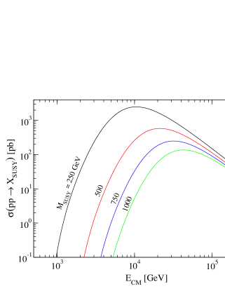
Figure 1: Total cross-section for $pp\to\,$SUSY as a function of $\sqrt{s}$ for several values of $M_{\rm SUSY}$.

Once a squark or gluino has been produced, it will decay in a cascade down to the the LSP. Presumably, one LSP of positive charge will be produced for each of negative charge. Searches for the latter are more difficult and we will concentrate only on the former. Further, we will assume conservatively that only one positively charged LSP is produced per SUSY interaction, though the number can be significantly higher as the cascades of decays progress. One expects that these positively charged LSPs form superheavy hydrogen by attracting a nearby electron and that this superheavy hydrogen eventually (over the lifetime of the earth) bonds into a superheavy water molecule in the earth’s oceans.

So as a final step we calculate the concentration of superheavy water in the oceans. Considering the age of the oceans, $t_{O}$, to be roughly 3 billions years, and assuming that the flux of cosmic rays has remained essentially unchanged over that time period, the number of superheavy water molecules per usual water molecule in the oceans (the “anomalous concentration”, $\chi$) is

$$\chi=7.6\times 10^{-13}\,\left(\frac{t_{O}}{3\,\mbox{Gyr}}\right)\left(\frac{2.6\,\mbox{km}}{d_{O}}\right)\times\frac{\Phi_{\rm SUSY}}{\mbox{cm}^{-2}\mbox{s}^{-1}\mbox{sr}^{-1}}$$

where $d_{O}$ is the average depth of the oceans.

The constraints on $\chi$ come from searches for superheavy molecules in large samples of water. Experiments then place bounds on $\chi$ as a function of the mass of the stable, charged particle. In our approach, this mass in unknown, though it is bounded from above by $M_{\rm SUSY}$. The strongest bound comes the experiment of Smith et al. [3], who find limits ranging from $\chi<3.5\times 10^{-30}$ for $m_{LSP}=100\,{\rm GeV}$ to $\chi<8\times 10^{-28}$ for $m_{LSP}=1.2\,{\rm TeV}$. Because their bound monotonically weakens as $m_{LSP}$ increases, we can place a very conservative bound on $M_{\rm SUSY}$ by setting $m_{LSP}=M_{\rm SUSY}$. For that case, we find $M_{\rm SUSY}>230\,{\rm GeV}$ if the LSP is stable and charged. (Our bound has an uncertainty of roughly $\pm 10\,{\rm GeV}$ due to a $\sim 50\%$ uncertainty that comes from the subtleties for defining $M_{\rm SUSY}$ discussed above.) These results are summarized in Figure 2 where we have shown the predicted anomalous concentration as a function of $M_{\rm SUSY}$ and the experimental bound of Ref. [3].

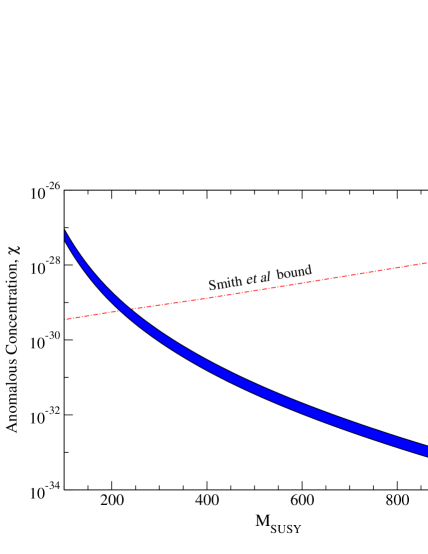
Figure 2: Anomalous concentration, $\chi$, of superheavy hydrogen in sea water as a function of the SUSY mass scale (shaded region). The bound of Ref. [3] is shown as a dashed line. The limits shown here assume $m_{LSP}=M_{\rm SUSY}$. The width of the shaded region represents a range of $\pm 50\%$ in the cross-section calculation due to model-dependence.

4 Conclusions

We have shown that there exist bounds from cosmic ray production in the upper atmosphere on charged stable relics (a charged SUSY LSP in particular) which are independent of cosmological constraints. Under the assumption that the incident cosmic ray flux has remained constant over the last 3 billion years, we have calculated a conservative lower bound on the scale of new physics ($M_{\rm SUSY}$), using nothing more than standard particle physics. If SUSY has a stable and charged LSP, then we can place a lower bound on the mass scale of the squarks and gluinos at 230 GeV.

This procedure can easily be extended to other models of weak-scale physics. In such a case, limits similar to those found here could be placed on the masses of new strongly-interacting particles.

Importantly, these bounds will not change if the basic paradigms of cosmology at and below the weak scale are questioned, such as happens in models with large extra dimensions. For example, it is unclear how standard cosmological bounds can be used to constrain models such as that of Ref. [7] which predicts a light, stable top squark but becomes non-perturbative and higher-dimensional at the TeV scale. The bound presented here should hold even in these highly non-standard cases.

Finally, if a charged particle is discovered which is stable on collider timescales, ruling out or verifying that it is stable on cosmological timescales will require that searches for superheavy water be examined again, though with larger initial samples. Unfortunately, the steeply falling cosmic ray spectrum requires us to go to exponentially larger samples in order to significantly increase our sensitivity. For example, the method used in Ref. [3] would require an initial heavy water sample equal to that contained in the SNO experiment in order to probe squark masses up to 700 GeV. While such a large-scale search seems unnecessary at present, any future discovery of a new stable, charged particle might require just such an effort. Otherwise there may be no other way to study the stability of that state on long timescales.

References

-
[1]
A. De Rujula, S. L. Glashow and U. Sarid,
Nucl. Phys. B 333, 173 (1990);
S. Dimopoulos, D. Eichler, R. Esmailzadeh and G. D. Starkman, Phys. Rev. D 41, 2388 (1990). -
[2]
P. F. Smith and J. R. Bennett,
Nucl. Phys. B 149, 525 (1979);
T. K. Hemmick et al., Phys. Rev. D 41, 2074 (1990);
P. Verkerk et al., Phys. Rev. Lett. 68, 1116 (1992);
T. Yamagata, Y. Takamori and H. Utsunomiya, Phys. Rev. D 47, 1231 (1993). - [3] P. F. Smith et al., Nucl. Phys. B 206, 333 (1982).
- [4] N. Arkani-Hamed, S. Dimopoulos, N. Kaloper and J. March-Russell, Nucl. Phys. B 567, 189 (2000).
-
[5]
D. J. Chung, E. W. Kolb and A. Riotto,
Phys. Rev. D 60, 063504 (1999);
G. F. Giudice, E. W. Kolb and A. Riotto, Phys. Rev. D 64, 023508 (2001). - [6] A. Kudo and M. Yamaguchi, Phys. Lett. B 516, 151 (2001).
- [7] R. Barbieri, L. J. Hall and Y. Nomura, Phys. Rev. D 63, 105007 (2001).
- [8] D. J. Bird et al. [HIRES Collaboration], Phys. Rev. Lett. 71, 3401 (1993).
- [9] Data from a variety of original experiments has been compiled in P. Greider, Cosmic Rays at Earth, Elsevier, Amsterdam (2001).
- [10] D. E. Groom et al. [Particle Data Group], Eur. Phys. J. C 15, 1 (2000).
- [11] W. Beenakker, R. Hopker, M. Spira and P. M. Zerwas, Nucl. Phys. B 492, 51 (1997).
- [12] H. L. Lai et al. [CTEQ Collaboration], Eur. Phys. J. C 12, 375 (2000).